Low-energy photon and pion scattering in holographic QCD

Abstract

Using holographic models where chiral symmetry is broken through IR b.c.’s, we determine a novel set of relations between QCD matrix elements. In particular, we find that the amplitudes of the three processes $\pi\pi\to\pi\pi$, $\gamma\gamma\to\pi\pi$ and $\gamma\to\pi\pi\pi$ involve a single scalar function $h(Q^{2})$ given by a suitable 5D integral of the EoM Green’s function. In a phenomenological analysis of $\gamma\gamma\to\pi\pi$ we find an overall agreement with the experimental cross section for a broad range of energy. Moreover, the polarizabilities at low energies show a fair agreement between the holographic approach, previous computations and experiment.

1 Introduction

Inspired by a holographic analysis of the axial-vector-vector ($AVV$) and left-right ($LR$) quark current Green’s functions Son:2010vc , several investigations have been devoted to the possible interplay between the anomalous and even intrinsic-parity sectors of Quantum Chromodynamics Colangelo:2011xk ; Iatrakis:2011ht ; Cappiello:2010tu ; Domokos:2011dn ; Alvares:2011wb ; Gorsky:2012ui ; Knecht:2011wh . In a recent study Colangelo:2012ip , using holographic models where chiral symmetry is realized nonlinearly through boundary conditions (b.c.’s) Son:2003et ; Sakai:2004cn ; Hirn:2005nr ; Sakai:2005yt , we derived a series of novel form factor and low-energy constant (LEC) relations in the limit of large number of colors $N_{C}\to\infty$ Nc . Here we continue along that line, and extend the analysis to scattering processes, going beyond the realm of static properties (mass spectra and couplings) and facing the more difficult dynamical problem of two-body scattering amplitudes. We focus on $\pi\pi$–scattering and on the radiative processes $\gamma\gamma\to\pi\pi$ and $\gamma\to 3\pi$, finding that it is possible to describe the three amplitudes through a single function determined by an appropriate 5D integral of the Green’s function of the five-dimensional equations of motion (EoM).

Chiral Perturbation theory ($\chi$PT) is the effective field theory describing the low-energy interaction of the pseudo-Goldstone bosons which emerge from the spontaneous breaking of the chiral symmetry Weinberg-chpt ; op4-chpt . The observables are obtained by a perturbative expansion in terms of the external momenta and the pseudoscalar mass, and involve a set of effective couplings Bijnens:1999hw ; Bijnens:1999sh ; Bijnens:2001bb ; Ebertshauser:2001nj . However, these couplings of the low-energy theory are not fixed by the symmetry, but need to be determined through other procedures. In Colangelo:2012ip we considered a set of holographic models without explicit chiral symmetry breaking, and computed all the LEC’s of the ${\cal O}(p^{6})$ $\chi$PT Lagrangian in the absence of scalar-pseudoscalar sources. As the LEC’s are independent of the quark masses, our results for the chiral couplings remain valid in the massive quark case.

Here, using the ${\cal O}(p^{6})$ LEC determinations in Colangelo:2012ip , we carry out a phenomenological analysis of the $\gamma\gamma\to\pi\pi$ reaction, as this matrix element depends on a transparent way on the ${\cal O}(p^{6})$ LEC’s Burgi:1996 ; Gasser:2005 ; Gasser:2006 . We also study the low-energy polarizabilities $(\alpha_{1}+\beta_{1})$ and $(\alpha_{2}\pm\beta_{2})$, defined below, whose lowest chiral orders are determined by the pion Born term and the ${\cal O}(p^{4})$ one-loop alone, with no contribution from ${\cal O}(p^{4})$ LEC’s Bijnens:1988 . The first tree-level contribution (in addition to the pion Born term) occurs at ${\cal O}(p^{6})$. Indeed, the polarizabilities $(\alpha_{1}+\beta_{1})$ and $(\alpha_{2}+\beta_{2})$ vanish at ${\cal O}(p^{2})$ and ${\cal O}(p^{4})$, starting the first non-vanishing contribution at ${\cal O}(p^{6})$. All this makes these observables an interesting benchmark for the ${\cal O}(p^{6})$ LEC determination in Colangelo:2012ip . We find that the relevant combinations of chiral couplings are fully determined by the anomalous Chern-Simons action and are universal for this kind of holographic models, since they are independent of the details of the 5D background Colangelo:2012ip . In addition, we observe that the experimental $\gamma\gamma\to\pi\pi$ cross section is reproduced even in the region away from the threshold.

The article is organized as follows. In Sec. 2 we recall the holographic setup used to calculate the LEC and their relations. In Sec. 3 we show that a unique function appears in several $\pi\pi$ and $\gamma\gamma$ scattering amplitudes, so that relations can be worked out among these amplitudes and they can be experimentally tested. In Sec. 4 we study the polarizabilities in $\gamma\gamma\to\pi\pi$ scattering, and compare the results obtained in our holographic approach to a few experimental and theoretical determinations. Then, we draw our conclusions.

2 Holographic setup

We restrict ourselves to a class of holographic models where chiral symmetry is realized nonlinearly, through suitable boundary conditions. This class of models was proposed in ref. Son:2003et , developed in refs. Sakai:2004cn ; Hirn:2005nr ; Sakai:2005yt , and further studied in refs. Son:2010vc ; Colangelo:2012ip . The gauge group is $U(n_{f})$, and the $5D$ action is composed by the Yang–Mills (YM) and Chern–Simons (CS) terms, describing the intrinsic even-parity and the anomalous QCD sectors, respectively Son:2003et ; Hirn:2005nr ; Sakai:2004cn ; Sakai:2005yt :

$$S=S_{\rm YM}+S_{\rm CS}$$ (1)

with

$$S_{\rm YM} = -\int\,\,d^{5}x\,\,{\rm Tr}\left[-f^{2}(z){\cal F}_{z\mu}^{2}+\frac{1}{2g^{2}(z)}{\cal F}_{\mu\nu}^{2}\right],$$ (2)

$$S_{\rm CS} = -\kappa\int\,\,{\rm Tr}\left[{\cal AF}^{2}+\frac{i}{2}{\cal A}^{3}{\cal F}-\frac{1}{10}{\cal A}^{5}\right].$$ (3)

The fifth coordinate $z$ runs from $-z_{0}$ to $z_{0}$, with $0<z_{0}\leq+\infty$. ${\cal A}(x,z)={\cal A}_{M}dx^{M}$ is the 5D gauge field and ${\cal F}=d{\cal A}-i{\cal A}\wedge{\cal A}$ the field strength. In terms of the $U(n_{f})$ generators $t^{a}$, normalized as $Tr[t^{a}t^{b}]=\delta^{ab}/2$, they read: ${\cal A}={\cal A}^{a}t^{a}$ and ${\cal F}={\cal F}^{a}t^{a}$. The coefficient $\kappa=N_{C}/(24\pi^{2})$ is fixed by the chiral anomaly of QCD Wess:1971yu ; Witten:1983tw .

If the functions $f^{2}(z)$ and $g^{2}(z)$ in (2) are invariant under reflection $z\to-z$, parity can be properly defined in these models. In appendix A other conditions necessary to derive physical LEC’s are discussed. Moreover, in appendix B we provide the profiles of $f(z)$ and $g(z)$ for the flat metric Son:2003et , “Cosh” Son:2003et , Hard-Wall Hirn:2005nr and Sakai-Sugimoto models Sakai:2004cn ; Sakai:2005yt that are used below. In all these models a common coupling constant $g_{5}^{-2}$ appears in $f^{2}(z)$ and $g^{-2}(z)$. In asymptotically anti-de Sitter backgrounds this coupling can be fixed to be $g_{5}^{-2}=N_{C}/(24\pi^{2})$ Son:2003et through the high-energy behaviour of the two-point correlation function of quark vector currents. For general backgrounds, both $f^{2}(z)$ and $g^{-2}(z)$ should always contain a factor of $N_{C}$, in order to match the $N_{C}$-dependence of the LEC’s. For example, one has

$$F^{2} = 4\left(\int_{-z_{0}}^{z_{0}}\frac{\mathrm{d}z}{f^{2}(z)}\right)^{-1}\,,$$

$$L_{1} = \frac{1}{2}L_{2}=-\frac{1}{6}L_{3}=\frac{1}{32}\int_{-z_{0}}^{z_{0}}\frac{(1-\psi_{0}^{2})^{2}}{g^{2}(z)}\,\mathrm{d}z\,,$$ (4)

and all of them are ${\cal O}(N_{C})$, as expected.

As discussed in details in ref. Colangelo:2012ip , in (1) the QCD chiral symmetry is promoted to a 5D gauge symmetry, with the possibility of naturally introducing the right- and left-handed current sources, $r_{\mu}(x)$ and $\ell_{\mu}(x)$ respectively. The Goldstone bosons are contained in the ${\cal A}_{z}$ component of the gauge field, and are described through the chiral field $U$, given by the Wilson line

$$U(x^{\mu})=\mbox{P}\exp\left\{i\int^{+z_{0}}_{-z_{0}}{\cal A}_{z}(x^{\mu},z^{\prime})dz^{\prime}\right\}.$$ (5)

This field transforms as

$$U(x)\to g_{R}(x)U(x)g_{L}^{\dagger}(x)$$ (6)

with $g_{L}(x)$ and $g_{R}(x)$ the left and right gauge transformations localized at $z=-z_{0}$ and $z=z_{0}$, respectively. The ${\cal A}_{\mu}$ components of the gauge fields contain vector and axial-vector resonances, since

$${\cal A}_{\mu}(x,z)=\ell_{\mu}(x)\psi_{-}(z)+r_{\mu}(x)\psi_{+}(z)+\sum_{n=1}^{\infty}B_{\mu}^{(n)}(x)\psi_{n}(z)\,.$$ (7)

The ultraviolet (UV) boundary conditions

$$\mathcal{A}_{\mu}(x,-z_{0})=\ell_{\mu}(x)\,,\qquad\qquad\mathcal{A}_{\mu}(x,z_{0})=r_{\mu}(x)\,$$ (8)

are imposed. In Eq.(7) the functions $\psi_{\pm}(z)=\frac{1}{2}(1\pm\psi_{0}(z))$ are determined by the $\psi_{0}(z)$ solution of the 5D EoM of the ${\cal A}_{\mu}(x,z)$ gauge fields corresponding to the zero mode, with b.c.’s $\psi_{0}(\pm z_{0})=\pm 1$. On the other hand, the $\psi_{n}(z)$ correspond to the resonant modes with mass $m_{n}$; their b.c.’s are $\psi_{n}(\pm z_{0})=0$. Under a suitable gauge transformation it is possible to set $\mathcal{A}_{z}=0$, with the space-time components of the 5D field taking the form

$${\cal A}_{\mu}(x,z)=i\Gamma_{\mu}(x)+\frac{u_{\mu}(x)}{2}\psi_{0}(z)+\sum_{n=1}^{\infty}v_{\mu}^{n}(x)\psi_{2n-1}(z)+\sum_{n=1}^{\infty}a_{\mu}^{n}(x)\psi_{2n}(z)\,,$$ (9)

where the tensors $u_{\mu}(x)$ and $\Gamma_{\mu}(x)$, commonly used in $\chi$PT Bijnens:1999sh ; Bijnens:1999hw ; RChTa+b ; RChTc , naturally show up:

$$u_{\mu}\left(x\right) \equiv \mathrm{i}\left\{\xi_{R}^{{\dagger}}\left(x\right)\left(\partial_{\mu}-\mathrm{i}r_{\mu}\right)\xi_{R}\left(x\right)-\xi_{L}^{{\dagger}}\left(x\right)\left(\partial_{\mu}-\mathrm{i}\ell_{\mu}\right)\xi_{L}\left(x\right)\right\}$$ (10)

$$\Gamma_{\mu}\left(x\right) \equiv \frac{1}{2}\left\{\xi_{R}^{{\dagger}}\left(x\right)\left(\partial_{\mu}-\mathrm{i}r_{\mu}\right)\xi_{R}\left(x\right)+\xi^{{\dagger}}_{L}\left(x\right)\left(\partial_{\mu}-\mathrm{i}\ell_{\mu}\right)\xi_{L}\left(x\right)\right\},$$ (11)

with the non-linear realization $u(x)=\xi_{R}(x)=\xi_{L}^{\dagger}(x)=\exp\{i\pi^{a}t^{a}/F\}$.

The 5D action can be expressed using the decomposition (9) of the 5D gauge fields in resonances and the non-linearly realized chiral Goldstone bosons Sakai:2004cn ; Hirn:2005nr ; Sakai:2005yt ; Colangelo:2012ip . The resulting 4D action terms relevant for our analysis contain operators with only Goldstones (see appendix A) and pieces with one resonance field $v^{n}_{\mu}$, together with the couplings $b_{v^{n}\pi\pi}$, $c_{v^{n}}$ and $d_{v^{n}}$:

$$S_{\rm{YM}}\Big{|}_{1-res} = -\,\sum_{n}\frac{i\,b_{v^{n}\pi\pi}}{4}\,\int\mathrm{d}^{4}x\langle\,(\nabla_{\mu}v_{\nu}^{n}-\nabla_{\nu}v_{\mu}^{n})[u^{\mu},u^{\nu}]\,\rangle\,\,\,+\,\,\,...$$ (12)

$$S_{\rm{CS}}\Big{|}_{1-res} = \,\sum_{n}\,\epsilon^{\mu\nu\alpha\beta}\,\int\mathrm{d}^{4}x\,\bigg{[}-\frac{N_{C}}{32\pi^{2}}c_{v^{n}}\langle\,u_{\mu}\{v_{\nu}^{n},f_{+\alpha\beta}\}\,\rangle+\frac{iN_{C}}{16\pi^{2}}\,(c_{v^{n}}-d_{v^{n}})\langle\,v_{\mu}^{n}u_{\nu}u_{\alpha}u_{\beta}\,\rangle\,\bigg{]}$$ (13)

$$+\,\,\,...$$

with $v_{\mu}^{n}=v_{\mu}^{n,\,a}\,t^{a}$ and the covariant tensor $f_{+}^{\alpha\beta}=\xi_{R}^{\dagger}F_{R}^{\alpha\beta}\xi_{R}+\xi_{L}^{\dagger}F_{L}^{\alpha\beta}\xi_{L}$ provided by the left and right source field-strength tensors Bijnens:1999sh ; Bijnens:1999hw ; RChTa+b ; RChTc . The couplings are given by the integrals of the corresponding 5D wave functions:

$$b_{v^{n}\pi\pi} = \int_{-z_{0}}^{z_{0}}\frac{\psi_{2n-1}(z)\,(1-\psi_{0}(z)^{2})}{g^{2}(z)}\,\mathrm{d}z\,,$$

$$c_{v^{n}} = -\frac{1}{2}\int_{-z_{0}}^{z_{0}}\psi_{0}(z)\,\psi_{2n-1}^{\prime}(z)\mathrm{d}z\,,$$ (14)

$$d_{v^{n}} = \frac{1}{2}\int_{-z_{0}}^{z_{0}}\psi_{0}(z)^{2}\,\psi_{0}^{\prime}(z)\,\psi_{2n-1}(z)\,\mathrm{d}z\,.$$

The primes denote derivative with respect to $z$. Using the EoM of $\psi_{n}(z)$ the relation

$$c_{v^{n}} = g_{v^{n}\pi\pi}\,\,\,$$ (15)

is obtained Sakai:2005yt ; Colangelo:2012ip , with $\displaystyle g_{v^{n}\pi\pi}=\frac{m_{v^{n}}^{2}}{2F^{2}}b_{v^{n}\pi\pi}$ the coupling between the vector resonance $v^{n}$ and a pion pair. This equation implies a connection between the $v^{n}\to\pi\pi$ and $v^{n}\to\pi\gamma$ decay widths which are determined by the couplings $g_{v^{n}\pi\pi}$ and $c_{v^{n}}$, respectively, and represents the key ingredient for the relations between amplitudes exploited in the following. Another important property in the considered models is that the vertex $a^{n}\pi\gamma$ vanishes Hirn:2005nr ; Colangelo:2012ip , therefore all the amplitudes studied below do not get contributions from the axial-vector resonances.

One may wonder whether the relation (15) is experimentally fulfilled. The experimental results for the lightest vector mesons are Sakai:2005yt

$$c_{\omega}|_{\rm exp}\,\,\,=\,\,\,5.80\,\,\,,\qquad\qquad g_{\rho\pi\pi}|_{\rm exp}\,\,\,=\,\,\,5.99\,\,\,\,,$$ (16)

determined from the measured $\omega\to\pi^{0}\gamma$ and $\rho\to\pi\pi$ decay rates, respectively Beringer:1900zz . On the other hand, in the holographic analysis in ref. Colangelo:2012ip we found for the considered 5D models the results in Table 1, all close to the experimental data. In each case and all along the paper, the mass of the lightest vector meson $m_{\rho}=776$ MeV and the pion decay constant $F=87$ MeV are taken as inputs to set the parameters of the 5D model Colangelo:2012ip . Since the action (1) does not incorporate quark masses, all the interaction vertices are predicted in the chiral limit. This allows us to extract some relevant combinations of LEC’s, as they are quark mass independent. However, in the computation of cross sections and decay widths we consider the physical pion mass in the phase-space factors, assuming that this captures the most important quark mass corrections. Likewise, no scalar states or resonances with spin $S\geq 2$ are included in the present analysis.

	Flat	Cosh	Hard-Wall	Sakai-Sugimoto
$g_{\rho\pi\pi}=c_{\rho}$	5.11	5.14	5.13	5.11

Table 1: Couplings $g_{\rho\pi\pi}$ and $c_{\rho}$ determined in four holographic QCD models.

3 Holographic description of scattering amplitudes

3.1 $\pi\pi$ scattering

We consider the $\pi\pi$ scattering in the holographic framework. The scattering amplitude can be easily derived with the 4D resonance Lagrangian (12), together with the ${\cal O}(p^{4})$ chiral Lagrangian resulting from the YM action (2). As we shall see below, the summation over the resonances can be transformed into a single function $h(Q^{2})$ given by an integral involving the 5D Green’s function.

The $\pi^{a}\pi^{b}\to\pi^{c}\pi^{d}$ scattering amplitude is provided by the isospin decomposition

$$A(\pi^{a}\pi^{b}\to\pi^{c}\pi^{d}) = A(s,t,u)\delta^{ab}\delta^{cd}\,+\,A(t,s,u)\delta^{ac}\delta^{bd}\,+\,A(u,t,s)\delta^{ad}\delta^{bc}\,,$$ (17)

with $s=(p_{a}+p_{b})^{2}$, $t=(p_{a}-p_{c})^{2}$, $u=(p_{a}-p_{d})^{2}$ and the Mandelstam relation $s+t+u=0$ in the massless pion limit. The holographic action yields the $v^{n}\pi\pi$ Lagrangian (12), in addition to direct $\pi\pi\to\pi\pi$ vertices, giving the amplitude

$$A(s,t,u) = \frac{\displaystyle s}{\displaystyle F^{2}}+\frac{\displaystyle 4L_{1}((t-u)^{2}-3s^{2})}{\displaystyle F^{4}}+\sum_{n}\frac{\displaystyle b_{v^{n}\pi\pi}^{2}}{\displaystyle 4F^{4}}\bigg{[}\frac{\displaystyle t^{2}(t+2s)}{\displaystyle m_{v^{n}}^{2}-t}+\frac{\displaystyle u^{2}(u+2s)}{\displaystyle m_{v^{n}}^{2}-u}\bigg{]}$$ (18)

$$= \sum_{n}g_{v^{n}\pi\pi}^{2}\bigg{[}\frac{\displaystyle t+2s}{\displaystyle m_{v^{n}}^{2}-t}+\frac{\displaystyle u+2s}{\displaystyle m_{v^{n}}^{2}-u}\bigg{]}\,$$

obtained using the definition of $g_{v^{n}\pi\pi}$ together with the sum rules Colangelo:2012ip ; Hirn:2005nr

$$\sum_{n}b_{v^{n}\pi\pi}^{2}=32L_{1}\,\,\,\,,\,\,\,\,\,\sum_{n}b_{v^{n}\pi\pi}^{2}m_{v^{n}}^{2}=\frac{4F^{2}}{3}\,.$$ (19)

It is possible to express the $\pi\pi$–scattering amplitude (18) in a holographic form,

$$A(s,t,u) = \frac{\displaystyle 1}{\displaystyle 4}\displaystyle{\int}_{-z_{0}}^{z_{0}}dz\,\,\displaystyle{\int}_{-z_{0}}^{z_{0}}dz^{\prime}\,\,\psi_{0}^{\prime}(z)\psi_{0}^{\prime}(z^{\prime})\,\bigg{[}(t+2s)\,G(-t;z,z^{\prime})\,+\,(u+2s)\,G(-u;z,z^{\prime})\bigg{]}$$ (20)

$$= \frac{\displaystyle 1}{\displaystyle 4}\,\,\bigg{[}(t+2s)\,h(-t)\,+\,(u+2s)\,h(-u)\bigg{]}\,,$$

in terms of the function $h(Q^{2})$ obtained from the integral of the Green’s function $G(Q^{2};z,z^{\prime})$ in the $z$ (holographic) coordinate:

$$h(Q^{2}) = \displaystyle{\int}_{-z_{0}}^{z_{0}}dz\,\,\displaystyle{\int}_{-z_{0}}^{z_{0}}dz^{\prime}\,\psi_{0}^{\prime}(z)\psi_{0}^{\prime}(z^{\prime})\,G(Q^{2};z,z^{\prime})\,,$$ (21)

$$G(Q^{2};z,z^{\prime}) = \sum_{n=1}^{\infty}\frac{\displaystyle\psi_{n}(z)\psi_{n}(z^{\prime})}{\displaystyle m_{n}^{2}+Q^{2}}\,.$$ (22)

To rewrite (18) into (20) we made use of the relation in Eq. (15). It is useful to express the $h(Q^{2})$ function in terms of resonance exchanges,

$$h(Q^{2}) = \sum_{n}\frac{\displaystyle 4g_{v^{n}\pi\pi}^{2}}{\displaystyle m_{v^{n}}^{2}+Q^{2}}\,\,\,=\,\,\,\sum_{n}\frac{\displaystyle 4c_{v^{n}}^{2}}{\displaystyle m_{v^{n}}^{2}+Q^{2}}\,.$$ (23)

With the help of the sum-rules (19) the low-energy expansion can be worked out:

$$h(Q^{2}) = \frac{\displaystyle 4}{\displaystyle 3F^{2}}\,-\,\frac{\displaystyle 32L_{1}Q^{2}}{\displaystyle F^{4}}\,+\,\frac{\displaystyle 32(C_{1}+4C_{3})Q^{4}}{\displaystyle F^{4}}\,+\,{\cal O}(Q^{6})\,.$$ (24)

We also used the ${\cal O}(p^{6})$ relations $(C_{1}+4C_{3})=(3C_{3}+C_{4})=\sum_{n}F^{4}g_{v^{n}\pi\pi}^{2}/(8m_{v^{n}}^{6})$ derived in Colangelo:2012ip . The right low-energy expansion of the $\pi\pi$–scattering amplitude at large $N_{C}$ op4-chpt ; op6-pipi-scat is recovered,

$$A(s,t,u)^{\rm\chi PT} = \frac{\displaystyle s}{\displaystyle F^{2}}\,+\,\frac{\displaystyle 8L_{1}\,(t^{2}+u^{2}-2s^{2})}{\displaystyle F^{4}}\,-\,\frac{\displaystyle 8(C_{1}+4C_{3})(t+u)(t^{2}+tu+u^{2})}{\displaystyle F^{4}}\,\,\,+\,\,\,{\cal O}(p^{8})\,.$$

Notice that, in the large-$N_{C}$ limit, in the absence of other resonances, $L_{2}$ and $L_{3}$ are both related to the low-energy constant $L_{1}$ RChTa+b : $\displaystyle{L_{2}}/{2}=-{L_{3}}/{6}=L_{1}$. In a similar way, at large–$N_{C}$ one has $C_{2}=0$ and $(C_{1}+4C_{3})=(3C_{3}+C_{4})$ when just vector resonance exchanges are taken into account RChTc ; Guo:2007 . This result provides a consistency check of the holographic derivation and of the determination in Colangelo:2012ip of the ${\cal O}(p^{6})$ low energy constants.

The large-$Q^{2}$ behavior of the function $h(Q^{2})$ also determines the high energy behavior of the scattering amplitudes. This can be obtained from the resonance expression (23), and depends on the convergence of the sum

$$\mathcal{H}\equiv\sum_{n=0}^{\infty}~{}c_{v^{n}}^{2}\,\,\,.$$ (26)

As long as this sum converges, one has

$$h(Q^{2})\quad\stackrel{{\scriptstyle Q^{2}\to\infty}}{{\longrightarrow}}\quad\frac{4\mathcal{H}}{Q^{2}}\,\,\,.$$ (27)

Using the holographic expression for $c_{v^{n}}$, we can rewrite the sum as a 5D integral,

$$\mathcal{H}=\frac{1}{4}\int_{-z_{0}}^{z_{0}}~{}[\psi^{\prime}_{0}(z)]^{2}~{}g^{2}(z)\mathrm{d}z=\frac{F^{4}}{16}\int_{-z_{0}}^{z_{0}}~{}\frac{g^{2}(z)}{f^{4}(z)}\mathrm{d}z\,\,\,.$$ (28)

For arbitrary background functions $f^{2}(z)$ and $g^{2}(z)$ this integral may diverge. However, if we restrict ourselves to the case when the kinetic coefficient $H_{1}$ of the external sources in the ${\cal O}(p^{4})$ $\chi$PT Lagrangian is UV–divergent , we can prove in general that $\mathcal{H}$ is finite, as shown in appendix A. This is true for all the models listed in appendix B, although the explicit values of the resonance parameters and of the sum are different in each case. For example, one has $\mathcal{H}=g_{5}^{2}/2=4m_{\rho}^{2}/(\pi^{2}F^{2})$ and $\mathcal{H}=g_{5}^{2}/3=m_{\rho}^{2}/(3F^{2})$ for the Flat and “Cosh” models, respectively. It is interesting to remark that, contrary to other matrix elements such as the two-point vector current correlation function, the short-distance power behavior is similar for models with very different backgrounds near the UV boundary. The reason may be that only when we take the momentum square of the external source to be large, as we usually do in the vector correlator and in form factors involving pions, we probe the ultraviolet region of the backgrounds. For instance, in the isospin $I=2$ channel one has $T^{2}(s,t,u)=A(t,s,u)+A(u,t,s)$, and the large-$s$ behaviour of the corresponding $J=0$ partial wave is

$$T^{2}_{0}(s)=-\,\frac{\displaystyle 1}{\displaystyle 64\pi s}\displaystyle{\int}_{-s}^{0}\,(t+2s)\,h(-t)\,d{\rm t}\quad\stackrel{{\scriptstyle s\to\infty}}{{\longrightarrow}}\quad-\frac{\mathcal{H}}{8\pi}\ln\frac{s}{\Lambda^{2}}+{\cal O}(s^{0})\,.$$ (29)

The parameter $\Lambda$ is a finite hadronic scale arising from the integration. Thus, the residual logarithmic behavior found at high energies in the case of a finite number of vector exchanges Guo:2007 ; Nieves:2011 shows up also in holographic models, with an infinite tower of resonances. Calculations of higher partial waves give a similar logarithmic behavior.

3.2 $\gamma\gamma\to\pi\pi$ scattering

We now analyze an observable for which the odd intrinsic-parity sector of the action plays a crucial role, the radiative process $\gamma\gamma\to\pi\pi$. We first perform a separate theoretical study of the neutral and charged modes. Nonetheless, our holographic description provides pretty similar structures for both of them.

3.2.1 $\gamma\gamma\to\pi^{0}\pi^{0}$

The $\gamma(k_{1},\epsilon_{1})\gamma(k_{2},\epsilon_{2})\to\pi^{0}(p_{1})\pi^{0}(p_{2})$ scattering amplitude is described by two structure functions, $A(s,t,u)^{\gamma\gamma\to\pi^{0}\pi^{0}}$ and $B(s,t,u)^{\gamma\gamma\to\pi^{0}\pi^{0}}$:

$$T^{\gamma\gamma\to\pi^{0}\pi^{0}} = e^{2}(\epsilon_{1}^{\mu}\epsilon_{2}^{\nu}T^{(1)}_{\mu\nu})\times A(s,t,u)^{\gamma\gamma\to\pi^{0}\pi^{0}}\,\,\,+\,\,\,e^{2}(\epsilon_{1}^{\mu}\epsilon_{2}^{\nu}T^{(2)}_{\mu\nu})\times B(s,t,u)^{\gamma\gamma\to\pi^{0}\pi^{0}}\,.$$

The Lorentz structures are defined as $(\epsilon_{1}^{\mu}\epsilon_{2}^{\nu}T^{(1)}_{\mu\nu})=\frac{s}{2}(\epsilon_{1}\epsilon_{2})-(\epsilon_{1}k_{2})(\epsilon_{2}k_{1})$ and $(\epsilon_{1}^{\mu}\epsilon_{2}^{\nu}T^{(2)}_{\mu\nu})=2s(\epsilon_{1}\Delta)(\epsilon_{2}\Delta)-(t-u)^{2}(\epsilon_{1}\epsilon_{2})-2(t-u)[(\epsilon_{1}\Delta)(\epsilon_{2}k_{1})-(\epsilon_{1}k_{2})(\epsilon_{2}\Delta)]$, with $\Delta^{\mu}\equiv p_{1}^{\mu}-p_{2}^{\mu}$ and $\epsilon_{i}$ the photon polarization vectors.

In $\chi$PT, the neutral $\pi\pi$ channel has no contribution at ${\cal O}(p^{2})$, and at ${\cal O}(p^{4})$ there is no tree-level, but only one-loop diagrams. Thus, at large-$N_{C}$ the contributions to the $\gamma\gamma\to\pi^{0}\pi^{0}$ amplitude start at ${\cal O}(p^{6})$ and read Burgi:1996 ; Gasser:2005

$$A(s,t,u)^{\gamma\gamma\to\pi^{0}\pi^{0}} = \frac{\displaystyle 1}{\displaystyle(4\pi F)^{4}}\,(a_{1}m_{\pi}^{2}+a_{2}s)\,\,\,+\,\,\,{\cal O}(E^{4})\,,$$

$$B(s,t,u)^{\gamma\gamma\to\pi^{0}\pi^{0}} = \frac{\displaystyle b}{\displaystyle(4\pi F)^{4}}\,\,\,+\,\,\,{\cal O}(E^{2})\,,$$ (31)

with $s,t,u,m_{\pi}^{2}={\cal O}(E^{2})$. Since our holographic approach does not incorporate quark masses, the term with $a_{1}$ is out of the reach of the present work, and we focus on observables that do not contain it. In (31) the parameters $a_{2}$ and $b$ are combinations of LEC’s. For three flavors and symmetry group $SU(3)$, the electric charge matrix is Q=diag$(2/3,-1/3,-1/3)$, and one finds the large–$N_{C}$ low-energy parameters

$$a_{2} = \frac{\displaystyle 10}{\displaystyle 9}\times 256\pi^{4}F^{2}\bigg{(}8C_{53}+8C_{55}+C_{56}+C_{57}+2C_{59}\bigg{)}\,$$

$$b = -\,\frac{\displaystyle 10}{\displaystyle 9}\times 128\pi^{4}F^{2}\bigg{(}C_{56}+C_{57}+2C_{59}\bigg{)}\,.$$ (32)

In the holographic calculation Colangelo:2012ip we obtained predictions for the ${\cal O}(p^{6})$ LEC’s, which yield particularly simple expressions,

$$a_{2} = \frac{\displaystyle 10}{\displaystyle 9}\times 3N_{C}^{2}F^{2}\sum_{n}\frac{\displaystyle c_{v^{n}}^{2}}{\displaystyle m_{v^{n}}^{2}}\,\,\,=\,\,\,\frac{\displaystyle 10}{\displaystyle 9}\times N_{C}^{2}\,$$

$$b = \frac{\displaystyle 10}{\displaystyle 9}\times\frac{\displaystyle N_{C}^{2}F^{2}}{\displaystyle 2}\sum_{n}\frac{\displaystyle c_{v^{n}}^{2}}{\displaystyle m_{v^{n}}^{2}}\,\,\,=\,\,\,\frac{\displaystyle 10}{\displaystyle 9}\times\frac{\displaystyle N_{C}^{2}}{\displaystyle 6}\,$$ (33)

using the sum rule $\sum_{n}c_{v^{n}}^{2}/m_{v^{n}}^{2}=\sum_{n}g_{v^{n}\pi\pi}^{2}/m_{v^{n}}^{2}=1/(3F^{2})$ derived in Colangelo:2012ip . The expressions for the relevant LEC’s are collected in appendix D.

At higher energy it is possible to express our holographic result for the massless quark case in terms of the same function $h(Q^{2})$:

$$A(s,t,u)^{\gamma\gamma\to\pi^{0}\pi^{0}} = \frac{\displaystyle a_{2}}{\displaystyle(4\pi F)^{4}}\bigg{[}\frac{\displaystyle(s-4t)}{\displaystyle 2}\,\sum_{n}\frac{\displaystyle F^{2}c_{v^{n}}^{2}}{\displaystyle m_{v^{n}}^{2}-t}\,\,\,+\,\,\,(t\leftrightarrow u)\bigg{]}$$ (34)

$$= \frac{\displaystyle a_{2}}{\displaystyle(4\pi F)^{4}}\bigg{[}\frac{\displaystyle(s-4t)}{\displaystyle 8}\,F^{2}h(-t)\,\,\,+\,\,\,(t\leftrightarrow u)\bigg{]}$$

$$= \frac{\displaystyle a_{2}}{\displaystyle(4\pi F)^{4}}\bigg{[}s\,\,+\,\,\frac{\displaystyle 4L_{1}}{\displaystyle F^{2}}(8tu-5s^{2})\,\,+\,\,{\cal O}(E^{6})\bigg{]}\,,$$

$$B(s,t,u)^{\gamma\gamma\to\pi^{0}\pi^{0}} = \frac{\displaystyle b}{\displaystyle(4\pi F)^{4}}\bigg{[}\frac{\displaystyle 3}{\displaystyle 2}\,\sum_{n}\frac{\displaystyle F^{2}c_{v^{n}}^{2}}{\displaystyle m_{v^{n}}^{2}-t}\,\,\,+\,\,\,(t\leftrightarrow u)\bigg{]}$$ (35)

$$= \frac{\displaystyle b}{\displaystyle(4\pi F)^{4}}\bigg{[}\frac{\displaystyle 3}{\displaystyle 8}\,F^{2}h(-t)\,\,\,+\,\,\,(t\leftrightarrow u)\bigg{]}$$

$$= \frac{\displaystyle b}{\displaystyle(4\pi F)^{4}}\bigg{[}1\,\,-\,\,\frac{\displaystyle 12L_{1}s}{\displaystyle F^{2}}\,\,+\,\,{\cal O}(E^{4})\bigg{]}\,,$$

with $a_{2}$ and $b$ given in Eq. (33) and the low-energy expansion of $h(Q^{2})$ in (24). We have kept the chiral expansion up to ${\cal O}(p^{8})$, as later we will analyze the polarizability $(\alpha_{2}+\beta_{2})$ which starts at that order at large–$N_{C}$.

For $N_{C}\to\infty$ the strange quark does not play a role in this amplitude and our holographic description yields the same prediction in $U(2)$ and $U(3)$. Moreover, since in the external legs we only have pions and non-singlet components in the electromagnetic gauge field ($J_{\mu}^{\rm em}=J_{\mu}^{3}+\frac{1}{\sqrt{3}}J_{\mu}^{8}$), the $U(3)$ result is identical to the $SU(3)$ one. It is clarifying to observe the $\gamma\to\pi V$ vertex obtained from the Lagrangian (13) in the $SU(3)$ case,

$$\mathcal{L} = \sum_{n}\frac{\displaystyle eN_{C}c_{v^{n}}}{\displaystyle 8\pi^{2}F}\,\epsilon^{\rho\sigma\mu\nu}\partial_{\rho}V_{\sigma}^{\rm em}\,\bigg{[}\frac{\displaystyle 1}{\displaystyle 3}\bigg{(}\partial_{\mu}\pi^{0}\,\rho^{0,n}_{\nu}+\partial_{\mu}\pi^{+}\,\rho^{-,n}_{\nu}+\partial_{\mu}\pi^{-}\,\rho^{+,n}_{\nu}\bigg{)}+\partial_{\mu}\pi^{0}\,\omega^{n}_{\nu}\bigg{]}\,\,\,+\,\,\,...$$

coincides with the one found in previous approaches based on resonance Lagrangians Ko:1990 ; Babusci:1993 .

If we restrict ourselves to $SU(2)$ with Q=diag$(1/2,-1/2)$ (but allowing the $SU(2)$ singlet resonance $\omega$), all the $\rho^{\pm,0}$ terms vanish and only the $\omega$ resonance exchange survives. Thus, the ${\cal O}(p^{6})$ $\chi$PT contribution at large $N_{C}$ Gasser:2005 ,

$$a_{2} = 256\pi^{4}F^{2}\bigg{(}8C_{53}+8C_{55}+C_{56}+C_{57}+2C_{59}\bigg{)}\,,$$

$$b = -\,128\pi^{4}F^{2}\bigg{(}C_{56}+C_{57}+2C_{59}\bigg{)}\,,$$ (37)

becomes Colangelo:2012ip

$$a_{2}=N_{C}^{2}\,\,\,\,,\qquad\qquad b=\frac{\displaystyle N_{C}^{2}}{\displaystyle 6}\,\,\,\,.$$ (38)

Notice that we have used the $SU(3)$ notation for the corresponding $SU(2)$ couplings at large $N_{C}$. In $SU(2)$ notation one would have to make the replacement $C_{53}\to c_{29}$, $C_{55}\to c_{30}$, $C_{56}\to c_{31}$, $C_{57}\to c_{32}$ and $C_{59}\to c_{33}$ Bijnens:2001bb . In the following phenomenological analysis we always consider the large–$N_{C}$ estimates with the charge matrix Q=diag$(2/3,-1/3,-1/3)$.

3.2.2 $\gamma\gamma\to\pi^{+}\pi^{-}$

The charged pion mode contains the Born term at ${\cal O}(p^{2})$ in the chiral expansion, given by the pion exchange diagram. At ${\cal O}(p^{4})$ there is a tree-level contribution proportional to $(L_{9}+L_{10})$ and one-loop diagrams. Hence, at large-$N_{C}$ (where loop diagrams provide a subleading contribution) we have the chiral expansion Burgi:1996 ; Bijnens:1988 ; Gasser:2005 ; Gasser:2006 :

$$A(s,t,u)^{\gamma\gamma\to\pi^{+}\pi^{-}} = \frac{\displaystyle 1}{\displaystyle m_{\pi}^{2}-t}+\frac{\displaystyle 1}{\displaystyle m_{\pi}^{2}-u}\,\,\,+\,\,\,\frac{\displaystyle 8(L_{9}+L_{10})}{\displaystyle F^{2}}\,\,\,+\,\,\,\frac{\displaystyle(a_{1}m_{\pi}^{2}+a_{2}s)}{\displaystyle(4\pi F)^{4}}\,\,\,+\,\,\,{\cal O}(E^{4})\,,$$

$$B(s,t,u)^{\gamma\gamma\to\pi^{+}\pi^{-}} = \frac{\displaystyle 1}{\displaystyle 2s}\bigg{[}\frac{\displaystyle 1}{\displaystyle m_{\pi}^{2}-t}+\frac{\displaystyle 1}{\displaystyle m_{\pi}^{2}-u}\bigg{]}\,\,\,+\,\,\,\frac{\displaystyle b}{\displaystyle(4\pi F)^{4}}\,\,\,+\,\,\,{\cal O}(E^{2})\,,$$ (39)

with $s,t,u,m_{\pi}^{2}={\cal O}(E^{2})$. In the three-flavor $SU(3)$ case, $a_{2}$ and $b$ are given by the combinations of ${\cal O}(p^{6})$ LEC’s,

$$a_{2} = \frac{\displaystyle 10}{\displaystyle 9}\times 256\pi^{4}F^{2}\bigg{(}8C_{53}-\frac{4}{5}\times 8C_{55}+C_{56}+C_{57}-\frac{4}{5}\times 2C_{59}$$

$$\qquad\qquad\qquad\qquad+\frac{9}{10}\times 4C_{78}+\frac{9}{10}\times 8C_{87}-\frac{9}{10}\times 4C_{88}\bigg{)}\,,$$

$$b = -\,\frac{\displaystyle 10}{\displaystyle 9}\times 128\pi^{4}F^{2}\bigg{(}C_{56}+C_{57}-\frac{4}{5}\times 2C_{59}-\frac{9}{10}\times 4C_{78}\bigg{)}\,.$$ (40)

Using the results for the ${\cal O}(p^{6})$ LEC’s in Colangelo:2012ip  (collected in appendix D), we obtain the low-energy predictions

$$a_{2} = \frac{\displaystyle 1}{\displaystyle 9}\times 3N_{C}^{2}F^{2}\sum_{n}\frac{\displaystyle c_{v^{n}}^{2}}{\displaystyle m_{v^{n}}^{2}}\,\,\,=\,\,\,\frac{\displaystyle 1}{\displaystyle 9}\times N_{C}^{2}\,\,\,,$$

$$b = \frac{\displaystyle 1}{\displaystyle 9}\times\frac{\displaystyle N_{C}^{2}F^{2}}{\displaystyle 2}\sum_{n}\frac{\displaystyle c_{v^{n}}^{2}}{\displaystyle m_{v^{n}}^{2}}\,\,\,=\,\,\,\frac{\displaystyle 1}{\displaystyle 9}\times\frac{\displaystyle N_{C}^{2}}{\displaystyle 6}\,\,\,.$$ (41)

At higher energies it is possible to express the holographic result for massless quarks in terms of the function $h(Q^{2})$:

$$\bar{A}(s,t,u)^{\gamma\gamma\to\pi^{+}\pi^{-}} = \frac{\displaystyle a_{2}}{\displaystyle(4\pi F)^{4}}\bigg{[}\frac{\displaystyle(s-4t)}{\displaystyle 2}\,\sum_{n}\frac{\displaystyle F^{2}c_{v^{n}}^{2}}{\displaystyle m_{v^{n}}^{2}-t}\,\,\,+\,\,\,(t\leftrightarrow u)\bigg{]}$$

$$=\frac{\displaystyle a_{2}}{\displaystyle(4\pi F)^{4}}\bigg{[}\frac{\displaystyle(s-4t)}{\displaystyle 8}\,F^{2}h(-t)\,\,\,+\,\,\,(t\leftrightarrow u)\bigg{]}$$

$$=\frac{\displaystyle a_{2}}{\displaystyle(4\pi F)^{4}}\bigg{[}s\,\,+\,\,\frac{\displaystyle 4L_{1}}{\displaystyle F^{2}}(8tu-5s^{2})\,\,+\,\,{\cal O}(E^{6})\bigg{]}\,,$$

$$\bar{B}(s,t,u)^{\gamma\gamma\to\pi^{+}\pi^{-}} = \frac{\displaystyle b}{\displaystyle(4\pi F)^{4}}\bigg{[}\frac{\displaystyle 3}{\displaystyle 2}\,\sum_{n}\frac{\displaystyle F^{2}c_{v^{n}}^{2}}{\displaystyle m_{v^{n}}^{2}-t}\,\,\,+\,\,\,(t\leftrightarrow u)\bigg{]}$$ (42)

$$=\frac{\displaystyle b}{\displaystyle(4\pi F)^{4}}\bigg{[}\frac{\displaystyle 3}{\displaystyle 8}\,F^{2}h(-t)\,\,\,+\,\,\,(t\leftrightarrow u)\bigg{]}$$

$$=\frac{\displaystyle b}{\displaystyle(4\pi F)^{4}}\bigg{[}1\,\,-\,\,\frac{\displaystyle 12L_{1}s}{\displaystyle F^{2}}\,\,+\,\,{\cal O}(E^{4})\bigg{]}\,,$$

where the ${\cal O}(p^{2})$ pion exchange term has been removed in $\bar{A}^{\gamma\gamma\to\pi^{+}\pi^{-}}$ and $\bar{B}^{\gamma\gamma\to\pi^{+}\pi^{-}}$, the ${\cal O}(p^{4})$ result $L_{9}+L_{10}=0$ has been used, and $a_{2}$ and $b$ are given in Eq. (41).

As in the neutral channel, the strange quark does not play a role in this amplitude at large-$N_{C}$, and the holographic description yields the same prediction in $U(2)$, $SU(3)$ and $U(3)$. However, if we restrict ourselves to $SU(2)$ sources and take just the tripet component of the electromagnetic charge matrix Q=diag$(1/2,-1/2)$ there is no vector exchange, and one finds Colangelo:2012ip ; Gasser:2006

$$a_{2} = 256\pi^{4}F^{2}\bigg{(}8C_{53}-8C_{55}+C_{56}+C_{57}-2C_{59}+4C_{78}+8C_{87}-4C_{88}\bigg{)}\,\,\,=\,\,\,0\,,$$

$$b = -\,128\pi^{4}F^{2}\bigg{(}C_{56}+C_{57}-2C_{59}-4C_{78}\bigg{)}\,\,\,=\,\,\,0\,.$$ (43)

In these two equations we have used the $SU(3)$ notation for the corresponding $SU(2)$ couplings; in $SU(2)$ notation one should replace $C_{53}\to c_{29}$, $C_{55}\to c_{30}$, $C_{56}\to c_{31}$, $C_{57}\to c_{32}$, $C_{59}\to c_{33}$, $C_{78}\to c_{44}$, $C_{87}\to c_{50}$ and $C_{88}\to c_{51}$ Bijnens:2001bb .

3.3 $\gamma\to\pi^{+}\pi^{-}\pi^{0}$ amplitude

The amplitude $\gamma^{*}\to\pi^{+}\pi^{-}\pi^{0}$ is described in the form g-3pi-op4 ; g-3pi-op6 ; Hoferichter:2012pm

$$\langle\,0|J_{\mu}^{EM}|\pi^{+}(p_{1})\pi^{-}(p_{2})\pi^{0}(p_{3})\,\rangle\,\,\,=\,\,\,i\,\epsilon_{\mu\nu\alpha\beta}p_{1}^{\nu}p_{2}^{\alpha}p_{3}^{\beta}\,\mathcal{F}^{3\pi}(q^{2},s,t)\,,$$ (44)

with $q=p_{1}+p_{2}+p_{3}$ and $s=(p_{1}+p_{2})^{2}$, $t=(p_{1}+p_{3})^{2}$, $u=(p_{2}+p_{3})^{2}$ (with $s+t+u=q^{2}$ in the massless pion case). In the holographic models, the second term in Eq. (13) gives the direct coupling of the vector meson to three pions, which contributes to $\mathcal{F}^{3\pi}(q^{2},s,t)$ for $q^{2}\neq 0$. When the photon is on-shell ($q^{2}=0$) the amplitude has a simple structure in the chiral limit:

$$\mathcal{F}^{3\pi}(0,s,t) = \mathcal{F}^{3\pi}_{0}\,\times\,\frac{\displaystyle F^{2}}{\displaystyle 4}\,\bigg{[}\,h(-s)\,+\,h(-t)\,+\,h(-u)\,\bigg{]}\,$$ (45)

with $\mathcal{F}_{0}^{3\pi}=\frac{eN_{C}}{12\pi^{2}F^{3}}$ g-3pi-op4 ; g-3pi-op6 ; Hoferichter:2012pm . At low energies we recover the ChPT expression

$$\mathcal{F}^{3\pi}(0,s,t) = \mathcal{F}^{3\pi}_{0}\,\times\,\bigg{[}\,1\,\,\,+\,\,\,{\cal O}(E^{4})\,\bigg{]}\,,$$ (46)

since the ${\cal O}(E^{2})$ term cancels due to the relation $s+t+u=0$ for massless pions.

In principle, further analyses could be considered for the decay $\eta\to\gamma\pi^{+}\pi^{-}$. The study of this flavor structure might allow the extraction of information about the ${\cal O}(p^{6})$ couplings $C_{13,14,15}^{W}$, relevant for this kind of radiative processes g-3pi-op6 .

3.4 Relations among the scattering amplitudes through holography

Before proceeding with the phenomenological analysis, it is interesting to summarize the holographic results for the massless quark limit, remarking how the various amplitudes are provided by the same Green’s function integral $h(Q^{2})$.

• $\pi^{+}\pi^{-}\to\pi^{0}\pi^{0}$ scattering amplitude

  $$A(s,t,u) = \frac{\displaystyle(t+2s)}{\displaystyle 4}\,h(-t)\,\,\,+\,\,\ (t\leftrightarrow u)\,.$$ (47)

• $\gamma\gamma\to\pi^{0}\pi^{0}$ amplitude

  $$A(s,t,u)^{\gamma\gamma\to\pi^{0}\pi^{0}} = \frac{\displaystyle a_{2}}{\displaystyle(4\pi F)^{4}}\bigg{[}\frac{\displaystyle(s-4t)}{\displaystyle 8}\,F^{2}h(-t)\,\,\,+\,\,\,(t\leftrightarrow u)\bigg{]}\,,$$

  $$B(s,t,u)^{\gamma\gamma\to\pi^{0}\pi^{0}} = \frac{\displaystyle b}{\displaystyle(4\pi F)^{4}}\bigg{[}\frac{\displaystyle 3}{\displaystyle 8}\,F^{2}h(-t)\,\,\,+\,\,\,(t\leftrightarrow u)\bigg{]}\,.$$ (48)

  The amplitude with charged pions has the same structure, up to a global factor, with the addition of the Born pion-exchange term.

• $\gamma\to\pi^{+}\pi^{-}\pi^{0}$ radiative process

  $$\mathcal{F}^{3\pi}(0,s,t) = \mathcal{F}^{3\pi}_{0}\,\times\,\frac{\displaystyle F^{2}}{\displaystyle 4}\,\bigg{[}\,h(-s)\,+\,h(-t)\,+\,h(-u)\,\bigg{]}\,.$$ (49)

All the above scattering amplitudes are calculated in the 4D picture, i.e., using the resonances expansion. Since the results are all expressed in terms of the 5D Green’s function, it would be interesting to see if they can be directly obtained from the five-dimensional action, a derivation still missing at present.

4 Polarizabilities and cross sections for $\gamma\gamma\to\pi\pi$ scattering

The polarizabilities can be defined following the notations provided by Refs. Gasser:2005 ; Gasser:2006 . The helicity amplitudes are written as

$$H_{++} = A(s,t,u)^{\gamma\gamma\to\pi\pi}\,+\,2(4m_{\pi}^{2}-s)B(s,t,u)^{\gamma\gamma\to\pi\pi}\,,$$

$$H_{+-} = \frac{\displaystyle 8(m_{\pi}^{4}-tu)}{\displaystyle s}B(s,t,u)^{\gamma\gamma\to\pi\pi}\,.$$ (50)

which determine the $\gamma\gamma\to\pi^{+}\pi^{-}$ cross section Burgi:1996 ; Gasser:2006

$$\sigma=\frac{\displaystyle\alpha^{2}\pi}{\displaystyle 8}\displaystyle{\int}_{t_{-}}^{t_{+}}dt\,H(s,t)\,,$$ (51)

with $H=|H_{++}|^{2}\,+\,|H_{+-}|^{2}$, $t_{\pm}=m_{\pi}^{2}-\frac{\displaystyle s}{\displaystyle 2}(1\mp\beta(s)Z)$, $\beta(s)=\sqrt{1-4m_{\pi}^{2}/s}$, for scattering angles in the range $|\cos\theta|<Z\leq 1$. The Mandelstam variables are $t=(p_{1}-k_{1})^{2}=m_{\pi}^{2}-\frac{\displaystyle s}{\displaystyle 2}(1-\beta(s)\cos\theta)$ and $u=(p_{2}-k_{1})^{2}=m_{\pi}^{2}-\frac{\displaystyle s}{\displaystyle 2}(1+\beta(s)\cos\theta)$, with $\vec{k}_{1}\cdot\vec{p}_{1}=|\vec{k}_{1}|\,|\vec{p}_{1}|\,\cos\theta$. They obey the relation $s+t+u=2m_{\pi}^{2}$. The $\gamma\gamma\to\pi^{0}\pi^{0}$ cross section is given by Eq. (51) with an additional $1/2$ factor Gasser:2005 .

The charged channel is given at ${\cal O}(p^{2})$ in $\chi$PT by the Born term, $A^{\rm\small Born}=\frac{1}{m_{\pi}^{2}-t}+\frac{1}{m_{\pi}^{2}-u}=2\,s\,B^{\rm Born}$ (Fig. 1a). This already provides a fairly good description of the experimental $\gamma\gamma\to\pi^{+}\pi^{-}$ data, as one can see in Fig. 2. At ${\cal O}(p^{4})$ there is a one-loop contribution and a tree-level term proportional to $L_{9}+L_{10}$ (appendix E) Bijnens:1988 ; Gasser:2006 . The latter happens to be zero in our large $N_{C}$ holographic models Hirn:2005nr ; Sakai:2005yt . Likewise, one also has vector resonance exchanges in the crossed channel (Fig. 1c), which start contributing at ${\cal O}(p^{6})$ at low momenta. However, it is possible to observe in Fig. 2 that these corrections to the Born term are tiny even up to energies of the order of $\sqrt{s}\sim 1$ GeV, where one starts being sensitive to the $s$–channel resonances $f_{0}(980)$ and $f_{2}(1270)$. Nonetheless, we notice that in the charged channel the vector resonance exchanges (leading in $1/N_{C}$ but starting at NNLO in the chiral counting at very low energies) are much smaller than the ${\cal O}(p^{4})$ loop (subleading in $1/N_{C}$ but NLO in the chiral expansion): if the vector exchanges were removed it would not be possible to see the difference with the full result (Born+${\cal O}(p^{4})$ loop+vector exchanges) in Fig. 2. However, as we discuss below, this is no longer true for the helicity amplitude $H_{+-}$ and the corresponding low-energy polarizabilities $(\alpha_{1}+\beta_{1})_{\pi^{+}}$ and $(\alpha_{2}+\beta_{2})_{\pi^{+}}$, which receive their first non-vanishing contribution at ${\cal O}(p^{6})$ in the chiral expansion.

At ${\cal O}(p^{2})$ in $\chi$PT the neutral channel amplitude is zero. It gets its first contribution at ${\cal O}(p^{4})$ in the chiral expansion via one-loop diagrams (Fig. 1b). Its expression is provided in appendix E Bijnens:1988 ; Gasser:2005 . No tree-level diagram contributes at this order, and the loops are UV finite. Hence, there is a competition between the dominant chiral order in $\gamma\gamma\to\pi^{0}\pi^{0}$, ${\cal O}(p^{4})$, which is subleading in $1/N_{C}$, and the dominant contribution at large–$N_{C}$, given by the vector exchanges and starting at ${\cal O}(p^{6})$. As one can see in Fig. 3, near threshold the one-loop ${\cal O}(p^{4})$ Bijnens:1988 contribution dominates, but as the energy increases the tree and loop diagrams interfere and the description improves at higher energies. We remark the importance of this interference, since just the resonance exchanges undervalue the cross section in the energy range below 800 MeV.

Data from MARK-II MARK-II , CELLO CELLO , Crystal Ball CrystalBall:1990 and BELLE charged-BELLE ; neutral-BELLE Collaborations are compared to our theoretical estimates in Figs. 2 and 3. In particular, we provide the holographic results for the “Cosh” model; the results for the Hard-Wall model are practically identical and could not be distinguished in the plots. In the charged channel case, where the loop and crossed vector exchanges are found to be very tiny, the first significant difference is expected around $\sqrt{s}\sim 1$ GeV where the effect of the $s$–channel resonance $f_{0}(980)$ and $f_{2}(1270)$ starts being relevant. It is interesting to observe that although the scalar $f_{0}(600)$ may explain the small deviations from the experimental data below $1$ GeV, it does not play a significant role. On the other hand, the large crossed pion exchange contribution is absent in the $\gamma\gamma\to\pi^{0}\pi^{0}$ cross section, and the pion loops and their interference with the crossed vector contributions are crucial. A more precise analysis for $\sqrt{s}<1$ GeV would require a detailed study of $\pi\pi$ final state interactions.

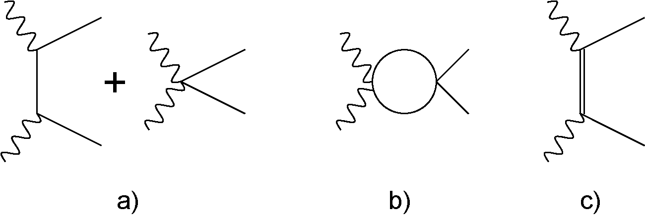
Figure 1: Feynman diagrams for $\gamma\gamma\to\pi\pi$: a) ${\cal O}(p^{2})$ and ${\cal O}(p^{4})$ tree-level (only in the charged channel), b) example of ${\cal O}(p^{4})$ loops, c) vector resonance exchanges (${\cal O}(p^{6})$ and higher in our holographic approach). No other resonance diagram contributes in our analysis. The wavy, solid and double lines stand for photons, pions and vector resonances, respectively.

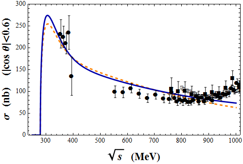
Figure 2: $\gamma\gamma\to\pi^{+}\pi^{-}$ cross section compared to our large-$N_{C}$ expressions. The dashed (orange) line is obtained from the Born term with one-pion exchange, which is ${\cal O}(p^{2})$ in the $\chi$PT counting. In the holographic approach we have also vector exchanges, but their effect is essentially negligible even at high energies. The solid (blue) curve represents the prediction obtained including the Born term + ${\cal O}(p^{4})$ loop + vector exchanges. The data points are from MARK-II (circles) MARK-II , CELLO (filled squares) CELLO , and BELLE experiment (empty squares) charged-BELLE .

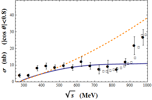
Figure 3: $\gamma\gamma\to\pi^{0}\pi^{0}$ cross section. Data from Crystal Ball CrystalBall:1990 (circles) and BELLE neutral-BELLE (empty squares) are compared to the ${\cal O}(p^{4})$ $\chi$PT expression, which comes only from one-loop diagrams (dashed orange). If we add the resonance contributions from the holographic “Cosh” model, we obtain the solid blue curve. One can appreciate the relevance of the pion loops at low energies, together with the importance of its interference with the vector meson exchanges at higher energy.

The low-energy expansion of the helicity amplitudes for $t=m_{\pi}^{2}$ provides the polarizabilities Gasser:2005 ; Gasser:2006 :

$$\frac{\displaystyle\alpha}{\displaystyle m_{\pi}}H_{++}(s,t=m_{\pi}^{2}) = \frac{\displaystyle\alpha}{\displaystyle m_{\pi}}\,\bigg{[}A^{\gamma\gamma\to\pi\pi}\,\,+\,\,2(4m_{\pi}^{2}-s)B^{\gamma\gamma\to\pi\pi}\,\bigg{]}_{t=m_{\pi}^{2}}$$

$$\,\,\,\stackrel{{\scriptstyle s\to 0}}{{=}}\,\,\, (\alpha_{1}-\beta_{1})\,\,\,+\,\,\,\frac{\displaystyle s}{\displaystyle 12}\,(\alpha_{2}-\beta_{2})\,\,\,+\,\,\,{\cal O}(s^{2})\,,$$

$$\frac{\displaystyle\alpha}{\displaystyle m_{\pi}}H_{+-}(s,t=m_{\pi}^{2}) = \frac{\displaystyle\alpha}{\displaystyle m_{\pi}}\,8m_{\pi}^{2}B^{\gamma\gamma\to\pi\pi}\bigg{|}_{t=m_{\pi}^{2}}$$ (52)

$$\,\,\,\stackrel{{\scriptstyle s\to 0}}{{=}}\,\,\, (\alpha_{1}+\beta_{1})\,\,\,+\,\,\,\frac{\displaystyle s}{\displaystyle 12}\,(\alpha_{2}+\beta_{2})\,\,\,+\,\,\,{\cal O}(s^{2})\,.$$

In the case of the charged pion amplitude, the Born term is subtracted when defining the polarizabilities.

The chiral expansion for the $\gamma\gamma\to\pi^{0}\pi^{0}$ polarizabilities are Gasser:2005 :

$$(\alpha_{1}-\beta_{1})_{\pi^{0}} = \frac{\displaystyle\alpha}{\displaystyle m_{\pi}}\,\frac{\displaystyle 1}{\displaystyle(4\pi F)^{2}}\,\bigg{\{}\,-\,\frac{\displaystyle 1}{\displaystyle 3}\,\,+\,\,\,\left(a_{1}^{r}+8b^{r}+{\cal O}(p^{6})\mbox{ loops}\right)\,\frac{\displaystyle m_{\pi}^{2}}{\displaystyle(4\pi F)^{2}}\,\,+\,\,{\cal O}(m_{\pi}^{4})\bigg{\}}\,,$$

$$(\alpha_{1}+\beta_{1})_{\pi^{0}} = \frac{\displaystyle\alpha}{\displaystyle m_{\pi}}\,\frac{\displaystyle m_{\pi}^{2}}{\displaystyle(4\pi F)^{4}}\,\bigg{\{}\,\left(8b^{r}+{\cal O}(p^{6})\mbox{ loops}\right)\,\,+\,\,{\cal O}(m_{\pi}^{2})\bigg{\}}\,,$$

$$(\alpha_{2}-\beta_{2})_{\pi^{0}} = \frac{\displaystyle\alpha}{\displaystyle m_{\pi}}\,\frac{\displaystyle 1}{\displaystyle m_{\pi}^{2}(4\pi F)^{2}}\,\bigg{\{}\frac{\displaystyle 156}{\displaystyle 45}\,+\,\left(12a_{2}^{r}-24b^{r}+{\cal O}(p^{6})\mbox{ loops}\right)\,\frac{\displaystyle m_{\pi}^{2}}{\displaystyle(4\pi F)^{2}}\,+\,{\cal O}(m_{\pi}^{4})\bigg{\}}\,,$$

$$(\alpha_{2}+\beta_{2})_{\pi^{0}} = \frac{\displaystyle\alpha}{\displaystyle m_{\pi}}\,\frac{\displaystyle 1}{\displaystyle(4\pi F)^{4}}\,\bigg{\{}\,\left({\cal O}(p^{6})\mbox{ loops}\right)\,+\,{\cal O}(m_{\pi}^{2})\bigg{\}}\,,$$ (53)

where the ${\cal O}(m_{\pi}^{4})$ and ${\cal O}(m_{\pi}^{2})$ terms at the end of each equation represent the contributions of ${\cal O}(p^{8})$ and higher in $\chi$PT.

For the $\gamma\gamma\to\pi^{+}\pi^{-}$ polarizabilities one has the chiral expansion Burgi:1996 ; Gasser:2006

$$(\alpha_{1}-\beta_{1})_{\pi^{+}} = \frac{\displaystyle\alpha}{\displaystyle m_{\pi}}\,\frac{\displaystyle 1}{\displaystyle(4\pi F)^{2}}\,\bigg{\{}\,\frac{\displaystyle 2\bar{\ell}_{\Delta}}{\displaystyle 3}\,\,\,+\,\,\,\left(a_{1}^{r}+8b^{r}+{\cal O}(p^{6})\mbox{ loops}\right)\,\frac{\displaystyle m_{\pi}^{2}}{\displaystyle(4\pi F)^{2}}\,\,+\,\,{\cal O}(m_{\pi}^{4})\bigg{\}}\,,$$

$$(\alpha_{1}+\beta_{1})_{\pi^{+}} = \frac{\displaystyle\alpha}{\displaystyle m_{\pi}}\,\frac{\displaystyle m_{\pi}^{2}}{\displaystyle(4\pi F)^{4}}\,\bigg{\{}\,\left(8b^{r}+{\cal O}(p^{6})\mbox{ loops}\right)\,\,+\,\,{\cal O}(m_{\pi}^{2})\bigg{\}}\,,$$

$$(\alpha_{2}-\beta_{2})_{\pi^{+}} = \frac{\displaystyle\alpha}{\displaystyle m_{\pi}}\,\frac{\displaystyle 1}{\displaystyle m_{\pi}^{2}(4\pi F)^{2}}\,\bigg{\{}\,2\,+\,\left(12a_{2}^{r}-24b^{r}+{\cal O}(p^{6})\mbox{ loops}\right)\,\frac{\displaystyle m_{\pi}^{2}}{\displaystyle(4\pi F)^{2}}\,+\,{\cal O}(m_{\pi}^{2})\bigg{\}}\,,$$

$$(\alpha_{2}+\beta_{2})_{\pi^{+}} = \frac{\displaystyle\alpha}{\displaystyle m_{\pi}}\,\frac{\displaystyle 1}{\displaystyle(4\pi F)^{4}}\,\bigg{\{}\,\left({\cal O}(p^{6})\mbox{ loops}\right)\,+\,{\cal O}(m_{\pi}^{2})\bigg{\}}\,,$$ (54)

with $\bar{\ell}_{\Delta}=192\,\pi^{2}(L_{9}(\mu)+L_{10}(\mu))$. Again, the ${\cal O}(m_{\pi}^{4})$ and ${\cal O}(m_{\pi}^{2})$ terms at the end of each equation represent the contributions of ${\cal O}(p^{8})$ and higher in $\chi$PT. Since the $a_{1}$ parameter is out of the reach in our massless quark holographic approach, we focus on the combinations $(\alpha_{1}+\beta_{1})$ and $(\alpha_{2}\pm\beta_{2})$.

At large $N_{C}$, in our holographic approach based on the $m_{\pi}\to 0$ limit, we have:

$$H_{++}(s,t=m_{\pi}^{2}) = \frac{\displaystyle a_{2}}{\displaystyle(4\pi F)^{4}}\bigg{[}\frac{\displaystyle 2s}{\displaystyle 3}\,+\,{\cal O}(s^{2})\bigg{]}\,,$$

$$H_{+-}(s,t=m_{\pi}^{2}) = \frac{\displaystyle b\,m_{\pi}^{2}}{\displaystyle(4\pi F)^{4}}\bigg{[}8\,-\,\frac{\displaystyle 96L_{1}s}{\displaystyle F^{2}}\,+\,{\cal O}(s^{2})\bigg{]}\,.$$ (55)

This leads to the large $N_{C}$ determinations of the polarizabilities,

$$(\alpha_{1}+\beta_{1}) = \frac{\displaystyle\alpha}{\displaystyle m_{\pi}}\,\frac{\displaystyle 8b\,m_{\pi}^{2}}{\displaystyle(4\pi F)^{4}}\,\,+\,\,{\cal O}(m_{\pi}^{3})\,,$$

$$(\alpha_{2}-\beta_{2}) = \frac{\displaystyle\alpha}{\displaystyle m_{\pi}}\,\frac{\displaystyle 8a_{2}}{\displaystyle(4\pi F)^{4}}\,+\,{\cal O}(m_{\pi})\,,$$

$$(\alpha_{2}+\beta_{2}) = \,-\,\frac{\displaystyle\alpha}{\displaystyle m_{\pi}}\,\frac{\displaystyle 1152L_{1}b}{\displaystyle F^{2}}\,\frac{\displaystyle m_{\pi}^{2}}{\displaystyle(4\pi F)^{4}}\,+\,{\cal O}(m_{\pi}^{3})\,,$$ (56)

where we used the holographic prediction $a_{2}=6\,b$. Both the neutral and charged channels have the same structure and one must use the corresponding $a_{2}$ and $b$ parameters. Notice that in the large $N_{C}$ limit the polarizability $(\alpha_{2}+\beta_{2})$ starts at ${\cal O}(p^{8})$. In real world, the leading tree-level ${\cal O}(p^{8})$ contribution obtained here competes with the $1/N_{C}$ suppressed ${\cal O}(p^{6})$ loops.

It is convenient to keep track of the different contributions, and observe at which chiral order each of the polarizabilities begins. The first non-vanishing contribution appears at ${\cal O}(p^{4})$ and comes from one-loop diagrams. Indeed, only $(\alpha_{2}-\beta_{2})$ is different from zero at this order, and the other polarizabilities $(\alpha_{1}+\beta_{1})$ and $\alpha_{2}+\beta_{2})$ vanish Bijnens:1988 ; Burgi:1996 ; Gasser:2005 ; Gasser:2006 . The chiral expansion for $(\alpha_{1}+\beta_{1})$ begins at ${\cal O}(p^{6})$ (loop+tree-level) Burgi:1996 ; Gasser:2005 ; Gasser:2006 . The polarizability $(\alpha_{2}+\beta_{2})$ also starts at this order but only via loops, since the first tree-level contribution appears at ${\cal O}(p^{8})$ Burgi:1996 ; Gasser:2005 ; Gasser:2006 .

At large $N_{C}$ the first contribution to both $(\alpha_{1}+\beta_{1})_{\pi^{0}}$ and $(\alpha_{2}-\beta_{2})_{\pi^{0}}$ starts at ${\cal O}(p^{6})$. The polarizability $(\alpha_{2}+\beta_{2})_{\pi^{0}}$ is even more suppressed at large $N_{C}$, starting at ${\cal O}(p^{8})$. In Table 2 we see how the values of the polarizabilities evolve as we include higher chiral orders. In the first column we provide the one-loop ${\cal O}(p^{4})$ contributions Bijnens:1988 (the ${\cal O}(p^{2})$ pion Born term is explicitly removed in the charged channel definitions and absent in the neutral one). Then we add the lowest order contribution from tree-level resonance exchanges from our holographic Lagrangian, ${\cal O}(p^{6})$ for $(\alpha_{1}+\beta_{1})$ and $(\alpha_{2}-\beta_{2})$ and ${\cal O}(p^{8})$ in the case of $(\alpha_{2}+\beta_{2})$. Finally, in the last column we also sum up the ${\cal O}(p^{6})$ loop contribution. We provide three numbers: the first one is given by $\bar{\ell}_{3}$ and $\bar{\ell}_{4}$ from Gasser:2005 ; Gasser:2006 and the values of $\bar{\ell}_{1,2,\Delta}$ extracted from $L_{1,2,3,9,10}(\mu)$ estimated from the “Cosh” model at $\mu=770$ MeV; the second one is similar but with $\bar{\ell}_{1,2,\Delta}$ estimated from the Hard-Wall model; for the third number (in brackets) we have used the values of the ${\cal O}(p^{4})$ LEC’s from Gasser:2005 ; Gasser:2006 in the ${\cal O}(p^{6})$ loop contribution. In the neutral channel one can see that the resonance contributions seem to be slightly dominant with respect to the ${\cal O}(p^{6})$ loops. However, vector resonance exchanges in the $\gamma\gamma\to\pi^{+}\pi^{-}$ amplitude carry a $\frac{1}{9}$ suppression factor and we found them of the same numerical size as the ${\cal O}(p^{6})$ loops.

In Table 3 we compare the result in the last column of Table 2 to other determinations. In particular, we quote the outcome of dispersive analyses such as the Muskhelishvili-Omnès (MO) relation in terms of the $\pi\pi$–scattering phase-shifts Moussallam:2010 and the Roy-Steiner equations Hoferichter:2011wk , together with the result of the $\chi$PT computation at ${\cal O}(p^{6})$ Gasser:2005 ; Gasser:2006 . We obtain an overall agreement between the holographic determination and the dispersive and chiral computations. Further comparisons can be carried out with previous experimental and theoretical results Pennington-rev collected in Table 4

We remark again that in our computation we have considered the charge matrix Q=diag$(\frac{2}{3},-\frac{1}{3},-\frac{1}{3})$ in the calculation of our large–$N_{C}$ estimates of the LEC’s. Nonetheless, we have found a relatively good numerical agreement with the next-to-next-to-leading order (NNLO) $\chi$PT calculations from Refs. Gasser:2005 ; Gasser:2006 , which rather considered the $SU(2)$ charge matrix Q=diag$(\frac{1}{2},-\frac{1}{2})$.

	${\cal O}(p^{4})$	${\cal O}(p^{4})$	${\cal O}(p^{4})$
		+ resonance	+ reson. (hologr.)
		(hologr.)	+ ${\cal O}(p^{6})$ loops
$(\alpha_{1}+\beta_{1})_{\pi^{0}}$	0	0.58	0.75  ;  0.74  ;  [0.69]
$(\alpha_{2}-\beta_{2})_{\pi^{0}}$	20.73	27.67	30.18  ;  29.98  ;  [34.65]
$(\alpha_{2}+\beta_{2})_{\pi^{0}}$	0	-0.24	-0.16  ;  -0.17  ;  [-0.20]
$(\alpha_{1}+\beta_{1})_{\pi^{+}}$	0	0.06	0.16  ;  0.16  ;  [0.08]
$(\alpha_{2}-\beta_{2})_{\pi^{+}}$	11.96	12.65	14.23  ;  14.12  ;  [17.08]
$(\alpha_{2}+\beta_{2})_{\pi^{+}}$	0	-0.02	0.03  ;  0.02  ;  [-0.02]

Table 2: Polarizabilities in units of $10^{-4}$ fm³ for $\alpha_{1}$, $\beta_{1}$, and $10^{-4}$ fm⁵ for $\alpha_{2}$, $\beta_{2}$. They are provided at ${\cal O}(p^{4})$ in the second column whereas in the third column we add the resonance contribution from the holographic models, which begins at ${\cal O}(p^{6})$ for $(\alpha_{1}+\beta_{1})$ and $(\alpha_{2}-\beta_{2})$, and at ${\cal O}(p^{8})$ in the $\chi$PT expansion for $(\alpha_{2}-\beta_{2})$. The ${\cal O}(p^{6})$ loop contributions are finally added in the last column.

	${\cal O}(p^{4})$	Dispersive	NNLO
	+ reson. (hologr.)	analysis	$\chi$PT
	+ ${\cal O}(p^{6})$ loops	Moussallam:2010 ; Hoferichter:2011wk	Gasser:2005 ; Gasser:2006
$(\alpha_{1}+\beta_{1})_{\pi^{0}}$	0.75  ;  0.74  ;  [0.69]	$1.22\pm 0.12\pm 0.03$	$1.1\pm 0.3$
$(\alpha_{2}-\beta_{2})_{\pi^{0}}$	30.18  ;  29.98  ;  [34.65]	$32.1\pm 0.9\pm 1.9$	$37.6\pm 3.3$
$(\alpha_{2}+\beta_{2})_{\pi^{0}}$	-0.16  ;  -0.17  ;  [-0.20]	$-0.19\pm 0.02\pm 0.01$	0.04
$(\alpha_{1}+\beta_{1})_{\pi^{+}}$	0.16  ;  0.16  ;  [0.08]	$0.19\pm 0.09\pm 0.03$	0.16   [0.16]
$(\alpha_{2}-\beta_{2})_{\pi^{+}}$	14.23  ;  14.12  ;  [17.08]	$14.7\pm 1.5\pm 1.4$	16.2  [21.6]
		$15.3\pm 3.7$
$(\alpha_{2}+\beta_{2})_{\pi^{+}}$	0.03  ;  0.02  ;  [-0.02]	$0.11\pm 0.03\pm 0.01$	-0.001

Table 3: Our holographic predictions for the polarizabilities, provided in the second column (same outcomes as in the last column in Table 2), are compared to the dispersive results from Roy-Steiner equations Hoferichter:2011wk (second value for $(\alpha_{2}-\beta_{2})_{\pi^{+}}$ in the third column) and the MO representation Moussallam:2010 (all the remaining outcomes in the third column). They are also compared to the NNLO $\chi PT$ analyses Gasser:2005 ; Gasser:2006 , provided in the last column. Units are the same as in Table 2.

	CELLO	MARK-II	Crystal	Vector	Sum
			Ball	exchanges	rules
	Kaloshin:1994 ; CELLO	Kaloshin:1994 ; MARK-II	Kaloshin:1994 ; CrystalBall:1990	Ko:1990 ; Babusci:1993	Filkov:2005
$(\alpha_{1}+\beta_{1})_{\pi^{0}}$			$1.00\pm 0.05$	0.83	$0.802\pm 0.035$
$(\alpha_{2}-\beta_{2})_{\pi^{0}}$					$39.72\pm 8.01$
$(\alpha_{2}+\beta_{2})_{\pi^{0}}$					$-0.171\pm 0.067$
$(\alpha_{1}+\beta_{1})_{\pi^{+}}$	$0.30\pm 0.04$	$0.22\pm 0.06$		0.07	$0.166\pm 0.024$
$(\alpha_{2}-\beta_{2})_{\pi^{+}}$					$25.75\pm 7.03$
$(\alpha_{2}+\beta_{2})_{\pi^{+}}$					$0.121\pm 0.064$

Table 4: Pion polarizabilities from experimental measurements Kaloshin:1994 ; CELLO ; MARK-II ; CrystalBall:1990 and theoretical analyses Ko:1990 ; Babusci:1993 ; Filkov:2005 . Units are the same as in Table 2.

5 Conclusions

Following previous analyses Son:2010vc ; Colangelo:2012ip , we have determined a novel set of relations between QCD matrix elements using holographic models where chiral symmetry is broken through IR b.c.’s. We have focused on the scattering amplitudes of pions and photons, finding that the three processes $\pi\pi\to\pi\pi$, $\gamma\gamma\to\pi\pi$ and $\gamma\to\pi\pi\pi$ involve a single scalar function $h(Q^{2})$. This function is given by a suitable 5D integral of the EoM Green’s function and accepts the usual decomposition in terms of resonance exchanges. Furthermore, in the considered processes only the vector mesons contribute (scalars and resonances of spin $S\geq 2$ are not included in the present approach).

In a detailed phenomenological analysis of $\gamma\gamma\to\pi\pi$ we have found an overall agreement with the experimental cross section for a broad range of energy. Likewise, the computed polarizabilities at low energies show a fair agreement between the holographic approach, previous computations and experiment.

Appendix A Constraints on the background functions

Here we provide constraints on the background functions $f^{2}(z)$ and $g^{2}(z)$. As proposed in ref. Son:2003et , these functions must be invariant under the reflection of $z$ in order to properly define the parity. More constraints come from the results for the low-energy constants.

With the resonance decomposition of the gauge potential (7), up to ${\cal O}(p^{4})$ the 5D Yang-Mills action reduces to the $\chi PT$ Lagrangian Hirn:2005nr ; Sakai:2004cn ; Colangelo:2012ip :

$$S_{2}[\pi]+S_{4}[\pi] = \displaystyle{\int}d^{4}x\,\bigg{[}\frac{F^{2}}{4}<u_{\mu}u^{\mu}>$$ (57)

$$\qquad\qquad+L_{1}<u_{\mu}u^{\mu}>^{2}+L_{2}<u_{\mu}u_{\nu}><u^{\mu}u^{\nu}>+L_{3}<u_{\mu}u^{\mu}u_{\nu}u_{\nu}>$$

$$\qquad\qquad-iL_{9}<f_{+\mu\nu}u^{\mu}u^{\nu}>+\frac{L_{10}}{4}<f_{+\mu\nu}f_{+}^{\mu\nu}-f_{-\mu\nu}f_{-}^{\mu\nu}>$$

$$\qquad\qquad+\frac{H_{1}}{2}<f_{+\mu\nu}f_{+}^{\mu\nu}+f_{-\mu\nu}f_{-}^{\mu\nu}>\,\bigg{]}\,.$$

The low-energy constants in (57) are given by the 5D integrals

$$F^{2} = 4\left(\int_{-z_{0}}^{z_{0}}\frac{\mathrm{d}z}{f^{2}(z)}\right)^{-1}\,,$$

$$L_{1} = \frac{1}{2}L_{2}=-\frac{1}{6}L_{3}=\frac{1}{32}\int_{-z_{0}}^{z_{0}}\frac{(1-\psi_{0}^{2})^{2}}{g^{2}(z)}\,\mathrm{d}z\,,$$

$$L_{9} = -L_{10}=\frac{1}{4}\int_{-z_{0}}^{z_{0}}\frac{1-\psi_{0}^{2}}{g^{2}(z)}\,\mathrm{d}z\,,$$ (58)

$$H_{1} = -\frac{1}{8}\int_{-z_{0}}^{z_{0}}\frac{1+\psi_{0}^{2}}{g^{2}(z)}\,\mathrm{d}z\,.$$

We demand that all these integrals except $H_{1}$ are finite. For $H_{1}$, which is the coefficient of the kinetic term of the external sources, we require it to be divergent. From the finiteness of the pion decay constant $F$ we find the solution

$$\psi_{0}(z)=\frac{F^{2}}{2}\int_{0}^{z}\frac{1}{f^{2}(z)}\mathrm{d}z\,\,\,,$$ (59)

which satisfies the equation of motion with boundary conditions $\psi_{0}(\pm z_{0})=\pm~{}1$. Since $\psi_{0}(z)$ is a monotonic function of $z$, we can choose it as the coordinate parameter through a coordinate transformation in $z$. Defining $y=\psi_{0}(z)$, it is not difficult to find the new background functions

$${\tilde{f}}^{2}(y)=\frac{F^{2}}{2},\,\,\,\,{\tilde{g}}^{2}(y)=\frac{F^{2}}{2}\frac{g^{2}(z(y))}{f^{2}(z(y))},$$ (60)

together with the boundaries $y=\pm 1$. It turns out that this coordinate system is convenient in many respects, both for theoretical derivations and numerical calculations. In this coordinate system the integral for $F$ becomes trivial, and the other integrals can be expressed as

$$L_{1} = \frac{1}{32}\int_{-1}^{1}\frac{(1-y^{2})^{2}}{{\tilde{g}}^{2}(y)}\,\mathrm{d}y\,\,,$$

$$L_{9} = \frac{1}{4}\int_{-1}^{1}\frac{1-y^{2}}{{\tilde{g}}^{2}(y)}\,\mathrm{d}y\,\,,$$ (61)

$$H_{1} = -\frac{1}{8}\int_{-1}^{1}\frac{1+y^{2}}{{\tilde{g}}^{2}(y)}\,\mathrm{d}y\,\,.$$

Requiring that $L_{1}$ and $L_{9}$ are finite and $H_{1}$ divergent, we get the constraint near the boundaries

$$(1-y^{2})^{2}<{\tilde{g}}^{2}(y)\leq C(1-y^{2})$$ (62)

with $C$ a constant. Actually, the explicit boundary behavior of the function, ${\tilde{g}}^{2}(y)$, can be used to clarify the ultraviolet property of different models. Among the models shown in the next appendix, this function behaves as $(1-y^{2})^{0}$ in the flat model, related to a convergent value of $H_{1}$, while in the Sakai-Sugimoto model, it goes as $(1-y^{2})^{4/3}$. As for all the asymptotic anti-de Sitter backgrounds, the equality in the above relation is exactly satisfied, e.g., in the “cosh” and Hard-Wall models.

In the new coordinate system, the quantity $\mathcal{H}$ defined in Eq. (28) simplifies as

$$\mathcal{H}=\frac{1}{4}\int_{-1}^{1}~{}{\tilde{g}}^{2}(y)\,\mathrm{d}y\,\,,$$ (63)

and, with the constraint (62), it is finite.

Appendix B Holographic models

We have used four different holographic models, defined by the functions $f^{2}(z)$ and $g^{2}(z)$ and by the value of $z_{0}$. Here we list their details in each model. The expressions of the wave functions solutions of the equation of motion, and of other quantities like $F$, the couplings and the mass spectrum, can be found in the appendix of ref. Colangelo:2012ip .

“Flat” background Son:2003et :

$$f^{2}(z)=\frac{\Lambda^{2}}{g_{5}^{2}}\,\,\,,~{}~{}g^{2}(z)=g_{5}^{2}\,\,\,\ ,~{}~{}z_{0}=1.$$ (64)

“Cosh” model  Son:2003et :

$$f^{2}(z)=\frac{\Lambda^{2}\cosh^{2}(z)}{g_{5}^{2}}\,\,\,,~{}~{}g^{2}(z)=g_{5}^{2}\,\,\,,~{}~{}z_{0}=\infty.$$ (65)

“Hard-wall" model Hirn:2005nr :

$$f^{2}(z)=\frac{1}{g_{5}^{2}(z_{0}-|z|)}\,\,\,,~{}~{}g^{2}(z)=g_{5}^{2}(z_{0}-|z|)\,\,\,,~{}~{}z_{0}<\infty.$$ (66)

“Sakai-Sugimoto" model Sakai:2004cn ; Sakai:2005yt :

$$f^{2}(z)=\frac{\Lambda^{2}(1+z^{2})}{g_{5}^{2}}\,\,\,,~{}~{}g^{2}(z)=g_{5}^{2}(1+z^{2})^{1/3}\,\,\,,~{}~{}z_{0}=\infty.$$ (67)

Appendix C Isospin and partial-wave projection in $\pi\pi$–scattering

The amplitude $A(s,t,u)$ provides the scattering amplitudes $T^{I}$ of modes with definite isospin $I=0,1,2$ op4-chpt ; op6-pipi-scat :

$$T^{0}(s,t,u) = 3A(s,t,u)+A(t,s,u)+A(u,s,t)\,,$$

$$T^{1}(s,t,u) = A(t,s,u)-A(u,s,t)\,,$$

$$T^{2}(s,t,u) = A(t,s,u)+A(u,s,t)\,.$$ (68)

In the isospin $I=2$ amplitude, there are no resonances in the s–channel, only exchanges in the crossed channels. This simplifications makes the amplitude particularly interesting for the study of its partial waves, which in the massless quark limit have the form op4-chpt ; op6-pipi-scat

$$T^{I}_{J}(s) = \frac{\displaystyle 1}{\displaystyle 32\pi s}\displaystyle{\int}_{-s}^{0}{\rm dt}\,\,P_{J}\bigg{(}1+\frac{2t}{s}\bigg{)}\,T^{I}(s,t,u)$$

$$\,\,\,=\,\,\,\frac{\displaystyle 1}{\displaystyle 64\pi}\displaystyle{\int}_{-1}^{1}{\rm dx}\,\,P_{J}(x)\,T^{I}(s,-s(1-x)/2,-s(1+x)/2)$$

$$\,\,\,=\,\,\,\frac{\displaystyle 1}{\displaystyle 32\pi}\displaystyle{\int}_{0}^{1}{\rm dy}\,\,P_{J}(1-2y)\,T^{I}(s,-sy,-s(1-y))\,,$$

with $u=-s-t$ (in the chiral limit), $y=(1-x)/2=-t/s$ and $P_{J}$ the Legendre polynomials.

Appendix D Expressions for the relevant ${\cal O}(p^{6})$ LEC’s

Here we provide the expressions of some ${\cal O}(p^{6})$ LEC’s derived in ref. Colangelo:2012ip , which have been used in the calculation of the polarizabilities. They are summarized in Table 5, where the following definitions have been used:

$$S_{VV}=\sum_{n=1}^{\infty}\frac{a_{Vv^{n}}^{2}}{m_{v^{n}}^{2}}\,,\qquad S_{V\pi\pi}=\sum_{n=1}^{\infty}\frac{a_{Vv^{n}}b_{v^{n}\pi\pi}}{m_{v^{n}}^{2}}\,,\qquad S_{AA}=\sum_{n=1}^{\infty}\frac{a_{Aa^{n}}^{2}}{m_{a^{n}}^{2}}\,.$$ (70)

The coupling $a_{Aa^{n}}$ comes from the interaction

$$S_{\rm{YM}}\bigg{|}_{{\rm 1-res.}}\supset\qquad\,\langle\,\frac{f^{\mu\nu}_{-}}{2}(\nabla_{\mu}a_{\nu}^{n}-\nabla_{\nu}a_{\mu}^{n})a_{Aa^{n}}\,\rangle,$$ (71)

with $f_{-}^{\alpha\beta}=\xi_{L}^{\dagger}F_{L}^{\alpha\beta}\xi_{L}-\xi_{R}^{\dagger}F_{R}^{\alpha\beta}\xi_{R}$. The explicit contributions given in terms of $F$ and $N_{C}$ come from the diagrams with two parity-odd vertices, while the other terms come from diagrams with two even-parity vertices. From the expressions in Tab. 5 one easily recovers the results (33), (38), (41) and (43).

$C_{53}$	$\frac{3}{16}S_{AA}-\frac{1}{16}S_{V\pi\pi}-\frac{3}{16}S_{VV}+\frac{N_{C}^{2}}{3072\pi^{4}F^{2}}$
$C_{55}$	$-\frac{3}{16}S_{AA}+\frac{1}{16}S_{V\pi\pi}+\frac{3}{16}S_{VV}+\frac{N_{C}^{2}}{3072\pi^{4}F^{2}}$
$C_{56}$	$-\frac{3}{8}S_{AA}-\frac{1}{8}S_{V\pi\pi}+\frac{3}{8}S_{VV}-\frac{N_{C}^{2}}{1536\pi^{4}F^{2}}$
$C_{57}$	$-\frac{1}{8}S_{AA}+\frac{1}{4}S_{V\pi\pi}+\frac{1}{8}S_{VV}$
$C_{59}$	$\frac{1}{4}S_{AA}-\frac{1}{16}S_{V\pi\pi}-\frac{1}{4}S_{VV}-\frac{N_{C}^{2}}{3072\pi^{4}F^{2}}$
$C_{78}$	$-\frac{1}{4}S_{AA}+\frac{1}{16}S_{V\pi\pi}+\frac{1}{4}S_{VV}$
$C_{87}$	$-\frac{1}{8}S_{AA}+\frac{1}{8}S_{VV}$
$C_{88}$	$-\frac{1}{8}S_{V\pi\pi}$

Table 5: Holographic predictions for some of the ${\cal O}(p^{6})$ LEC’s in the even sector Colangelo:2012ip .

Appendix E Contribution to $\gamma\gamma\to\pi\pi$ from ${\cal O}(p^{4})$ diagrams

In the neutral channel $\gamma\gamma\to\pi^{0}\pi^{0}$, the only ${\cal O}(p^{4})$ contribution appears at the one loop level Bijnens:1988 ; Gasser:2005 :

$$\Delta A(s,t,u)^{\gamma\gamma\to\pi^{0}\pi^{0}}_{\rm{\cal O}(p^{4})} = \frac{\displaystyle 4\bar{G}_{\pi}(s)}{\displaystyle F_{\pi}^{2}}\,\bigg{(}1-\frac{\displaystyle m_{\pi}^{2}}{\displaystyle s}\bigg{)}\,,$$

$$\Delta B(s,t,u)^{\gamma\gamma\to\pi^{0}\pi^{0}}_{\rm{\cal O}(p^{4})} = 0\,,$$ (72)

with

$$\bar{G}_{\pi}(s) = -\,\frac{\displaystyle 1}{\displaystyle 16\pi^{2}}\,\bigg{[}\,1\,+\,\frac{\displaystyle m_{\pi}^{2}}{\displaystyle s}\,\bigg{(}\ln\frac{\displaystyle\rho_{\pi}+1}{\displaystyle\rho_{\pi}-1}\bigg{)}^{2}\,\bigg{]}\,,$$ (73)

given by the phase-space factor $\rho_{\pi}=\sqrt{1-4m_{\pi}^{2}/s}$.

In the $\gamma\gamma\to\pi^{+}\pi^{-}$ channels the ${\cal O}(p^{4})$ diagrams contribute both at one loop and tree-level Bijnens:1988 ; Gasser:2006 :

$$\Delta A(s,t,u)^{\gamma\gamma\to\pi^{+}\pi^{-}}_{\rm{\cal O}(p^{4})} = \frac{\displaystyle 2\bar{G}_{\pi}(s)}{\displaystyle F_{\pi}^{2}}\,\,\,+\,\,\,\frac{\displaystyle\bar{\ell}_{\Delta}}{\displaystyle 24\pi^{2}F_{\pi}^{2}}\,,$$

$$\Delta B(s,t,u)^{\gamma\gamma\to\pi^{+}\pi^{-}}_{\rm{\cal O}(p^{4})} = 0\,,$$ (74)

with the tree-level term $\bar{\ell}_{\Delta}=\bar{\ell}_{6}-\bar{\ell}_{5}=192\pi^{2}(\ell_{5}(\mu)-\ell_{6}(\mu)/2)$. However, in the type of holographic models studied in this work one always has $\ell_{5}-\ell_{6}/2=L_{10}+L_{9}=0$ at large $N_{C}$ Hirn:2005nr ; Sakai:2005yt .

References

- (1) D. T. Son and N. Yamamoto, [arXiv:1010.0718].
- (2) P. Colangelo, F. De Fazio, J.J. Sanz-Cillero, F. Giannuzzi, and S. Nicotri, Phys. Rev. D85 (2012) 035013 [arXiv:1108.5945].
- (3) L. Cappiello, O. Catá, and G. D’Ambrosio, Phys. Rev. D82 (2010) 095008 [arXiv:1004.2497].
- (4) M. Knecht, S. Peris, and E. de Rafael, JHEP 1110 (2011) 048 [arXiv:1101.0706].
- (5) S.K. Domokos, J.A. Harvey, and A.B. Royston, JHEP 1105 (2011) 107 [arXiv:1101.3315].
- (6) R. Alvares, C. Hoyos, and A. Karch, Phys. Rev. D84 (2011) 095020 [arXiv:1108.1191].
- (7) A. Gorsky, P.N. Kopnin, A. Krikun, and A. Vainshtein, Phys. Rev. D85 (2012) 086006 [arXiv:1201.2039].
- (8) I. Iatrakis and E. Kiritsis, JHEP 1202 (2012) 064 [arXiv:1109.1282].
- (9) P. Colangelo, J.J. Sanz-Cillero, and F. Zuo, JHEP 1211 (2012) 012 [arXiv:1207.5744].
- (10) D. T. Son and M. A. Stephanov, Phys. Rev. D69 (2004) 065020 [arXiv:hep-ph/0304182].
- (11) T. Sakai and S. Sugimoto, Prog. Theor. Phys. 113 (2005) 843 [arXiv:hep-th/0412141].
- (12) J. Hirn and V. Sanz, JHEP 12 (2005) 030 [arXiv:hep-ph/0507049].
- (13) T. Sakai and S. Sugimoto, Prog. Theor. Phys. 114 (2005) 1083 [arXiv:hep-th/0507073].
- (14) G. ’t Hooft, Nucl. Phys. B72 (1974) 461; 75 (1974) 461. E. Witten, Nucl. Phys.B160 (1979) 57.
- (15) S. Weinberg, Physica A 96 (1979) 327.
- (16) J. Gasser and H. Leutwyler, Annals Phys. 158 (1984) 142; Nucl. Phys. B 250 (1985) 465, 517.
- (17) J. Bijnens, G. Colangelo, and G. Ecker, JHEP 02 (1999) 020 [arXiv:hep-ph/9902437].
- (18) J. Bijnens, G. Colangelo, and G. Ecker, Annals Phys. 280 (2000) 100 [arXiv:hep-ph/9907333].
- (19) J. Bijnens, L. Girlanda, and P. Talavera, Eur. Phys. J. C23 (2002) 539-544, [arXiv:hep-ph/0110400].
- (20) T. Ebertshauser, H.W. Fearing, and S. Scherer, Phys. Rev. D65 (2002) 054033, [arXiv:hep-ph/0110261].
- (21) U. Burgi, Nucl.Phys. B 479 (1996) 392 [arXiv:hep-ph/9602429]; Phys.Lett. B 377 (1996) 147 [arXiv:hep-ph/9602421].
- (22) J. Gasser, M. A. Ivanov, and M. E. Sainio, Nucl. Phys. B728 (2005) 31 [arXiv:hep-ph/0506265].
- (23) J. Gasser, M. A. Ivanov, and M. E. Sainio, Nucl. Phys. B745 (2006) 84 [arXiv:hep-ph/0602234].
- (24) J. Bijnens and F. Cornet, Nucl. Phys. B296 (1988) 557.
- (25) J. Wess and B. Zumino, Phys. Lett. B37 (1971) 95.
- (26) E. Witten, Nucl. Phys. B223 (1983) 422, 433.
- (27) G. Ecker, J. Gasser, A. Pich and E. de Rafael, Nucl. Phys. B321 (1989) 311. G. Ecker, J. Gasser, H. Leutwyler, A. Pich and E. de Rafael, Phys. Lett. B223 (1989) 425.
- (28) V. Cirigliano, G. Ecker, M. Eidemüller, R. Kaiser, A. Pich and J. Portolés, Nucl. Phys. B753 (2006) 139 [arXiv:hep-ph/0603205].
- (29) J. Beringer et al. [Particle Data Group Collaboration], Phys. Rev. D86 (2012) 010001.
- (30) J. Bijnens, P. Dhonte and P. Talavera, JHEP 0401 (2004) 050. [arXiv:hep-ph/0401039].
- (31) Z.H. Guo, J.J. Sanz-Cillero and H.Q. Zheng, Phys. Lett. B661 (2008) 342 [arXiv:0710.2163 [hep-ph]].
- (32) J. Nieves, A. Pich and E. Ruiz Arriola, Phys. Rev D84 (2011) 096001 [arXiv:1107.3247 [hep-ph]].
- (33) P. Ko, Phys. Rev. D41 (1990) 1531.
- (34) D. Babusci, S. Bellucci, G. Giordano, G. Matone, Phys. Lett. B314 (1993) 112.
- (35) J. Bijnens, A. Bramon and F. Cornet, Phys. Lett. B 237 (1990) 488
- (36) T. Hannah, Nucl. Phys. B 593 (2001) 577 [arXiv:hep-ph/0102213]; O. Strandberg, [arXiv:hep-ph/0302064].
- (37) M. Hoferichter, B. Kubis and D. Sakkas, Phys. Rev. D 86 (2012) 116009 [arXiv:1210.6793 [hep-ph]].
- (38) J. Boyer et al. (MARK-II Coll.), Phys. Rev. D 42 (1990) 1350.
- (39) H.J. Behrend et al. (CELLO Coll.), Z. Phys. C 56 (1992) 381.
- (40) H. Marsiske et al. (Crystal Ball Collaboration), Phys. Rev. D41 (1990) 3324.
- (41) T. Mori et al. (Belle Collaboration), J. Phys. Soc. Jpn. 76 (2007) 074102 [arXiv:0704.3538]; T. Mori et al. (Belle Collaboration), Phys. Rev. D 75 (2007) 051101 [arXiv:hep-ex/0610038].
- (42) S. Uehara et al. (Belle Collaboration), Phys. Rev. D 78 (2008) 052004 [arXiv:0805.3387]; S. Uehara et al. (Belle Collaboration), Phys. Rev. D 79 (2009) 052009 [arXiv:0903.3697].
- (43) For a review see: J. Portoles and M. R. Pennington, in Maiani, L. (ed.) et al.: The second DAPHNE physics handbook, vol. 2 579-596 [arXiv:hep-ph/9407295].
- (44) R. Garcia-Martin and B. Moussallam, Eur. Phys. J. C70 (2010) 155 [arXiv:1006.5373].
- (45) M. Hoferichter, D. R. Phillips and C. Schat, Eur. Phys. J. C 71 (2011) 1743 [arXiv:1106.4147 [hep-ph]].
- (46) L. V. Filikov, V. L. Kashevarov, Phys. Rev. C72 (2005) 035211 [arXiv:nucl-th/0505058]; Phys. Rev. C73 (2006) 035210 [arXiv:nucl-th/0512047].
- (47) A.E. Kaloshin, V.M. Persikov and V.V. Serebryakov, Phys. Atom. Nucl. 57 (1994) 2207; Yad. Fiz. 57 N 12 (1994) 2298 [arXiv:hep-ph/9402220]. A.E. Kaloshin and V.V. Serebryakov, Z. Phys. C 64 (1994) 689 [arXiv:hep-ph/9306224].