Structure formation of surfactant membranes under shear flow

Abstract

Shear-flow-induced structure formation in surfactant-water mixtures is investigated numerically using a meshless-membrane model in combination with a particle-based hydrodynamics simulation approach for the solvent. At low shear rates, uni-lamellar vesicles and planar lamellae structures are formed at small and large membrane volume fractions, respectively. At high shear rates, lamellar states exhibit an undulation instability, leading to rolled or cylindrical membrane shapes oriented in the flow direction. The spatial symmetry and structure factor of this rolled state agree with those of intermediate states during lamellar-to-onion transition measured by time-resolved scatting experiments. Structural evolution in time exhibits a moderate dependence on the initial condition.

I Introduction

Surfactant molecules in water self-assemble into various structures such as micelles and bilayer membranes, which display a rich variety of rheological properties under flow. Larson (1999) Even if a basic structure remains to be a bilayer membrane, its mesoscale structure can assume several different states, such as fluid $L_{\alpha}$ or ripple $P_{\beta}$ phase. Under shear flow, lamellae can be oriented parallel or perpendicular to the shear-gradient direction. Diat and Roux first discovered 20 years ago closely-packed multi-lamellar vesicle (MLV) structures, so-called the onion phase, in nonionic surfactant-water mixtures under shear flow. Diat et al. (1993); Roux et al. (1993); Diat et al. (1994) In the last two decades, this onion structure has been studied experimentally using light, Diat et al. (1993, 1994); Courbin et al. (2002); Koschoreck et al. (2009); Suganuma et al. (2010); Fujii et al. (2012) neutron, Diat et al. (1993, 1994); Nettesheim et al. (2003) and X-ray scattering, Suganuma et al. (2010); Ito et al. (2011); Fujii et al. (2012) and also by freeze-fracture electron microscopy, Courbin et al. (2002) and the rheo-NMR method. Medronho et al. (2008); Medronho et al. (2010a, b) Its rheology has been of large interest. Roux et al. (1993); Richtering (2001); Nettesheim et al. (2003); Miyazawa and Tanaka (2007); Koschoreck et al. (2009); Fujii et al. (2012) Typically, a critical shear rate $\dot{\gamma}_{c}$ separates the lamellae and onion phases, where the latter phase consists of mono-disperse onions containing hundreds of lamellar layers. The onion radius $R(\dot{\gamma})$ is reversible and can be described by a unique decreasing function of the shear rate $\dot{\gamma}$. Medronho et al. (2005)

Time-resolving small-angle neutron scattering experiments have revealed that a two-dimensional intermediate structure is formed during the lamellar-to-onion transition with increasing shear rate. Nettesheim et al. (2003) A cylindrical or wavy lamellar structure was speculated to be the transient intermediate structure, but could not be distinguished from the scattering pattern alone. Recent small-angle X-ray scattering experiments with increasing temperature at constant shear rate also indicate a similar pattern around the lamellar-to-onion transition. Ito et al. (2011) Thus, there are some experimental evidences of a transient state, but its structure is still under debate. An alternative experimental approach to gain insight into the structural changes is to characterize defects observed in the lamellar state for moderate shear rates, both in surfactant membranes Medronho et al. (2010b); Medronho et al. (2011) and in thermotropic liquid crystals. Fujii et al. (2010, 2011) It is also worth mentioning that stable cylindrical structures on a ten-micrometer length scale are observed when strong shear flow is applied in the lamellar-sponge coexistence state. Miyazawa and Tanaka (2007)

Several theoretical attempts have been made to tackle this complex problem of structural evolution under shear flow, which consider either instability of the lamellar phase due to undulations Zilman and Granek (1999); Marlow and Olmsted (2002) or the break-up of droplets. van der Lindern et al. (1996); van der Linden and Dröge (1993) Recently, a “dynamical” free energy of MLV under shear flow has been proposed, Lu (2012) which takes into account the slow modes induced by the solvent between the membranes together with their bending and stretching forces. The scaling relations for the MLV size and the terminal shear rate are predicted in agreement with the experiments of Refs. Diat et al., 1993; Roux et al., 1993. In these theories, while the hydrodynamic effects of the solvent are taken into account, the analysis is performed for geometrically simple structures, asp spherical onions or planar lamellae. Thus, the kinetic process of the transformation from the lamellar to the onion phase could not be investigated theoretically so far. In this paper, we study the detailed structural evolution of surfactant membranes under simple shear flow using large-scale particle simulations.

A few simulations have been performed for the formation of lamellar phases in shear flow, while onion formation has never been addressed so far. Oriented lamellae have been obtained in simulations of a coarse-grained molecular model for lipids, Guo et al. (2002); Soddemann et al. (2004); Guo and Kremer (2007) while defect dynamics has been investigated in simulations of a phase-field model of a smectic-A system. Henrich et al. (2012) Onion and intermediate states have large-scale structures of the order of micrometers, which are beyond typical length scales accessible to molecular dynamics (MD) simulations of coarse-grained surfactant molecules. In our study, we employ a meshless-membrane model, Noguchi (2009); Noguchi and Gompper (2006a, b); Shiba and Noguchi (2011) where a membrane particle represents not a surfactant molecule but rather a patch of bilayer membrane – in order to capture the membrane dynamics on a micrometer length scale. This model is well suitable to study membrane dynamics accompanied by topological changes. Alternatively, membranes can be modeled as triangulated surfaces, Noguchi (2009); Gompper and Kroll (2004); Fedosov et al. which require however discrete bond reconnections to describe topological changes. Gompper and Kroll (1998, 2004); Peltomäki et al. (2012) After the first meshless-membrane model was proposed in 1991, Drouffe et al. (1991) several meshless-membrane models have been developed. Noguchi and Gompper (2006a, b); Shiba and Noguchi (2011); Del Pópolo and Ballone (2008); Kohyama (2009); Yuan et al. (2010); Pasqua et al. (2010) In contrast to other meshless-membrane approaches, our models Noguchi and Gompper (2006a, b); Shiba and Noguchi (2011) are capable of separately controlling the membrane bending rigidity $\kappa$ and the line tension $\Gamma$ of membrane edges. Previously, Noguchi (2009); Noguchi and Gompper (2006b) we have combined our meshless-membrane model with multi-particle collision (MPC) dynamics, Kapral (2008); Gompper et al. (2009) a particle-based hydrodynamic simulation technique. With MPC, the hydrodynamic interactions are properly taken into account, but due to the frictional coupling of membrane and solvent, solvent particles can penetrate through the membrane. We here extend the meshless-membrane model into explicit solvent simulation model, in which the fluid particles interact with each other and with the membrane via short-ranged repulsive potentials, so that the solvent can hardly penetrate the membrane, and simulate it with dissipative particle dynamics (DPD), another hydrodynamics simulation technique.

The simulation model and methods are introduced in Sec. II. Then basic membrane properties, including bending rigidity and line tension, are described in Sec. III. In Sec. IV, structure formation in surfactant-water mixtures under shear flow is investigated for variety of shear rates $\dot{\gamma}$ and membrane volume fractions $\varphi$. At high $\dot{\gamma}$ and high $\varphi$, a novel structure of rolled-up membranes is found, which are oriented in the flow direction. A summary and some perspectives are given in Sec. V.

II Model and Methods

II.1 Coarse-Grained Model and Interaction Potentials

To simulate the structure formation in surfactant-membranes systems, we employ a meshless-membrane model with explicit solvent. In this model, two types of particles $\mathcal{A}$ and $\mathcal{B}$ are employed, which denote membrane and solvent particles, respectively. The number of these particles is $N_{\mathcal{A}}$ and $N_{\mathcal{B}}$, which defines the particle density $\phi=(N_{\mathcal{A}}+N_{\mathcal{B}})/V$ – where $V$ is the volume of the simulation box – and the membrane volume fraction $\varphi=N_{\mathcal{A}}/(N_{\mathcal{A}}+N_{\mathcal{B}})$. The particles interact via a potential $U$, which consists of repulsive, attractive, and curvature interactions, $U_{\rm rep},\ U_{\rm att},$ and $U_{\alpha}$, respectively,

$$\frac{U}{k_{\rm B}T}=\sum_{i<j}U_{\rm rep}+\sum_{i\in\mathcal{A}}\epsilon U_{\rm att}+k_{\alpha}U_{\alpha}.$$ (1)

Here, the former sum for repulsive interactions is taken over all pairs of particles, the latter only over the membrane particles.

All neighbor particle pairs interact via the short-ranged repulsive potential

$$U_{\rm rep}=\left\{\begin{array}[]{ll}\epsilon_{c}\left(\frac{\sigma}{r_{ij}}\right)^{12}-B&(r_{ij}<r_{c}^{\rm rep})\\ 0&(r_{ij}\geq r_{c}^{\rm rep})\end{array}\right.$$ (2)

where $r_{ij}$ is the distance between particles $i$ and $j$. This potential is cut off at a distance $r_{c}^{\rm rep}=3.2\sigma$. The length $\sigma$, representing the particle diameter, is employed as the length unit. The constant $B$ is chosen such as to ensure the continuity of the potential at $r=r_{c}^{\rm rep}$. The (dimensionless) potential strength is set to $\epsilon_{c}=4$.

To favor the assembly of membrane particles into smoothly curved sheets in three-dimensional (3D) space, membrane particles interact via the additional potentials $U_{\rm att}$ and $U_{\alpha}$, which have been introduced in the implicit-solvent version of the model previously. Noguchi and Gompper (2006a, b); Shiba and Noguchi (2011) With these potentials, the membranes particles self-assemble into a single-layer sheet, which is a model representation of a bilayer membrane. Here, the attractive interaction is given by

$$U_{\rm att}=0.25\ln\{1+\exp[-4(\rho_{i}-\rho^{*})]\}-C,$$ (3)

which is a function of the local density $\rho_{i}$ of the membrane particles defined by

$$\rho_{i}=\sum_{i\in\mathcal{A}}f_{\rm cut}(r_{ij}/\sigma).$$ (4)

$C=0.25\ln[1+\exp(4\rho^{*})]$ is chosen such that $U_{\rm att}(0)=0$. The cutoff function $f_{\rm cut}$ in Eq. (4) is a $C^{\infty}$ function represented as

$$f_{\rm cut}(s)=\left\{\begin{array}[]{ll}\exp\left[a(1+\frac{1}{(|s|/s_{\rm cut})^{n}-1})\right]&(s<s_{\rm cut})\\ 0&(s\geq s_{\rm cut})\end{array}\right.$$ (5)

where $n=12$, $a=\ln(2)\{(s_{\rm{cut}}/s_{\rm{half}})^{n}-1\}$ with $s_{\rm cut}=2.1$ and $s_{\rm{half}}=1.8$ are used. We set $\rho^{*}=6$ to study a fluid membrane in an explicit solvent.

The curvature potential

$$U_{\alpha}=\sum_{i\in\mathcal{A}}\alpha_{\rm pl}(\bm{r}_{i})$$ (6)

is introduced to incorporate the membrane bending rigidity. Here, the aplanarity $\alpha_{\rm pl}$ provides a measure for the degree of deviation of membrane particle alignment from a planar reference state. It is defined by

$$\alpha_{\rm pl}=\frac{9D_{\rm w}}{T_{\rm w}M_{\rm w}}=\frac{9\lambda_{1}\lambda_{2}\lambda_{3}}{(\lambda_{1}+\lambda_{2}+\lambda_{3})(\lambda_{1}\lambda_{2}+\lambda_{2}\lambda_{3}+\lambda_{3}\lambda_{1})},$$ (7)

where $\lambda_{1}\leq\lambda_{2}\leq\lambda_{3}$ are the three eigenvalues of the local gyration tensor $a_{\alpha\beta}$ of the membrane near particle $i$, which is defined as $a_{\alpha\beta}=\sum_{j\in\mathcal{A}}(\alpha_{j}-\alpha_{G})(\beta_{j}-\beta_{G})w_{\rm cv}(r_{ij})$, with $\alpha,\beta\in\{x,y,z\}$. Here, $\bm{r}_{G}=\sum_{j\in\mathcal{A}}\bm{r}_{j}w_{\rm cv}(r_{ij})/\sum_{j\in\mathcal{A}}w_{\rm cv}(r_{ij})$ is the locally weighted center of mass, and $w_{\rm cv}(r_{ij})$ is a truncated Gaussian function

$$w_{\rm cv}(r_{ij})=\left\{\begin{array}[]{ll}\exp\left(\frac{(r_{ij}/r_{\rm ga})^{2}}{(r_{ij}/r_{\rm cc})^{n}-1}\right)&(r_{ij}<r_{\rm cc})\\ 0&(r_{ij}\geq r_{\rm cc})\end{array}\right.$$ (8)

which is smoothly cut off at $r_{ij}=r_{\rm cc}$. The constants are set as $n=12,\ r_{\rm ga}=1.5\sigma$, and $r_{\rm cc}=3.2\sigma$.

In all our simulations, the volume is chosen such that the number density $\phi$ of the particles is constant,

$$\phi=N/V=0.64\sigma^{-3},\ N=N_{\mathcal{A}}+N_{\mathcal{B}}.$$ (9)

For higher solvent densities, the system is closer to the melting point, and strong attractive interaction between membranes sheets have been found (see Appendix A for details). The density $\phi=0.64\sigma^{-3}$ is chosen in order to avoid such an attraction.

II.2 Thermostats

We simulated the membranes in the NVT ensemble under shear flow. To keep the temperature constant, we employ the dissipative particle dynamics (DPD) thermostat, Hoogerbrugge and Koelman (1992); Español and Warren (1995); Groot and Warren (1997); Noguchi et al. (2007); Noguchi and Gompper (2007) in which friction and noise forces are applied to the relative velocities of pairs of neighboring particles. Thus, linear and angular momentum is conserved, which implies that the system shows hydrodynamic behavior on sufficiently large length and time scales. The equation of motion for the $i$th particle is given by

$$m\frac{d\bm{v}_{i}}{dt}=-\frac{\partial U}{\partial\bm{r}_{i}}+\sum_{j\neq i}\{-w_{ij}(\bm{v}_{i}-\bm{v}_{j})\cdot\hat{\bm{r}}_{ij}+\sqrt{w_{ij}}\xi_{ij}(t)\}\hat{\bm{r}}_{ij},$$ (10)

where $\hat{\bm{r}}_{ij}=\bm{r}_{ij}/r_{ij}$. Here, the weight function $w_{ij}$ is $w_{ij}(r_{ij})=\gamma\theta(A\sigma-r_{ij})$ with $A=2.7$, where $\theta(r)$ is the Heaviside step function. This type of weight has also been used in the Lowe-Andersen thermostat. Lowe (1999) The scheme is discretized with Shardlow-S1 splitting method, Shardlow (2003) whose time step $\Delta t^{b}=0.2t_{0}$ is different from that for contributions from the molecular interactions, where $\Delta t=0.005t_{0}$ ($t_{0}=m/\gamma$ is simulation time unit). In the following, we use $\gamma=\sqrt{mk_{\rm B}T}/\sigma$, where $k_{\rm B}T$ is the thermal energy unit. Although the DPD thermostat is usually employed for soft interaction potentials, Marrink et al. (2009); Venturoli et al. (2006); Laradji and Kumar (2004) it can also be employed for systems with steeper potentials, such as the Weeks-Chandler-Andersen potential. Soddemann et al. (2004); Guo et al. (2002)

Shear flow with velocity $v_{x}=\dot{\gamma}z$ in the $x$-direction and gradient in the $z$-direction is imposed by Lees-Edwards boundary condition. The code is optimized for use on a parallel computer architecture by domain decomposition (see Appendix B).

III Model Properties

The meshless-membrane model with explicit solvent is expected to exhibit very similar equilibrium properties as the original implicit-solvent version. Noguchi and Gompper (2006a, b); Shiba and Noguchi (2011) We now confirm this dependence of surface tension, line tension, and bending rigidity on the control parameters for the explicit-solvent model.

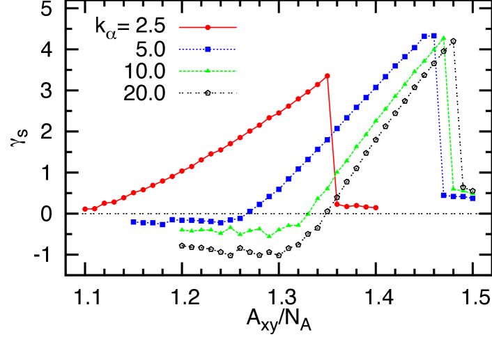
Figure 1: Area dependence of surface tension $\gamma_{\rm s}$ for the explicit solvent meshless membrane model is plotted for $k_{\alpha}=2.5,5,10,$ and 20 with $\epsilon=4$.

First, a planar fluctuating membrane is simulated with the particle numbers $N_{\mathcal{A}}=1600$ (and $N=48\ 000$ or $64\ 000$). For various membrane projected areas $A_{xy}=L_{x}L_{y}$, the surface tension

$$\gamma_{\rm s}=\langle P_{zz}-(P_{xx}+P_{yy})/2\rangle L_{z}$$ (11)

is investigated. Here, $P_{\mu\nu}$ is the pressure tensor given by

$$P_{\mu\nu}=\sum_{i=1}^{N}\left(mv_{i}^{\mu}v_{i}^{\nu}-\mu_{i}\frac{\partial U}{\partial\nu_{i}}\right)\Big{/}V,$$ (12)

where $\{\mu,\nu\}\in\{x,y,z\}$, $\bm{v}_{i}=(v_{i}^{x},v_{i}^{y},v_{i}^{z})$, and the sum is taken over all the particles including the solvent component. In calculating $P_{\mu\nu}$, the periodic image $\mu_{i}+nL_{\mu}$ nearest to the other interacting particles is employed, when the potential interaction crosses one of the periodic boundaries.

Figure 1 shows the dependence of $\gamma_{\rm s}$ on the projected membrane area $A_{xy}$ for $k_{\alpha}=2.5,5,10$, and 20, with $\epsilon=4$. For $\gamma_{\rm s}\simeq 0$, the intrinsic area $A$ is larger than $A_{xy}$ due to the membrane undulations; buckling of the membrane occurs for $A<A_{xy}$ (the flat region at $\gamma_{\rm s}<0$ in Fig. 1). Noguchi (2011) For tension-less membranes with $N_{\mathcal{A}}=1600$, the projected area $A^{0}_{xy}$ is given by $A_{xy}^{0}=a^{0}_{xy}N_{\mathcal{A}}$ with $a_{xy}^{0}=1.1,\ 1.27,\ 1.33,\ 1.35$ for $k_{\alpha}=2.5,\ 5,\ 10,\ 20$, respectively. The projected membrane area increases with increasing $k_{\alpha}$, because both membrane bending fluctuations and protrusions are suppressed at larger $k_{\alpha}$.

Figure 2: Dependence of the bending rigidity $\kappa$ on $k_{\alpha}$ is plotted for $\epsilon=4$, estimated with the use of a tension-less planar membrane at $N_{\mathcal{A}}=1600$ through Eq. (13). As shown in the inset, the height spectrum of the membrane exhibits a $q^{-4}$ spectrum.

Figure 3: $\epsilon$ dependence of the line tension $\Gamma$ of explicit-solvent meshless-membrane model, calculated for $k_{\alpha}=5$ and $10$ with the use of Eq. (14).

Figure 2 shows the bending rigidity $\kappa$ as a function of $k_{\alpha}$. Here, the bending rigidity is estimated from the height spectrum Helfrich (1973)

$$\langle|h(q)|^{2}\rangle=\frac{k_{\rm B}T}{\gamma_{\rm s}q^{2}+\kappa q^{4}}.$$ (13)

of the tension-less membrane ($\gamma_{\rm s}=0$). In calculating $\langle|h(q)|^{2}\rangle$, the raw positional data of the membrane particles ($\bm{r}_{i},\ i\in\mathcal{A}$) is employed. Noguchi and Gompper (2006a); Shiba and Noguchi (2011) Because of the slow dynamics of long-wavelength height fluctuations, it becomes more time-consuming to obtain precise data than for the implicit-solvent model. Noguchi and Gompper (2006a); Shiba and Noguchi (2011) Therefore, $\langle|h(q)|^{2}\rangle$ is measured using 16 independent runs for each $k_{\alpha}$, and the averaged spectrum is then fitted to Eq. (13) in the range $q<1.2\sigma^{-1}$. As in the implicit model, the bending rigidity is found to be proportional to $k_{\alpha}$, which demonstrates the controllability of $\kappa$ in our model.

In Fig. 3, the $\epsilon$ dependence of the line tension $\Gamma$ is displayed for $k_{\alpha}=5$ and 10 for a membrane strip with two edges with lengths equal to $L_{x}$ with $N_{\mathcal{A}}=1600$. Here, $\Gamma$ is determined via the relation Shiba and Noguchi (2011)

$$\Gamma=\langle(P_{yy}+P_{zz})/2-P_{xx}\rangle L_{y}L_{z}/2.$$ (14)

At a small $\epsilon$, $\Gamma$ is proportional to $\epsilon$ and almost independent of $k_{\alpha}$, similarly to the implicit-solvent meshless membrane model Noguchi and Gompper (2006a). While $\Gamma$ increases linearly up to $\epsilon=8$ for $k_{\alpha}=10$, it levels off and saturates at $\epsilon=4$ for $k_{\alpha}=5$. When $\epsilon$ exceeds the value where $\Gamma$ saturates — a value which becomes larger for larger $k_{\alpha}$ — the membrane particles prefer to reside at the edges, because the curvature force is not strong enough to avoid aggregation due to the stronger attractive forces.

For our simulations of membrane ensembles in shear flow, we choose the model parameters $k_{\alpha}=5$ and $\epsilon=4$, where the membrane has bending rigidity $\kappa/k_{B}T=11\pm 1$. With the estimated values for the line tension $\Gamma\sigma/k_{\rm B}T=4.2\pm 0.2$, the relaxation time scale of structural transitions can be characterized by

$$\tau=\frac{\eta R_{c}^{3}}{\kappa},$$ (15)

where $\eta$ is the solvent viscosity, and $R_{c}$ is the critical radius of a flat disk. Assuming a flat disk with radius $R$ and a vesicle with the same membrane area, we obtain the corresponding elastic free energies $\mathcal{F}_{d}=2\pi R\Gamma$ and $\mathcal{F}_{s}=8\pi(\kappa+\bar{\kappa}/2)\simeq 4\pi\kappa$; thus, a disk exhibits transition to closed vesicle shape if the radius is around

$$R_{c}=2\kappa/\Gamma\sim(5.3\pm 0.5)\sigma.$$ (16)

With the solvent viscosity $\eta=(2.1\pm 0.1)\times m(\sigma t_{0})^{-1}$ obtained from a solvent-only simulation, an estimation of the relaxation time yields $\tau=28.4t_{0}$. In the following, the time will be measured in unit of $\tau$. Since the membrane thickness, typically around 5nm for non-ionic surfactants like polyethylene-glycol-ethers C_nE_m, corresponds to the size $\sigma$ of the membrane particles in our simulation, $\tau$ is equivalent to about $0.36\mu$s (with the viscosity of water at 300K, $\eta_{\rm w}\simeq 0.8{\rm mPa}\cdot{\rm s}$).

IV Structure Formation with and without Shear Flow

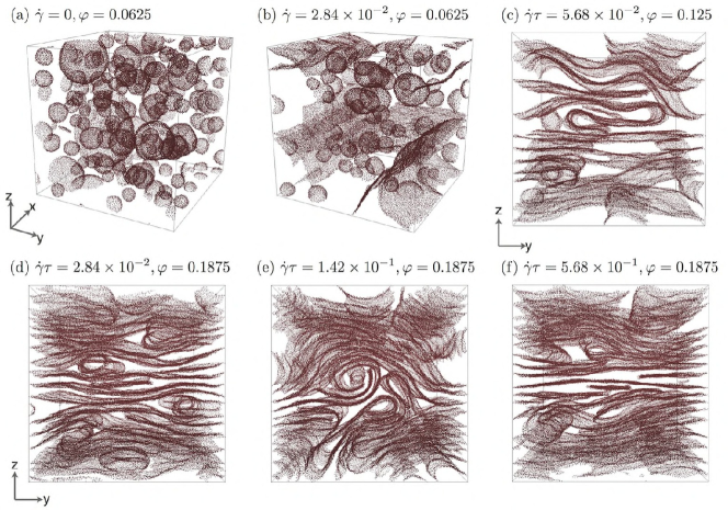
Figure 4: Snapshots of the configuration of membrane particles for $\varphi=0.0625$ (a) without shear ($\dot{\gamma}=0$) and (b) under shear flow with shear rate $\dot{\gamma}\tau=0.0284$, and (c) for $\varphi=0.125$ with $\dot{\gamma}\tau=0.0568$. Snapshots for $\varphi=0.1875$ under shear flow are shown with shear rates (d) $\dot{\gamma}\tau=0.0284$, (e) $\dot{\gamma}\tau=0.142$, and (f) $\dot{\gamma}\tau=0.568$. In (b)-(f), the (average) imposed flow velocity is ${\bf v}=\dot{\gamma}z{\bf e}_{x}$. Solvent particles are not displayed.

We now employ the meshless-membrane model with explicit solvent to study structure formation in surfactant-water mixtures, both with and without shear flow. In all simulations, the total particle number is fixed at $N=N_{\mathcal{A}}+N_{\mathcal{B}}=960\ 000$, and thus, the system size is a cubic box with side length $L=114.47\sigma$. Simulations are performed for various membrane volume fraction $\varphi=N_{\mathcal{A}}/N$, with $\varphi=0.0625$, $0.125$, $0.1875$, $0.25$, and $0.3125$. The dynamical evolution is integrated over a total time interval of $1.2\times 10^{7}$ MD steps, corresponding to $2.11\times 10^{3}\tau$. All the particles of both species are initially distributed randomly in the simulation box. Averages are calculated over the last $2\times 10^{6}$ steps, where the system is assumed to have reached a stationary state. After briefly explaining the structures obtained by equilibrium simulations without shear in Sec. IV.1, we present results for the structure formation in a system under linear shear flow in Secs. IV.2 and IV.3.

IV.1 Mesophases in Thermal Equilibrium

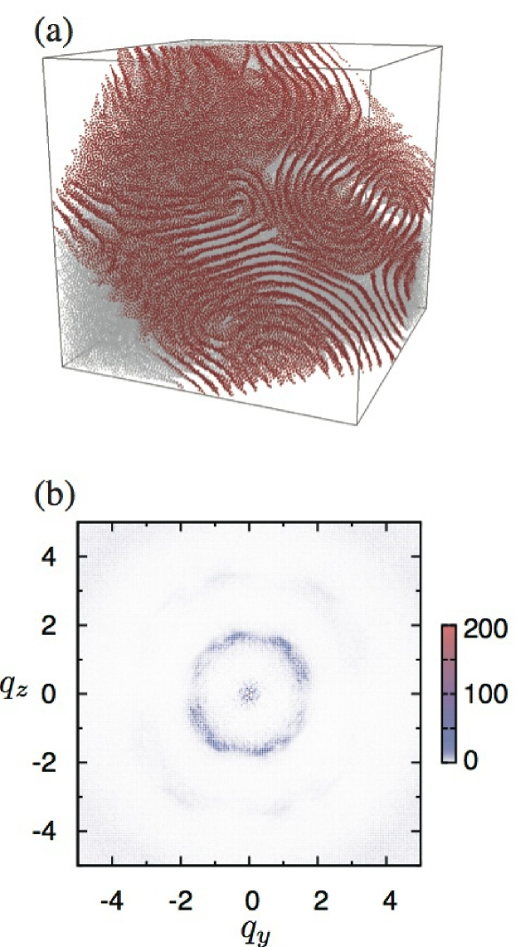
Figure 5: (a) Snapshot of the configuration of membrane particles for $\varphi=0.3125$ without shear flow ($\dot{\gamma}=0$). To facilitate visualization, only a thin planar slice is displayed. Solvent particles are not shown. (b) Structure factor $S_{\mathcal{A}}[\bm{q}=(0,q_{y},q_{z})]$ for $\varphi=0.3125$ at $\dot{\gamma}=0$.

At a low membrane volume fraction $\varphi=0.0625$, membrane particles self-assemble into vesicles, each of which is composed of around $100$ membrane particles (see Fig. 4(a)). This result is consistent with Eq. (16), which predicts the critical particle number of a vesicle to be $N_{c}=\pi R_{c}^{2}/a^{0}\simeq 75$. At a higher membrane volume fraction $\varphi=0.125\ (N_{\mathcal{A}}=120\ 000)$, the membrane surfaces is found to percolate through the whole system via the periodic boundaries. This behavior is not unexpected, because each disk with radius $R_{c}$ covers a region of volume $v_{c}=(2R_{c})^{3}$ by rotational diffusion, and therefore these disks should overlap and merge when more than $n_{c}\sim V/v_{c}=1200$ vesicles are present, which exceeds the number of vesicles with critical size ($N_{\mathcal{A}}/N_{c}$).

For $\varphi=0.25$ and 0.3125, periodic lamellar states are formed owing to the repulsive interactions between the membranes, as shown in Fig. 5(a). The membranes are curved to fill up space with random orientations. In thermal equilibrium, these lamellar layers would probably have a unique orientation throughout the system; this well-ordered state is difficult to reach in simulations because the structural relaxation time well exceeds the accessible simulation time scale. The 3D structure factor of the membrane density is calculated as

$$S_{\mathcal{A}}(\bm{q})=\int d\bm{r}\ e^{i\bm{q}\cdot\bm{r}}\langle\delta\hat{n}_{\mathcal{A}}(\bm{r})\delta\hat{n}_{\mathcal{A}}(\bm{0})\rangle,$$ (17)

where $\delta\hat{n}_{\mathcal{A}}(\bm{r})=\sum_{i\in\mathcal{A}}\sigma^{3}\delta(\bm{r}-\bm{r}_{i})-\phi$ is the local deviation of the membrane particle density from its average. Figure 5(b) shows $S_{\mathcal{A}}(\bm{q})$ for $\varphi=0.3125$. The scattering intensity is spherically symmetric, as demonstrated by a two-dimensional (2D) color-map for $q_{z}=0$. Peaks arising from the inter-lamellar distance are observed at $|\bm{q}|=q_{1}=1.74\sigma^{-1}$ and $q_{2}=3.49\sigma^{-1}=2q_{1}$ with heights 9.8 and 0.78, respectively. The former corresponds to length of $L=2\pi/q_{1}=3.61\sigma$, which provides a precise estimate of the interlayer distance.

IV.2 Dynamic Phase Diagram under Shear Flow

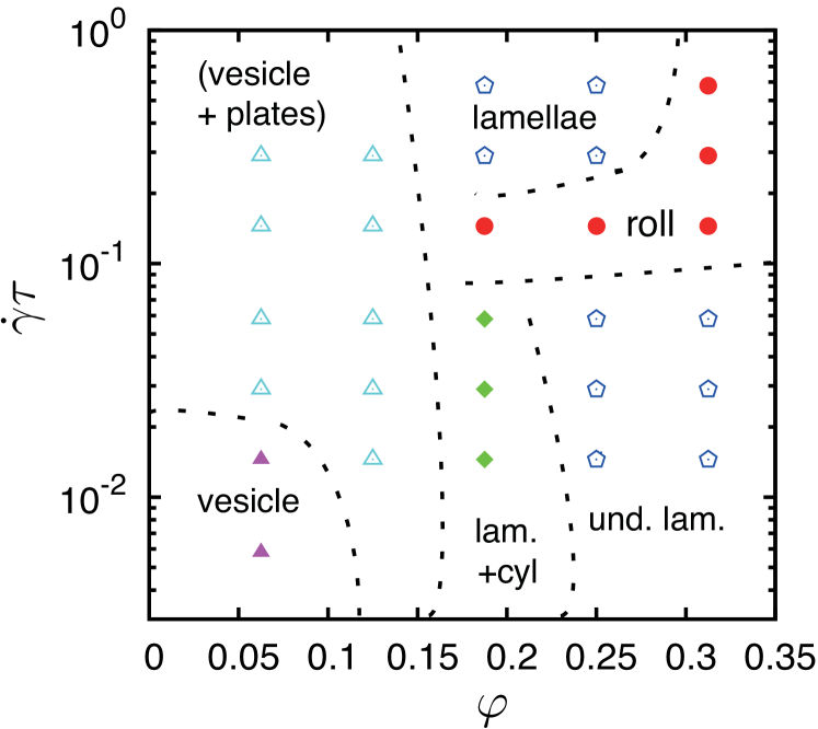
Figure 6: Dynamic phase diagram of the explicit-solvent meshless-membrane model as a function of the volume fraction $\varphi$ of the membrane component and the shear rate $\dot{\gamma}$. The parameters are $k_{\alpha}=5$, $\epsilon=4$, $\phi=0.64\sigma^{-3}$, and $N=960,000$. The dashed lines are guides to the eye.

In shear flow, the vesicle and lamellar states depend on the concentration $\varphi$ and the shear rate $\dot{\gamma}$, as displayed in Fig. 6. At $\varphi=0.0625$, assemblies of uni-lamellar vesicles are observed for $\dot{\gamma}\tau<0.02$. At a higher shear rate, the membrane particles tend to assemble into plate-like membrane disks, which then align parallel to the shear flow direction, as demonstrated by the comparison of snapshots in Figs. 4 (a) and (b). At $\varphi=0.125$, lamellar layers with non-uniform lamellar distances are observed for $\dot{\gamma}\tau<0.06$, as shown in Fig. 4(c). There is a larger variety of phases at $\varphi=0.1875$; at low shear rates $\dot{\gamma}\tau<0.1$, the system is a mixture of lamellae and cylinders as shown in Fig. 4(d); at $\dot{\gamma}\tau=0.142$, the lamellae are rolled up collectively, see Fig. 4(e); finally, at large shear rates $\dot{\gamma}\tau\gtrsim 0.3$, the system exhibits a reentrant lamellar state, as shown in Fig. 4(f).

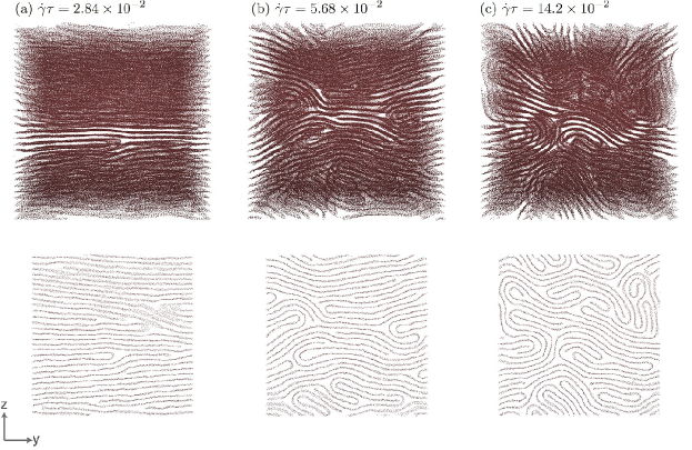
Figure 7: Snapshots membrane conformations for volume fraction $\varphi=0.3125$, with shear rates (a) $\dot{\gamma}\tau=0.0284$, (b) $\dot{\gamma}\tau=0.0568$, and (c) $\dot{\gamma}\tau=0.142$. Views from the flow ($x$) direction are shown in the upper panels. Corresponding cross-sectional views (with $-3.0\sigma<x<3.0\sigma$) are shown in the lower panels.

At higher $\varphi$, the lamellar states align perpendicularly to the shear-gradient ($z$) direction in the regime of low shear rates ($\dot{\gamma}\tau<0.1$). At larger $\dot{\gamma}$, they exhibit an instability to a rolled-up shape whose axis is parallel to the flow direction, which will be investigated in more detail in Sec. IV.3 below. At $\varphi=0.25$, there is again a reentrant behavior of lamellar states, i.e. nearly planar aligned layers appear at large shear rates $\dot{\gamma}\tau\geq 0.284$. Note that experimental phase diagrams often exhibit reentrant behaviors Roux et al. (1993); Diat et al. (1993) with increase in the shear rate at a certain membrane volume fraction; the mixture changes from lamellar state to onion state, and then after going through the coexistence region it enters again into an oriented lamellar state again. Although the onion state with densely packed MLVs has not been obtained in our simulations, the reentrant behavior is qualitatively consistency with the experimental observations.

IV.3 Rolled-up Lamellar Structures

IV.3.1 Structure Analysis

Snapshots of membrane conformations are shown in Fig. 7 for $\varphi=0.3125$ at various shear rates $\dot{\gamma}\tau=0.0284$, $0.0568$, and $0.142$. In all simulations for $\varphi\geq 0.125$, the membranes are completely aligned with the flow direction. Thus, as shown in the bottom panel of Fig. 7, the membrane configurations can be visualized by cross-sectional slices perpendicular to the flow direction. Figure 7 demonstrates the transition from the lamellar state to the rolled-up state, which is stable in the region $\varphi\gtrsim 0.175$ and $\dot{\gamma}\tau\gtrsim 0.1$ in the phase diagram of Fig. 6.

The structural changes accompanying this instability can be characterized by the average orientation and the mean-square local curvature of the membrane. The normal unit vector $\bm{n}$ is calculated from the first-order moving least-squares (MLS) method Noguchi and Gompper (2006a); Belytschko et al. (1996); Lancaster and Salkaskas (1981) applied to the configurations of membrane particles. Using a weighted gyration tensor $a_{\alpha\beta}=\sum_{j}(\alpha_{j}^{\prime}-\alpha_{G}^{\prime})(\beta_{j}^{\prime}-\beta_{G}^{\prime})w_{\rm cv}(r_{ij})$, where $\alpha,\ \beta\in\{x,y,z\}$, $\bm{n}$ is obtained as an eigenvector corresponding to the minimum eigenvalue of $a_{\alpha\beta}$, which together with the other two eigenvectors $\bm{e}_{1}$ and $\bm{e}_{2}$ constitutes an orthonormal basis. Here, the cut-off function $w_{\rm cv}(r_{ij})$ in Eq. (8) is employed with the same cut-off lengths $r_{cc}^{\prime}=3.2\sigma$. As a quantitative measure for the undulation instability, we employ the orientational order parameter

$$S_{z}=[2({\bm{n}}\cdot\hat{\bm{e}}_{z})^{2}-1]=\cos(2\theta)$$ (18)

with the normalization for the two-dimensional order of cylindrical and planar symmetry.

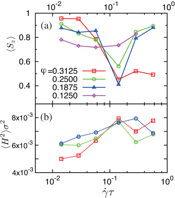
Figure 8: (a) Membrane orientational order parameter $\langle S_{z}\rangle$ in Eq. (18) for $\varphi=0.125$, $0.1875$, $0.25$, and $0.3125$, and (b) the mean-square local curvature $\langle H^{2}\rangle$ for $\varphi=0.1875$, $0.25$, and $0.3125$, both as function of the shear rate $\dot{\gamma}\tau$.

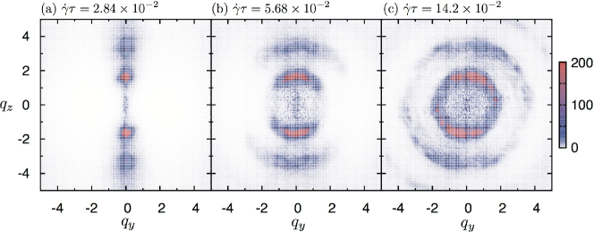
Figure 9: Color maps of the structure factor $S_{\mathcal{A}}(0,q_{y},q_{z})$ for volume fraction $\varphi=0.3125$ and shear rates (a) $\dot{\gamma}\tau=0.0284$, (b) $\dot{\gamma}\tau=0.0568$, and (c) $\dot{\gamma}\tau=0.142$. Since the structure is uniform in the flow ($x$) direction, only data for $q_{x}=0$ are shown.

The instability can also be characterized by calculating the mean-square curvature. The second-order MLS method Noguchi and Gompper (2006a) provides an estimate of the membrane curvature from the particle configurations in the following way. For each particle $i$, we perform a rotational transformation into the principal coordinate system of the gyration tensor of the neighbor particles $j$ around $i$’s weighted center of mass $\bm{r}_{G}$ by

$$\left(\begin{array}[]{c}X_{j}\\ Y_{j}\\ Z_{j}\end{array}\right)=\left(\begin{array}[]{c}\bm{e}_{1}\\ \bm{e}_{2}\\ \bm{n}\\ \end{array}\right)(\bm{r}_{j}-\bm{r}_{G})^{T},$$ (19)

and then employ the parabolic fit function

$$\begin{array}[]{rl}\Lambda_{2}(\bm{r}_{i})&=\frac{1}{w_{0}}\sum_{j}\left(z_{0}+h_{x}X_{j}+h_{y}Y_{j}+\frac{1}{2}h_{xx}X_{j}^{2}\right.\\ &+\left.\frac{1}{2}h_{yy}Y_{j}^{2}+h_{xy}X_{j}Y_{j}-Z_{j}\right)^{2}w_{\rm cv}(r_{ij}),\end{array}$$ (20)

where the coefficients of the Taylor expansion $z_{0},\ h_{x},\ h_{y},\ h_{xx},\ h_{yy}$ and $h_{xy}$ are fitting parameters. Noguchi and Gompper (2006a) By a least-squares fit, the estimated value of the mean curvature $H=(C_{1}+C_{2})/2$ for particle $i$ is then obtained as

$$H=\frac{(1+h_{x}^{2})h_{yy}+(1+h_{y}^{2})h_{xx}-2h_{x}h_{y}h_{xy}}{2(1+h_{x}^{2}+h_{y}^{2})^{3/2}}.$$ (21)

Figure 8 displays the results for the spatial average $\langle S_{z}\rangle$ of the 2D orientational order parameter and for the mean-square local curvature $\langle H^{2}\rangle$. When the membranes are aligned with the $x-y$ plane orthogonal to the shear-gradient direction, $S_{z}$ becomes unity. As the membranes roll up, $S_{z}$ decreases. Here, $\langle S_{z}\rangle=0$ for perfectly cylindrical state (where $({\bm{n}}\cdot\hat{\bm{e}}_{x})^{2}=0$ and $({\bm{n}}\cdot\hat{\bm{e}}_{y})^{2}=({\bm{n}}\cdot\hat{\bm{e}}_{z})^{2}=1/2$ ), and $\langle S_{z}\rangle=-1$ for a perfectly flat lamellar layers perpendicular to the vorticity ($y$) direction (where $({\bm{n}}\cdot\hat{\bm{e}}_{z})^{2}=0$). For all $\varphi\geq 0.1875$, the values of $\langle S_{z}\rangle$ and $\langle H^{2}\rangle$ provide evidence for rolled-up structures at $\dot{\gamma}\tau=0.142$. For $\varphi=0.1875$ and 0.25, $\langle S_{z}\rangle$ increases again at $\dot{\gamma}\tau=0.284$, indicating reentrant alignment of the membranes in a lamellar stack. However, for $\varphi=0.3125$, $\langle S_{z}\rangle$ remains small (and $\langle H^{2}\rangle$ large), which implies that rolled-up structures exist also at $\dot{\gamma}\tau=0.284$. Thus, the evolution of rolled-up conformations is the most pronounced at the highest membrane volume fraction $\varphi=0.3125$.

In Fig. 9, results for the structure factor $S_{\mathcal{A}}(\bm{q})$ at $q_{x}=0$ are shown for the same set of data as in Fig. 7. Due to the nearly complete alignment of membranes in the flow ($x$) direction, all the structural features are reflected in $S_{\mathcal{A}}(\bm{q})$ in the $q_{y}-q_{z}$ wave-vector plane. Since lamellar layers are nearly planar at the low shear rate $\dot{\gamma}\tau=0.0284$, a sharp peak is observed around $(q_{y},q_{z})=(2\pi q_{1},0)$. Because of the undulation instability, the pattern becomes more circular at higher $\dot{\gamma}$.

In the small-angle neutron Nettesheim et al. (2003) and X-ray Ito et al. (2011) scattering experiments, the scattering beams can be injected from two directions, either radial or tangential to the shear cell, which correspond to shear-gradient and flow directions, respectively. After the shear flow is applied, after a while a Bragg peak of the radial beam develops in the vorticity direction, while the scattering pattern becomes isotropic for the tangential beam. This suggests 2D-isotropic undulations of the lamellar structure perpendicular to the flow direction. Later in time, the radial beam is scattered isotropically in the tangential direction, indicating the formation of onion structures. The structure factor $S(\bm{q})$ in our simulation (Fig. 9(c)), agrees well with $S(\bm{q})$ of this transient states in these scatting experiments. Measurements of solvent diffusion in a Rheo-NMR experiment of a non-ionic surfactant system Medronho et al. (2008) show a diffusion anisotropy in the direction of shear flow in the intermediate state. These experimental results suggest that the membranes are aligned in the direction of shear flow in the intermediate state of the lamellae-to-onion transition, although more detailed information on the structural membrane arrangement could not be obtained. The rolled-up lamellar structures observed in our simulations match the experimental evidence, so that they are a good candidate for the intermediate states.

IV.3.2 Temporal Evolution of Membrane Structures

In simulations of a large system, even if extended over a long time interval, the resultant structure often exhibits dependence on the initial conditions – owing to the slow processes involved in the dynamics. Therefore, we compare here the time evolution at $\varphi=0.3125$ starting from both, a lamellar state and a random distribution of membrane particles (the latter corresponding to the simulations described in the previous subsections). For an initial lamellar state, the final configuration of a simulation run with $1.2\times 10^{7}$ MD steps at a small shear rate $\dot{\gamma}\tau=0.0284$ (see Fig. 7(a)), is employed.

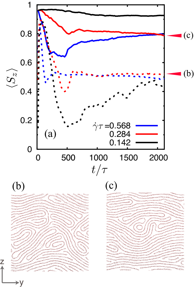
Figure 10: Comparison of structure formation from a random initial configuration and from a lamellar state at $\varphi=0.3125$. (a) Time evolution of the orientational order parameter $\langle S_{z}\rangle$. The dotted and solid lines show the data starting from the random and lamellar initial states, respectively. Blue, red, and black lines represent the shear rates $\dot{\gamma}\tau=0.568$, $0.284$, and $0.142$, respectively. Snapshots of the final configurations for $\dot{\gamma}\tau=0.284$ at $t=2.11\times 10^{3}\tau$, as they have developed from (b) the random and (c) the lamellar initial states, are also shown.

In Fig. 10(a), the orientation order parameter $\langle S_{z}\rangle$ for both initial conditions are shown for $\dot{\gamma}\tau=0.568$, $0.284$, and $0.142$. For the case of a random initial distribution, small disks merge into randomly oriented surfaces, which then align in the shear flow to become a nearly perfect lamellar stack with some defects. Afterwards, lamellae roll up into slightly larger rolls. During rolling up, $\langle S_{z}\rangle$ exhibits an overshoot (see Fig. 10(c)), and finally approaches a constant as the structure relaxes into a (meta)stable state. The overshoot amplitude depends on initial states and random noises.

Figs. 10(b) and (c) show the membrane conformations after an elapsed time of $t=2.11\times 10^{3}\tau$ (for $\dot{\gamma}\tau=0.284$) for the two types of initial conditions, and explain the origin of the substantially different values of the order parameter $\langle S_{z}\rangle$ in Fig. 10(a). When the random state is taken as initial condition, rolled-up structures are considerably more pronounced; this may be traced back to the presence of defects in the lamellar structure which forms at short times $t/\tau\simeq 100$.

For the case of a lamellar initial configuration, the undulation instability becomes more conspicuous when the applied shear flow is stronger. Moreover, while strong undulations are observed at low $\dot{\gamma}$ with the random initial configuration, less undulations take place with the lamellar initial configuration, as indicated by $\langle S_{z}\rangle\sim 1$. Thus, the initial conditions play an important role in the selection of the transition path and structure formation. It may depend not only on the shear rate and relaxation time but also on the distribution of structural defects in the lamellar layers. Thus, more systematic studies are required in the future to clarify the hysteresis of these systems.

V Summary

In this paper, we have constructed an explicit-solvent meshless-membrane model for surfactant-water mixtures. The model reproduces properties of an earlier implicit-solvent meshless membrane model, where membrane bending rigidity and line tension can be independently controlled to a large extent. The model enables large-scale simulations of structural changes, where dynamical effects of hydrodynamic interactions have to be taken into account. At present, such a large simulation with as many as one-million particles can be realized by parallelized molecular dynamics simulation methods.

Our main results concern the effects of shear flow on the structure formation of membrane ensembles. Various structures including vesicles, lamellae, and multi-lamellar states with nearly cylindrical symmetry have been found, most of which are qualitatively consistent with experimental observations of non-ionic surfactant membranes under shear flow. Especially, a cylindrical instability of multi-lamellar membrane is predicted to occur perpendicularly to the flow direction. The corresponding scattering patterns are in qualitatively agreement with the results of small angle neutron (and X-ray) scattering experiments under shear deformation. The rolled-up lamellae are a good candidate for the intermediate structures on the way to the onion state, which are observed in the experiments.

Our simulations do not reproduce onion formation, which is ubiquitously observed in experiments on $\mu$m length scales. We speculate that it is due to the limited system size, which can be overcome by larger-scale calculations in the future. On the other hand, in the experiments, strains larger than $\dot{\gamma}t\gtrsim 10^{4}$ are necessary to reach the onion state, which indicates that very long simulation runs are required to obtain these states.

The control of the physical parameters including the line tension $\Gamma$, the bending rigidity $\kappa$, and the Gaussian modulus $\bar{\kappa}$ is another challenge. While $\Gamma$ and $\kappa$ are easily controlled in our model, $\bar{\kappa}$ is more difficult. The Gaussian modulus $\bar{\kappa}$ might also play an important role in the structure formation, because it is directly related to topological changes happening on the way of onion formation. Hu et al. (2012)

Appendix A Solvent-Mediated Forces at Higher Solvent Density

In the present simulation model, solvent particles have a similar size as membrane particles. Here, we discuss the finite-size effects of the solvent particles, if much higher solvent densities are used than in the present study. When the solvent particles are densely packed, the system approaches a crystallization transition, and local crystalline order emerges to bring about interactions between closely spaced lamellar layers.

As an example, we study the explicit-solvent meshless-membrane model for higher number density (denoted system $(\mathcal{S}2$), where $\phi=(\sigma_{\mathcal{A}}^{3}N_{\mathcal{A}}+\sigma_{\mathcal{B}}^{3}N_{\mathcal{B}})/V=0.72$ with the total particle number $N=N_{\mathcal{A}}+N_{\mathcal{B}}=480\ 000$). The particle radii of the two components are chosen such as $\sigma_{\mathcal{B}}=1.2\sigma_{\mathcal{A}}$, where $\sigma_{\mathcal{A}}$ and $\sigma_{\mathcal{B}}$ denote the radii of membrane and solvent components, respectively. The cut-off lengths of the interactions are set to $r_{c}^{\rm rep}=2.7\sigma_{\mathcal{A}},r_{\rm ga}=1.5\sigma_{\mathcal{A}},\ r_{\rm cc}=3.0\sigma_{\mathcal{A}}$, respectively. The repulsive inverse twelfth-power potential exhibits melting transition around the volume fraction around 0.43 (corresponding to $\phi\simeq 0.8$ in our definition). Hoover et al. (1970) Thus, our density $\phi=0.72$ is close to the crystallization line.

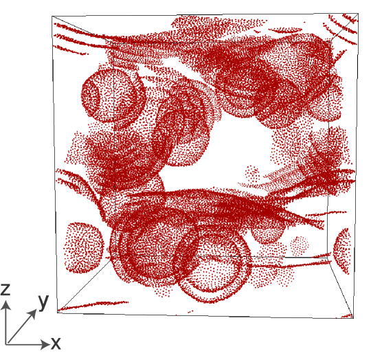
Figure 11: Snapshot of the MLV state due to the solvent-mediated attractive interactions for the system $\mathcal{S}2$ at $\phi=0.72$, $\varphi=0.06$ and $N=480,000$ with different size ratio $\sigma_{\mathcal{B}}/\sigma_{\mathcal{A}}=1.2$, for shear rate $\dot{\gamma}\tau=0.0142$.

As an example, Fig. 11 shows a snapshot for membrane volume fraction $\varphi=N_{\mathcal{A}}\sigma_{\mathcal{A}}^{3}/(N_{\mathcal{A}}\sigma_{\mathcal{A}}^{3}+N_{\mathcal{B}}\sigma_{\mathcal{B}}^{3})=0.06$ for a shear rate $\dot{\gamma}\tau=0.0142$. After an initial relaxation from a random configuration of the membrane particles, the membrane layers assemble into stacks, and then form MLVs after gathering a certain amount of the membrane patches. In the snapshot, the layers are stacked with distances $d\simeq 3.0\sigma_{\mathcal{B}}$, which seems to arise from the discreteness of the interstitial solvent particles – here it should be noted that interlayer distance cannot be smaller than $d\simeq 2.0\sigma_{\mathcal{B}}$ because it is inside the range of $U_{\rm rep}$ and $U_{\alpha}$, which both act repulsively.

Figure 12: Equilibrium lamellar distance $d_{\rm lam}$ versus initial lamellar distance $d_{\rm ini}$ between a tension-less planar membrane and two (smaller) membrane discs. For the systems $\mathcal{S}1$ and $\mathcal{S}2$, lengths are represented in units of $\sigma$ and $\sigma_{\mathcal{A}}$, respectively. The dotted line indicates the line $d_{\rm ini}=d_{\rm lam}$.

To avoid this solvent-mediated force, a longer cut-off range of the repulsive forces and a lower density are employed in the simulation described in the main text (denoted system ($\mathcal{S}1$)). To demonstrate the difference between the systems $\mathcal{S}1$ and $\mathcal{S}2$, we simulate three lamellar layers in the following way. A periodic simulation box with lengths $L_{x}=L_{y}=\sqrt{A_{xy}^{0}}/\sigma_{\mathcal{A}}$, $L_{z}=V/(L_{x}L_{y})$ is set up so that a tension-less membrane (with particle number $N_{\mathcal{A}0})=1600$ is put along the $xy$-plane. Here, the projected areas are set to $A_{xy}^{0}=1.267N_{\mathcal{A}0}$ for $\mathcal{S}1$ and $A_{xy}^{0}=1.335N_{\mathcal{A}0}$ for $\mathcal{S}2$, respectively. With various interlayer distance $d_{\rm ini}$, circular membrane disks with particle number $N_{\mathcal{A}1}=N_{\mathcal{A}2}=400$ are put on both sides of the membrane. Solvent particles are then inserted to fill up the system; they are relaxed for fixed membrane configuration for $10^{5}$ MD steps. Afterward, a simulation of the full system is performed for $1.5\times 10^{6}$ MD steps to obtain an equilibrium interlayer distance $d_{\rm lam}$. As shown in Fig. 12, while the interlayer distance increases with time in the $\mathcal{S}1$ case, there are stable lamellar distances around $d_{\rm lam}=3.5\sigma_{\mathcal{A}}$ and $4.7\sigma_{\mathcal{A}}$ in the $\mathcal{S}2$ case with higher solvent density, which correspond to $3\sigma_{\mathcal{B}}$ and $4\sigma_{\mathcal{B}}$, respectively. Thus, in $\mathcal{S}2$, the effective attractive potentials lead to the stable multi-lamellar layers due to the attractive interactions.

Appendix B Numerics and Parallelization

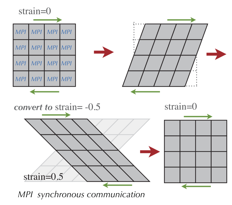
Figure 13: Schematic picture in two dimensions for the implementation of Lees-Edwards boundary conditions in a program parallelized with MPI communication.

Numerical simulations have been carried out on massively parallel supercomputers. On 256 CPUs of Intel Xeon X5570 (2.93GHz) in SGI Altix ICE 8400EX at ISSP, it costs 72 hours to perform a run of $1.2\times 10^{7}$ simulation steps for $\varphi=0.3125$ and $N=960,000$. Here, about 10% of the total time is for the force calculation of $U_{\rm rep}$, 30% for $U_{\alpha}$, around 20% for the construction of the buffer, and 20% for the communication between the MPI processes. The system is divided into cubic (or rectangular) boxes, each of which is calculated by one MPI process. We also parallelize calculations of each process with the use of OpenMP by performing calculations of different far away pairs at once on different threads. The code is optimized to achieve 15% performance compared with the theoretical limit on X5570 processors.

Each process has separate cell lists and neighbor lists for solvent and membrane particles. To apply shear, we employ a simultaneous affine deformation of the total system, each MPI process box, and each cell for neighbor search, so that a square is transformed into a parallelogram shape consistent with the shear deformation, as illustrated in Fig. 13. When the strain reaches 0.5, these parallelograms are reflected to make the strain -0.5, see Fig. 13, which basically requires an all-to-all communication of all the position and velocity data.