Femtoscopic scales in $p+p$ and $p+$Pb collisions in view of the uncertainty principle

Abstract

A method for quantum corrections of Hanbury-Brown/Twiss (HBT) interferometric radii produced by semi-classical event generators is proposed. These corrections account for the basic indistinguishability and mutual coherence of closely located emitters caused by the uncertainty principle. A detailed analysis is presented for pion interferometry in $p+p$ collisions at LHC energy ($\sqrt{s}=7$ TeV). A prediction is also presented of pion interferometric radii for $p+$Pb collisions at $\sqrt{s}=5.02$ TeV. The hydrodynamic/hydrokinetic model with UrQMD cascade as ’afterburner’ is utilized for this aim. It is found that quantum corrections to the interferometry radii improve significantly the event generator results which typically overestimate the experimental radii of small systems. A successful description of the interferometry structure of $p+p$ collisions within the corrected hydrodynamic model requires the study of the problem of thermalization mechanism, still a fundamental issue for ultrarelativistic $A+A$ collisions, also for high multiplicity $p+p$ and $p+$Pb events.

PACS: 24.10.Nz, 24.10.Pa, 25.75.-q, 25.75.Gz, 25.75.Ld.

Keywords: correlation femtoscopy, HBT radii, proton-proton collisions, proton-nucleus collisions, LHC, uncertainty principle, coherence

I Introduction

The quantum-statistical enhancement of the pairs of identical pions produced with close momenta was observed first in $\bar{p}+p$ collisions in 1959 Gold . It took more than a decade to develop the method of pion interferometry based on the discovered phenomenon. This was done at the beginning of the 1970s by Kopylov and Podgoretsky Kopylov . Their theoretical analysis assumed the radiating source as consisting of independent incoherent emitters. In fact, such a representation is used for a long time for the analysis of the space-time structure of particle sources created in $\bar{p}+p$, $p+p$, $e^{+}+e^{-}$ and $A+A$ collisions. The concept of independent emitters was applied to a further development of the interferometric method, in particular, to account for momentum-position correlations of the emitted particles  Pratt ; MakSin ; Sinyuk ; Hama that, in turn, has resulted in a general interpretation of the measured radii as the homogeneity lengths in the Wigner functions Sin ; AkkSin ; SinAkkKarp . This concept is important for a study of $A+A$ collision processes within the hydrodynamic approach. Also a detailed analysis of the particle final state (Coulomb) interactions brings the significant contribution to the traditional method of correlation femtoscopy FSI ; baym .

In a recent paper SinShap the correlation analysis is taken beyond the model of independent particle emitters. It is found that the uncertainty principle leads to (partial) indistinguishability of closely located emitters that fundamentally impedes their full independence and incoherence. The partial coherence of emitted particles is because of the quantum nature of particle emission and happens even if there is no specific mechanism to produce a coherent component of the source radiation. This effect leads to a reduction of the interferometry radii and suppression of the Bose-Einstein correlation functions. The effect is significant only for small sources with typical sizes less than 2 fm. We shall apply this approach SinShap to the analysis of data in $p+p$ collisions at the LHC energy of $\sqrt{s}=7$ TeV, where the measured interferometry radii are just within the above scale. A simple estimate will be done also for $p+$Pb, where the radii are larger and such corrections are less important.

A first attempt of the systematic theoretical analysis of the pion interferometry of $p+p$ collisions at the top RHIC and $\sqrt{s}=0.9$ TeV LHC energies was made in Ref.QGSM within the quark-gluon string model (QGSM). It was found that, for a satisfactory description of the interferometry radii, one needs to reduce significantly the formation time by increasing the string tension value relative to the one fixed by the QGSM description of the spectra and multiplicity. Otherwise, the radii obtained within QGSM are too large compared to the measured ones. The similar result is obtained within UrQMD Marcus . Hypothetically one can hope to reduce the predicted radii suggesting the other approach – the hydrodynamic mechanism of the bulk matter production in $p+p$ collisions, at least, for high multiplicity events. Then, to reproduce high multiplicity, the initially very small $p+p$ system has to be superdense at early times. This leads to very large collective velocity gradients, and so the homogeneity lengths should be fairly small. However, as we shall demonstrate, even at the maximally possible velocity gradients at the given multiplicity, one gets again an overestimate of the interferometry radii in $p+p$ collisions. The similar result is obtained in hydrodynamics in Ref. Bozek . Therefore, one can conclude that the problem of theoretical description of the interferometry radii in $p+p$ collisions may be a general one for different types of event generators associated with various particle production mechanisms. Here we try to correct the results on interferometry from event generators using for this aim the quantum effects accounting for partial indistinguishability and mutual coherence of the closely located emitters due to the uncertainty principle SinShap .

In this Letter we employ the hydrokinetic model (HKM) HKM ; HKM1 in its hybrid form hHKM where the UrQMD hadronic cascade is considered as the semi-classical event generator at the post freeze-out (“afterburner”) stage of the hydrodynamic/hydrokinetic evolution. We analyze two aspects of the analysis of $p+p$ collisions. The main one is: whether quantum corrections can help to describe the experimental data. If yes, it gives hope that it can be successfully applied for any event generator associated with another mechanisms of the particle production. The second aspect is more sophisticated: whether the typical hybrid models developed for $A+A$ collisions (here hybrid = hydrodynamic/hydrokinetic + hadronic cascade) with correspondingly modified initial conditions and with the above-mentioned quantum corrections can be real candidates to describe the bulk observables in $p+p$ collisions at LHC energies. For this aim we study the space-time structure of $p+p$ collisions, namely, analyze the multiplicity dependence of interferometry radii and volume as well as the $p_{T}$-behavior of the HBT radii. It is worth noting that a satisfactory description of the corresponding experimental data challenges the theoretical picture of $p+p$ collisions, however supporting the Landau pioneer suggestion Landau to use relativistic hydrodynamic theory for the hadron collisions with high multiplicity. Certain arguments in the favor of this suggestion are presented, for example, in SarkSakh1 ; SarkSakh2 , where multiparticle production in nuclear collisions is related to that in hadronic ones within the model based on dissipating energy of participants and their types, which includes Landau relativistic hydrodynamics and constituent quark picture.

II Hydrokinetic model: description and results for $p+p$ collisions

The hydrokinetic model HKM ; HKM1 ; hHKM of $A+A$ collisions consists of several ingredients describing different stages of the evolution of matter in such processes. At the first stage of system’s evolution the matter is supposed to be chemically and thermally equilibrated and its expansion is described within perfect (2+1)D boost-invariant relativistic hydrodynamics with the lattice QCD-inspired equation of state in the quark-gluon phase qcd matched with a chemically equilibrated hadron-resonance gas via crossover-type transition. The hadron-resonance gas consists of 329 well-established hadron states made of u,d,s-quarks, including $\sigma$-meson ($f_{0}$(600)). With such an equilibrated evolution the system reaches the chemical freeze-out isotherm with the temperature $T_{ch}=$ 165 MeV. At the second stage with $T<T_{ch}$, the hydrodynamically expanding hadron system gradually looses its (local) thermal and chemical equilibrium and particles continuously escape from the system. This stage is described within the hydrokinetic approach HKM ; HKM1 to the problem of dynamical decoupling. In hHKM model hHKM the hydrokinetic stage is matching with hadron cascade UrQMD one urqmd at the isochronic hypersurface $\sigma$: $t=const$ (with $T_{\sigma}(r=0)=T_{ch}$), that guarantees the correctness of the matching (see HKM ; HKM1 ; hHKM for details). The analysis provided in Ref. hHKM shows a fairly small difference of the one- and two-particle spectra obtained in hHKM and in the case of the direct matching of hydrodynamics and UrQMD cascade at the chemical freeze-out hypersurface. Thus, in this Letter we utilize just the latter simplified “hybrid” variant for the afterburner stage.

Let us try to apply the above hydrokinetic picture to the LHC $p+p$ collisions at $\sqrt{s}=7$ TeV aiming to get the minimal interferometry radii/volume at the given multiplicity bin. As it is known HKM the maximal average velocity gradient, and so the minimal homogeneity lengths can be reached for a Gaussian-like initial energy density profile. For the same aim we use the minimal transverse scale in ultra-high energy $p+p$ collision, close to the size of gluon spots Kopeliovich in a proton moving with a speed $v\approx c$. In detail, the initial boost-invariant tube for $p+p$ collisions has a Gaussian energy density distribution in the transverse plane $\epsilon_{i}(r)$ with width (rms) $R=$ 0.3 fm Kopeliovich and, following Ref. hHKM , we attribute it to an initial proper time $\tau_{0}=$ 0.1 fm/c. At this time there is no initial transverse collective flow. The maximal initial energy density is defined by all charged particle multiplicity bin. The maximum initial energy density, $\epsilon_{i}(r=0)$, is determined in HKM, for selected experimental bins in multiplicity, by fitting of the mean charged particle multiplicity in those bins.

The correlation function for bosons in the UrQMD event generator is calculated according to

$$C(\textbf{q})=\frac{\sum\limits_{i\neq j}\delta_{\Delta}(\textbf{q}-\textbf{p}_{i}+\textbf{p}_{j})(1+\cos(p_{j}-p_{i})(x_{j}-x_{i}))}{\sum\limits_{i\neq j}\delta_{\Delta}(\textbf{q}-\textbf{p}_{i}+\textbf{p}_{j})}$$ (1)

where $\delta_{\Delta}(x)=1$ if $|x|<\Delta p/2$ and 0 otherwise, with $\Delta p$ being the bin size in histograms. The method (1) accounts for the smoothness approximation Pratt4 . The output UrQMD 3D correlation histograms in the LCMS for different relative momenta $\textbf{q}=\textbf{p}_{1}-\textbf{p}_{2}$ are fitted with Gaussians at each $p_{T}=\frac{\left|{\bf p}_{1T}+{\bf p}_{2T}\right|}{2}$ bin

$$C(\textbf{q})=1+\lambda\cdot\exp(-R^{2}_{out}q^{2}_{out}-R^{2}_{side}q^{2}_{side}-R^{2}_{long}q^{2}_{long}).$$ (2)

The interferometry radii $R_{out}(p_{T})$, $R_{side}(p_{T})$, $R_{long}(p_{T})$ and the suppression parameter $\lambda$ are extracted from this fit.

In Fig.1 we demonstrate the results from hydrokinetic model for the pion interferometric radii, comparing them with the ones measured by the ALICE Collaboration at the LHC alice_pp in $p+p$ collisions at the energy $\sqrt{s}=7$ TeV. As one can see there is a significant systematic overestimate of the predicted interferometry volume $V_{int}=R_{out}R_{side}R_{long}$ in $p+p$ collision even at the minimal homogeneity lengths possible for the given multiplicity classes. This is consistent with the results of the first paper devoted to the same topic “Pion interferometry testing the validity of hydrodynamical models” Lorstad . In what follows we shall try to improve the results of the semi-classical HKM event generator by means of the quantum corrections to them SinShap .

III The quantum corrections to the hydrokinetic results

In SinShap it is shown that, for small systems formed in particle collisions (e.g. $pp$, $e^{+}e^{-}$) where the observed interferometry radii are about 1–2 fm or smaller, the uncertainty principle doesn’t allow one to distinguish completely between individual emission points. Also the phases of closely emitted wave packets are mutually coherent. All that is taken into account in the formalism of partially coherent phases in the amplitudes of closely spaced individual emitters. The measure of distinguishability and partial coherence is then the overlap integral of the two emitted wave packets. In thermal systems the role of the corresponding coherence length is played by the thermal de Broglie wavelength that defines also the size of a single emitter. The Monte-Carlo method (1) cannot account for such effects since it deals with classical particles and point-like emitters (points of the particle’s last collision). The classical probabilities are summarized according to the event generator method (1), while in the quantum approach a superposition of partially coherent amplitudes, associated with different possible emission points, serves as the input for further calculations SinShap . Such an approach leads to a reduction of the interferometry radii as compared to Eq. (1). In addition, the ascription of the factor $1+\cos(x_{1}-x_{2})(p_{1}-p_{2})$ to the weight of the pion pair in (1) is not correct for very closely located points $x_{1}$ and $x_{2}$ because there is no Bose-Einstein enhancement if the two identical bosons are emitted from the same point Lyub ; SinShap . The effect is small for large systems with large number of independent emitters. For small systems, however, it can be significant and one has to exclude unphysical contributions (“double counting” SinShap ) in the two-particle emission amplitude. Such corrections lead to a suppression of the Bose-Einstein correlations that is manifested in a reduction of the observed correlation function intercept compared with one in the standard method (1).

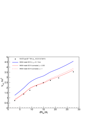
Figure 1: The pion interferometry volume dependency on the charged particles multiplicity at $p_{T}=0.2-0.3$ GeV/c. The LHC ALICE data alice_pp are compared with pure HKM results (blue solid line) and with the quantum corrected ones (red lines).

The results of Ref. SinShap are presented in the non-relativistic approximation related to the rest frame of the source moving with four-velocity $u^{\mu}$. In the hydrodynamic/hydrokinetic approach the role of such a source at a given pair’s half-momentum bin near some value $p$ is played by the fluid element or piece of the matter with the size equal to the homogeneity length $\lambda(p)$ Sin . These lengths are extracted from the HKM simulations, namely, from the interferometry radii defined by the Gaussian fits to the correlation functions obtained in HKM. All the pairs in procedure (1) are considered in the longitudinally co-moving system (LCMS) that in the boost-invariant approximation automatically selects the longitudinal rest frame of the source and longitudinal homogeneity length in this frame (it is Lorentz-dilated as compared to one in the global system Sinyuk ). The femtoscopy analysis is typically related to a fixed $p_{T}$ bin and so one needs also to determine the transverse source size in the transverse rest frame. The corresponding Lorentz transformations do not change the side-homogeneity length; as for the out-direction we proceed in the way proposed in Ref. Sinyuk .

Remaining within the Gaussian approximation, realized for expanding inhomogeneous systems in the saddle point method Sin ; AkkSin , let us fix some $\textbf{p}=(\textbf{p}_{T},0)$ in the basic LCMS reference system (basic-RS) and select the transversely moving reference systems (marked by the sign tilde) where the emission density distribution, related to the space-time center of this local source $\tilde{x}_{0i}(p)$, $\tilde{t}_{0}(p)$, can be well approximated as the following

$$\rho(x,t)\propto e^{-{\sum}_{i}\tilde{x}_{i}^{2}/2\tilde{\lambda}_{i}^{2}(p)-\tilde{t}^{2}/2\tilde{T}^{2}(p)}$$ (3)

Then in tilde-RS the correlation function has the form (2) where $R_{long}^{2}=\lambda_{long}^{2}$, $R_{side}^{2}=\lambda_{side}^{2}$, $R_{out}^{2}\rightarrow\tilde{R}_{out}^{2}=\tilde{\lambda}_{out}^{2}+\frac{\tilde{p}_{out}^{2}}{\tilde{p}_{0}^{2}}\tilde{T}^{2}$ with $\tilde{T}$ defining the duration of emission in this tilde-RS. The pair’s half-momentum $p$ corresponds to the concrete experimental bin taken in the basic-RS, the difference of the particle momenta $q$ components in selected tilde-RS are $\tilde{q}_{out}$, $\tilde{q}_{side}=q_{side}$, $\tilde{q}_{long}=q_{long}$. Therefore, only $q_{out}$ and correspondingly $R_{out}$, including $\lambda_{out}$ and $T$, are really transformed in (2) at the Lorentz boosts along the transverse momentum of the pair. The correlation function $C(p,q)$ is the Lorentz invariant, therefore $\tilde{R}_{out}^{2}(p)\tilde{q}_{out}^{2}=$ inv.

To relate the interferometry radius in the rest frame of the source (marked by the asterisk) to the one in basic-RS one should express both values through the radius in tilde-RS using the invariance property similar as it is done in Sinyuk . Then one can get

$$R^{*}_{out}(p) = R_{out}(p)\frac{\cosh y_{T}}{\cosh(y_{T}-\eta_{T})},\,R^{*}_{side}=R_{side},\,R^{*}_{long}=R_{long}$$ (4)

$$\lambda^{*}_{out} = \lambda_{out}\frac{\cosh y_{T}}{\cosh(y_{T}-\eta_{T})},\,\frac{p^{*}_{out}}{p^{*}_{0}}T^{*}=T\frac{\sinh y_{T}}{\cosh(y_{T}-\eta_{T})}$$

Here $\eta_{T}$ is a rapidity of the source in transverse direction, $y_{T}=(y_{1T}+y_{2T})/2$ is half-sum of transverse rapidities of the particles forming the pair. Then one can represent the correlation function again in the form (2) where all the variables are related already to the rest frame of the source and the HBT radii in this rest frame are expressed through the radii in basic-RS according to (4). Note that $y^{*}_{T}=y_{T}-\eta_{T}$, and if the rapidity of the pair is equal to the rapidity of the source, $y^{*}_{T}=0$, then in this particular case the radius in the rest frame is Lorentz-dilated by the factor $\gamma$. Generally, the reference system where the pair’s momentum is zero does not coincide with the rest frame of the source that emits the pair. Therefore, the direct application of these formulas is not an easy task for the rather complicated emission structure in a hypothetical hydrodynamic/hydrokinetic model of $p+p$ collisions. In Fig.2 one can see the structure of the chemical freeze-out hypersurface with the maximum value of collective velocity labeled for high multiplicity $p+p$ events in comparison with the ones for central Pb+Pb collisions at LHC. Of course, the details of the transformation will be different for a string-based event generator, therefore we present the analysis for the radii transformation just in the two limiting cases $R^{*}_{out}=R_{out}$ and $R^{*}_{out}=\gamma R_{out}$ ($\gamma=\cosh y_{T}$).

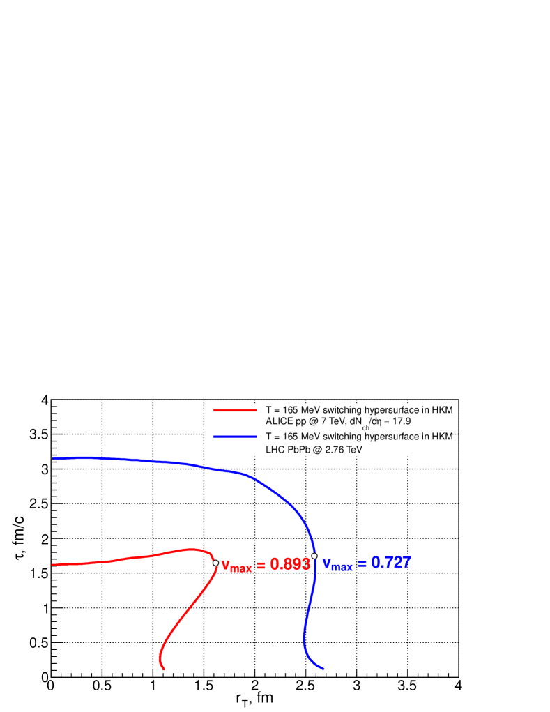
Figure 2: The chemical freeze-out hypersurface in HKM in the transverse plane for $\sqrt{s}=7$ TeV $p+p$ collisions at $\frac{dN_{ch}}{d\eta}=17.9$ (red line) in comparison with the analogous result scaled in both $\tau,r_{T}$ coordinates by the factor 1/3 for $\sqrt{s}=2.76$ TeV Pb+Pb collisions (blue line). The maximal initial energy densities are close in both cases. The maximal velocities are marked in the corresponding points on the curves.

We provide the quantum corrections at each $p_{T}$ bin in the rest frame of the corresponding source using Eq. (4) and then come back again to the basic-RS. To preserve the previous notations one can suppose that the source rest frame coincides with tilde-RS. In what follows the tilde and asterisk marks are omitted and all values are related to the source rest frame. To account that due to the uncertainty principle the emitters (strictly speaking emitted wave packets) have finite sizes $\left\langle(\Delta x)^{2}\right\rangle\sim k^{-2}$ ($k$ is the momentum variance of the particle radiation) when defining the lengths of coherence, one should at first consider the amplitude of the radiation processes and only then make statistical averaging over phases of the wave packets using the overlap integral as the coherence measure SinShap .

Following SinShap we present the quantum state $\psi_{x_{i}}(p,t)$ corresponding to a boson with mass $m$ emitted at the time $t_{i}$ from the point ${\bf x}_{i}$ as a wave packet with momentum variance $k$ which then propagates freely:

$$\psi_{x_{i}}(p,t)=e^{ipx_{i}-iEt}e^{i\varphi(x_{i})}\tilde{f}(\textbf{p})$$ (5)

where $\varphi(x_{i})$ is some phase and $\tilde{f}$ defines the primary momentum spectrum $f(\textbf{p})$ that we take in the Gaussian form,

$$f(\textbf{p})=\tilde{f}^{2}(\textbf{p})=\frac{1}{(2\pi k^{2})^{3/2}}e^{-\frac{\textbf{p}^{2}}{2k^{2}}},$$ (6)

with the variance $k^{2}=mT$. The effective temperature of particle emission in the local rest frames in HKM, $T$, is close to the chemical freeze-out temperature $T_{ch}$.

The amplitude of the single-particle radiation from some 4-volume can be written at very large times $t_{\infty}$ as a superposition of the wave functions $\psi_{x_{i}}(p)$ with coefficients $\widehat{\rho}(x_{i})=\sqrt{\rho(x_{i})}$ that leads in the case of completely random phases to the emitter distribution (3) in the local rest frames of the sources:

$$A(p,t)=c\int d^{4}x_{i}\psi_{x_{i}}(p,t)\widehat{\rho}(x_{i}),$$ (7)

where $c$ is the normalization constant.

In the paper SinShap the two-particle state is considered as a product of the single-particle amplitudes, thus suggesting the maximal possible distinguishability and independence of different emitters compatible with the uncertainty principle for momentum & position and energy-momentum & time measurements. The latter is accounted for by the averaging of such a two-particle amplitude over partially coherent phases between different emitters with overlap integral measure Tolst ; SinShap .

With that said the single- and two-particle spectra, averaged over the ensemble of emission events with partially correlated phases $\varphi(x)$ are

$$\overline{W(p)} = c^{2}\int d^{4}xd^{4}x^{\prime}e^{ip(x-x^{\prime})}\widehat{\rho}(x)\widehat{\rho}(x^{\prime})f(\textbf{p})\langle e^{i(\varphi(x)-\varphi(x^{\prime}))}\rangle$$

$$\overline{W(p_{1},p_{2})} = c^{4}\int d^{4}x_{1}d^{4}x_{2}d^{4}x_{1}^{\prime}d^{4}x_{2}^{\prime}e^{i(p_{1}x_{1}+p_{2}x_{2}-p_{1}x_{1}^{\prime}-p_{2}x_{2}^{\prime})}\cdot$$ (8)

$$\cdot f(\textbf{p}_{1})f(\textbf{p}_{2})\widehat{\rho}(x_{1})\widehat{\rho}(x_{2})\widehat{\rho}(x_{1}^{\prime})\widehat{\rho}(x_{2}^{\prime})\langle e^{i(\varphi(x_{1})+\varphi(x_{2})-\varphi(x_{1}^{\prime})-\varphi(x_{2}^{\prime}))}\rangle.$$

The phase averages are associated with corresponding overlap integrals SinShap

$$\langle e^{i(\varphi(x)-\varphi(x^{\prime}))}\rangle = G_{xx^{\prime}}=I_{xx^{\prime}}=\left|\int d^{3}{\bf r}\psi_{x}(t,{\bf r})\psi_{x^{\prime}}^{*}(t,{\bf r})\right|,$$ (9)

$$\langle e^{i(\varphi(x_{1})+\varphi(x_{2})-\varphi(x_{1}^{\prime})-\varphi(x_{2}^{\prime}))}\rangle = G_{x_{1}x_{1}^{\prime}}G_{x_{2}x_{2}^{\prime}}+G_{x_{1}x_{2}^{\prime}}G_{x_{2}x_{1}^{\prime}}-G_{x_{1}x_{2}^{\prime}}G_{x_{2}x_{1}^{\prime}}G_{x_{1}x_{2}}$$ (10)

where $\psi_{x_{i}}(t,{\bf r})=\frac{1}{(2\pi)^{3/2}}\int f(\textbf{p})e^{-i{\bf p(r-x}_{i})}e^{-i\frac{{\bf p}^{2}}{2m}(t_{i}-t)}d^{3}p$   are the wave functions of single bosonic states in coordinate representation.

Then the correlation function $C({\bf p},{\bf q})$ can be expressed through the homogeneity lengths in the local rest frame $R_{L}\equiv\lambda_{long}^{*}(p)$, $R_{S}\equiv\lambda_{side}^{*}(p)$, $R_{O}\equiv\lambda_{out}^{*}(p)$ that are expressed through the HBT radii obtained from the Gaussian fit (2) of the HKM correlation functions and transformation law (4) as described above.

$$C({\bf p},{\bf q})=\frac{\overline{W(p_{1},p_{2})}}{\overline{W(p_{1})}\overline{W(p_{2})}}=$$ (11)

$$= 1+e^{-q_{O}^{2}R_{O}^{2}\frac{4k_{0}^{2}R_{O}^{2}}{1+4k_{0}^{2}R_{O}^{2}}-q_{S}^{2}R_{S}^{2}\frac{4k_{0}^{2}R_{S}^{2}}{1+4k_{0}^{2}R_{S}^{2}}-q_{L}^{2}R_{L}^{2}\frac{4k_{0}^{2}R_{L}^{2}}{1+4k_{0}^{2}R_{L}^{2}}-\frac{({\bf q}\cdot{\bf p})^{2}T^{2}}{m^{2}}\frac{4k^{2}T^{2}}{1+4k^{2}T^{2}}}-C_{d}({\bf p},{\bf q}),$$

where $k_{0}^{2}=k^{2}/(1+\alpha k^{4}T^{2}/m^{2})$, parameter $\alpha(k^{2}R^{2})$ is defined from the model numerically (it is the order of unity for $R\sim 1$ fm and tends to zero for the large sources – see SinShap for details), and the subtracted term

$$C_{d}({\bf p},{\bf q})=e^{-\frac{2q_{O}^{2}k_{0}^{2}R_{O}^{4}\left(1+8k_{0}^{2}R_{O}^{2}\right)}{\left(1+4k_{0}^{2}R_{O}^{2}\right)\left(1+8k_{0}^{2}R_{O}^{2}+8k_{0}^{4}R_{O}^{4}\right)}-\frac{2q_{S}^{2}k_{0}^{2}R_{S}^{4}\left(1+8k_{0}^{2}R_{S}^{2}\right)}{\left(1+4k_{0}^{2}R_{S}^{2}\right)\left(1+8k_{0}^{2}R_{S}^{2}+8k_{0}^{4}R_{S}^{4}\right)}-\frac{2q_{L}^{2}k_{0}^{2}R_{L}^{4}\left(1+8k_{0}^{2}R_{L}^{2}\right)}{\left(1+4k_{0}^{2}R_{L}^{2}\right)\left(1+8k_{0}^{2}R_{L}^{2}+8k_{0}^{4}R_{L}^{4}\right)}}\cdot$$

$$\cdot e^{-\frac{2k^{2}T^{4}({\bf p}\cdot{\bf q})^{2}\left(1+8k^{2}T^{2}\right)}{m^{2}\left(1+4p^{2}T^{2}\right)\left(1+8k^{2}T^{2}+8k^{4}T^{4}\right)}}F(k_{0}^{2}R_{i}^{2},k^{2}T^{2}),$$

$$F(k_{0}^{2}R_{i}^{2},k^{2}T^{2})=\left(\frac{k_{0}}{k}\right)^{3/2}\left(\frac{1+4k^{2}T^{2}}{1+8k^{2}T^{2}+8k^{4}T^{4}}\frac{1+4k_{0}^{2}R_{O}^{2}}{1+8k_{0}^{2}R_{O}^{2}+8k_{0}^{4}R_{O}^{4}}\cdot\right.$$

$$\left.\cdot\frac{1+4k_{0}^{2}R_{S}^{2}}{1+8k_{0}^{2}R_{S}^{2}+8k_{0}^{4}R_{S}^{4}}\frac{1+4k_{0}^{2}R_{L}^{2}}{1+8k_{0}^{2}R_{L}^{2}+8k_{0}^{4}R_{L}^{4}}\right)^{1/2}$$ (12)

corresponds to the elimination of the double counting.

Now we can see that the apparent interferometry radii extracted from the Gaussian fits to the correlation function (11) are reduced as compared to those obtained in the standard approach.

Particularly, if we neglect the double counting effects, truncate the subtracted term $C_{d}({\bf p},{\bf q})$ in (11), and fit the correlation function with the Gaussian (2), we obtain the femtoscopic radii $R_{out}$, $R_{side}$, $R_{long}$ related to the standard ones $R_{out,st}$, $R_{side,st}$, $R_{long,st}$ as follows

$$\frac{R^{2}_{out}}{R_{out,st}^{2}} = \left(R_{O}^{2}\frac{4k_{0}^{2}R_{O}^{2}}{1+4k_{0}^{2}R_{O}^{2}}+T^{2}v^{2}_{out}\frac{4k^{2}T^{2}}{1+4k^{2}T^{2}}\right)/\left(R_{O}^{2}+T^{2}v^{2}_{out}\right)$$

$$\frac{R^{2}_{side}}{R_{side,st}^{2}} = \frac{4k_{0}^{2}R_{S}^{2}}{1+4k_{0}^{2}R_{S}^{2}}$$ (13)

$$\frac{R^{2}_{long}}{R_{long,st}^{2}} = \frac{4k_{0}^{2}R_{L}^{2}}{1+4k_{0}^{2}R_{L}^{2}}$$

where $v_{out}=p^{*}_{out}/p_{0}^{*}\ll 1$ according to the non-relativistic approximation. For large source sizes, e.g. when the homogeneity lengths correspond to $A+A$ collisions, $k_{0}^{2}R^{2}\gg 1$, $k^{2}T^{2}\gg 1$, all these ratios tend to unity.

The mean emission duration is supposed to be proportional to the average system size, $T=a(R_{O}+R_{S}+R_{L})/3$ that leads to a quadratic equation expressing $R_{O}$ (and $T$) through $R_{i,st}$. The latter are connected with ones taken in the basic-RS according to transformation laws (4). The value $a$ is a free model parameter. Then we put these extracted values into the expression (11) for the correlation function and perform its fitting with the Gaussian (2). This gives us finally the interferometry radii $R_{out}$, $R_{side}$ and $R_{long}$ in view of the uncertainty principle. The radii are presented then in the basic-RS using the transformations inverse to (4).

The correlation function is the ratio of the two- and one-particle spectra. It is found SinShap that quantum corrections to this ratio are not so sensitive to different forms of the wave packets as the spectra itself. In particular, the effective temperature of the corrected transverse spectra depends on whether the parameter of mean particle momentum is included or not into the wave packet formalism. If yes, the corrected effective temperature for small sources $R\sim 1$ fm is equal or even higher than that of individual emitters, $T=k^{2}/m$, while for the wave packets in the form (5) it is lower SinShap . Besides of this, in the non-relativistic approximation one can describe only very soft part of the spectra. That is why we focus in the Letter on the corrections to the Bose-Einstein correlation functions where in the rest frame of the source the total and relative momenta of the boson pairs are fairly small.

IV The results for $p+p$ and $p+\textrm{Pb}$ collisions, and discussion

The initial conditions for HKM are described in Section 2. The HKM event generator provides us with the interferometry radii in basic-RS. To find the corresponding homogeneity lengths in the rest frame of the source according to (4) we use, as discussed in Section 3, the two limiting cases: the transverse boost to the rest frame of the pair from the basic LCMS system, or no transformation at all. For the former case it is defined by the $p_{T}$ bin and for $p_{T}=0.2-0.3$ GeV $\cosh y_{T}=\gamma=2.05$. The parameter $a$ connecting $T$ with $R_{i}$ increases linearly with multiplicity from 0.8 to 1.0, primary momentum spectrum dispersion $k=0.16$ GeV/c (T=0.18 GeV), pair mean transverse momentum in the source rest frame $p^{*}_{T}=0.15$ GeV/c. The $\alpha$ parameter is set to linearly decrease with multiplicity from 0.8 to 0.6. As for the $\gamma=1$ case, the parameter $a$ decreases linearly with multiplicity from 1.1 to 0.9, $k=0.18$ GeV/c and $p^{*}_{T}=0.13$ GeV/c. The $\alpha$ parameter decreases linearly with multiplicity from 1.35 to 0.9 which is close to the theoretical results SinShap .

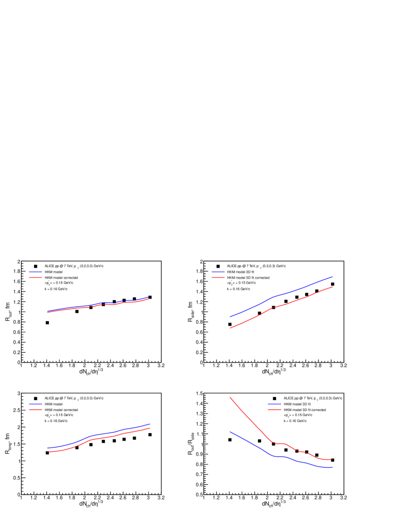
Figure 3: The pion interferometry radii dependency on charged particles multiplicity

at $p_{T}=0.2-0.3$ GeV/c. The designations are the same as in Fig. 1.

In Fig. 1 along with the experimental and pure HKM results we present the multiplicity dependence of the quantum corrected interferometry volume at $p_{T}=0.25$ GeV/c. The solid line represents the corrected values calculated under the assumption that the $R_{out}$ interferometry radii, observed in basic-RS, are Lorentz-contracted by a factor $\gamma=2.05$ for the chosen $p_{T}=0.25$ GeV/c value as compared to ones in the source rest system. The dashed line demonstrates the no-contraction case when $\gamma=1$. As one can see the accounting for the uncertainty principle allows one to describe the overall multiplicity dependence of the interferometric radii. Figure 3 represents the dependence on multiplicity of individual radius parameters.

The suppression of the Bose-Einstein correlations for small sources with closely located emitters takes place even without specific coherence mechanism and resonance contributions. To see this effect the double counting in the correlation function should be eliminated as Eq. (11) demonstrates. Then the additional suppression parameter $\lambda_{\text{c}oh}<1$ in the Gaussian fit appears and the relevant parameter in (2) becomes $\lambda=\lambda_{\text{c}oh}\lambda_{\text{HKM}}$. The result of our calculations gives $\lambda_{coh}=$ 0.9 – 0.95 for not very small multiplicities.

In addition to the correlation analysis of $p+p$ collisions, let us make the simplest estimates and try to predict the HBT radii for $p+$Pb collisions at the LHC energy $\sqrt{s}=5.02$ GeV. We ignore the possible asymmetry of the hydrodynamic tube in the longitudinal direction and present our prediction within hHKM for centrality $c=0-20$ % with $dN_{ch}/d\eta$ = 35. The results are calculated for the two initial radii with rms equal to 0.9 fm and 1.5 fm and also for the two initial times: $\tau=$ 0.1 fm/c and 0.25 fm/c. It turns out that the latter factor is not essential if we keep fixed final multiplicity: only the longitudinal radii are 3–4% higher at $\tau=$ 0.25 fm/c than at 0.1 fm/c. The transverse radii practically coincide. Therefore, we finally demonstrate only the case $\tau=$ 0.1 fm/c. The initial transverse sizes of the system, created in the $p+$Pb collision, are taken from Ref. Boz : “In the conventional wounded nucleon model it is assumed that the sources are located in the transverse plane in the centers of the participating nucleons. This amounts to rather large initial transverse sizes in the $p-$Pb system, $R=1.5$ fm. Locating the source in the center-of-mass of the $NN$ system is also admissible, which leads to a more compact initial distribution, $R=0.9$ fm”. The results for the interferometry volume are presented in Fig. 4. The model parameter set is extrapolated from the described above and consistent with that for the $p+p$ system, with $\gamma=1$ to the case of larger sizes typical for the $p+$Pb collisions. At that the $k$ and $p^{*}_{T}$ values are left the same as for the $p+p$ case, whereas $\alpha$ and $a$ are chosen to be smaller. For the $R=0.9$ fm initial transverse size $\alpha=0.5$, $a=0.7$ and for $R=1.5$ fm we put $\alpha=0.45$, $a=0.6$.

Considering the multiplicity dependence of femtoscopy scales in $p+p$ and $p+$Pb collisions we cannot bypass the scaling hypothesis issue Lisa , that suggests a universal linear dependence of the HBT volume on the particle multiplicity. It means that the observed interferometry volume depends roughly only on the multiplicity of particles produced in collision, but not on the geometrical characteristics of the collision process. At the same time, as it was found in the theoretical analysis in Ref. scaling , the interferometry volume should depend not only on the multiplicity, but also on the initial size of colliding systems. In more detail, the intensity of the transverse flow depends on the initial geometrical size $R^{g}_{0}$ of the system: roughly, if the pressure is $p=c_{0}^{2}\epsilon$, then the transverse acceleration $a=\nabla_{x_{T}}p/\epsilon\propto p({\bf x}_{T}=0)/(R_{0}^{g}\epsilon)=c_{0}^{2}/R^{g}_{0}$. The interferometry radii $R_{T}$, that are associated with the homogeneity lengths, depend on the velocity gradient and geometrical size, and for non-relativistic transverse expansion can be approximately expressed through $R^{g}_{0}$, the averaged transverse velocity $\left\langle|v_{T}|\right\rangle$ and inverse of the temperature $\beta$ at some final moment $\tau$ AkkSin ; Csorgo ; PBM :

$$R_{T}=\frac{R^{g}(\tau)}{\sqrt{1+\frac{2}{\pi}\langle|v_{T}|\rangle^{2}\beta m_{T}}}\approx R_{0}^{g}\left(1+\frac{\tau^{2}c_{0}^{2}}{2\left(R^{g}_{0}\right)^{2}}-\beta m_{T}\frac{\tau^{2}c^{2}_{0}}{\pi^{2}\left(R^{g}_{0}\right)^{2}}\right)$$ (14)

The result (14) for the HBT radii depends obviously on $R_{0}^{g}$ and, despite its roughness, demonstrates the possible mechanism of compensation of the growing (in time) geometrical radii of an expanding fireball in the femtoscopy measurements. For some dynamical models of expanding fireballs Csorgo2 the interferometry radii, measured at the final time of system’s decoupling, are fully coincided with the initial geometrical ones, no matter how large the multiplicity is. The reason for such a behavior is explained in Ref. HKM : if there is no dissipation in the expanding system, namely, the evolution corresponds to a solution of the Boltzmann equation with $F^{gain}(t,{\bf x})=F^{loss}(t,{\bf x})$, then the spectra and correlation functions are coincided with the initial ones. The detail study of hydrodynamically expanding systems is provided in Ref. scaling . It is found that at the boost-invariant isentropic and chemically frozen evolution the interferometry volume, if it were possible to measure the interferometry radii at some evolution time $\tau$, is approximately constant:

$$V_{int}(\tau)\simeq C(\sqrt{s})\frac{dN/dy(\tau)}{\langle f\rangle_{\tau}T_{eff}^{3}(\tau)}$$ (15)

where $\left\langle f\right\rangle$ is the averaged phase-space density Bertsch which is found to be approximately conserved during the hydrodynamic evolution under above conditions as well as $\frac{dN}{dy}$ scaling . As for the effective temperature of the hadron spectra, $T_{eff}(\tau)=T(\tau)+m\frac{\left\langle v_{T}(\tau)\right\rangle^{2}}{2}$, one can see that when the system’s temperature $T$ drops, the mean $v_{T}^{2}$ increases, therefore $T_{eff}$ does not change much during the evolution (it slightly decreases with time for pions and increases for protons). Hence $V_{int}$, if it has been measured at some evolution time $\tau$, will also approximately conserve. Of course, the real evolution is neither isentropic, nor chemically frozen, includes also QGP stage, but significant dependence of the femtoscopy scales on the initial system size is preserved anyway.

Fig. 4 shows the dependency $V_{int}(\langle dN_{ch}/d\eta\rangle)$ for the case of $p+p$ collisions at the LHC, $\sqrt{s}=7$ TeV, and for the most central (only!) collisions of nuclei having similar sizes, Pb+Pb and Au+Au, at the SPS, RHIC and LHC. We have also added on the plot our prediction for the interferometry volume of $p$Pb system, that has an initial size larger than that for the $pp$ system. As one can see, the different groups of points corresponding to $p+p$, $p+$Pb and $A+A$ events cannot be fitted by the same straight line. This apparently confirms the result obtained in scaling that the interferometry volume is a function of both variables: the multiplicity and the initial size of colliding system. The latter depends on the atomic number $A$ of colliding objects and the collision centrality $c$.

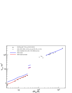
Figure 4: The interferometry volume dependency on charged particles multiplicity. The curve fragments in the middle correspond to the HKM prediction for $p+$Pb collision at the LHC energy $\sqrt{s}=5.02$ GeV. The upper one is related to the initial transverse system size $R=1.5$ fm and for the two lower ones $R=0.9$ fm. The curves at the left and at the right represent the HKM results for $p+p$ and $A+A$ central collisions respectively, compared to the experimental data at AGS, SPS, RHIC and LHC, taken from papers alice_pp , AaExp1 – AaExp8 . The $pp$ volumes are calculated as a product $R_{out}R_{side}R_{long}$ of respective experimental radii. The blue lines correspond to pure HKM results, whereas the quantum corrections to them are presented by the red lines.

In Figs. 5 and 6 for the two multiplicity classes $\langle dN_{ch}/d\eta\rangle=9.2$ and $\langle dN_{ch}/d\eta\rangle=17.9$ we present the three curves for interferometry radii as a function of $p_{T}$: the experimental one, the one taken just from the HKM simulations and the other one obtained after application of the quantum corrections. The basic parameters used correspond to the case $\gamma=1$ (see above). The $\alpha$ parameter values linearly increase with $p_{T}$ from 1.15 to 1.35 for the $\langle dN_{ch}/d\eta\rangle=9.2$ case and from 1.02 to 1.10 for $\langle dN_{ch}/d\eta\rangle=17.9$ in such a way that for $p_{T}$ bin (0.2,0.3) it has the same values as in previous $R_{i}(\langle dN_{ch}/d\eta\rangle)$ calculations. As one can see, similarly to the multiplicity behavior, the quantum corrected $p_{T}$-dependency of the radii also gets closer to the experimental values, but for large $p_{T}$ the corrections are insufficient to fully describe the observable femtoscopy scales behavior. This fact may indicate that sources of particles with large $p_{T}$ cannot be described in hydrodynamical approximation. Note that just for such large $p_{T}$ the non-trivial base-line corrections, already provided in presented experimental data, are very essential.

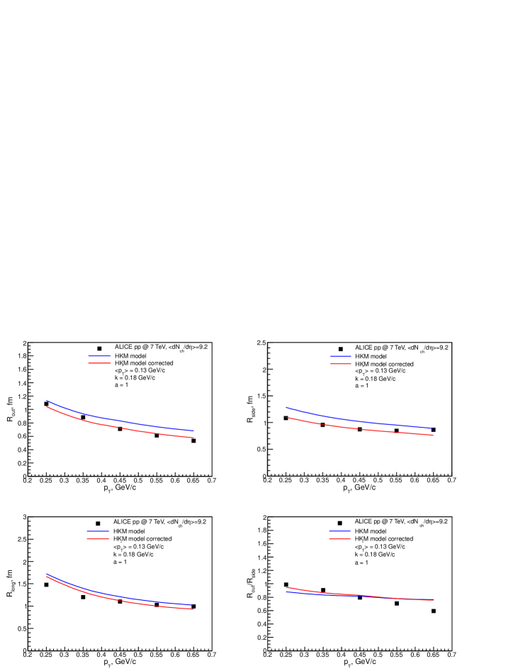
Figure 5: Dependence of interferometry radii on $p_{T}$, $\langle dN_{ch}/d\eta\rangle=9.2$

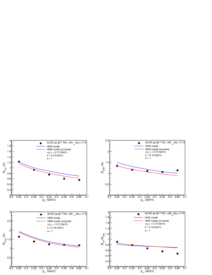
Figure 6: Dependence of interferometry radii on $p_{T}$, $\langle dN_{ch}/d\eta\rangle=17.9$

Finally we demonstrate the prediction of the $p_{T}$-dependence of the radii for $p+$Pb collisions. It is presented in Fig.7 together with the corrections due to the uncertainty principle. One can see that corrections are smaller for the systems with larger homogeneity lengths and not very essential for $p+$Pb and probably for $A+A$ peripheral collisions. As for the homogeneity lengths formation, in a very recent paper Bzdak it is found that, in the absence of hydrodynamic flow, the HBT radii should be similar in $pp$ and $p$Pb collisions.

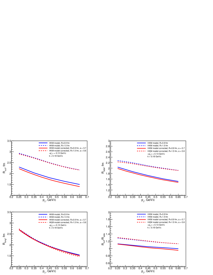
Figure 7: The HKM prediction for the dependence of $p+$Pb interferometry radii on $p_{T}$ at the LHC energy $\sqrt{s}=5.02$ GeV, $\langle dN_{ch}/d\eta\rangle=35$.

V Conclusions

One can conclude that quantum corrections to pion interferometry radii in $p+p$ collisions at the LHC can significantly improve the (semi-classical) event generator results that typically give an overestimate of the experimental interferometry radii and volumes. The corrections account for the basic (partial) indistinguishability and mutual coherence of closely located emitters because of the uncertainty principle SinShap . The additional suppression of the Bose-Einstein correlation function also appears. The effects become important for small sources, 1–2 fm or smaller. Such systems cannot be completely random and so require a modification of the standard theoretical approach for correlation analysis. The predicted interferometric radii for $p+$Pb collisions need some small corrections only for its minimal values corresponding to the initial transverse size of $p$Pb system 0.9 fm.

More sophisticated result of this study is a good applicability of the hydrodynamics/hydrokinetics with the quantum corrections for description of HBT radii not only in $A+A$ collisions but also, at least for large multiplicities, in $p+p$ events. These radii are well reproduced for not too large $p_{T}$. Whether it means the validity of the hydrodynamic mechanism for the bulk matter production in the LHC $p+p$ collisions is still an open question. It is also related to the problem of early thermalization in the processes of heavy ion collisions; the nature of this phenomenon is still a fundamental theoretical issue.

VI Acknowledgment

Yu.M.S. is grateful to B. Kopeliovich, R. Lednický, L.V. Malinina, E.E. Zabrodin for fruitful discussions and to the ExtreMe Matter Institute EMMI for visiting professor position. Iu.A.K. acknowledges the financial support by the ExtreMe Matter Institute EMMI and Hessian LOEWE initiative. The research was carried out within the scope of the EUREA: European Ultra Relativistic Energies Agreement (European Research Group: “Heavy ions at ultrarelativistic energies”), and is supported by the State Fund for Fundamental Researches of Ukraine (Agreement F33/24-2013).

References

- (1) G.Goldhaber, S.Goldhaber, W. Lee, A. Pais, Phys. Rev. 120 (1960) 325.
- (2) G.I. Kopylov, M.I. Podgoretsky, Sov. J. Nucl. Phys.: 15 (1972) 219; 15 (1972) 219 18 (1973) 336; 19 (1974) 215.
- (3) S. Pratt, Phys. Rev. D 33 (1986)1314.
-
(4)
A.N. Makhlin, Yu.M. Sinyukov, Sov. J. Nucl. Phys. 46 (1987) 345;
A. N. Makhlin, Yu. M. Sinyukov, Z. Phys. C 39 (1988) 69. - (5) Yu. M. Sinyukov, Nucl. Phys. A 498 (1989) 151.
- (6) Y. Hama, S.S. Padula, Phys. Rev. D 37 (1988) 3237.
-
(7)
Yu.M. Sinyukov, Nucl.Phys. A 566 (1994) 589c;
Yu.M. Sinyukov, in: Hot Hadronic Matter: Theory and Experiment, eds. J. Letessier, H.H. Gutbrod and J. Rafelski (Plenum, New York) 1995, 309. - (8) S.V. Akkelin, Yu.M. Sinyukov, Phys. Lett. B 356 (1995) 525; S.V. Akkelin, Yu.M. Sinyukov, Z. Phys. C 72 (1996) 501.
- (9) Yu.M. Sinyukov, S.V. Akkelin, Iu.A. Karpenko. Act. Phys. Pol. 40 (2009) 1025.
- (10) Yu.M.Sinyukov, R.Lednický, J.Pluta, B.Erazmus, S.V.Akkelin. Phys. Lett. B 432 (1998) 248.
- (11) Gordon Baym, Peter Braun-Munzinger, Nucl, Phys. A 610 (1996) 286c.
- (12) Yu. M. Sinyukov, V. M. Shapoval, Phys.Rev. D 87 (2013) 094024, arXiv:1209.1747.
- (13) M.S. Nilsson, L.V. Bravina, E.E. Zabrodin, L.V. Malinina,J. Bleibel, U. Mainz. Phys.Rev. D 84 (2011) 054006.
- (14) Q. Li, G. Graef, M. Bleicher, arXiv: 1209.0042 [hep-ph], 2012.
- (15) P. Bozek, Acta Phys. Pol. B41 (2010) 837.
- (16) K. Werner et al, Phys.Rev. C 83 (2011) 044915.
- (17) Yu.M. Sinyukov, S.V. Akkelin, and Y. Hama, Phys. Rev. Lett. 89 (2002) 052301.
- (18) S.V. Akkelin, Y. Hama, Iu.A. Karpenko, Yu.M. Sinyukov. Phys. Rev. C 78 (2008) 034906. Iu.A. Karpenko, Yu.M. Sinyukov. Phys. Rev. C 81 (2010) 054903.
- (19) Iu.A. Karpenko, Yu.M. Sinyukov, K. Werner. Phys.Rev. C 87 (2013) 024914.
- (20) L.D. Landau, Izv. Akad. Nauk SSSR, Ser. Fiz. 17 (1953) 51.
- (21) Edward K.G. Sarkisyan, Alexander S. Sakharov, Eur. Phys. J. C 70 (2010) 533-541.
- (22) Edward K.G. Sarkisyan, Alexander S. Sakharov, AIP Conf. Proc. 828 (2006) 35-41, arXiv:hep-ph/0510191.
- (23) M. Laine, Y. Schroder, Phys. Rev. D 73 (2006) 085009.
- (24) K. Nakamura et al. (Particle Data Group), J. Phys. G 37, 075021 (2010) and 2011 partial update for the 2012 edition.
- (25) S.A. Bass et al., Prog. Part. Nucl. Phys. 41 (1998) 255; Prog. Part. Nucl. Phys. 41 (1998) 225; M. Bleicher et al., J. Phys. G 25 (1999) 1859.
-
(26)
B.Z. Kopeliovich , A. Sch¨afer, and A. V. Tarasov, Phys. Rev. D 62 (2000) 054022;
E. Shuryak and I. Zahed, Phys. Rev. D 69 (2004) 014011. - (27) S. Pratt, Phys. Rev. C 56 (1997) 1095.
- (28) K. Aamodt, et al. (ALICE Collaboration), Phys. Rev. D 84 (2011) 112004.
- (29) B. Lorstad, Yu.M. Sinyukov, Phys. Lett. B 256 ( 1991 ) 159.
- (30) R. Lednický, V.L. Lyuboshits, M.I. Podgoretsky. J.Nucl Phys. 38 (1983) 251.
- (31) Yu.M.Sinyukov, A.Yu.Tolstykh. Z.Phys.C – Particles and Fields 61 (1994) 593.
- (32) P. Bozek and P. Broniowski arXiv:1301.3314 (2013).
-
(33)
M. Lisa, S. Pratt, R. Soltz, U. Wiedemann. Ann.Rev.Nucl.Part.Sci. 55 (2005) 357;
M. Lisa Braz.J.Phys. 37 2007 963. -
(34)
S.V. Akkelin, Yu.M. Sinyukov, Phys. Rev. C 70 (2004) 064901;
S.V. Akkelin, Yu.M. Sinyukov, Phys. Rev. C 73 (2006) 034908. - (35) T. Csorgo and B. Lorstad, Lund Preprint LUNFD6 (NFPL-7082), 1994.
- (36) S.V. Akkelin, P. Braun-Munzinger, Yu.M. Sinyukov, Nucl. Phys. A 710 (2002) 439.
- (37) P. Csizmadia, T. Csorgo, and B. Lukacs, Phys. Lett. B 443 (1998) 21.
- (38) G.F. Bertsch, Phys. Rev. Lett. 72 (1994) 2349; 77 (1996) 789.
- (39) A. Bzdak, B. Schenke, P. Tribedy, R. Venugopalan, arXiv:1304.3403 (2013).
- (40) K. Aamodt, et al (ALICE Collaboration). Phys.Lett. B 696 (2011) 328.
- (41) Dariusz Antonczyk. Acta Phys. Polon. B 40 (2009) 1137.
- (42) S.V. Afanasiev et al, NA49 Collaboration. Phys. Rev. C 66 (2002) 054902.
- (43) C. Alt et al, NA49 Collaboration. Phys.Rev. C 77 (2008) 064908.
- (44) J. Adams et al. (STAR Collaboration). Phys.Rev.Lett. 92 (2004) 112301.
- (45) J. Adams et al. (STAR Collaboration). Phys.Rev. C 71 (2004), 044906.
- (46) S.S. Adler et al. (PHENIX Collaboration). Phys.Rev. C 69 (2004) 034909.
- (47) S.S. Adler et al. (PHENIX Collaboration). Phys.Rev.Lett. 93 (2004) 152302.