The Persistent Activity of Jupiter-Family Comets at 3 to 7 AU

Abstract

We present an analysis of comet activity based on the Spitzer Space Telescope component of the Survey of the Ensemble Physical Properties of Cometary Nuclei. We show that the survey is well suited to measuring the activity of Jupiter-family comets at 3–7 AU from the Sun. Dust was detected in 33 of 89 targets ($37\pm 6$%), and we conclude that 21 comets ($24\pm 5$%) have morphologies that suggest ongoing or recent cometary activity. Our dust detections are sensitivity limited, therefore our measured activity rate is necessarily a lower limit. All comets with small perihelion distances ($q<1.8$ AU) are inactive in our survey, and the active comets in our sample are strongly biased to post-perihelion epochs. We introduce the quantity $\epsilon f\rho$, intended to be a thermal emission counterpart to the often reported $Af\rho$, and find that the comets with large perihelion distances likely have greater dust production rates than other comets in our survey at 3–7 AU from the Sun, indicating a bias in the discovered Jupiter-family comet population. By examining the orbital history of our survey sample, we suggest that comets perturbed to smaller perihelion distances in the past 150 yr are more likely to be active, but more study on this effect is needed.

1 Introduction

The Survey of the Ensemble Physical Properties of Cometary Nuclei (SEPPCoN) provides a data set with which we may examine comet activity at intermediate heliocentric distances, $r_{h}$ (here, 3–7 AU). The primary goal of SEPPCoN is to measure, in a consistent manner, the sizes and surface properties of a statistically significant number ($\approx 100$) of Jupiter-family comet nuclei. SEPPCoN is comprised of two observational campaigns: a mid-infrared (mid-IR) component utilizing the imaging capabilities of the Spitzer Space Telescope (Werner et al. 2004), and a visible light component using ground-based instrumentation. Early results from the Spitzer survey on Comets 22P/Kopff and 107P/Wilson-Harrington were presented by Groussin et al. (2009) and Licandro et al. (2009), respectively. Fernández et al. (2011), hereafter Paper I, presented the first survey results from SEPPCoN. In Paper I, we measured and analyzed the thermal emission from 89 comet nuclei, and presented results on the cumulative size distribution and spectral properties of the Spitzer survey targets. The goal of the present paper is to examine the dust and activity of those same targets.

Active comets produce a coma. A coma is a gravitationally unbound atmosphere, driven by the outflow of volatiles from the nucleus surface or sub-surface. As comets approach the Sun, their surfaces warm, eventually causing gases to be released from the nucleus due to sublimation of volatile ices. The heliocentric distance at which this occurs depends on the physical properties of the nucleus in question: shape, composition, and internal structure. Volatile driven mass loss due to insolation is typical of comet activity, i.e., we may not even consider an object to have cometary activity unless we observe a coma and/or tail generated by solar heating of volatiles (as opposed to impact driven mass loss). In addition to the gases, the coma typically includes escaping dust and/or icy grains lifted off the nucleus by the gas outflow. As a comet recedes from the Sun, the nucleus cools and activity may be quenched.

Water ice is typically the primary driver of comet atmospheres inside of 3 AU (Meech and Svoren̆ 2004). Water is by far the most abundant ice near the nucleus surface, as inferred from remote spectrophotometric compositional studies of comae. The next most abundant gases are CO₂ and CO with relative fractions $\lessapprox 20$% (Bockelée-Morvan et al. 2004, Ootsubo et al. 2012). However, CO₂ can also drive activity, even though it is generally less abundant than water, as shown by the Deep Impact flybys of Comets 103P/Hartley 2 (A’Hearn et al. 2011) and 9P/Tempel 1 (Feaga et al. 2007). Outside of 3 AU, the relative contributions of water ice and more volatile ices to activity is less well understood. Activity has been observed in more than 80 comets with large perihelion distances ($q>5$ AU), despite the inferred low surface temperatures at such great distances. Ices more volatile than water must play larger roles in driving activity for these distant comets than for comets closer to the Sun. Water sublimates at $T\approx 170$ K (which occurs in the solar system near $r_{h}\approx 3$ AU), whereas CO₂ ice sublimates at $T\approx 80$ K ($r_{h}\approx 12$ AU) and CO at $T\approx 20$ K ($r_{h}\approx 50$ AU). Recent results from the Akari satellite show that the coma mixing ratio of CO₂ to H₂O is systematically larger for comets outside of 2.5 AU, indicating the diminishing role of water sublimation as heliocentric distance increases (Ootsubo et al. 2012). In addition to sublimation of ices, the crystallization of amorphous water ice could release trapped gases and drive activity at 120–160 K (Schmitt et al. 1989, Meech and Svoren̆ 2004), and has been proposed as the dominant driver of activity in Centaurs (Jewitt 2009). Whatever the mechanism that drives activity in comets with $q>5$ AU, not all comets are active at such large heliocentric distances. By studying the activity of comets at intermediate heliocentric distances we may learn which properties of comet nuclei initiate activity as they approach the Sun, and quench or sustain activity as they recede from the Sun.

Mid-IR broadband images of comets, such as those taken as part of our survey, are dominated by thermal emission from the nuclei and surrounding dust. With few exceptions, the gas is undetected or only forms a minor component of the emission. Because gas expansion is a critical component to comet activity, but remains undetected in most mid-IR images, in this work we infer activity from the presence and morphology of dust structures larger than the point source nucleus, rather than from the direct detection of gases.

With SEPPCoN Spitzer images, we measure the dust activity of comet nuclei at 3–7 AU, distances where water ice sublimation is typically low. First, we review the Spitzer observations which were presented in detail in Paper I (§2). Next, we present the morphology and the photometric properties of the dust detected in the survey, and assess the nature of the dust (§3). Then, we discuss the frequency of cometary activity versus heliocentric distance and other parameters, their implications on the structure and heating of comet nuclei, and analyze the color temperature of comet dust at 3–7 AU (§4). Finally, we summarize our findings (§5).

2 Observations and Reduction

The purpose of the Spitzer component of the survey is to obtain a robust estimate of the size distribution of known Jupiter-family comet nuclei. To this end, 100 JFCs were selected that met the following criteria: 1) the ephemeris was constrained well enough such that the comet could be expected to lie within a $5\mbox{${}^{\prime}$}\times 5\mbox{${}^{\prime}$}$ field of view (the footprint of Spitzer’s largest arrays); 2) the comet must have been observable by Spitzer and beyond $\approx 4$ AU from the Sun during Spitzer Cycle 3 (July 2006 to July 2007); and, 3) the nucleus must have been brighter than $V=24.0$ mag to make ground-based optical observations feasible. Criterion 3 requires an estimate of the nucleus radius ($R$), which we obtained from the compilation of Lamy et al. (2004). If no estimate existed, we used the following assumption: $R=1.0$ km for comets with perihelion distances $q<2.0$ AU, $R=1.5$ km for $2.0<q<2.5$ AU, and $R=2.0$ km for $q>2.5$ AU. The assumption attempts to account for the fact that it is increasingly difficult to discover smaller comets at larger perihelion distances.

Two Spitzer instruments were well suited for the survey: the 24-µm ($\lambda_{eff}=23.7$ µm, 2.55 arcsec pixel^-1, $5.4\mbox{${}^{\prime}$}\times 5.4\mbox{${}^{\prime}$}$ field of view) camera of the Multiband Imaging Photometer for Spitzer (MIPS; Rieke et al. 2004), and the 16-µm and 22-µm Infrared Spectrograph (IRS; Houck et al. 2004) peak-up arrays ($\lambda_{eff}=15.8$ and 22.3 µm, 1.85 arcsec pixel^-1, $0.9\mbox{${}^{\prime}$}\times 1.4\mbox{${}^{\prime}$}$ field of view). Our choice of instrument was based on each comet’s ephemeris uncertainties. If the $3\sigma$ uncertainty was under 30^′′ we selected the IRS peak-up arrays; if the uncertainty was between 30 and 200^′′ we selected the 24-µm MIPS camera. The two IRS peak-up arrays were preferred because they allowed us to measure a color for each nucleus, which provides an indication of the effective temperature of the surface (required for the size estimate).

The Spitzer spacecraft tracked each comet given the computed ephemerides, and observed each target twice. For the IRS, each target was first observed with the 16-µm peak-up array, followed immediately with the 22-µm peak-up array. IRS peak up background observations were obtained in the array that was not centered on the comet, although the background observations were not always useful due to variable detector artifacts (especially latent charges), and nearby background sources (stars). For the MIPS, a duplicate (shadow) observation was executed 1 to 30 hr after the primary observation. The shadow observation was close enough in time to the primary such that the comet remained within the MIPS field of view but displaced from the original position. The goal signal-to-noise ratio on the total flux of each nucleus observation was 30, based on the radius estimates discussed above. In Table LABEL:tab:targets we list the 89 comets identified in Paper I with their observing circumstances and relevant orbital parameters. Details on the general image reduction, and the identification of specific targets are presented in Paper I. Out of the 100 targeted comets, two were not in the field of view of their observations, six were in the field of view but were not detected, and three have an unknown status (i.e., the ephemeris is sufficiently uncertain that we cannot conclude if the comet was in the field of view).

3 Results

3.1 Dust morphology

There are three types of comet dust morphologies relevant to this paper: comae, tails, and trails. The coma begins at the surface of the nucleus. In the rest frame of the nucleus, entrained dust grains move away from the surface. At a telescope we observe a roughly elliptically shaped coma with a surface brightness distribution that decreases with distance from a central source. The presence of this extended dust coma is the best evidence for recent and ongoing activity in mid-IR observations.

As the coma expands, the morphology becomes increasingly dependent on the dynamical and physical properties of the dust. Gas expansion accelerates dust grains from the nucleus surface and places each grain into a new orbit around the Sun. The grain’s orbit depends on its velocity and response to solar radiation pressure. The radiation force is size dependent. In general, smaller grains feel a greater acceleration from radiation pressure. The trend reverses in the sub-micron range where grains are too small to efficiently absorb solar radiation (Burns et al. 1979). In studies of comet grain dynamics, the radiation force is commonly expressed as the unitless parameter $\beta=F_{r}/F_{g}\propto Q_{pr}/a$, where $F_{r}$ is the force from solar radiation, $F_{g}$ is the force from solar gravity, $Q_{pr}$ is the grain-dependent radiation pressure efficiency, and $a$ is the grain radius.

The nucleus may also experience non-gravitational forces. The comet nucleus does not feel an appreciable radiation force, but instead insolation drives mass loss that produces significant secular changes in the comet’s orbit (Whipple 1950, Marsden et al. 1973). Altogether, the nucleus and the dust grains are in different heliocentric orbits, and as the dust coma expands it transforms into a dust tail. The presence of a dust tail may indicate recent activity, but it is not as conclusive as the presence of a dust coma. Ambiguity is present because the tail, as projected on the sky, may be composed of intermediate-sized slow-moving grains that were ejected weeks prior to the observation, whereas smaller grains will have much shorter lifetimes.

The largest grains are removed from the nucleus with the lowest ejection velocities, and weakly interact with solar radiation (i.e., they have small $\beta$ values). The heliocentric orbits of the large grains are so similar to the nucleus that only months or years after ejection will their presence be apparent as a long, linear dust feature along or near the projected orbit of the nucleus (Sykes and Walker 1992). Such a linear structure may be interpreted as a dust trail, and its presence indicates activity on month-to-year timescales.

For each image, we searched for the presence of dust using two methods: PSF matching and visual inspection. In Paper I, we fitted the central source of each comet with a scaled PSF. Those comets with residual emission in excess of a smooth background were identified as potentially having dust. Visual inspection of each image served to verify the initial results from the PSF fitting, and to identify dust emission outside of the PSF fit radius (typically 5 to 8 pixels). The images were inspected with a range of color scales and smoothing techniques to verify potential dust. Since there are two images of each comet, finding dust in both images gives credence to our interpretation, but is not strictly required as contamination from artifacts and background sources could obscure dust in one image but not the other. In practice, dust is easily found via visual inspection for most targets. Only in images of comet 50P/Arend were the PSF fit residuals suggestive of dust that could not be verified with visual inspection due to confusion with background sources (star streaks).

If dust is detected, we describe it as a coma, tail, trail, or some combination of the three. To aid our identifications, we generated a set of zero-ejection-velocity syndynes (curves of constant $\beta$ but variable emission time), calculated for $\beta=1$, $10^{-1}$, $10^{-2}$, $10^{-3}$, and $10^{-4}$, using the software of Kelley (2006) and Kelley et al. (2008). The survey images with dust detections are presented in Figs. 1 through 6, along with model syndynes. Our identifications are listed in Table 2 and are based on the following guidelines:

1. Comets with bright dust surrounding the nucleus are described as having comae (e.g., 32P, 74P, 213P).

2. Comets with dust following the $\beta>10^{-3}$ syndynes are described as having tails (e.g., 159P, 173P).

3. Comets with long linear dust features following the $\beta\leq 10^{-3}$ syndynes are described as having trails (e.g., 74P, 219P). We also labeled the dust as a trail if it leads the comet along the projected orbit (e.g., 22P, 144P).

4. Comets with thin linear dust features that overlap multiple syndynes and the projected orbit of the comet are ambiguous, and are described with the label tail/trail (e.g., 56P, 78P).

5. Comets with broad, but short, dust detections along any syndyne are labeled as tails (e.g., 119P, P/2005 JD₁₀₈).

Out of 89 comets, 56 comets (63%) do not have clear morphological evidence for dust. The remaining 33 dust detections are described in Table 2. In addition, 2 comets are marked as tentative detections of dust: Comet 6P/d’Arrest may have a very faint trail along the projected orbit of this comet, and Comet 50P/Arend has a slight surface brightness excess along the $\beta=0.1$ syndyne (but there is also a nearby star, which complicates the interpretation). Both comets are shown in Fig. 1. These cases are “tentative” as opposed to “ambiguous” because dust has not been definitively detected.

Figure 1: Spitzer/IRS 22-µm peak-up images and model syndynes for comets with resolved dust (the 16-µm images have similar morphologies, but lower signal-to-noise ratios). There are two panels for each comet: the lower panels are filled contour plots of Gaussian smoothed ($\sigma=1.5$ pixel) versions of the upper panels. Also plotted in the lower panels are $\beta=0.1$ (dotted lines) and $\beta=0.001$ (dash-dotted lines) syndynes, and the projected orbit of the comet (solid lines). The nuclei are located at the intersections of the three lines. The right images are the 22-µm data obtained while the 16-µm array was centered on the comet. In some cases, these bonus images contain dust (e.g., 22P). The top and bottom panels are plotted with the same reverse gray-scale data limits. The image orientations are indicated: Celestial North (N) and East (E), projected sunward direction ($\odot$), and projected velocity (v). Comets 6P/d’Arrest, 22P/Kopff, 32P/Comas Solà, 37P/Forbes, 48P/Johnson, and 50P/Arend are shown.

Figure 2: Same as Fig. 1, but for Comets 56P/Slaughter-Burnham, 69P/Taylor, 74P/Smirnova-Chernykh, 78P/Gehrels 2, 101P/Chernykh, and 118P/Shoemaker-Levy 4.

Figure 3: Same as Fig. 1, but for Comets 119P/Parker-Hartley, 121P/Shoemaker-Holt 2, 129P/Shoemaker-Levy 3, 152P/Helin-Lawrence, 159P/LONEOS, and 171P/Spahr.

Figure 4: Same as Fig. 1, but for Comets 173P/Mueller 5, 213P/2005 R2 (Van Ness), 246P/2004 F3 (NEAT), P/2004 V5-A (LINEAR-Hill), and P/2004 VR₈ (LONEOS).

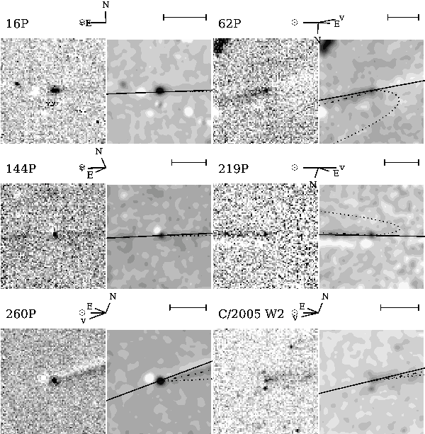
Figure 5: Same as Fig. 1, but for Spitzer/MIPS 24-µm images. Most images are background subtracted with the second (shadow) observation of the same comet. In these cases, the grayscale data limits are chosen to enhance the contrast of only one of the two comet images. Comets 16P/Brooks 2, 62P/Tsuchinshan 1, 144P/Kushida, 219P/2002 LZ₁₁ (LINEAR), 260P/2005 K3 (McNaught), and C/2005 W2 (Christensen) are shown.

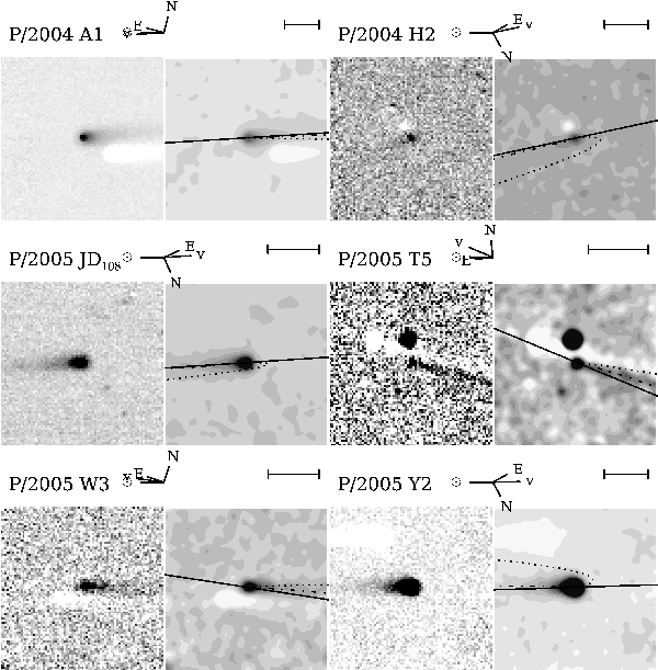
Figure 6: Same as Fig. 5, but for Comets P/2004 A1 (LONEOS), P/2004 H2 (Larsen), P/2005 JD₁₀₈ (Catalina-NEAT), P/2005 T5 (Broughton), P/2005 W3 (Kowalski), and P/2005 Y2 (McNaught).

3.2 Dust photometry

The Spitzer images allow us to estimate each comet’s dust mass and, for the IRS observations, color temperature. For comets with a coma and/or tail, we measure the total thermal emission in 3–6 pixel radius apertures centered on the comet. The smaller aperture sizes are necessary in some images to reduce background contamination. When possible, we also examine an aperture offset at least 5 pixels from the nucleus in order to measure emission from tails and trails. The size and shape of the tail/trail aperture varies comet-by-comet and depends on the morphology of the dust. The background is estimated from areas of low contamination from dust and background sources. As the thermal emission from comets typically contains significant emission from the nucleus, we only use the nucleus subtracted images from Paper I. The fluxes have been aperture corrected and color corrected assuming the spectral shape of an isothermal blackbody sphere in local thermodynamic equilibrium (LTE), according to the methods prescribed by the MIPS and IRS instrument handbooks (Colbert 2010, Spitzer Science Center 2009). The dust fluxes are listed in Table 2.

With the two IRS peak-up arrays, we measure the 16–22-µm color temperature of the dust in our survey, centered on the nucleus and in the tail/trail (if applicable) for all fluxes with signal-to-noise ratios $\geq 5$. Dust color temperatures are listed in Table 3 as a ratio with the temperature of an isothermal blackbody sphere in LTE at the same heliocentric distance ($T_{BB}=278\,r_{h}^{-1/2}$). The error-weighted mean of all color-temperature measurements is $\langle T/T_{BB}\rangle=1.074\pm 0.006$, of the center apertures is $1.079\pm 0.007$, and of the tail/trail apertures is $1.065\pm 0.010$.

The color temperature of the dust will only serve as an approximation to the true physical temperature of the grains because physical temperatures depend on the grain sizes, shapes, and compositions, and comet dust structures are collections of grains with a wide range of properties. For example, dust grains with sizes $\lesssim 1$ µm have higher equilibrium temperatures than larger grains because the former have smaller emission cross sections at 10–20 µm, the wavelength regime at which the peak of the thermal emission occurs for a blackbody sphere in the inner solar system. Thus, their equilibrium temperatures are increased over that of a blackbody. These increases are composition dependent as carbonaceous grains, which have high absorption and emission efficiencies, will have different equilibrium temperatures than an equally-sized silicate grain, which is less absorptive at most optical and infrared wavelengths. For more discussion on these effects, and how they may constrain thermal emission spectra, see Wooden (2002).

Despite the ambiguity in correlating color temperatures to coma grain properties, comet-to-comet differences indicate variations of those (unknown) dust parameters among the members of our survey. For example, the color temperature of 74P/Smirnova-Chernykh’s coma is greater than 101P-A/Chernykh’s coma ($1.16\pm 0.02$ versus $0.96\pm 0.03$, respectively). This difference indicates that 74P’s coma is composed of different grains than 101P’s coma, and we can speculate that they are smaller and/or more carbon rich in the former.

3.3 Survey sensitivity

3.3.1 All dust

The SEPPCoN survey was designed to detect comet nuclei with a signal-to-noise ratio of 30. The exposure times are not based on potential dust emission but solely on our estimated nucleus sizes and temperatures. To verify that we can draw meaningful results on the dust activity of Jupiter-family comets as a whole, we must estimate the survey’s sensitivity to dust. Rather than using a theoretical estimate (i.e., observation planning tools), we prefer to measure the sensitivities from our observations, which will easily take into account the effects of background objects (stars, asteroids, etc.), variances in instrument calibration (e.g., flat-fielding), latent charge on the detector, etc. To measure the sensitivity of an image, we first filter the image to remove structures larger than $5\times 5$ pixels (i.e., dust and the smoothly varying background). To be more specific, we applied a morphological gray closing operator, followed by the opening operator, and subtracted the result from the original image. The opening and closing operators effectively convolve the image with a $5\times 5$ box, but instead of replacing each pixel with the average of the surrounding pixels, the closing and opening operators replace each pixel with the maximum and minimum pixel values within the box, respectively. Applying the closing and opening operators is similar to applying a median filter, except more of the small scale structure is lost in median filtering. Because small scale structure affects our ability to detect dust, we prefer the closing and opening filters over the median. See Lea and Kellar (1989) and Appleton et al. (1993) for further discussion and other applications of morphological operators in astronomy. In the part of the co-added image where the integration time was the highest, we measure the standard deviation of the image after iteratively removing $3\sigma$ outliers (i.e., the comet itself, and the central cores of stars).

The image sensitivities are measured in units of MJy sr^-1. However, dust surface brightness depends on heliocentric distance: a surface brightness of 1 MJy sr^-1 at 3 AU implies less dust than 1 MJy sr^-1 at 7 AU due to the different equilibrium temperatures. A more relevant representation of the sensitivity is needed. We have chosen to transform the measured surface brightnesses into optical depths. To compute the image sensitivity to dust in terms of optical depth, we use the equation:

$$\sigma_{\tau}=\frac{\sigma_{I_{\nu}}}{C(T_{d})B_{\nu}(T_{d})\sqrt{A}},$$ (1)

where $\sigma_{\tau}$ is the optical depth (or effective fill factor) of a $1\sigma$ per pixel detection of dust, $\sigma_{I_{\nu}}$ is the measured sensitivity ($1\sigma$ per pixel) in units of MJy sr^-1, $T_{d}$ is the effective temperature of the dust, $C(T_{d})$ is the instrument color correction for a blackbody spectrum at a temperature $T_{d}$, $B_{\nu}(T_{d})$ is the Planck function evaluated at temperature $T_{d}$ in units of MJy sr^-1, and $A$ is the area of a fictitious dust aperture in units of square pixels. Our default aperture size in Table 2 is a 6 pixel radius circle. In §3.2, we computed a mean color temperature of $T_{c}/T_{BB}=1.08$ in the center aperture. A priori, we do not know the color temperature of any specific comet. Rather than using one value for 70 comets and our measured values for those 10 comets in Table 3, we assume $T_{d}\approx T_{c}=1.08\,T_{BB}=300\,r_{h}^{-1/2}$ K for all comets.

Histograms of the observed dust optical depths and the survey image sensitivities are presented in Fig. 7 for the IRS 22-µm and MIPS 24-µm observations. Notice that the dust detections fall off at the same optical depths as our estimated $3\sigma$ image sensitivities. This fall off strongly suggests our dust detections are sensitivity limited.

3.3.2 Trail dust

In a survey of 34 comets taken with the MIPS instrument, Reach et al. (2007) found that at least 80% of all short-period comets have dust trails. Since dust trails are long lived features (§3.1) we may expect a similar rate for the SEPPCoN targets, but instead we find a rate of 10%.

To better understand the dramatic difference in trail rates, we compared our survey target list to that in Reach et al. and found the following 12 comets in both surveys.

• Comet 107P did not have a trail, or any other dust, in any observation.

• Comet 62P had a trail in both surveys.

• Comet 78P’s dust was classified as a possible trail in SEPPCoN, and as having a trail by Reach et al..

• Comet 121P had a trail in SEPPCoN but only a tail in the Reach et al. survey. We suggest that this comet’s trail only becomes apparent at large true anomalies (trail survey $f=31\mbox{${}^{\circ}$}$, SEPPCoN $f=123\mbox{${}^{\circ}$}$).

• Comets 32P, 69P, 123P, and 131P had trails in the Reach et al. survey, but they appear to be too faint to detect in the SEPPCoN images. In particular, 123P’s SEPPCoN images have several nearby point sources and background subtraction artifacts (Fernández et al. 2011).

• Comets 48P and 129P had clear leading and following trails in the Reach et al. survey. The fields-of-view of the SEPPCoN observations are limited in the trailing direction and tails overlap with the orbit. It is surprising that the leading trails are not observed in either case. The leading trail may be a transient feature.

• Comets 94P and 127P were classified as an “intermediate trail” by Reach et al., i.e., the dust more closely followed the $\beta=10^{-3}$ syndyne than the projected orbit of the comet (this label is consistent with our “trail” label). Neither of these comets have dust in our survey images and both were taken at larger true anomalies, emphasizing that such dust may be relatively short lived (trail survey $f=62\mbox{${}^{\circ}$}$ and 77^∘, SEPPCoN $f=150\mbox{${}^{\circ}$}$ and -152^∘).

In summary, out of the 12 comets in both surveys, three morphologies have consistent descriptions (62P, 78P, and 107P), four trails appear to be too faint for SEPPCoN (32P, 69P, 123P, and 131P), two intermediate trails appear to be short lived and limited to smaller true anomalies (94P and 127P), one comet’s trail may not be present at very small true anomalies (121P), and two trails may be obfuscated by dust tails, whereas their leading trails are possibly transient features (48P and 129P). From this comet-by-comet comparison, it appears the low trail detection rate of SEPPCoN can be explained by: 1) observation timing/geometry; 2) the limited field-of-view of the IRS peak-up arrays; and, 3) the survey’s sensitivity to dust. The last point is discussed further below.

A portion of the difference in trail detection rates is due to the typical observing geometries of short-period comets at $r_{h}\gtrsim 4$ AU, which cause tails and trails to overlap on the sky (e.g., compare 22P to 48P in Fig. 1). However, obfuscation from brighter coma and tail dust does not explain the lack of trails in the 56 images of apparently bare nuclei. Instead, we must consider the survey differences in sensitivity. First note that the Reach et al. survey targeted comets within 3.5 AU from the Sun, whereas the SEPPCoN observations were all at $r_{h}\geq 3.4$ AU. Also note that the trail survey integration times were shallow (either 42 or 140 s on source with MIPS) compared to the SEPPCoN observations (140 to 2500 s with MIPS). We can make direct comparisons between the surveys by converting trail fluxes into optical depths. We examined the peak $\tau$ values listed in Table 2 of Reach et al., and find the trails have $0.2\mbox{$\times 10^{-9}$}\leq\tau\leq 9\mbox{$\times 10^{-9}$}$ in the mid-IR, with a median of 1.2$\times 10^{-9}$. For the eight SEPPCoN targets with trail detections, we find $0.4\mbox{$\times 10^{-9}$}\leq\tau\leq 11\mbox{$\times 10^{-9}$}$, and a median of 1.3$\times 10^{-9}$. In Fig. 7, we also show a histogram of the peak optical depths from the Reach et al. survey. The range and median trail optical depths of the two surveys roughly agree. But the Reach et al. trail survey did detect most of the faintest trails, and this is likely the main difference between the two surveys.

Figure 7: Histograms of the IRS 22-µm and MIPS 24-µm center (top panel) and tail/trail (upper-middle panel) photometry expressed as dust optical depth. Also shown are dust sensitivities ($3\sigma$ per 6-pixel radius aperture) in terms of optical depth for all IRS 22-µm and MIPS 24-µm images (lower-middle panel) and Spitzer trail survey peak optical depths (bottom panel) from Table 2 of Reach et al. (2007).

4 Discussion

4.1 Comet activity

Comet activity is controlled by physical and dynamical processes at the nucleus. Physical properties, such as composition and geology, determine if a comet is active under a given set of solar illumination conditions. Besides size and color temperature, little is known about the physical properties of our targets. The dynamical properties of a nucleus are described by its orbit and rotation state, and together they also determine the solar illumination conditions and history. The rotation states are known for only a few of our targets. In contrast, all of the orbital parameters are constrained well enough to make meaningful comparisons. The geometrical circumstances of each observation are also well constrained and can be tested. For example, we might test for a correlation between activity and observer-comet distance because dust around comets farther from the telescope is more difficult to detect (lower spatial resolution, possibly cooler dust temperatures).

For this work we have tested for the presence of a correlation between recent activity and eight observational and orbital parameters: $r_{h}$, $\Delta_{S}$ (Spitzer-comet distance), $\phi_{S}$ (phase angle, Sun-comet-Spitzer), $f$ (true anomaly), $q$ (perihelion distance), $e$ (orbital eccentricity), $a$ (orbital semi-major axis), and $\Delta q|_{150}$ (perihelion distance history, described below). All orbital parameters are measured from their osculating elements at the time of the observation, except $\Delta q|_{150}$. We integrated each comet’s current orbit back 300 yr in 90 day steps using HORIZONS (Giorgini et al. 1996); $\Delta q|_{150}$ is the difference between the minimum and maximum $q$ over the past 150 yr,

$$\Delta q=\mbox{min}(q)-\mbox{max}(q)$$ (2)

where a negative $\Delta q|_{150}$ indicates the perihelion distance was larger in the past. A relationship between any one of the above parameters and activity is not necessarily expected (e.g., we don’t expect activity to depend on the phase angle of the observation), but we tested for correlations in order to perform an unbiased study while getting a useful sense of what a “null hypothesis” result looks like.

For each parameter, we compute a two-sided Kolmogorov-Smirnov (K-S) statistic, $D$, and two-tailed $p$-value with the null hypothesis that the active and inactive comets in our survey are drawn from the same distribution. The $p$-value (or false positive probability) indicates the probability that uncorrelated data sets might result yield a $D$ greater than that observed. When $D$ is small, or when the $p$-value is large, the null hypothesis cannot be rejected. At first, only those comets with comae and/or tails were considered to be active. Comets with trails, or without dust are considered inactive. The four comets with ambiguous morphologies (tail/trail) are dropped from the analysis. With these definitions, the numbers of active and inactive comets are 21 and 64. Our K-S test results are listed in Table 4.

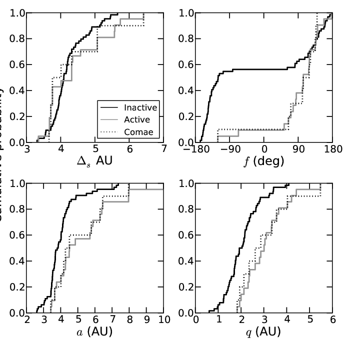
Figure 8: Cumulative probability functions comparing the distributions of Spitzer-comet distance ($\Delta_{S}$), true anomaly ($f$), orbital semi-major axis ($a$), and perihelion distance ($q$) for active (coma and/or tail) and inactive comets in our survey. The active distributions based solely on the presence of a coma are also shown.

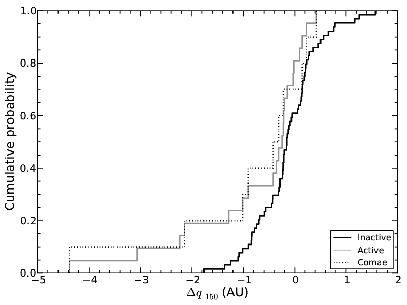
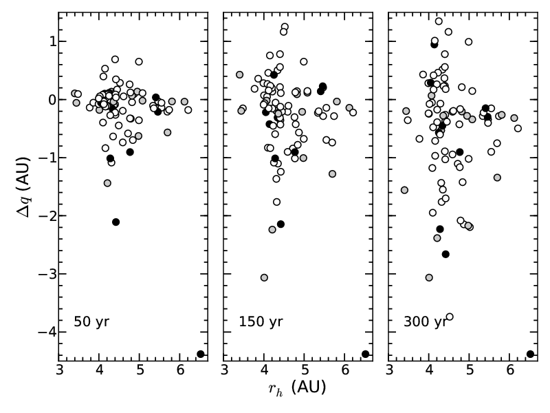
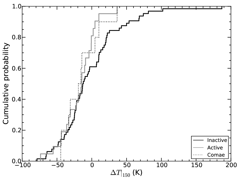
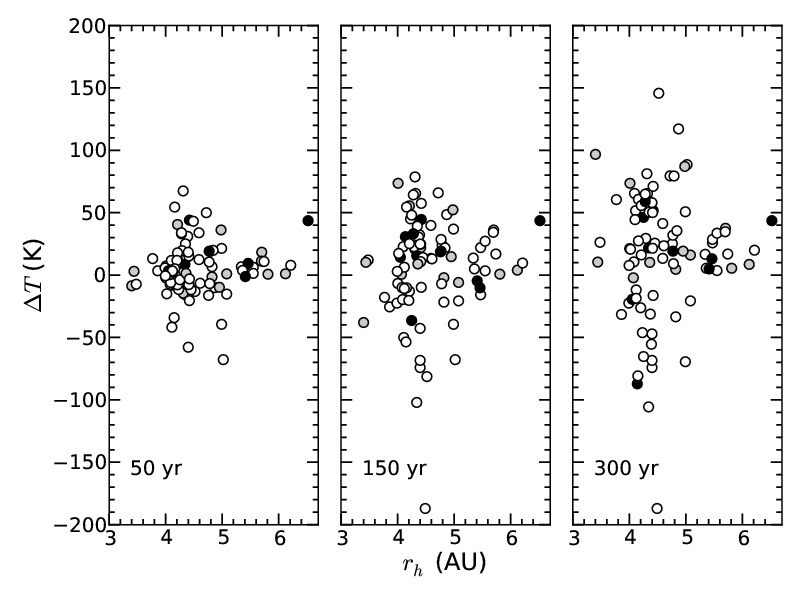
Figure 9: (Top left) Cumulative probability functions comparing the distributions of perihelion distance variations in the past 150 yr ($\Delta q|_{150}$) for active and inactive comets in our survey. (Top right) Plot of $\Delta q$ versus observed $r_{h}$ computed for 50-, 150-, and 300-yr orbital histories (comae: black, tails: gray, inactive: white). (Bottom left) Cumulative probability functions for peak-sub-solar-temperature variations in the past 150 yr ($\Delta T|_{150}$). (Bottom right) Plot of $\Delta T$ versus observed $r_{h}$ computed for 50-, 150-, and 300-yr orbital histories.

In §3.1, we argue that dust tails are associated with activity on longer timescales than dust comae, and that they do not necessarily indicate a currently active comet. As an additional check on the significance of our K-S tests, we removed tail-only detections from our active comet list, and compared the remaining comets to the inactive comets. This change reduced the number of active comets to 10. The second set of K-S tests are also presented in Table 4.

The $p$-values in Table 4 indicate that the active and inactive comets have significantly different $f$, $q$, $e$, and $a$ distributions. The distribution of $\Delta_{S}$ is slightly different but with less confidence, indicating that comet-Spitzer distance does not have a strong influence on our results. Figure 8 presents the cumulative probability functions for $f$, $q$, $a$, and $\Delta_{S}$. The cumulative probability functions for $\Delta q|_{150}$ are presented in Fig. 9. We discuss each result below.

4.1.1 True anomaly

The active and inactive comets have significantly different distributions in true anomaly. In Fig. 8, we see that the active comets are strongly biased toward positive true anomalies (i.e., post-perihelion), with only 2 active comets at $f<0$^∘ (i.e., pre-perihelion). Restricting our definition of active to only those comets with a coma does not diminish our conclusion. In addition, no comet in our survey is active between $f=-180$^∘ and $-125$^∘.

As an alternative metric of post-perihelion activity, we estimate the true anomalies at which activity starts and stops. Figure 10 shows a histogram of activity versus true anomaly, with a horizontal line plotted at $\exp(-1)$. We chose $\exp(-1)$ because it marks the half length of an exponential fall-off, however we note that our histogram does not necessarily suggest this particular functional relationship between activity and true anomaly. By comparing the line to the histogram, we estimate that activity in the average JFC turns on at $f>-120\mbox{${}^{\circ}$}$ and turns off at $f\approx 140\mbox{${}^{\circ}$}$.

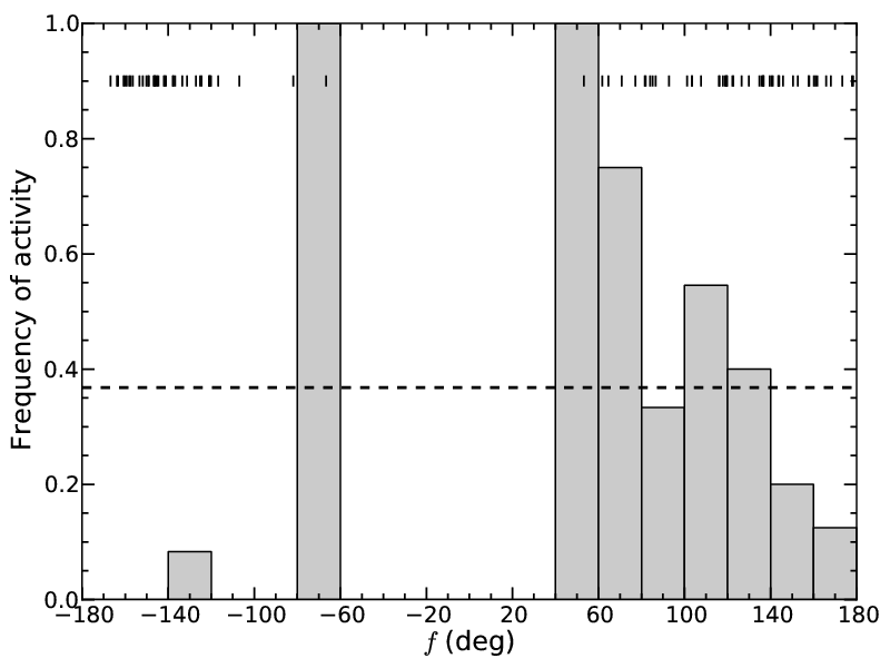
Figure 10: Frequency of activity versus true anomaly. A horizontal line is plotted at $e^{-1}$ in order to estimate at which true anomalies activity is typically initiated and quenched. Short vertical lines mark the true anomalies of individual targets.

A few scenarios may result in apparent persistent post-perihelion activity: 1) a temporary dust mantle insulates the ices during the pre-perihelion portion of the orbit but is lost near perihelion allowing persistent activity on the outbound leg of the orbit; 2) the surface layers retain a significant seasonal thermal wave that continues to heat the comet sub-surface when insolation would normally be insufficient; 3) a seasonal effect near perihelion that causes persistent activity well outside of perihelion; or, 4) asymmetric activity caused by the late onset of volatile production. For the purposes of this paper, we define a dust mantle to be an ice-free layer at the surface of the nucleus.

As solar insolation warms the surface of a comet a thermal wave propagates inward. At some depth the thermal wave heats ices to sublimation temperatures, which drives mass loss. The depth of those ices, the thermal properties of the layers above them, and the rotational and orbital states of the nucleus will determine when activity is initiated. Suppose that activity becomes so vigorous that any putative dust mantle is ejected, either partially or completely, from the comet. As the comet recedes from the Sun, activity would be stronger than the pre-perihelion orbit, but it would eventually decrease to the point at which it can no longer lift some grains from the surface, perhaps because of their large sizes, and a dust mantle will redevelop. Thus, a pre-perihelion nucleus could be insulated by a dust mantle, whereas the post-perihelion nucleus might not. Brin and Mendis (1979) present one of the first 1-D models of comet mantle formation and destruction that causes pre- and post-perihelion asymmetries near $r_{h}=1$ AU. Mantle formation and destruction in nucleus thermal models is reviewed by Prialnik et al. (2004).

In the second scenario, where activity is driven by seasonal heating, the dust mantle is not lost but retains heat from the perihelion passage. Energy deposited on diurnal timescales will radiate back to space on roughly the same timescale, but sub-surface temperatures can build up on longer timescales as a comet approaches perihelion. After the comet passes perihelion, the thermal wave cools to both space and the comet sub-surface. If sub-surface ices continue to be warmed to sublimation temperatures, despite the increasing heliocentric distance, activity will persist. In order to observe a pre-/post-perihelion asymmetry, the ices must be buried at depths closer to the annual thermal skin depth than the diurnal thermal skin depth. If this is true, gas production should not vary diurnally at the intermediate heliocentric distances in our survey, or, at least, it should be weakly correlated with rotational insolation. There is limited support for this scenario in flyby images of nuclei. Jet activity occurs from surfaces in local night at 81P/Wild 2, 9P/Tempel 1, and 103P/Hartley 2 (Sekanina et al. 2004, Farnham et al. 2007, A’Hearn et al. 2011), but the apparent timescales of this activity are much shorter than what is required for a pre-/post-perihelion asymmetry.

The near-surface structure of comets was directly examined by the Deep Impact mission (A’Hearn et al. 2005). Deep Impact excavated a crater with a diameter of 50–200 m on Comet 9P/Tempel 1 (Richardson and Melosh 2013, Schultz et al. 2013). According to A’Hearn (2008), most observations of the ejecta are consistent with dust-to-volatile ratios of order unity, and Groussin et al. (2010) came to the same conclusion. Since the dust-to-volatile ratio is not $\gg 1$, it appears the thermal wave in this nucleus had not sublimated much of the water ice on the scale of the crater depth. Even greater constraints on the depth of thermal penetration were obtained with Deep Impact spectra of the comet’s surface. Groussin et al. (2007) analyzed the thermal emission from the surface and showed that it has a low thermal inertia, nearly in instantaneous equilibrium with sunlight. They argue that cometary activity must originate within the first centimeters to meters of the surface. From the thermal inertia upper-limits and assumptions on conductivity and heat capacity, A’Hearn (2008) computes the diurnal skin depth to be 3 cm, and the annual skin depth to be 90 cm. These numbers are order of magnitude consistent with theoretical models of comet nuclei made before the Deep Impact mission results (Prialnik et al. 2004), and with Spitzer mid-IR spectral measurements of the nucleus thermal emission at 5 AU (Lisse et al. 2005). In order for dust mantles to quench activity on diurnal timescales, they must be larger than $\sim 1$ cm thick, and to prevent the seasonal thermal wave from driving activity, volatiles must be more than $\sim 10$ cm from the surface.

Weissman (1987) proposed that the sudden illumination of a nucleus hemisphere caused by the rapid change of season near perihelion causes cracks in the mantle, and these cracks create new active areas on the nucleus. The hemisphere illuminated on the in-bound leg of the orbit does not develop these cracks because it is gradually heated, and the surface can better accommodate the changes. If this hemisphere continues to be illuminated as the comet recedes from the Sun, the comet’s activity could be greater than that of it’s inbound leg.

Meech et al. (2011) propose that the pre-/post-perihelion asymmetry of Comet 103P/Hartley 2 is caused by the late on-set of CO₂ driven activity. They find that this comet’s activity was first initiated in 2010 at 4.3 AU by water sublimation. When the comet reached 1.4 AU (pre-perihelion) CO₂ driven activity dominated, to the point at which water ice can be driven off the surface, as if it were dust. The CO₂ driven activity would persist beyond the comet’s aphelion (Meech et al. 2011).

Whatever the cause, the effect is clear in the SEPPCoN. Because the survey took a consistent approach to its observations, it can be used to test these and other inhibitors and drivers of activity in a statistical manner.

4.1.2 Perihelion distance

The inactive comets have smaller perihelion distances than the active comets. The median $q$ is 2.0 AU for the inactive comets and 3.0 AU for the active comets. This difference may be a selection effect. Cometary activity is driven by insolation, and, in general, comets are most likely to be active when they are near perihelion. Our survey targets were observed at heliocentric distances ranging from 3 to 7 AU. However, a comet with a perihelion distance between 3 and 7 AU is a priori more likely to be active in our survey, since its activity at such distances has already been established (otherwise it would not have been designated a comet, and not observed by SEPPCoN). Therefore, the greater rate of activity for comets with larger perihelion distances appears to partially be an artifact of the survey.

To further demonstrate the larger activity rates of the large perihelia comets, we plot the cumulative frequency of activity in our survey, sorted by perihelion distance, in Fig. 11. That the frequency of activity almost continuously increases for $q>2$ AU shows the higher activity rate of this population.

Figure 12 presents an alternative view on these large perihelia comets, and shows that on average they produce more dust than the smaller perihelia comets. Here, we plot $\epsilon f\rho$ versus perihelion distance. We define the parameter $\epsilon f\rho$ as the product of effective emissivity ($\epsilon$), filling factor ($f$), and projected aperture radius ($\rho$, in units of cm). This parameter is intended to be analogous to the $Af\rho$ parameter commonly computed for scattered light observations (A’Hearn et al. 1984). Further discussion of $\epsilon f\rho$ can be found in A. We based our $\epsilon f\rho$ values on the mean MIPS 24-µm, or the IRS 22-µm center aperture photometry (Table 5). Comets with small $\epsilon f\rho$ values, i.e., low-activity comets, are missing from the large-perihelion population. We suggest that this bias is due to the discovery circumstances of large-perihelia comets, and that low-activity comets with large-perihelia are as yet missing from the discovered JFC population.

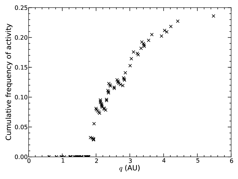
Figure 11: The cumulative frequency of activity in our survey versus perihelion distance.

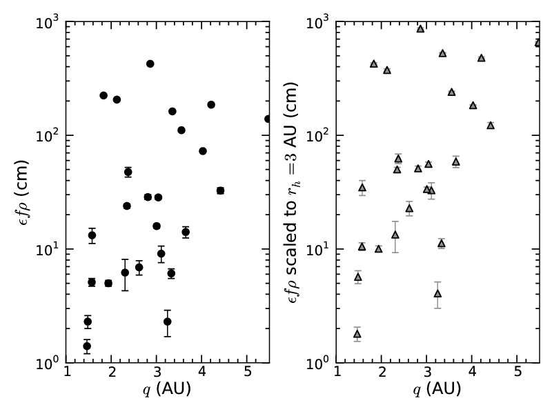
Figure 12: (Left) Comet activity, quantified with the parameter $\epsilon f\rho$, versus perihelion distance. (Right) The same as on the left, but $\epsilon f\rho$ has been scaled by $(r_{h}/3~{}{\rm AU})^{2}$, so that comets can be more directly compared to each other. Note the paucity of low-$\epsilon f\rho$ comets with large perihelion distances, indicating that our survey and the discovered JFC population is sensitivity limited.

Although we cannot make definite conclusions on the activity of comets with large-perihelia, we can consider the activity of small-perihelia comets, whose discovery rates are likely more complete and less biased. Of those comets with $q<2.5$ AU, 7 out of 59 comets (12%) are active, and none of the 30 comets with $q<1.8$ AU are active (Fig. 11). Therefore any short-period comet with a small perihelion distance is likely inactive at 3–7 AU. This finding may be explained if relatively more volatile ices are lost for comets that approach the Sun more closely during their perihelion passages, but this hypothesis seems inconsistent with the results of A’Hearn et al. (2012). They studied the H₂O, CO₂, and CO content of comets in the literature, and found no correlation with orbital parameters, except for a decreasing CO₂-to-H₂O mixing ratio for comets with decreasing perihelion distance, for $q<1$ AU. They rightly dismiss this correlation as due to small number statistics (only 4 comets have a measured CO₂ abundance for $q<1$ AU) and for the fact that it contradicts their result that CO/H₂O is uncorrelated with $q$. Taking our results together with the discussion of A’Hearn et al. (2012), we suggest that comets with small perihelion distances have a thicker insulating surface than comets with larger perihelion distances.

4.1.3 Perihelion distance history

Licandro et al. (2000) surveyed 18 comets in order to estimate the effective sizes of their nuclei. Seven of their targets were active: one at $r_{h}=3.04$ AU, and the rest at $r_{h}>4$ AU. They examined their orbital histories and found that all but one of their comets recently perturbed to orbits with smaller perihelion distances in the past 150 yr ($\Delta q|_{150}<-1$ AU) were active. Licandro et al. hypothesize that the perturbations to smaller perihelion distances caused a marginally stable mantle to be destroyed, exposing fresh ices. The absence of a mantle allows activity to persist to larger than usual perihelion distances. When we examined the pre-/post-perihelion asymmetry in SEPPCoN, we also introduced the concept of a temporary mantle, only in our case the mantle is partially or completely lost each perihelion passage. We now examine the orbital histories of SEPPCoN targets to further investigate the potential existence of dust mantles. Note that a small $\Delta q$ is not the same as small $q$, i.e., a comet may be perturbed from the Centaur region ($a>5.2$ AU) into the Jupiter-family comet region ($a<5.2$ AU), yielding $\Delta q<0$, yet still have a large perihelion distance in our survey.

Recognizing that the same $\Delta q$ is more significant at small perihelion distances than at large perihelion distances, we have also computed the maximum sub-solar-temperature difference, $\Delta T$. The sub-solar temperature of a spherical comet nucleus is

$$T=\left[\frac{(1-A)*F_{\odot}}{r_{h}^{2}\eta\epsilon\sigma_{SB}}\right]^{1/4},$$ (3)

where $A$ is the Bond albedo, $F_{\odot}=1365$ W m ^-2 is the solar constant at 1 AU, $r_{h}$ is the heliocentric distance in AU, $\eta=1.03$ is the IR-beaming parameter, $\epsilon=0.95$ is the IR emissivity of the surface, and $\sigma_{SB}$ is the Stefan-Boltzmann constant in W m^-2 K^-4 (Harris 1998, Fernández et al. 2011). For our purposes, we compute $\Delta T|_{x}$ using the minimum and maximum $q$ values from our $\Delta q|_{x}$ integrations; $\Delta T>0$ signifies the temperature was cooler in the past.

Figure 9 shows that active comets in SEPPCoN appear more likely to have $\Delta q|_{150}<0$ and $\Delta T|_{150}>0$ than the inactive comets. In addition, no active comet has $\Delta q|_{150}>0.5$ AU, yet $\approx 10$% of the inactive comets do have such large values. The K-S probabilities for $\Delta q|_{150}$ and $\Delta T|_{150}$ are 28% and 10%, indicating that the difference between active and inactive comets may be significant. But, given the striking differences in Fig. 9, this problem deserves future study because it may lead to an understanding of the timescales of mantle formation.

The difference in perihelion distance histories between the active and inactive comets may be related to their discovery circumstances. When an unknown comet is perturbed to a smaller perihelion distance, it should become brighter to observers on the Earth, and therefore more likely to be discovered. To investigate this possible effect, we searched the NASA JPL Small-Body Database Browser and the NASA Planetary Data System Small Bodies Node for each comet’s year of discovery. We plot this year versus the year of the minimum $\Delta q|_{150}$ in Fig. 13. Data points near a slope of 1 indicate a comet that was discovered at a 150-year low in its perihelion distance history. Fifteen comets are found within 20 years of this line, indicating that reductions in perihelion distance is a factor in JFC discovery dates. In the plot we indicate which comets were active in our survey. Those comets discovered soon after being scattered to smaller perihelion distances appear to have a higher activity rate in our survey, 8 out of 22 ($36\pm 13\%$) versus 15 out of 70 ($21\pm 6$%), but the low significance precludes us from making a firm conclusion.

Figure 13: Year of comet discovery ($T_{disc}$) versus the year of the comet’s 150-year minimum in perihelion distance history ($T_{\Delta q|_{150}}$). Comets between the dotted and solid trend lines are those that were discovered near a 150-year minimum in perihelion distance: 8 out of the 22 comets in this region are active in our survey.

Most of our survey targets were discovered in the past 20 years, but the year of minimum $\Delta q|_{150}$ for these comets is uniformly distributed over the past 150 years. This distribution may be the result of uncertain orbital histories for these comets, rather than a lack of correlation between the two parameters. However, it is also possible that the increasing sophistication and sensitivity of Solar System surveys in the past 20 years has led to JFC discoveries that are independent of their perihelion distance history. Both of these possibilities could be a cause for the low significance of the K-S tests based on $\Delta q$.

4.1.4 Semi-major axis and Spitzer-comet distance

On average, the active comets have larger semi-major axes than the inactive comets. Since perihelion distance and semi-major axis are correlated in the Jupiter-family comet population, this difference may be an observational bias related to the perihelion distance bias described above. A similar argument may be made for the slight differences in $\Delta_{S}$ for the active and inactive comets. Nuclei with larger $q$ are more likely to be observed at larger $\Delta_{S}$.

4.1.5 Other investigations

Comet lightcurve asymmetries have been recognized for many years. Asymmetries near perihelion are not directly relevant to our survey since most of our targets are observed at true anomalies greater than 90^∘ from perihelion. The secular light curves of 27 comets were studied by Ferrín (2010). Considering only the Jupiter-family comets, and excluding the one-time active Comet 107P/Wilson-Harrington (leaving 17 comets), the ratios of the heliocentric distance at which activity ceases ($r_{off}$) to the distance at which activity initiates ($r_{on}$) ranges from 0.7 to 2.0, with a mean $r_{off}/r_{on}=1.20\pm 0.38$. Although this result cannot be directly compared to our survey results, they qualitatively agree in that it appears persistent post-perihelion activity is common to individual Jupiter-family comets.

The activity of short-period comets has also been examined by Mazzotta Epifani et al. (2009). They searched the literature for optical and infrared observations of short-period comets (Jupiter-family, Encke type, and Halley type) at $r_{h}>3$ AU. In their compilation of 90 comets they find that 10–20% are active beyond 4.5 AU. Furthermore, they also find a perihelion asymmetry with activity detected in 22% of the pre-perihelion observations, and 59% of the post-perihelion observations. In our survey data ($r_{h}>3.4$) we find slightly different values: $24\pm 5$% (21 comets) of our sample was active, with activity in $5\pm 4$% (2/39) of the pre-perihelion observations, and $38\pm 9$% (19/50) in the post-perihelion observations. With only a few comets in each bin, and understanding that the Mazzotta Epifani et al. study is based on a literature search, and not on a consistent data set, we consider the SEPPCoN results to be compatible with the results of Mazzotta Epifani et al.. In addition, they also conclude that recent perihelion distance changes are not a strong predictor of distant activity, agreeing with our results above.

4.2 Dust color temperature

The effective temperatures of comet comae at 5–20 µm typically range from $\approx 0-30$% warmer than an isothermal blackbody sphere at the same heliocentric distance (Gehrz and Ney 1992, Lisse et al. 1998, Sitko et al. 2004, Woodward et al. 2011). In Table 3 we find a similar result, even though our observations are obtained at larger heliocentric distances and longer wavelengths than are typically measured with ground-based observatories.

We test for correlations between $T_{c}/T_{BB}$ for the 11 IRS center aperture measurements and the parameters $r_{h}$, $q$, $F_{22}$ (22- or 24-µm flux), and $\epsilon f\rho$. The results are presented in Table 5. For each parameter, we calculate the linear correlation coefficient and apply a Spearman “$\rho$” test. The Spearman test is a more robust estimate of correlation than the linear correlation coefficient. It is based on the relative rankings of each parameter being tested, and does not test for a specific functional form of the correlation. After computing the Spearman $\rho$, we derive $Z$, the number of standard deviations by which the Spearman statistic deviates from the null hypothesis expectation value for uncorrelated data. To account for measurement uncertainties in the correlation tests, we tested $10^{4}$ data sets generated with a Monte Carlo technique based on our measurements and associated uncertainties. No significant correlation is found, and the correlations in our Monte Carlo runs never exceeded a $3\sigma$ significance. We list our results in Table 6.

5 Conclusions

We presented an analysis of the dust and activity of comets observed by the Spitzer Space Telescope as part of the Survey of the Ensemble Physical Properties of Cometary Nuclei (SEPPCoN). We have shown that SEPPCoN can be used to study the dust and activity of Jupiter-family comets at 3–7 AU, although some care must be taken when interpreting the results as the dust detections are limited by the image sensitivities, and that comets with large perihelion distances are a priori more active. We detected dust around 33 of 89 ($37\pm 6$%) survey targets, and 21 targets ($24\pm 5$%) have comae or tails that suggest recent cometary activity. Since faint dust ($\tau\lesssim 0.5\mbox{$\times 10^{-9}$}$) may remain undetected in our images, we conclude our detections are a lower limit and that at least $\approx 24$% of Jupiter-family comets are active at 3–7 AU from the Sun. We also studied the crude spectral properties of the dust. The 16- to 22-µm color temperature of the dust is $7.4\pm 0.6$% warmer on average than an isothermal blackbody sphere in LTE.

We introduce the quantity $\epsilon f\rho$, intended to be a thermal emission counterpart to the often reported $Af\rho$ for observations of light scattered by comets. The $\epsilon f\rho$ versus perihelion distance distribution of our survey sample shows that low-activity comets with large perihelion distances are missing from the survey, and therefore are likely missing from the known Jupiter-family comet population.

We compared the frequency of activity of survey targets to their orbital and observational parameters. All 30 comets with $q<1.8$ AU appear inactive in our survey. Whatever drives their activities is effectively quenched at larger distances from the Sun.

Comets that have been perturbed to smaller perihelion distances in the past 150 years seem more likely to be active in our survey (cf. Licandro et al. 2000). Kolmogorov-Smirnov tests indicate a tentative result, so a better statistical characterization, perhaps with more detailed orbital histories, is warranted.

The activity of Jupiter-family comets at 3–7 AU from the Sun is significantly biased to post-perihelion epochs. Of the 21 comets that appear to be recently active, 19 were observed post-perihelion. We tentatively estimate the true anomaly at which activity is initiated to be $f>-120$^∘, but small number statistics make this limit uncertain. With better confidence, we find that for many comets activity has ceased by $f\approx 140$^∘. Similar findings on the persistent post-perihelion activity were found by Mazzotta Epifani et al. (2009), and Ferrín (2010). No comet in our survey is active between $f=-180$^∘ and $-125$^∘.

We discussed several causes for a pre-/post-perihelion activity asymmetry. Whatever the cause, the effect is clear in our survey. Because SEPPCoN took a consistent approach to its observations, it can be used to test the drivers and inhibitors of activity in a statistical manner. The Rosetta spacecraft, which will orbit Comet 67P/Churyumov-Gerasimenko (Glassmeier et al. 2007) as it approaches perihelion from 4 AU, should also provide new perspectives on this problem of the evolutionary history of comet surfaces.

Table 1: SEPPCoN target list, observational geometry, and orbital parameters: Obs. date – Spitzer observation date, for MIPS observations, only one of the two epochs are listed; $r_{h}$ – heliocentric distance; $\Delta_{S}$ – Spitzer comet distance; $\phi_{S}$ – Sun-comet-Spitzer angle; $f$ – true anomaly, 0^∘ at perihelion; $T-T_{p}$ – time from perihelion, $<0$ when $f<0$; $a$ – semi-major axis; $e$ – eccentricity; $q$ – perihelion distance; $\Delta q|_{150}$ – change in $q$ over the past 150 yr.

Name	Obs. date	$r_{h}$	$\Delta_{S}$	$\phi_{S}$	$f$	$T-T_{p}$	$a$	$e$	$q$	$\Delta q|_{150}$
	(UT)	(AU)	(AU)	(∘)	(∘)	(days)	(AU)		(AU)	(AU)
6P/d’Arrest	2007-02-13 22:48	4.39	3.85	12	-145	-548	3.49	0.61	1.35	-0.23
7P/Pons-Winnecke	2007-04-19 14:39	4.34	4.03	13	-146	-526	3.43	0.63	1.25	0.50
11P/Tempel-Swift-LINEAR	2006-09-01 15:12	4.40	4.04	13	-146	-611	3.42	0.54	1.56	0.56
14P/Wolf	2007-03-20 17:52	4.52	4.53	13	-120	-709	4.25	0.36	2.72	1.25
15P/Finlay	2007-02-28 03:06	4.40	4.32	13	-149	-480	3.48	0.72	0.97	0.21
16P/Brooks 2	2007-04-10 09:32	3.40	3.37	17	-125	-368	3.36	0.56	1.47	0.43
22P/Kopff	2007-04-19 14:10	4.87	4.38	11	-156	-767	3.46	0.54	1.58	-0.57
31P/Schwassmann-Wachmann 2	2006-11-09 10:30	5.02	4.59	11	-167	-1423	4.23	0.19	3.42	1.57
32P/Comas Solà	2006-08-01 03:59	4.14	3.76	14	122	486	4.27	0.57	1.83	-0.42
33P/Daniel	2006-11-09 17:14	4.40	4.17	13	-127	-619	4.03	0.46	2.17	0.78
37P/Forbes	2007-03-12 00:56	4.31	4.19	13	144	587	3.43	0.54	1.57	-0.19
47P/Ashbrook-Jackson	2007-03-21 10:56	4.32	4.32	13	-117	-682	4.12	0.32	2.79	-1.76
48P/Johnson	2006-11-11 18:43	4.41	4.32	13	141	761	3.65	0.37	2.31	-0.35
50P/Arend	2006-10-23 18:43	3.48	3.31	17	-107	-373	4.09	0.53	1.92	-0.15
51P-A/Harrington	2007-04-06 23:24	3.77	3.35	15	-125	-438	3.70	0.55	1.68	0.19
56P/Slaughter-Burnham	2006-12-23 13:48	5.08	5.04	12	120	708	5.10	0.50	2.53	0.12
57P-A/du Toit-Neujmin-Delaporte	2007-06-15 08:34	4.11	3.92	14	-138	-560	3.45	0.50	1.72	0.46
62P/Tsuchinshan 1	2006-10-03 02:00	4.72	4.66	12	150	664	3.52	0.58	1.48	-0.84
68P/Klemola	2007-02-12 09:42	5.47	5.28	10	-138	-709	4.89	0.64	1.76	-0.29
69P/Taylor	2006-07-29 05:19	4.25	3.66	12	135	605	3.65	0.47	1.94	0.42
74P/Smirnova-Chernykh	2007-01-28 17:01	4.42	4.01	12	-121	-914	4.17	0.15	3.56	-2.14
77P/Longmore	2007-02-10 07:38	4.59	4.18	12	-152	-878	3.60	0.36	2.31	-0.90
78P/Gehrels 2	2007-03-10 02:00	4.98	4.46	10	153	865	3.74	0.46	2.01	-1.01
79P/du Toit-Hartley	2006-09-17 23:10	4.37	4.08	13	-158	-618	3.03	0.59	1.23	-0.22
89P/Russell 2	2007-05-01 09:31	4.76	4.18	11	-146	-839	3.80	0.40	2.28	-0.30
93P/Lovas 1	2006-10-03 23:46	4.01	3.56	14	-121	-439	4.39	0.61	1.71	0.07
94P/Russell 4	2006-11-14 19:47	4.79	4.20	11	178	1174	3.51	0.36	2.24	-0.43
101P-A/Chernykh	2007-04-22 13:51	4.34	3.76	12	103	483	5.78	0.59	2.35	-0.31
107P/Wilson-Harrington	2007-02-12 07:43	4.08	3.52	13	166	582	2.64	0.62	0.99	0.05
113P/Spitaler	2006-10-22 15:58	3.86	3.55	15	-120	-518	3.69	0.42	2.13	0.36
118P/Shoemaker-Levy 4	2006-09-17 11:45	4.95	4.58	12	178	1159	3.47	0.42	2.00	-0.21
119P/Parker-Hartley	2007-02-12 08:01	4.21	3.67	12	103	629	4.29	0.29	3.04	-2.24
121P/Shoemaker-Holt 2	2006-08-01 02:40	4.35	3.97	13	123	696	4.02	0.34	2.65	-1.10
123P/West-Hartley	2006-10-21 23:31	5.34	4.91	10	161	1049	3.86	0.45	2.13	-0.23
124P/Mrkos	2006-09-16 19:19	4.23	3.76	13	-149	-588	3.21	0.54	1.47	-0.45
127P/Holt-Olmstead	2007-03-08 16:37	4.59	4.43	13	-164	-957	3.44	0.37	2.18	-0.21
129P/Shoemaker-Levy 3	2007-04-19 00:39	4.01	3.67	14	119	679	3.76	0.25	2.81	-3.06
130P/McNaught-Hughes	2006-11-14 10:57	4.45	4.20	13	146	752	3.54	0.41	2.10	-0.21
131P/Mueller 2	2007-02-12 08:54	4.42	3.96	12	140	787	3.68	0.34	2.42	-1.24
132P/Helin-Roman-Alu 2	2007-06-07 19:26	3.99	3.80	15	120	478	4.09	0.53	1.92	0.28
137P/Shoemaker-Levy 2	2007-03-16 13:11	5.47	5.45	11	-142	-788	4.48	0.58	1.89	0.21
138P/Shoemaker-Levy 7	2007-01-22 19:49	4.21	4.21	14	136	552	3.63	0.53	1.71	0.14
139P/Väisälä-Oterma	2006-11-02 07:11	4.10	3.57	13	-82	-535	4.51	0.25	3.40	-0.83
143P/Kowal-Mrkos	2007-03-09 16:14	4.99	4.74	11	-133	-825	4.30	0.41	2.54	0.65
144P/Kushida	2007-07-09 22:38	4.61	4.16	12	-142	-567	3.86	0.63	1.44	-0.11
146P/Shoemaker-LINEAR	2006-08-06 20:20	5.08	4.86	12	-147	-649	4.03	0.66	1.39	0.15
148P/Anderson-LINEAR	2006-11-02 10:30	4.31	3.89	13	-137	-567	3.68	0.54	1.70	-1.36
149P/Mueller 4	2007-02-09 03:36	5.55	5.46	10	-150	-1106	4.33	0.39	2.65	-0.70
152P/Helin-Lawrence	2006-09-17 20:19	5.70	5.58	10	158	1364	4.50	0.31	3.11	-1.28
159P/LONEOS	2007-02-13 08:58	6.12	5.74	9	118	1078	5.88	0.38	3.65	-0.14
160P/LINEAR	2006-12-19 16:49	4.99	4.83	12	144	798	3.98	0.48	2.08	-0.68
162P/Siding Spring	2007-03-17 23:43	4.82	4.27	11	173	858	3.05	0.60	1.23	0.14
163P/NEAT	2006-08-06 17:59	4.09	3.95	14	130	552	3.67	0.48	1.92	0.27
168P/Hergenrother	2007-05-23 02:26	4.49	4.09	12	144	567	3.63	0.61	1.42	1.17
169P/NEAT	2007-03-01 18:40	4.29	4.01	13	168	530	2.60	0.77	0.61	-0.05
171P/Spahr	2007-03-16 13:00	4.16	4.09	14	137	559	3.53	0.51	1.73	-0.84
172P/Yeung	2006-10-18 20:36	4.25	4.06	14	-141	-725	3.51	0.36	2.24	-1.09
173P/Mueller 5	2006-10-24 09:18	4.82	4.32	11	-67	-572	5.71	0.26	4.21	0.09
197P/LINEAR	2006-11-04 17:12	4.21	4.02	14	-159	-561	2.87	0.63	1.06	-0.15
213P/2005 R2 (Van Ness)	2006-11-13 12:57	4.05	3.71	14	137	641	3.43	0.38	2.13	-0.22
215P/2002 O8 (NEAT)	2007-01-08 17:45	4.77	4.24	11	-161	-1245	4.03	0.20	3.22	-1.01
216P/2001 CV8 (LINEAR)	2007-01-01 12:48	4.41	3.95	12	-131	-648	3.89	0.44	2.16	-0.43
219P/2002 LZ11 (LINEAR)	2007-06-07 04:31	4.78	4.22	11	-160	-1004	3.65	0.35	2.37	0.12
221P/2002 JN16 (LINEAR)	2007-04-10 02:54	4.40	3.83	12	-145	-656	3.48	0.49	1.79	-0.31
223P/2002 S1 (Skiff)	2007-04-06 00:18	5.70	5.15	9	-163	-1229	4.14	0.42	2.41	-0.74
228P/2001 YX127 (LINEAR)	2006-10-22 11:26	4.84	4.44	12	162	1330	4.16	0.18	3.43	-0.78
246P/2004 F3 (NEAT)	2006-12-17 23:20	4.28	3.71	12	119	712	4.02	0.29	2.87	-1.01
256P/2003 HT15 (LINEAR)	2006-12-06 12:30	6.21	5.66	-8	158	1328	4.61	0.42	2.68	-0.22
260P/2005 K3 (McNaught)	2007-01-01 07:44	4.20	3.94	14	136	508	3.69	0.59	1.51	0.20
C/2005 W2 (Christensen)	2007-01-01 04:24	4.07	3.76	14	53	280	18.93	0.82	3.33	-0.02
P/2001 R6 (LINEAR-Skiff)	2007-04-05 14:06	5.74	5.18	9	-158	-1086	4.15	0.48	2.17	-0.29
P/2003 O3 (LINEAR)	2007-07-09 12:00	4.28	4.10	14	-153	-571	3.10	0.60	1.25	-0.60
P/2004 A1 (LONEOS)	2007-03-05 01:21	6.52	6.42	9	71	910	7.96	0.31	5.48	-4.38
P/2004 DO29 (Spacewatch-LINEAR)	2006-09-18 04:24	5.55	5.21	10	82	712	7.36	0.44	4.09	-0.14
P/2004 H2 (Larsen)	2007-01-01 20:40	5.46	5.07	10	140	965	4.51	0.42	2.62	0.23
P/2004 V3 (Siding Spring)	2006-09-18 05:33	5.36	4.90	10	82	676	7.12	0.45	3.94	-0.20
P/2004 V5-A (LINEAR-Hill)	2007-03-10 01:13	5.81	5.57	10	77	737	7.98	0.45	4.42	-0.03
P/2004 VR8 (LONEOS)	2006-08-07 18:51	3.44	3.35	17	85	339	4.86	0.51	2.38	-0.19
P/2005 GF8 (LONEOS)	2006-11-12 23:27	4.16	3.79	14	87	452	5.85	0.52	2.83	0.24
P/2005 JD108 (Catalina-NEAT)	2007-01-01 21:20	4.77	4.32	11	65	509	6.45	0.38	4.03	-0.90
P/2005 JQ5 (Catalina)	2006-11-21 13:58	4.02	4.00	15	160	482	2.69	0.69	0.83	-0.06
P/2005 L4 (Christensen)	2007-03-11 23:02	4.15	4.07	14	116	564	4.12	0.43	2.37	0.76
P/2005 Q4 (LINEAR)	2007-02-28 09:05	4.41	3.93	12	127	518	4.46	0.61	1.75	-0.12
P/2005 R1 (NEAT)	2006-12-19 12:41	4.12	3.72	14	108	-276	5.50	0.63	2.05	0.16
P/2005 S3 (Read)	2007-05-23 02:48	4.12	3.88	14	93	500	4.90	0.42	2.84	-0.15
P/2005 T5 (Broughton)	2006-10-09 13:43	3.99	3.71	15	62	340	7.26	0.55	3.25	-0.09
P/2005 W3 (Kowalski)	2006-12-08 04:36	4.36	4.35	13	84	472	6.40	0.53	3.01	-0.24
P/2005 XA54 (LONEOS-Hill)	2007-06-04 23:12	4.42	3.86	12	116	454	6.13	0.71	1.77	0.11
P/2005 Y2 (McNaught)	2007-01-20 05:02	5.41	5.07	10	101	753	6.30	0.47	3.36	0.14

Table 1: continued

Table 2: Dust morphology and photometry. Table columns: Instrument – the name of the instrument used; Morph. – Morphology “N” for no dust detected, “C” for coma, “Ta” for tail, “Tr” for trail, a “?” indicates a tentative detection of dust; $\rho$ – the radius of the circular aperture centered on the comet nucleus; For MIPS, $F_{1}$ and $F_{2}$ are the flux densities of the two 23.7-µm observations; For IRS, $F_{1}$ and $F_{2}$ are the flux desnities of the 15.8-µm and 22.3-µm peak up arrays; $d$ – The distance of the tail/trail aperture from the center of the comet nucleus; $A$ – The area of the aperture used to measure the tail/trail flux.

			Center aperture					Tail or trail aperture
Comet	Instru-	Morph.	$\rho$	$F_{1}$	$\sigma_{1}$	$F_{2}$	$\sigma_{2}$	$d$	$A$	$F_{1}$	$\sigma_{1}$	$F_{2}$	$\sigma_{2}$
	ment		(px)	(mJy)		(mJy)		(px)	(px)	(mJy)		(mJy)
6P/d’Arrest	IRS	Tr?	6	$\cdots$	$\cdots$	$\cdots$	$\cdots$	$\cdots$	$\cdots$	$\cdots$	$\cdots$	$\cdots$	$\cdots$
16P/Brooks 2	MIPS	Ta/Tr	6	0.528	0.062	$\cdots$	$\cdots$	5	16.9	0.180	0.023	$\cdots$	$\cdots$
22P/Kopff	IRS	Tr	6	0.726	0.075	1.16	0.17	11	91.8	1.109	0.067	2.53	0.16
32P/Comas Solà	IRS	C+Ta	6	16.21	0.27	33.10	0.55	5	138.9	8.21	0.30	19.15	0.62
37P/Forbes	IRS	Ta/Tr	6	$\cdots$	$\cdots$	0.625	0.051	7	58.3	0.205	0.028	0.536	0.036
48P/Johnson	IRS	Ta	6	0.61	0.16	0.69	0.21	12	47.9	0.63	0.10	0.99	0.13
50P/Arend	IRS	Ta?	$\cdots$	$\cdots$	$\cdots$	$\cdots$	$\cdots$	$\cdots$	$\cdots$	$\cdots$	$\cdots$	$\cdots$	$\cdots$
56P/Slaughter-Burnham	IRS	Ta/Tr	3	$\cdots$	$\cdots$	$\cdots$	$\cdots$	15	77.2	0.216	0.027	0.315	0.058
62P/Tsuchinshan 1	MIPS	Tr	4	0.177	0.034	0.242	0.050	12	72.0	0.377	0.040	$\cdots$	$\cdots$
69P/Taylor	IRS	C	4	$\cdots$	$\cdots$	0.477	0.031	$\cdots$	$\cdots$	$\cdots$	$\cdots$	$\cdots$	$\cdots$
74P/Smirnova-Chernykh	IRS	C+Tr	6	6.52	0.19	13.30	0.19	14	104.2	1.55	0.18	3.28	0.18
78P/Gehrels 2	IRS	Ta/Tr	$\cdots$	$\cdots$	$\cdots$	$\cdots$	$\cdots$	13	59.8	0.320	0.035	0.804	0.084
101P-A/Chernykh	IRS	C	6	1.136	0.060	3.20	0.13	$\cdots$	$\cdots$	$\cdots$	$\cdots$	$\cdots$	$\cdots$
118P/Shoemaker-Levy 4	IRS	Ta	6	0.248	0.074	$\cdots$	$\cdots$	6	64.9	$\cdots$	$\cdots$	0.405	0.085
119P/Parker-Hartley	IRS	Ta	6	1.81	0.10	4.16	0.18	12	88.0	1.914	0.088	4.27	0.14
121P/Shoemaker-Holt 2	IRS	Tr	$\cdots$	$\cdots$	$\cdots$	$\cdots$	$\cdots$	13	148.4	2.33	0.13	4.98	0.23
129P/Shoemaker-Levy 3	IRS	Ta	6	$\cdots$	$\cdots$	4.65	0.23	7	43.6	$\cdots$	$\cdots$	3.05	0.14
144P/Kushida	MIPS	Tr	6	$\cdots$	$\cdots$	$\cdots$	$\cdots$	27	142.2	$\cdots$	$\cdots$	0.61	0.18
152P/Helin-Lawrence	IRS	Ta	6	$\cdots$	$\cdots$	0.427	0.072	12	57.4	0.321	0.038	0.818	0.050
159P/LONEOS	IRS	Ta	6	0.315	0.036	0.539	0.060	15	57.6	0.259	0.025	0.891	0.042
171P/Spahr	IRS	Tr	$\cdots$	$\cdots$	$\cdots$	$\cdots$	$\cdots$	15	50.2	0.285	0.030	0.293	0.038
173P/Mueller 5	IRS	Ta	6	6.75	0.26	16.96	0.27	15	111.9	4.65	0.26	13.03	0.27
213P/2005 R2 (Van Ness)	IRS	C+Ta	6	14.96	0.39	32.35	0.74	14	224.7	21.82	0.57	45.6	1.1
219P/2002 LZ11 (LINEAR)	MIPS	Tr	4	$\cdots$	$\cdots$	$\cdots$	$\cdots$	37	217.9	1.01	0.11	0.98	0.10
246P/2004 F3 (NEAT)	IRS	C+Ta	6	25.57	0.48	59.2	1.1	11	327.5	36.33	0.88	87.6	2.0
260P/2005 K3 (McNaught)	MIPS	Tr	$\cdots$	$\cdots$	$\cdots$	$\cdots$	$\cdots$	38	402.2	2.33	0.12	$\cdots$	$\cdots$
C/2005 W2 (Christensen)	MIPS	Ta	6	$\cdots$	$\cdots$	1.41	0.14	24	163.9	2.04	0.18	2.68	0.17
P/2004 A1 (LONEOS)	MIPS	C+Ta	6	6.65	0.14	6.10	0.11	21	217.9	6.55	0.20	5.98	0.16
P/2004 H2 (Larsen)	MIPS	C	4	0.415	0.062	$\cdots$	$\cdots$	$\cdots$	$\cdots$	$\cdots$	$\cdots$	$\cdots$	$\cdots$
P/2004 V5-A (LINEAR-Hill)	IRS	Ta	6	0.640	0.048	1.463	0.087	14	79.3	0.350	0.040	0.988	0.072
P/2004 VR8 (LONEOS)	IRS	Ta	6	$\cdots$	$\cdots$	11.6	1.1	12	125.5	14.87	0.79	28.8	1.2
P/2005 JD108 (Catalina-NEAT)	MIPS	C+Ta	6	10.20	0.14	10.53	0.14	23	212.5	9.68	0.20	10.13	0.20
P/2005 T5 (Broughton)	MIPS	Tr	4	$\cdots$	$\cdots$	0.44	0.12	22	129.1	1.90	0.25	1.58	0.20
P/2005 W3 (Kowalski)	MIPS	Ta	5	2.30	0.14	2.27	0.15	12	81.9	1.85	0.14	$\cdots$	$\cdots$
P/2005 Y2 (McNaught)	MIPS	C+Ta	6	13.94	0.22	15.79	0.23	17	173.1	6.79	0.27	7.37	0.29

Table 3: Color-temperature excess ($T_{c}/T_{BB}$) for IRS peak up observations with photometry in both filters (Table 2). Only temperatures with uncertainties less than 40 K are listed. Table columns: $T_{BB}$, the temperature of an isothermal blackbody sphere in local thermodynamic equilibrium at the same $r_{h}$; Center, the color temperature and error, normalized by $T_{BB}$, for the center aperture of Table 2; Tail or Trail, the same as Center, but for the tail or trail aperture.

Comet	$r_{h}$	$T_{BB}$	Center			Tail or Trail
	(AU)	(K)	$T_{c}/T_{BB}$	$\sigma$		$T_{c}/T_{BB}$	$\sigma$
22P	4.87	126	1.43	0.23		1.14	0.05
32P	4.14	137	1.12	0.02		1.04	0.03
37P	4.31	134	$\cdots$	$\cdots$		1.00	0.08
48P	4.41	132	$\cdots$	$\cdots$		1.37	0.24
74P	4.42	132	1.16	0.02		1.13	0.09
78P	4.98	125	$\cdots$	$\cdots$		1.09	0.09
101P	4.34	133	0.96	0.03		$\cdots$	$\cdots$
119P	4.21	135	1.06	0.04		1.07	0.03
121P	4.35	133	$\cdots$	$\cdots$		1.12	0.05
152P	5.70	116	$\cdots$	$\cdots$		1.16	0.08
159P	6.12	112	1.52	0.17		1.04	0.05
173P	4.82	127	1.08	0.02		1.02	0.03
213P	4.05	138	1.07	0.02		1.09	0.02
246P	4.28	134	1.06	0.01		1.04	0.02
P/2004 V5-A	5.81	115	1.24	0.07		1.11	0.07
P/2004 VR8	3.44	150	$\cdots$	$\cdots$		1.05	0.04

Table 4: Kolmogorov-Smirnov statistic, $D$, and $p$-value used to determine if active comets and inactive comets are drawn from different distributions, based on 7 parameters: $r_{h}$, heliocentric distance; $\Delta_{S}$, Spitzer-comet distance; $\phi_{S}$, phase angle; $f$, true anomaly; $a$, orbital semi-major axis; $e$, orbital eccentricity; $q$, perihelion distance; $\Delta q|_{150}$, change in $q$ over the past 150 years. Active comets are those 21 targets that were observed to have a coma and/or tail. As an additional test, we removed comets with tail-only morphologies from the active list, leaving 10 comets with coma detections.

	Active vs. Inactive		Coma vs. Inactive
Parameter	$D$	$p$	$D$	$p$
$r_{h}$	0.18	0.67	0.19	0.88
$\Delta_{S}$	0.29	0.12	0.36	0.17
$\phi_{S}$	0.20	0.52	0.33	0.24
$f$	0.51	0.00024	0.48	0.025
$a$	0.45	0.0021	0.43	0.053
$e$	0.34	0.039	0.38	0.13
$q$	0.50	0.00045	0.44	0.051
$\Delta q|_{150}$	0.24	0.28	0.31	0.33
$\Delta T|_{150}$	0.30	0.10	0.26	0.52

Table 5: $\epsilon f\rho$ values for all center aperture photometry in Table 2. $\mbox{$\epsilon f\rho$}_{16}$ and $\mbox{$\epsilon f\rho$}_{22}$ are computed from IRS peak-up photometry, $\mbox{$\epsilon f\rho$}_{24}$ is computed from MIPS photometry. For comets with two epochs of MIPS photometry, $\epsilon f\rho$ is computed from the average. For all comets, $\epsilon$ is computed assuming a grain temperature 10% warmer than a blackbody in LTE.

Comet	$\mbox{$\epsilon f\rho$}_{16}$	$\sigma_{16}$	$\mbox{$\epsilon f\rho$}_{22}$	$\sigma_{22}$	$\mbox{$\epsilon f\rho$}_{24}$	$\sigma_{24}$
	(cm)		(cm)		(cm)
16P	$\cdots$	$\cdots$	$\cdots$	$\cdots$	1.4	0.2
22P	20.1	2.1	13.2	2.0	$\cdots$	$\cdots$
32P	230.3	3.8	223.6	3.7	$\cdots$	$\cdots$
37P	$\cdots$	$\cdots$	5.1	0.4	$\cdots$	$\cdots$
48P	12.1	3.2	6.2	1.9	$\cdots$	$\cdots$
62P	$\cdots$	$\cdots$	$\cdots$	$\cdots$	2.3	0.3
69P	$\cdots$	$\cdots$	5.0	0.3	$\cdots$	$\cdots$
74P	120.8	3.6	110.7	1.6	$\cdots$	$\cdots$
101P-A	18.7	1.0	23.9	1.0	$\cdots$	$\cdots$
118P	7.6	2.2	$\cdots$	$\cdots$	$\cdots$	$\cdots$
119P	26.4	1.5	28.4	1.1	$\cdots$	$\cdots$
129P	$\cdots$	$\cdots$	28.6	1.4	$\cdots$	$\cdots$
152P	$\cdots$	$\cdots$	9.1	1.5	$\cdots$	$\cdots$
159P	25.3	2.9	14.1	1.6	$\cdots$	$\cdots$
173P	178.0	6.8	185.5	3.0	$\cdots$	$\cdots$
213P	196.3	5.1	205.6	4.7	$\cdots$	$\cdots$
246P	397.0	7.4	424.6	7.9	$\cdots$	$\cdots$
C/2005 W2	$\cdots$	$\cdots$	$\cdots$	$\cdots$	6.1	0.6
P/2004 A1	$\cdots$	$\cdots$	$\cdots$	$\cdots$	139.1	2.0
P/2004 H2	$\cdots$	$\cdots$	$\cdots$	$\cdots$	6.9	1.0
P/2004 V5-A	41.3	3.1	32.6	1.9	$\cdots$	$\cdots$
P/2004 VR8	$\cdots$	$\cdots$	47.5	4.6	$\cdots$	$\cdots$
P/2005 JD108	$\cdots$	$\cdots$	$\cdots$	$\cdots$	72.6	0.7
P/2005 T5	$\cdots$	$\cdots$	$\cdots$	$\cdots$	2.3	0.6
P/2005 W3	$\cdots$	$\cdots$	$\cdots$	$\cdots$	15.9	0.7
P/2005 Y2	$\cdots$	$\cdots$	$\cdots$	$\cdots$	162.1	1.7

Table 6: Linear correlation coefficients and Spearman $\rho$ tests used to test if color-temperature excess ($T/T_{BB}$) for the 11 IRS peak-up center apertures (Table 3) is correlated with heliocentric distance, flux, and $\epsilon f\rho$ (flux and $\epsilon f\rho$ are measured at 22 or 24 µm). For the Spearman test: $Z$ is the number of standard deviations by which the Spearman $\rho$ deviates from its null hypothesis expected value; $P_{Z}$ is the probability that a value of $Z$ or greater may occur with uncorrelated data sets; $\langle Z\rangle$ is the mean $Z$ from Monte Carlo runs based on our measurements and errors.

Parameter	$r$	$Z$	$P_{Z}$	$\langle Z\rangle$
$r_{h}$	0.77	2.1	0.03	1.8
$q$	0.09	0.6	0.60	0.5
$F_{22}$	-0.44	1.6	0.12	1.5
$\epsilon f\rho$22	-0.44	1.1	0.31	1.1

Appendix A The Quantity $\epsilon f\rho$

For observations of light scattered by comet comae, A’Hearn et al. (1984) defined the quantity $Af\rho$, where $A$ is the grain albedo, and $f$ is the areal filling factor within an observed aperture of radius $\rho$. The $Af\rho$ parameter has been widely reported for visible light observations of comets, and, when given in units of cm, is crudely proportional to dust production rate in kg s^-1 (A’Hearn et al. 1995). We have defined a new parameter, $\epsilon f\rho$, that we intend to be an analogous quantity for observations of thermal emission from comet comae. The $\epsilon$ in $\epsilon f\rho$ is the effective emissivity of the dust grains; $f$ and $\rho$ remain the same as for $Af\rho$. Both $Af\rho$ and $\epsilon f\rho$ are independent of aperture size for comae with a $\rho$^-1 mean surface brightness profile. To compute $\epsilon f\rho$ from observations, we provide the formula

$$\epsilon f\rho=\frac{I_{\lambda}\rho}{B_{\lambda}(T_{c})},$$ (4)

where $I_{\lambda}$ is the observed mean surface brightness in an aperture of radius $\rho$ centered on the comet, $B_{\lambda}$ is the Planck function evaluated at $T_{c}$ with same units as $I_{\lambda}$ (e.g., MJy sr^-1), and $T_{c}$ is the temperature of the effective continuum. In the mid-IR, $T_{c}=1.1\,T_{BB}$ can usually be assumed in the absence of any color information, as discussed in §4.2. However, it is important to note that $\epsilon f\rho$ is sensitive to the adopted $T_{c}$, and variations by factors of 2 in $\epsilon f\rho$ can easily be accounted for by small variations in $T_{c}$.

To give our SEPPCoN observations context, we present $\epsilon f\rho$ values based on mid-IR observations of several comets in the literature (Table 5). Continuum temperatures were taken from the original investigations when possible; we assumed $T_{c}=1.1\,T_{BB}$ for the observation of Comet 2P/Encke at 2.5 AU, and $1.08\,T_{BB}$ for 103P/Hartley 2, reported by Sitko et al. (2010). The flux of Comet Encke’s nucleus, based on a 2.3 km effective radius (Kelley et al. 2006), has been subtracted from the Encke photometry of Reach et al. (2007) and Gehrz et al. (1989) (0.04 and 1.5 Jy, respectively). For Comet Hartley 2, we computed a nucleus flux of 0.97 Jy assuming a 0.6 km effective radius (Groussin et al. 2004, Lisse et al. 2009). Nuclei were computed using the near-Earth asteroid thermal model of Harris (1998), with an IR-beaming parameter $\eta=1.0$. The nucleus fluxes for the remaining comets are assumed to be negligible.

Table 7: $\epsilon f\rho$ values computed from selected comet observations in the literature, presented for comparison to the comets in our survey. The table has been sorted by $\epsilon f\rho$.

Comet	$r_{h}$	$\lambda$	$\rho$	$\epsilon f\rho$	$\sigma$	Notes
	(AU)	(µm)	(km)	(cm)	(cm)
2P/Encke	2.52	23.7	18 300	31	$\cdots$	Reach et al. (2007)
73P-B/Schwassman-Wachmann 3	1.11	11.7	430	744	8	$\approx 1$ week post-outburst, Harker et al. (2011)
103P/Hartley 2	1.06	11.6	330	814	26	Meech et al. (2011)
73P-C/Schwassman-Wachmann 3	1.09	11.7	350	2 518	25	Harker et al. (2011)
2P/Encke	0.38	10.0	2 000	2 720	60	Gehrz et al. (1989)
C/1995 O1 (Hale-Bopp)	2.8	7.8	3 300	52 400	5 200	pre-perihelion, Wooden et al. (1999)
C/1996 B2 (Hyakutake)	0.34	10.3	14 400	53 500	1 500	Mason et al. (1998)
1P/Halley	0.59	10.3	12 600	127 000	$\cdots$	Gehrz and Ney (1992)
C/1995 O1 (Hale-Bopp)	0.92	10.3	13 400	1 280 000	120 000	Mason et al. (2001)

References

- A’Hearn (2008) A’Hearn, M. F., 2008. Deep Impact and the Origin and Evolution of Cometary Nuclei. Space Sci. Rev. 138, 237–246.
- A’Hearn et al. (2011) A’Hearn, M. F., et al., 2011. EPOXI at Comet Hartley 2. Science 332, 1396–1400.
- A’Hearn et al. (2005) A’Hearn, M. F., et al., 2005. Deep Impact: Excavating Comet Tempel 1. Science 310, 258–264.
- A’Hearn et al. (2012) A’Hearn, M. F., et al., 2012. Cometary Volatiles and the Origin of Comets. Astrophys. J. 758, 29.
- A’Hearn et al. (1995) A’Hearn, M. F., Millis, R. L., Schleicher, D. G., Osip, D. J., Birch, P. V., 1995. The ensemble properties of comets: Results from narrowband photometry of 85 comets, 1976-1992. Icarus 118, 223–270.
- A’Hearn et al. (1984) A’Hearn, M. F., Schleicher, D. G., Millis, R. L., Feldman, P. D., Thompson, D. T., 1984. Comet Bowell 1980b. Astron. J. 89, 579–591.
- Appleton et al. (1993) Appleton, P. N., Siqueira, P. R., Basart, J. P., 1993. A morphological filter for removing ’Cirrus-like’ emission from far-infrared extragalactic IRAS fields. Astron. J. 106, 1664–1678.
- Bockelée-Morvan et al. (2004) Bockelée-Morvan, D., Crovisier, J., Mumma, M. J., Weaver, H. A., 2004. The composition of cometary volatiles. The University of Arizona Press, Tucson, pp. 391–423.
- Brin and Mendis (1979) Brin, G. D., Mendis, D. A., 1979. Dust release and mantle development in comets. Astrophys. J. 229, 402–408.
- Burns et al. (1979) Burns, J. A., Lamy, P. L., Soter, S., 1979. Radiation forces on small particles in the solar system. Icarus 40, 1–48.
-
Colbert (2010)
Colbert, J. (Ed.), 2010. MIPS Instrument Handbook. Spitzer Science Center,
Pasadena.
URL http://ssc.spitzer.caltech.edu/mips/mipsinstrumenthandbook/ - Farnham et al. (2007) Farnham, T. L., et al., 2007. Dust coma morphology in the Deep Impact images of Comet 9P/Tempel 1. Icarus 191, 146–160.
- Feaga et al. (2007) Feaga, L. M., A’Hearn, M. F., Sunshine, J. M., Groussin, O., Farnham, T. L., 2007. Asymmetries in the distribution of H2O and CO2 in the inner coma of Comet 9P/Tempel 1 as observed by Deep Impact. Icarus 190, 345–356.
- Fernández et al. (2011) Fernández, Y. R., et al., 2011. Thermal Properties, Sizes, and Size Distribution of Jupiter-Family Cometary Nuclei. Icarus, submitted.
- Ferrín (2010) Ferrín, I., 2010. Atlas of secular light curves of comets. Planet. Space Sci. 58, 365–391.
- Gehrz and Ney (1992) Gehrz, R. D., Ney, E. P., 1992. 0.7- to 23-micron photometric observations of P/Halley 2986 III and six recent bright comets. Icarus 100, 162–186.
- Gehrz et al. (1989) Gehrz, R. D., Ney, E. P., Piscitelli, J., Rosenthal, E., Tokunaga, A. T., 1989. Infrared photometry and spectroscopy of Comet P/Encke 1987. Icarus 80, 280–288.
- Giorgini et al. (1996) Giorgini, J. D., et al., 1996. JPL’s On-Line Solar System Data Service. Bull. Am. Astron. Soc.28, 1158 (abstract).
- Glassmeier et al. (2007) Glassmeier, K.-H., Boehnhardt, H., Koschny, D., Kührt, E., Richter, I., 2007. The Rosetta Mission: Flying Towards the Origin of the Solar System. Space Sci. Rev. 128, 1–21.
- Groussin et al. (2010) Groussin, O., et al., 2010. Energy balance of the Deep Impact experiment. Icarus 205, 627–637.
- Groussin et al. (2007) Groussin, O., et al., 2007. Surface temperature of the nucleus of Comet 9P/Tempel 1. Icarus 187, 16–25.
- Groussin et al. (2004) Groussin, O., Lamy, P., Jorda, L., Toth, I., 2004. The nuclei of comets 126P/IRAS and 103P/Hartley 2. Astron. Astrophys. 419, 375–383.
- Groussin et al. (2009) Groussin, O., et al., 2009. The size and thermal properties of the nucleus of Comet 22P/Kopff. Icarus 199, 568–570.
- Harker et al. (2011) Harker, D. E., et al., 2011. Mid-infrared Spectrophotometric Observations of Fragments B and C of Comet 73P/Schwassmann-Wachmann 3. Astron. J. 141, 26.
- Harris (1998) Harris, A. W., 1998. A Thermal Model for Near-Earth Asteroids. Icarus 131, 291–301.
- Houck et al. (2004) Houck, J. R., et al., 2004. The Infrared Spectrograph (IRS) on the Spitzer Space Telescope. Astrophys. J. Suppl. 154, 18–24.
- Jewitt (2009) Jewitt, D., 2009. The Active Centaurs. Astron. J. 137, 4296–4312.
- Kelley (2006) Kelley, M. S., 2006. The size, structure, and mineralogy of comet dust. Ph.D. thesis, University of Minnesota, Minneapolis.
- Kelley et al. (2008) Kelley, M. S., Reach, W. T., Lien, D. J., 2008. The dust trail of Comet 67P/Churyumov-Gerasimenko. Icarus 193, 572–587.
- Kelley et al. (2006) Kelley, M. S., et al., 2006. A Spitzer Study of Comets 2P/Encke, 67P/Churyumov-Gerasimenko, and C/2001 HT50 (LINEAR-NEAT). Astrophys. J. 651, 1256–1271.
- Lamy et al. (2004) Lamy, P. L., Toth, I., Fernandez, Y. R., Weaver, H. A., 2004. The sizes, shapes, albedos, and colors of cometary nuclei. The University of Arizona Press, Tucson, pp. 223–264.
- Lea and Kellar (1989) Lea, S. M., Kellar, L. A., 1989. An algorithm to smooth and find objects in astronomical images. Astron. J. 97, 1238–1246.
- Licandro et al. (2009) Licandro, J., et al., 2009. Spitzer observations of the asteroid-comet transition object and potential spacecraft target 107P (4015) Wilson-Harrington. Astron. Astrophys. 507, 1667–1670.
- Licandro et al. (2000) Licandro, J., Tancredi, G., Lindgren, M., Rickman, H., Hutton, R. G., 2000. CCD Photometry of Cometary Nuclei, I: Observations from 1990-1995. Icarus 147, 161–179.
- Lisse et al. (2005) Lisse, C. M., et al., 2005. Rotationally Resolved 8-35 Micron Spitzer Space Telescope Observations of the Nucleus of Comet 9P/Tempel 1. Astrophys. J. 625, L139–L142.
- Lisse et al. (1998) Lisse, C. M., et al., 1998. Infrared Observations of Comets by COBE. Astrophys. J. 496, 971–991.
- Lisse et al. (2009) Lisse, C. M., et al., 2009. Spitzer Space Telescope Observations of the Nucleus of Comet 103P/Hartley 2. Publ. Astron. Soc. Pacific 121, 968–975.
- Marsden et al. (1973) Marsden, B. G., Sekanina, Z., Yeomans, D. K., 1973. Comets and nongravitational forces. V. Astron. J. 78, 211–225.
- Mason et al. (2001) Mason, C. G., Gehrz, R. D., Jones, T. J., Woodward, C. E., Hanner, M. S., Williams, D. M., 2001. Observations of Unusually Small Dust Grains in the Coma of Comet Hale-Bopp C/1995 O1. Astrophys. J. 549, 635–646.
- Mason et al. (1998) Mason, C. G., Gehrz, R. D., Ney, E. P., Williams, D. M., Woodward, C. E., 1998. The Temporal Development of the Pre-perihelion Infrared Spectral Energy Distribution of Comet Hyakutake (C/1996 B2). Astrophys. J. 507, 398–403.
- Mazzotta Epifani et al. (2009) Mazzotta Epifani, E., Palumbo, P., Colangeli, L., 2009. A survey on the distant activity of short period comets. Astron. Astrophys. 508, 1031–1044.
- Meech et al. (2011) Meech, K. J., et al., 2011. EPOXI: Comet 103P/Hartley 2 Observations from a Worldwide Campaign. Astrophys. J. 734, L1.
- Meech and Svoren̆ (2004) Meech, K. J., Svoren̆, J., 2004. Using cometary activity to trace the physical and chemical evolution of cometary nuclei. The University of Arizona Press, Tucson, pp. 317–335.
- Ootsubo et al. (2012) Ootsubo, T., et al., 2012. AKARI Near-infrared Spectroscopic Survey for CO2 in 18 Comets. Astrophys. J. 752, 15.
- Prialnik et al. (2004) Prialnik, D., Benkhoff, J., Podolak, M., 2004. Modeling the structure and activity of comet nuclei. The University of Arizona Press, Tucson, pp. 359–387.
- Reach et al. (2007) Reach, W. T., Kelley, M. S., Sykes, M. V., 2007. A survey of debris trails from short-period comets. Icarus 191, 298–322.
- Richardson and Melosh (2013) Richardson, J. E., Melosh, J. H., 2013. An examination of the Deep Impact collision site on Comet Tempel 1 via Stardust-NExT: Placing further constraints on cometary surface properties. Icarus 222, 492–501.
- Rieke et al. (2004) Rieke, G. H., et al., 2004. The Multiband Imaging Photometer for Spitzer (MIPS). Astrophys. J. Suppl. 154, 25–29.
- Schmitt et al. (1989) Schmitt, B., Espinasse, S., Grim, R. J. A., Greenberg, J. M., Klinger, J., 1989. Laboratory studies of cometary ice analogues. In: J. J. Hunt & T. D. Guyenne (Ed.), Physics and Mechanics of Cometary Materials. Vol. 302 of ESA Special Publication. pp. 65–69.
- Schultz et al. (2013) Schultz, P. H., Hermalyn, B., Veverka, J., 2013. The Deep Impact crater on 9P/Tempel-1 from Stardust-NExT. Icarus 222, 502–515.
- Sekanina et al. (2004) Sekanina, Z., Brownlee, D. E., Economou, T. E., Tuzzolino, A. J., Green, S. F., 2004. Modeling the Nucleus and Jets of Comet 81P/Wild 2 Based on the Stardust Encounter Data. Science 304, 1769–1774.
- Sitko et al. (2004) Sitko, M. L., Lynch, D. K., Russell, R. W., Hanner, M. S., 2004. 3-14 Micron Spectroscopy of Comets C/2002 O4 (Hönig), C/2002 V1 (NEAT), C/2002 X5 (Kudo-Fujikawa), C/2002 Y1 (Juels-Holvorcem), and 69P/Taylor and the Relationships among Grain Temperature, Silicate Band Strength, and Structure among Comet Families. Astrophys. J. 612, 576–587.
- Sitko et al. (2010) Sitko, M. L., et al., 2010. Comet 103P/Hartley. IAU Circ. 9181, 1.
-
Spitzer Science Center (2009)
Spitzer Science Center, 2009. IRS Instrument Handbook. Spitzer Science
Center, Pasadena.
URL http://ssc.spitzer.caltech.edu/irs/irsinstrumenthandbook/ - Sykes and Walker (1992) Sykes, M. V., Walker, R. G., 1992. Cometary dust trails. I - Survey. Icarus 95, 180–210.
- Weissman (1987) Weissman, P. R., 1987. Post-perihelion brightening of comet P/Halley: Springtime for Halley. Astron. Astrophys. 187, 873.
- Werner et al. (2004) Werner, M. W., et al., 2004. The Spitzer Space Telescope Mission. Astrophys. J. Suppl. 154, 1–9.
- Whipple (1950) Whipple, F. L., 1950. A comet model. I. The acceleration of Comet Encke. Astrophys. J. 111, 375–394.
- Wooden (2002) Wooden, D. H., 2002. Comet Grains: Their IR Emission and Their Relation to ISM Grains. Earth Moon and Planets 89, 247–287.
- Wooden et al. (1999) Wooden, D. H., et al., 1999. Silicate Mineralogy of the Dust in the Inner Coma of Comet C/1995 01 (Hale-Bopp) Pre- and Postperihelion. Astrophys. J. 517, 1034–1058.
- Woodward et al. (2011) Woodward, C. E., et al., 2011. Dust in Comet C/2007 N3 (Lulin). Astron. J. 141, 181.