Stronger instruments via integer programming in an observational study of late preterm birth outcomes

Abstract

In an optimal nonbipartite match, a single population is divided into matched pairs to minimize a total distance within matched pairs. Nonbipartite matching has been used to strengthen instrumental variables in observational studies of treatment effects, essentially by forming pairs that are similar in terms of covariates but very different in the strength of encouragement to accept the treatment. Optimal nonbipartite matching is typically done using network optimization techniques that can be quick, running in polynomial time, but these techniques limit the tools available for matching. Instead, we use integer programming techniques, thereby obtaining a wealth of new tools not previously available for nonbipartite matching, including fine and near-fine balance for several nominal variables, forced near balance on means and optimal subsetting. We illustrate the methods in our on-going study of outcomes of late-preterm births in California, that is, births of 34 to 36 weeks of gestation. Would lengthening the time in the hospital for such births reduce the frequency of rapid readmissions? A straightforward comparison of babies who stay for a shorter or longer time would be severely biased, because the principal reason for a long stay is some serious health problem. We need an instrument, something inconsequential and haphazard that encourages a shorter or a longer stay in the hospital. It turns out that babies born at certain times of day tend to stay overnight once with a shorter length of stay, whereas babies born at other times of day tend to stay overnight twice with a longer length of stay, and there is nothing particularly special about a baby who is born at 11:00 pm. Therefore, we use hour-of-birth as an instrument for a longer hospital stay. Using integer programming, we form 80,600 pairs of two babies who are similar in terms of observed covariates but very different in anticipated lengths of stay based on their hours of birth. We ask whether encouragement to stay an extra day reduces readmissions within two days of discharge. A sensitivity analysis addresses the possibility that the instrument is not valid as an instrument, that is, not random but rather biased by an unmeasured covariate associated with the hour of birth. Bias can give the impression of a treatment effect when there is no effect, but it can also mask an actual effect, leaving the impression of no effect, and both possibilities are examined in analyses for effects and for near equivalence.

, , ,
and

1 Introduction: Structure, application, data, outline.

1.1 The effects of changing the norms for treatment.

There are settings, common in medicine, clinical psychology and criminology, in which certain norms govern the treatment assigned to an individual and yet also a recognition that unique circumstances may justify a deviation from the norm. In such a context, we might ask about the effects of changing the norm without changing the latitude to deviate from the norm when circumstances warrant a deviation. How should one study a situation such as this?

In the current paper we look at late preterm births of 34 to 36 weeks gestation in California and ask whether a shift in the norm for length of stay in the hospital nursery reduces the frequency of rapid readmission. Late preterm babies typically stay in the nursery for a day or two before being discharged from the hospital. Should the norm be one day or two days? Perhaps a two-day norm reduces the frequency of rapid readmission, or perhaps one day is sufficient and the second day is an unnecessary expense. Obviously, a baby with serious health problems will and should be kept in the hospital as long as is necessary—no one doubts the need to permit deviations from the norm—and shifting the norm for a comparatively healthy baby is not intended to alter the special care required by sick babies. We would like to compare similar babies subject to different norms—one day or two days—but with the same latitude to ignore the norm in specific cases. A straightforward comparison of babies who stay many days versus babies who stay a single day will inevitably be a comparison of sick and healthy babies and will provide no useful information about changing the norm for healthy babies. Goyal, Fager and Lorch (2011) describe changes over time in the norms for discharge of late preterm babies and suggest that an evaluation of the effects of these changes is needed.

The question just raised—the question about changing the norm for treatment while granting the same latitude for deviations from the norm—is related to the so-called encouragement design [Holland (1988)]; however, it asks a different question than is commonly asked in that design. In a randomized encouragement experiment, some people are picked at random and encouraged to take the treatment, while the rest are not encouraged; however, there is noncompliance and people often do not do what they are encouraged to do. Typically, in an encouragement experiment, the goal is to estimate the effect of taking the treatment, not the effect of being encouraged to take it, and noncompliance is a nuisance whose consequences are to be removed analytically. In the case of changing norms for treatment, deviations from the norm are not properly called noncompliance, may be entirely appropriate, even necessary, and we may have no interest in estimating what would happen in a world which forbid deviations. No one wants to discharge a sick baby who needs services provided by the hospital, whatever norms are adopted for the length of stay of comparatively healthy babies. How would outcomes change if the norms changed with no change in the freedom to deviate from the norm? Notice that a change in the norm might lead to a change in the way the freedom to deviate from the norm is employed. Possibly, if the norm shifted from two days to one day, more babies would deviate from the new one-day norm staying instead the two days they would have stayed under the old two-day norm.

In the case of norms, we are interested in the effects of changing the encouragement without removing deviations from what is encouraged. In the slightly specialized technical terminology introduced by Angrist, Imbens and Rubin (1996), we are interested in the causal effect of encouragement on all babies, not its effect on compliers, that is, the estimand of the numerator of the Wald estimator, not the estimand of the Wald estimator itself.

1.2 Is a longer stay in the hospital nursery of benefit to a newborn baby?

The clock, the hour of birth, may alter whether a newborn baby stays in the hospital nursery for one day or two before discharge to face the world for the first time. In California, the typical baby born at 3:00 in the afternoon (i.e., at 15:00) is discharged the following day, with a median length of stay of 22 hours, while the typical baby born three hours later at 6:00 in the evening (i.e., 18:00) is discharged after two days, with a median length of stay of 43 hours. To the extent that the hour of birth is itself inconsequential, to the extent that the hour of birth tells you nothing about the health of the baby, it serves as an instrument, creating variation in length of stay that will predict subsequent health outcomes only to the extent that an extra day in the nursery is beneficial or harmful. See Angrist, Imbens and Rubin (1996) for a general discussion of the use of instrumental variables in causal inference.

An instrument is needed here because a straightforward comparison of babies discharged earlier and those discharged much later is likely to be severely biased. A baby whose discharge is delayed for several days is very likely to have significant complications requiring prolonged care or observation, whereas a baby born at 6:00 in the evening is not an unusual baby. Although biases are always conceivable in observational studies, there is no compelling reason to anticipate severe biases in a comparison of babies born at 3:00 in the afternoon and others born at 6:00 in evening.

Briefly then, our plan is to form two subsets of babies using just the hour of birth, those babies born at times that typically yield a one-day stay and those born at times that typically yield a two-day stay. More precisely, we use hour of birth to produce pairs of babies with very different anticipated lengths of stay (ALOS) based on hour of birth, specifically based on the median length of stay for babies born at that hour. In other words, we wish to focus attention on an innocuous source of variation in length of stay, the hour of birth. Admittedly, our two groups do not always stay one or two days, so our groups have heterogeneous lengths of stay; however, unlike the hour of birth, variations in length of stay that reflect the health of the baby are likely to bias comparisons of other outcomes such as 2-day readmissions, and we do not want to use that portion of the variation in length of stay in defining our comparison groups. See Malkin, Broder and Keeler (2000) and Almond and Doyle (2008) for related tactics.

An instrument is weak if it barely affects which treatment a baby receives and it is strong if it is typically decisive in determining the treatment. Weak instruments present substantial problems in part because they contain little information [Bound, Jaeger and Baker (1995)] and in part because the information they do contain is sensitive to tiny unmeasured biases [Small and Rosenbaum (2008)]. Following the theory in Small and Rosenbaum (2008) and extending the technique in Baiocchi et al. (2010), we strengthen the instrument by not using all of the babies, forcing the remaining paired babies to be further apart in terms of ALOS. Because the strength of an instrument affects its design sensitivity, discarding some babies to increase strength can increase the power of a sensitivity analysis [Small and Rosenbaum (2008)] despite the contrary intuition that we all have from unbiased randomized experiments where discarding observations can only reduce power.

The matching technique we use is a substantial advance over previous techniques for this problem and more generally for so-called nonbipartite matching problems. We use general integer programming techniques rather than the subset of network optimization techniques. As reviewed in Section 3.1, general integer programming techniques are much more flexible in what they can do, but in a certain abstract sense they are not as suitable for large problems as are network optimization techniques. Despite this abstract concern, we did not have difficulty in California pairing 161,200 babies using integer programming, although the abstract concern may be relevant in other practical contexts.

1.3 Data: Late preterms birth in California, 1993–2005.

We used statewide discharge data on birth hospitalizations in California from 1993 to 2005 obtained from the California Office of Statewide Health Planning and Development. For each baby, there is a UB-92 form describing principal diagnoses and medical procedures. These data were linked to birth certificate data, maternal hospital records and hospital admissions up to one year after delivery. The data included live-born newborns delivered vaginally at late preterm (34–36 weeks) gestation who were discharged home. Using ICD-9-CM codes, we excluded newborns likely to require neonatal intensive care because of major congenital anomalies, surgeries or complications such as respiratory distress syndrome or sepsis. The clinical team excluded newborns with length of stay $>$ 5 days, on the grounds that prolonged hospitalization likely reflects significant complications and possible neonatal intensive care.

1.4 Outline: A match, a matching algorithm, an analysis.

Section 2 describes the matched comparison while Section 3 discusses the optimization techniques used to create the matched pairs. The optimization uses integer programming in a new way on a large scale. An analysis of one key outcome, readmission within two days of discharge, is presented in Section 4. The analysis tests null hypotheses of both difference and near-equivalence and examines their sensitivity to bias from unmeasured covariates [Rosenbaum and Silber (2009a)]. For instance, the analysis asks whether an apparent absence of effect might be an effect of substantial magnitude masked by biases from unmeasured covariates.

The manuscript presents an application, from conception through design to analysis, but the novel methodological aspects are most prominent in the construction of the matched pairs in Section 3. These novel elements are easier to describe once the match has been presented in Section 2 and the distinction between network and integer optimization has been reviewed in Section 3.1. The babies did not arrive as treated or control babies; rather, the algorithm split one population of babies into pairs so they have very different anticipated lengths of stay based on the hour of birth; that is, in the technical terminology of optimization theory, this is a nonbipartite match; for example, see Edmonds (1965), Derigs (1988) and Korte and Vygen (2008), Section 11. Nonbipartite matching has a variety of uses in statistics [Lu et al. (2011)], for instance, matching for time-dependent covariates [Lu (2005), Silber et al. (2009)] and strengthening instrumental variables [Baiocchi et al. (2010)]. Concisely, if perhaps for the moment obscurely, the novel elements of the integer programming algorithm in Section 3 include the following: (i) the extension of fine balance to nonbipartite matching, including fine balance for several variables at once, something that is not possible with network optimization, (ii) the extension of optimal subset matching to nonbipartite matching, (iii) the simultaneous use of fine balance and optimal subset matching in nonbipartite matching, (iv) forcing balance on means in nonbipartite matching. For a recent survey of the literature on matching in observational studies, see Stuart (2010).

2 The matched comparison: Similar covariates, different anticipated lengths of stay based on the hour of birth.

For each hour of birth, 0 to 23, we computed the median length of stay in the hospital. For instance, the median lengths of stay for babies born at midnight, 11 am and 6 pm were, respectively, 37 hours, 26 hours and 43 hours. Call this median length of stay for a given birth hour the “anticipated length of stay” or ALOS. We formed 80,600 matched pairs of two similar babies so that one baby in a pair had a much longer anticipated length of stay than the other—at least 12 hours, and on average about 14 hours. Notice that these two groups of babies are defined by their individual hours-of-birth, not their individual lengths of stay. We refer to these paired babies as the “long-hour-of-birth” baby and the “short-hour-of-birth” baby and abbreviate hour-of-birth as HOB. For instance, a baby born at 6 pm might be paired with a baby born at 11 am, where the former would be the long-HOB baby and the latter the short-HOB baby. The new algorithm we used for this matching is described in detail in Section 3, but let us first look at the resulting match, then consider its construction.

=240pt Long-HOB Short-HOB Year of birth, matched exactly 1993 7471 7471 1994 7514 7514 1995 7221 7221 1996 6877 6877 1997 6644 6644 1998 6191 6191 1999 5814 5814 2000 5702 5702 2001 5505 5505 2002 5348 5348 2003 5547 5547 2004 5416 5416 2005 5350 5350

Table 1: Babies were matched exactly for 13 years of birth and for 311 hospitals, and this table displays the counts of babies by year. Similar tables, not shown, for 311 hospitals and $13\times 311$ years-by-hospitals also exhibit perfect balance

=230pt Long-HOB Short-HOB Birth $\mbox{weight}<2500$ grams, finely balanced $\geq$2500 grams $72\mbox{,}500$ $72\mbox{,}500$ $<$2500 grams $8100$ $8100$ Gestational age, finely balanced 34 weeks $11\mbox{,}133$ $11\mbox{,}133$ 35 weeks $22\mbox{,}756$ $22\mbox{,}756$ 36 weeks $46\mbox{,}711$ $46\mbox{,}711$ Gender, finely balanced Male $42\mbox{,}549$ $42\mbox{,}549$ Female $38\mbox{,}051$ $38\mbox{,}051$ Race, finely balanced Hispanic $40\mbox{,}342$ $40\mbox{,}342$ White $24\mbox{,}067$ $24\mbox{,}067$ Asian $7871$ $7871$ Black $6009$ $6009$ Other $2311$ $2311$ Health insurance, finely balanced Federal $42\mbox{,}061$ $42\mbox{,}061$ HMO $31\mbox{,}461$ $31\mbox{,}461$ Fee for service $3645$ $3645$ Uninsured $2880$ $2880$ Other $547$ $547$ Missing $6$ $6$ Parity, uniparous versus multiparous, finely balanced Multiparous $50\mbox{,}145$ $50\mbox{,}145$ Uniparous $30\mbox{,}455$ $30\mbox{,}455$ Multiple birth, finely balanced Single birth $78\mbox{,}837$ $78\mbox{,}837$ Multiple birth $1763$ $1763$

Table 2: Balance for covariates that were either exactly matched or finely balanced. The table counts babies, and the total count in each subtable is 161,200 babies

=270pt Variable Long-HOB Short-HOB Instrument Anticipated LOS (hours) $39.56$ $25.48$ Covariates Birth weight (grams) $3064.96$ $3065.04$ High school degree $0.60$ $0.60$ Birth injury $0.01$ $0.01$ Oligohydramnios $0.01$ $0.01$ Cord abnormality $0.04$ $0.03$ Disorders of the placenta $0.01$ $0.01$ Eclampsia $0.00$ $0.00$ Chorioamniotis $0.02$ $0.01$ Fever post-partum $0.00$ $0.00$ Gestational diabetes $0.03$ $0.03$ Diabetes mellitus $0.00$ $0.00$ Prom $0.09$ $0.07$

Table 3: Instrument imbalance and covariate balance in 80,600 matched pairs of two babies, one born at a long hour-of-birth (HOB), the other born at a short hour-of-birth. The matching is intended to construct pairs in which the anticipated length of stay (LOS) based on the babies’ hour of birth is quite different, but covariates, such as birth weight, are similar. Tabulated values are means. Covariates are binary indicators except as noted

The two babies in each pair were both born in the same year in the same hospital, that is, the individual pairs were exactly matched for year and hospital. Table 1 shows the frequencies for the 13 years, and of course these are exactly the same for the short-HOB and long-HOB babies. There is a similar exactly balanced table, not shown, for the 311 hospitals, and a much larger exactly balanced table, also not shown, for the interaction of year and hospital with $13\times 311=4043$ categories. Table 2 shows that the marginal distributions of seven other nominal variables were exactly balanced, specifically birth $\mbox{weight}<2500$ grams, gestational age, gender, race, health insurance, parity of the mother, and single or multiple birth. (Because multiple births were very rare, we make no special allowance for them.) Indeed, the exact balance seen in Table 2 is found within each hospital, that is, within each of the $311$ categories. Unlike Table 1, Table 2 exhibits fine balance, not exact pair matching; that is, the marginal distributions seen in Table 2 are exactly the same, but within a single pair the two babies may differ [Rosenbaum, Ross and Silber (2007)]. However, we tried to pair individually similar babies whenever possible [Zubizarreta et al. (2011)]. Balance on several other covariates is displayed in Table 3.

Birth weight is the most important prognostic variable that is relevant to all babies. For this reason, we matched for birth weight in four ways that are described in detail in Section 3. Table 2 shows that the marginal distribution of low birth $\mbox{weight}<2500$ grams is exactly balanced; this is a consequence of a fine balance constraint [specifically (2) in Section 3]. Also, Table 3 shows the mean birth weights are reasonably close in the long and short HOB groups (3064.96 grams for long-HOB and 3065.04 grams for short-HOB); this is a consequence of an approximate mean constraint [specifically (4) in Section 3]. The algorithm restricted the number of babies mismatched for low birth weight [using (3) in Section 3] so that 97% of pairs were individually matched for low birth weight; see Table 4. Finally, an effort was made to pair individual babies with similar birth weights: the median absolute difference in weight for paired babies was 49 grams, and the upper quartile was 100 grams. The pairing of babies with similar birth weights used a robust Mahalanobis distance that included birth weight as one of the variables.

=250pt Short-HOB baby Long-HOB baby $\bolds{\leq}$2500 grams $\bolds{\geq}$2500 grams Total $\leq$2500 grams $6909$ $1191$ 8100 $\geq$2500 grams $1191$ $71\mbox{,}309$ 72,500 Total $8100$ $72\mbox{,}500$ 80,600

Table 4: Matching for low birth $\mbox{weight}<2500$ grams. The marginal distributions are identical, as required by fine balance, and $97\%$ of pairs are on the diagonal, exactly matched for birth $\mbox{weight}<2500$ grams. The table counts pairs, not babies

We wanted the long-HOB baby and short-HOB baby to have very different anticipated lengths of stay based on their hours of birth. The matching algorithm began with all of the babies, splitting them into long and short in an optimal manner while selecting an optimal subset to discard. Table 3 shows that the average anticipated length of stay was 39.56 hours among long-HOB babies and 25.48 hours among short-HOB babies.

=220pt Short-HOB baby Long-HOB baby $\bolds{\leq}$1 day 2 days $\bolds{\geq}$3 days $\leq$1 day $27\mbox{,}687$ 8704 1684 2 days $18\mbox{,}746$ 16,732 2061 $\geq$3 days $2443$ 1926 0477

Table 5: Actual days in the hospital in matched pairs. The table counts pairs, not babies

How does anticipated length of stay based on hour of birth relate to actual length of stay? Table 5 and Figure 1 provide answers. We defined zero days as less

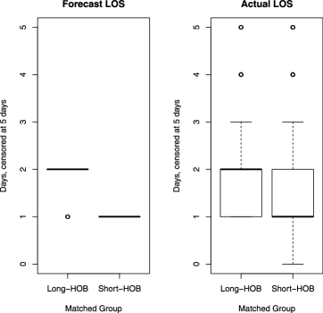
Figure 1: Anticipated and actual length of stay (LOS) in days in 80,600 matched pairs of a long-HOB baby and a short-HOB baby. The anticipated LOS for baby $ij$ is the median LOS for all babies with the same hour of birth (HOB) as baby $ij$. The figure on the left shows that babies in the long-HOB group were typically anticipated to stay two days (36–60 hours) while babies in the short-HOB group were anticipated to say one day (12–36 hours). The figure on the right is actual length of stay.

than 12 hours, one day as between 12 and 36 hours, two days as between 36 and 50 hours, and so on, in effect rounding to the nearest 24 hour unit. In Figure 1, the boxplots on the left for anticipated lengths of stay have collapsed into lines because the medians and quartiles are equal: typically, long-HOB babies were anticipated to stay two days and short-HOB babies were anticipated to stay one day. On the right in Figure 1, anticipation often but not always equaled actuality: the median and one quartile equaled the anticipated stay. Presumably, the decision to keep a baby in the hospital for four or more days in Figure 1 is not driven by the idiosyncrasy of hour of birth, but rather by serious health problems of the newborn. Table 5 describes the actual length of stay in pairs. Because babies were paired for important prognostic variables such as birth weight, it is not surprising that the two babies in pair often stayed the same number of days despite different hours-of-birth. Nonetheless, in a pair, when one baby stayed two days and the other stayed one, the odds were $18\mbox{,}746/8704=2.2$ to 1 that the long-HOB baby was the one who stayed two days.

Section 3 describes the new techniques used to construct this match and Section 4 presents an illustrative analysis of one important outcome, namely, readmission to the hospital within two days of discharge.

3 Using integer programming to construct the matched comparison.

3.1 Some algorithmic background: Integer versus network optimization.

An integer programming problem is essentially a linear programming problem in which the solution is restricted to have integer coordinates rather than fractional or real coordinates. Often, the solution is further restricted to a subset of the integers, sometimes to 0 or 1. An excellent introduction to integer programming is provided by Wolsey (1998) and a more detailed account is provided by Schrijver (1986). Integer programs arise in various problems in operations research because building $5.5$ submarines and $6.5$ destroyers is actually less sensible than building 6 submarines and 6 destroyers or 5 submarines and 7 destroyers or perhaps 8 submarines and 5 destroyers. Integer programming shows up in optimal matching because whole babies are matched to whole babies. Rounding the solution to a linear program may be substantially inferior to solving an integer program, but linear programming concepts play an important role in solving integer programs.

An integer program has the form

$$\mathop{\mathrm{minimize}}_{\mathbf{a}}\bolds{\eta}^{T}\mathbf{a}\quad\mbox{subject to}\quad\mathbf{Ba\leq b},\mathbf{a}\geq\mathbf{0}\qquad\mbox{with }\mathbf{a}\mbox{ integer},$$ (1)

where $\mathbf{B}$ is a given $d_{1}\times d_{2}$ matrix, $\bolds{\eta}$ is a given $d_{2}$-dimensional vector with real coordinates, $\mathbf{b}$ is a given $d_{1}$-dimensional vector, and one must find the best $d_{2}$-dimensional vector $\mathbf{a}$ with $d_{2}$ integer coordinates. The form (1) simplifies the discussion in the current section but, in general, integer programs may include both linear inequality constraints (as in $\mathbf{Ba\leq b}$) and linear equality constraints (say, $\mathbf{Ca=c}$) and, indeed, with a bit of juggling, either type of constraint may be reexpressed in terms of the other, so a separate theory for equality constraints is not needed. In the current paper and in most matching problems $\mathbf{a}$ is further restricted to have binary, 1 or 0, coordinates. The binary program is finite—there are $2^{d_{2}}$ candidate $\mathbf{a}$’s—but for large $d_{2}$ the number of candidates suffers a combinatorial explosion and considering all of them, one by one, is not possible. In the work here, $\bolds{\eta}$ and $\mathbf{a}$ have double subscripts, $\eta_{\ell m}$ and $a_{\ell m}$, $\ell<m$, where $\eta_{\ell m}$ is a measure of distance on covariates between babies $\ell$ and $m$, and $a_{\ell m}=1$ if babies $\ell$ and $m$ are paired and $a_{\ell m}=0$ if they are not. For instance, with $L$ babies, $\mathbf{a}=(a_{12},a_{13},a_{23},\ldots,a_{L-1,L})^{T}$. Then $\bolds{\eta}^{T}\mathbf{a}$ is the total covariate distance within matched pairs. The matrix $\mathbf{B}$ imposes various desired restrictions on the match, not least that each baby shows up in at most one pair.

In (1), if you remove the restriction that $\mathbf{a}$ is integral, then you have a linear program. The linear program always has a minimizing value of $\bolds{\eta}^{T}\mathbf{a}$ that is at least as small as the integer program, but again that leaves you with the rather damp prospect of half a submarine. There is a curious but important subset of problems in which the linear programming solution and the integer programming solution must be the same, and for these problems, known somewhat inaccurately as network optimization problems, especially fast algorithms are often available by adapting linear programming techniques. These problems are called “network optimization” because the most common versions arise from problems expressed in terms of the nodes and arcs of graph theory. Somewhat more precisely, there is an integral optimal solution to a linear programming problem if an integer matrix $\mathbf{B}$ is totally unimodular, that is, if every square submatrix of $\mathbf{B}$ has determinant $-1$, $0$, or $1$, a condition that insures via Cramer’s rule for matrix inversion that linear equations solve with integer solutions. See Wolsey [(1998), Section 3.2] for a precise statement and proof. In $\mathtt{R}$, Hansen’s (2007) optmatch package, Lu et al.’s (2011) nbpmatching package and Yang et al.’s (2012) finebalance package all use network optimization techniques, specifically the techniques of Bertsekas (1981) and Derigs (1988). The restriction of $\mathbf{B}$ to be totally unimodular is a substantial restriction, and one can do quite a bit more with (1) if $\mathbf{B}$ is not so restricted, a fact we demonstrate in detail in the current paper.

In abstract theory, solving large integer programs can be very difficult. In particular, the general problem (1) is NP-complete [Schrijver (1986), Section 18.1]; however, specific forms of (1) are polynomially bounded [e.g., Schrijver (1986), Section 18.6]. In practice, there has been a great deal of progress in solving quite large integer programs either exactly or approximately. We use IBMs ILOG program CPLEX to solve (1), and it is much faster than other programs we have tried. IBM makes CPLEX available to academics for free. Corrada Bravo (2005) created a package Rcplex that facilitates access to CPLEX inside R and we have used Rcplex on Apple and linux machines. In statistical matching, a common tactic is to match exactly for a few key covariates [Rosenbaum (2010), Section 9.3]—we did this for year and hospital—thereby breaking one large matching problem into several smaller ones, each of which can be solved quickly.

3.2 Nonbipartite matching using integer programming.

Generally, we wanted to match babies who were similar in terms of covariates but very different in terms of anticipated length of stay based on hour of birth. We matched exactly for hospital and year of birth, meaning that the two babies in a pair were born in the same year at the same hospital. Hospitals vary in discharge and readmission practices, so it was important to compare two babies in the same hospital. There have been substantial changes in discharge and readmission practices over the years, as well as advances in medical technique, so matching for year was also important. Exact matching can be implemented by simply dividing the population into mutually exclusive and exhaustive subpopulations, and performing a separate match for each subpopulation. Each subpopulaton consisted of a single hospital over an interval of years. The rest of the discussion describes the match within one such subpopulation, here a subpopulation defined by hospital and year of birth.

There are $L$ babies in the subpopulation, $\ell=1,\ldots,L$, and a variable $a_{\ell m}$, $1\leq\ell<m\leq L$, with $a_{\ell m}=1$ if babies $\ell$ and $m$ are paired and $a_{\ell m}=0$ otherwise. So $\mathbf{a}=(a_{12},\ldots,a_{L-1,L})^{T}$ has dimension ${L\choose 2}$ and $\mathbf{B}$ has ${L\choose 2}$ columns. The first constraint is that $a_{\ell m}\in\{0,1\}$ for all $\ell$, $m$, so the problem is not just an integer program but a binary program. Now each baby $\ell$ appears in at most one matched pair, and to enforce this, we impose $L$ linear inequalities, $\sum_{m=1}^{\ell-1}a_{m\ell}+\sum_{m=\ell+1}^{L}a_{\ell m}\leq 1$, for $\ell=1,\ldots,L$, which are coded as the first $L$ rows of $\mathbf{B}$, where $b_{1}=1,\ldots,b_{L}=1$.

In statistics, matching is almost invariably “without replacement,” meaning that no baby appears in more than one pair. The constraint $\sum_{m=1}^{\ell-1}a_{m\ell}+\sum_{m=\ell+1}^{L}a_{\ell m}\leq 1$ ensures matching is “without replacement.” Because outcome data are never used in constructing a match, when matching is without replacement, if the $L$ babies were independent prior to matching, then the pair outcomes are conditionally independent in distinct pairs given the variables used to construct the match, for instance, covariates and hour of birth. In contrast, in matching “with replacement,” babies would be used repeatedly in different pairs, creating dependence. The analysis in Section 4 uses existing techniques that are appropriate for conditionally independent pairs, but these existing techniques are inapplicable when matching “with replacement.” Indeed, even in the absence of bias from unmeasured covariates, Abadie and Imbens (2008) argue that straightforward applications of the bootstrap are inapplicable when matching “with replacement,” and that the specialized techniques of Abadie and Imbens (2006) or Politis and Romano (1994) are required to obtain a standard error.

Suppose $L$ is even and one further equality constraint is added, namely, $L/2=\sum_{m=1}^{L-1}\sum_{\ell=m+1}^{L}a_{m\ell}$ [so $\mathbf{B}$ has an $L+1$ row consisting of a vector with ${L\choose 2}$ coordinates all equal to 1]. Then setting $\eta_{\ell m}$ equal to a covariate distance between babies $\ell$ and $m$ and solving (1) would yield a minimum distance nonbipartite match that divides the $L$ babies into $L/2$ nonoverlapping pairs to minimize the total of the $L/2$ distances within pairs. This optimization problem can be solved quickly using network techniques [Derigs (1988)] as implemented in R in the nbpmatching package [Lu et al. (2011)].

In contrast, the remainder of this section imposes additional constraints as additional rows of $\mathbf{B}$ to achieve specific effects, and these require the integer programming formulation. In Section 3.2.1, the marginal distributions of several nominal variables are forced to balance exactly, a condition known as fine balance, as seen in Tables 1 and 2. In Section 3.2.2, a binary requirement is imposed on pairs, while permitting a small fraction of pairs to escape the requirement as needed, a condition which together with fine balance produced Table 4 for low birth weight, with perfect balance for marginal distributions combined with most pairs exactly matched. Section 3.2.3 forces the means of a continuous covariate to balance, as seen for birth weight in Table 3, while Section 3.2.5 forces the means of the instrument to differ, thereby strengthening the instrument, as seen in Figure 1. Fine balance is generalized to near-fine balance in Section 3.2.4. Finally, Section 3.2.7 adjusts $\eta_{\ell m}$ to optimize deletion of some babies while making the remaining babies closer on covariates and further apart on the instrument.

In teaching, multiple linear regression is defined abstractly, and then specific ways of coding its predictor matrix are shown to fit useful models, such as polynomials or interactions. In parallel, the integer programming solution to nonbipartite matching is best viewed abstractly as (1) with $a_{\ell m}\in\{0,1\}$ and the first $L$ rows of $\mathbf{B}$ requiring $\sum_{m=1}^{\ell-1}a_{m\ell}+\sum_{m=\ell+1}^{L}a_{\ell m}\leq 1$. Then one obtains a match that meets specific requirements by suitably adjusting $\mathbf{B}$ and $\eta_{\ell m}$, as described in Sections 3.2.1–3.2.7.

3.2.1 Fine balance.

Table 2 exhibits fine balance of the marginal distributions for the seven nominal variables. Fine balance for a covariate means that the marginal distributions of the covariate are exactly the same in matched treated and control groups, although individual pairs may not be exactly matched for this covariate. If a nominal variable has $C$ categories, it is represented as $C-1$ binary indicators. Let $w_{\ell}$ be the binary indicator for one such category, say, $w_{\ell}=1$ if baby $\ell$ is Hispanic and $w_{\ell}=0$ if baby $\ell$ is not Hispanic. Fine balance for this category is the linear equality constraint

$$\sum_{\ell=1}^{L-1}\sum_{m=\ell+1}^{L}a_{\ell m}(w_{\ell}-w_{m})=0.$$ (2)

Fine balance in Table 2 is actually present in every year in every hospital; that is, for instance, among babies born in 2000 in hospital 22, the number of Hispanic long-HOB babies equals the number of Hispanic short-HOB babies. Fine balance was imposed through several linear equality constraints of this form. In principle, an equality constraint (2) may be expressed in the formulation (1) as two inequalities or two rows of $\mathbf{B}$, namely, $\sum_{\ell=1}^{L-1}\sum_{m=\ell+1}^{L}a_{\ell m}(w_{\ell}-w_{m})\leq 0$ and $\sum_{\ell=1}^{L-1}\sum_{m=\ell+1}^{L}a_{\ell m}(w_{m}-w_{\ell})\leq 0$; however, most solvers including CPLEX accept either inequality or equality constraints. In CPLEX, each fine balance constraint (2) becomes one additional row of $\mathbf{B}$ with an equality constraint.

Treated-versus-control minimum distance matching with fine balance for one nominal variable, possibly with many levels, was proposed in Rosenbaum [(1989), Section 3.2] and Rosenbaum, Ross and Silber (2007) using either network optimization or the optimal assignment algorithm; however, that approach is not applicable in nonbipartite matching and can only balance one nominal variable. In contrast, the integer programming formulation of fine balance (2) is applicable to nonbipartite matching while balancing one or more variables.

3.2.2 Binary requirements for individual pairs.

Let $h_{\ell m}\in\{0,1\}$ be a binary variable describing the pairing of two babies, $\ell$ and $m$, where we wish to sharply limit the number of times that paired babies have $h_{\ell m}=1$, say, to at most $H$ pairs. Taking $H=0$ requires $h_{\ell m}=0$ for all $\ell$ and $m$, whereas taking $H=5$ permits at most five matched pairs to have $h_{\ell m}=1$. In this study, we wanted paired babies to differ substantially in terms of anticipated length of stay, so we set $h_{\ell m}=1$ whenever baby $\ell$ had an anticipated length of stay that was less than 12 hours more than the anticipated length of stay for baby $m$. The linear inequality constraint

$$\sum_{\ell=1}^{L-1}\sum_{m=\ell+1}^{L}a_{\ell m}h_{\ell m}\leq H$$ (3)

is added as a row to $\mathbf{B}$ to impose this constraint with $H=0$. In addition, within each hospital in each year, a constraint of the form (3) was used with $h_{\ell m}=1$ if babies $\ell$ and $m$ differed in terms of low birth weight $<2500$ grams and $H$ was twenty percent of the number of births in that hospital in that year.

3.2.3 Balancing means.

For any covariate $v$, not necessarily a binary covariate, suppose that we wish to ensure that the means in matched treated and controls groups differ by at most a number $\varepsilon>0$. Unlike a binary covariate in (2), for a continuous covariate such as birth weight, one cannot reasonably take $\varepsilon=0$. Because there are $\sum_{\ell=1}^{L-1}\sum_{m=\ell+1}^{L}a_{\ell m}$ matched pairs, this requirement is the same as

$$\Biggl{|}\sum_{\ell=1}^{L-1}\sum_{m=\ell+1}^{L}a_{\ell m}v_{\ell}-\sum_{\ell=1}^{L-1}\sum_{m=\ell+1}^{L}a_{\ell m}v_{m}\Biggr{|}\leq\varepsilon\sum_{\ell=1}^{L-1}\sum_{m=\ell+1}^{L}a_{\ell m}.$$ (4)

Now, because of the absolute values in the constraint (4), this constraint is not one linear inequality. However, requiring (4) to hold is equivalent to requiring two linear inequalities to both hold, namely,

$$\sum_{\ell=1}^{L-1}\sum_{m=\ell+1}^{L}a_{\ell m}(v_{\ell}-v_{m}-\varepsilon)\leq 0\quad\mbox{and}\quad\sum_{\ell=1}^{L-1}\sum_{m=\ell+1}^{L}a_{\ell m}(v_{m}-v_{\ell}-\varepsilon)\leq 0.$$ (5)

So, a requirement that the means of $v$ after matching differ by at most $\varepsilon$ is represented in the integer program as two rows of the matrix $\mathbf{B}$. Notice in Table 3 that the mean of birth weight is almost the same for the long-HOB and short-HOB babies. The same technique was applied to birth injury and oligohydramnios in Table 3.

3.2.4 Near-fine balance.

Sometimes fine balance (2) for a binary variable $w$ is infeasible or just too restrictive. For bipartite matching, Yang et al. (2012) proposed a network optimization algorithm for treatment-versus-control near-fine balance requiring $|\sum_{\ell=1}^{L-1}\sum_{m=\ell+1}^{L}a_{\ell m}(w_{\ell}-w_{m})|\leq\varepsilon$ rather than (2) for the binary variables $w$ that define categories of a single nominal variable, and Yang implemented this in her finebalance package in R which uses network optimization. Just as (4) became two linear inequalities in (5), so too $|\sum_{\ell=1}^{L-1}\sum_{m=\ell+1}^{L}a_{\ell m}(w_{\ell}-w_{m})|\leq\varepsilon$ may be split into two linear inequality constraints which are imposed using integer programming. Also, unlike network optimization, integer programming permits near-fine balance for one or more nominal variables in nonbipartite matching.

3.2.5 Forcing pairs to differ with respect to the mean of the instrument.

Although we set a minimum requirement of a 12 hour difference in anticipated length of stay using a constraint of the form (3), we wanted the typical difference to be larger than the minimum. Specifically, we imposed the requirement that the mean difference in anticipated length of stay, say, $v_{\ell}$, should be at least $\phi=13$ hours, that is, we required

$$\sum_{\ell=1}^{L-1}\sum_{m=\ell+1}^{L}a_{\ell m}v_{\ell}-\sum_{\ell=1}^{L-1}\sum_{m=\ell+1}^{L}a_{\ell m}v_{m}\geq\phi\sum_{\ell=1}^{L-1}\sum_{m=\ell+1}^{L}a_{\ell m}$$

by imposing the linear inequality constraint

$$\sum_{\ell=1}^{L-1}\sum_{m=\ell+1}^{L}a_{\ell m}(v_{\ell}-v_{m}-\phi)\geq 0.$$

In Table 3, the anticipated length of stay based on birth hour is 39.56 hours for the long-HOB babies and 25.48 hours for the short-HOB babies, an anticipated difference of more than 14 hours.

3.2.6 Using several techniques to balance one covariate.

It is possible to use several of these devices for the same variable. Birth weight is an especially important prognostic variable. We finely balanced the indicator of birth weight $<2500$ grams in Table 2 using a constraint of the form (2). We limited the difference in means of birth weight in Table 3 using a pair of constraints of the form (5), and we limited the number of times individual pairs $(\ell,m)$ were mismatched for the indicator of birth weight $<2500$ grams using a constraint of the form (3).

3.2.7 Optimal selection of a subset.

Recall that our match discards some babies and must optimally decide the following: (i) how many babies to discard, (ii) which babies to discard, and (iii) how to pair the babies not discarded. Extending the technique in Rosenbaum (2012) to nonbipartite matching, the objective function $\bolds{\eta}^{T}\mathbf{a}$ is

$$\sum_{\ell=1}^{L-1}\sum_{m=\ell+1}^{L}a_{\ell m}\omega_{\ell m}-\lambda\sum_{\ell=1}^{L-1}\sum_{m=\ell+1}^{L}a_{\ell m}$$ (6)

or $\eta_{\ell m}=\omega_{\ell m}-\lambda$, where $\omega_{\ell m}$ is a robust Mahalanobis distance between the covariates for babies $\ell$ and $m$, and $\lambda$ is a constant selected by the investigator. For discussion of the use of Mahalanobis distances in matching, see Rubin (1980), and for a robust Mahalanobis distance, see Rosenbaum (2010), Sections 8.3 and 13.11. Because $\sum_{\ell=1}^{L-1}\sum_{m=\ell+1}^{L}a_{\ell m}$ is the number of matched pairs, the objective function (6) has the following interpretation. When comparing two possible matched samples, say, $a_{\ell m}$ and $a_{\ell m}^{{\prime}}$, that satisfy the constraints with the same number of pairs, (6) prefers the pairing with the smaller total distance within pairs. Suppose, instead, $a_{\ell m}$ includes $A>0$ more pairs than $a_{\ell m}^{{\prime}}$, $A=\sum_{\ell=1}^{L-1}\sum_{m=\ell+1}^{L}a_{\ell m}-a_{\ell m}^{{\prime}}$. Then (6) prefers $a_{\ell m}^{{\prime}}$ to $a_{\ell m}$ if

$$\sum_{\ell=1}^{L-1}\sum_{m=\ell+1}^{L}a_{\ell m}^{{\prime}}\omega_{\ell m}-\lambda\sum_{\ell=1}^{L-1}\sum_{m=\ell+1}^{L}a_{\ell m}^{{\prime}}<\sum_{\ell=1}^{L-1}\sum_{m=\ell+1}^{L}a_{\ell m}\omega_{\ell m}-\lambda\sum_{\ell=1}^{L-1}\sum_{m=\ell+1}^{L}a_{\ell m}$$

or, equivalently, if

$$\frac{\sum_{\ell=1}^{L-1}\sum_{m=\ell+1}^{L}a_{\ell m}\omega_{\ell m}-\sum_{\ell=1}^{L-1}\sum_{m=\ell+1}^{L}a_{\ell m}^{{\prime}}\omega_{\ell m}}{\sum_{\ell=1}^{L-1}\sum_{m=\ell+1}^{L}a_{\ell m}-\sum_{\ell=1}^{L-1}\sum_{m=\ell+1}^{L}a_{\ell m}^{{\prime}}}>\lambda.$$ (7)

In words, the match represented by $a_{\ell m}$ had $A$ pairs more than the match $a_{\ell m}^{{\prime}}$, so the sum of the distances $\omega_{\ell m}$ for $a_{\ell m}$ contained $A$ more distances, and the total distance within pairs rose by more than $A\lambda$ if (7) holds, so the average cost of these $A$ additional pairs was more than $\lambda$. The objective (6) prefers more pairs to fewer pairs if, on average, more pairs may be had for less than $\lambda$ and prefers fewer pairs if, on average, they cost more than $\lambda$. Because $a_{\ell m}$ and $a_{\ell m}^{{\prime}}$ pair babies differently, the change in average cost is produced by all of the paired babies, not just $A$ babies; see Rosenbaum (2012) for detailed discussion. In our case, $\lambda$ was the median of all distances before matching, and the algorithm prefers more pairs to fewer pairs providing the added pairs are, on average, closer than pairs typically are. Of 231,831 babies, this value of $\lambda$ paired 161,200 babies. Although it would be possible to pair additional babies, each of these additions would, on average, raise the distance by more than $\lambda$, that is, by more than the median pairwise distance before matching. One might choose a different $\lambda$ in a different context.

3.3 Comparison with three other matched samples.

Table 6 compares the match described in Section 2 with three other sets of matched pairs. As noted in Section 3.2, the match in Section 2 insisted on a separation of 12 hours in anticipated length-of-stay within each pair. Table 6 contrasts matching with 12 hour separation to matching with no required separation, $\geq$9 hours and $\geq$15 hours. Two quantities are reported in Table 6: the number of pairs and the percent of babies staying more than one day, where one day is a length-of-stay between 12 and 36 hours. With $0$ separation, there is only a 6.2% difference between long-HOB and short-HOB births in stays more than one day. With 12 hours of separation, the difference is more than twice as large, 13.4%. In the terminology of Angrist, Imbens and Rubin (1996), the percent of compliers is estimated to be more than twice as large with 12 hours of separation as with 0 separation.

=260pt Separation in anticipated LOS Hours $0$ $9$ $12$ $15$ Long-HOB % $46.9$ $50.2$ $52.7$ $58.7$ Short-HOB % $40.7$ $38.0$ $39.2$ $41.8$ Difference % $6.2$ $12.1$ $13.4$ $16.9$ Number of pairs 91,053 90,360 80,600 59,678

Table 6: Comparison of four the actual match required samples with different required differences in anticipated length of stay. The actual matched required a 12 hour difference in anticipated length of stay. This 12 hour required difference is compared with 0, 9 and 15 hours. The table records the percent of babies staying longer than one day and the number of pairs. Because zero days is a length of stay less than 12 hours, and one day is a length of stay greater than 12 hours but less than 36 hours, the table indicates the percent of babies staying longer than 36 hours

Matching is part of the design of an observational study, a task that should be completed before outcomes are examined [Langenskiold and Rubin (2008), Rosenbaum (2010)], and, in particular, one matched sample should be selected as the design without using or examining outcomes. We selected the 12 hour match based on its qualities as a matched comparison, for instance, the covariate balance in Tables 1–5 and Figure 1, and the number of pairs and instrument strength in Table 6. The analysis of outcomes for this selected match is discussed in Section 4.

4 Inference: Effects on rapid readmission.

4.1 Null hypotheses of no effect or substantial inequivalence.

We will conduct both a test of no effect and an equivalence test for readmissions within two days of discharge from the hospital. That is, we wish to ask whether our data are compatible with no effect or substantial effects of shifting the norm for length of stay. Following Bauer and Kieser (1996), a three part null hypothesis is tested, where one part asserts no effect, a second part asserts moderately large benefits from a 2-day norm and the third part asserts moderately large benefits from a 1-day norm. Because these three null hypotheses are logically incompatible with one another, at most one of the null hypotheses is true, so all three hypotheses may be tested without a correction for testing multiple hypotheses; see Bauer and Kieser (1996). In particular, the hypothesis of no effect is a two-sided hypothesis saying changing the hour of birth for a baby would not change whether the baby is readmitted within two days of discharge. The hypothesis that a norm of a one-day length-of-stay is harmful asserts that it caused at least 500 readmissions that would not have occurred with a two-day norm. Because there are $80\mbox{,}600$ pairs in Table 7, each pair containing one short-HOB baby, 500 readmissions is slightly more

=220pt Observed data Short-HOB baby Long-HOB baby Not readmitted Readmitted Not readmitted 78,431 1032 Readmitted ,01108 0029

Table 7: Readmission within two days of discharge in matched pair. The table counts pairs, not babies

than one half of one percent of these babies (actually $500/80\mbox{,}600=0.00620$). In Table 5, $18\mbox{,}746-8704=10\mbox{,}042$ more long-HOB babies stayed 2 days rather than 1 day, and 500 babies is about 5% of these 10,042 babies (actually $500/10\mbox{,}042=0.0498$). The same value, 500, is used to test the third hypothesis of substantial harm, rather than substantial benefit, from a two-day norm. In testing these hypotheses, we are concerned about both sampling variability and bias from nonrandom treatment assignment.

4.2 Randomization inference in matched pairs: Viewing hour of birth as random.

There are $I$ matched pairs, $i=1,\ldots,I$ of two babies, $j=1,2$, one treated, $Z_{ij}=1$, the other control, $Z_{ij}=0$, so $Z_{i1}+Z_{i2}=1$ for each $i$. In Section 1.2, there were $I=80\mbox{,}600$ pairs of babies, or $2\times 80\mbox{,}600=161\mbox{,}200$ babies in total, and somewhat arbitrarily we designate short-HOB as treatment and long-HOB as control. Babies were matched for an observed covariate $\mathbf{x}_{ij}$, so $\mathbf{x}_{i1}=\mathbf{x}_{i2}$ for all $i$, but they may have differed in terms of an unmeasured covariate $u_{ij}$, so quite possibly $u_{i1}\neq u_{i2}$ for many or all $i$. Write $\mathbf{Z}=(Z_{11},\ldots,Z_{I2})^{T}$ for the $2I$-dimensional vector of treatment assignments and write $\mathcal{Z}$ for the set containing the $2^{I}$ possible values $\mathbf{z}$ of $\mathbf{Z}$, so $\mathbf{z}\in\mathcal{Z}$ if $\mathbf{z}=(z_{11},\ldots,z_{I2})^{T}$ with $z_{ij}=0$ or $z_{ij}=1$ and $z_{i1}+z_{i2}=1$ for each $i$. If $\mathcal{S}$ is a finite set, write $|\mathcal{S}|$ for the number of elements of $\mathcal{S}$, so $|\mathcal{Z}|=2^{I}$. Conditioning on the event $\mathbf{Z}\in\mathcal{Z}$ is abbreviated to conditioning on $\mathcal{Z}$.

Each baby has two potential binary 1 or 0 responses, $r_{Tij}$ if treated, $r_{Cij}$ if control, so the effect of the treatment on this baby, namely, $\delta_{ij}=r_{Tij}-r_{Cij}$, is not seen for any baby $ij$ but the response actually seen from $ij$ is $R_{ij}=Z_{ij}r_{Tij}+(1-Z_{ij})r_{Cij}=r_{Cij}+Z_{ij}\delta_{ij}$; see Neyman (1923), Welch (1937), Rubin (1974), Reiter (2000) or Gadbury (2001). Write $\mathbf{R}=(R_{11},\ldots,R_{I2})^{T}$, $\bolds{\delta}=(\delta_{11},\ldots,\delta_{I2})^{T}$, $\mathbf{r}_{C}=(r_{C11},\ldots,r_{CI2})^{T}$, $\mathbf{r}_{T}=(r_{T11},\ldots,r_{TI2})^{T}$, so $\mathbf{r}_{T}=\mathbf{r}_{C}+\bolds{\delta}$. Here, $\delta_{ij}\in\{-1,0,1\}$ for each $ij$ and Fisher’s (1935) sharp null hypothesis $H_{0}$ of no treatment asserts that $H_{\mathbf{0}}:\bolds{\delta}=\mathbf{0}$. In the discussion here, $R_{ij}$ indicates whether baby $ij$ was readmitted, $R_{ij}=1$, or not, $R_{ij}=0$, within two days of discharge from the hospital. If $r_{Tij}=1$ and $r_{Cij}=0$ so $\delta_{ij}=r_{Tij}-r_{Cij}=1$, then baby $ij$ would have been readmitted if born at an hour that would typically lead to a one-day stay and would not have been readmitted if born at an hour that would typically lead to a two-day stay, so being born at a short-HOB rather than a long-HOB would have caused this baby to be readmitted. Aside from Fisher’s null hypothesis of no effect, greatest interest attaches to hypotheses in which one treatment may cause but does not prevent a readmission, $H_{\bolds{\delta}_{0}}:\bolds{\delta}=\bolds{\delta}_{0}$ with $\bolds{\delta}_{0}\geq\mathbf{0}$ and $\bolds{\delta}_{0}\neq\mathbf{0}$, because hypotheses of this form say that one treatment is clearly better than the other. Write $\mathcal{F}=\{(r_{Tij},r_{Cij},\mathbf{x}_{ij},u_{ij}),i=1,\ldots,I,j=1,2\}$ for the potential responses and covariates.

In a paired randomized experiment, one baby in each pair would be picked at random for treatment, the other baby receiving control, with independent assignments in distinct pairs, that is, $\Pr(\mathbf{Z}=\mathbf{z}|\mathcal{F},\mathcal{Z})=2^{-I}$ for $\mathbf{z}\in\mathcal{Z}$. In Section 1.2, hour-of-birth is not randomized, but because hour of birth should not pick out a particular type of baby, the hope is that $\Pr(\mathbf{Z}=\mathbf{z}|\mathcal{F},\mathcal{Z})$ is close to the randomization distribution. Section 4.3 examines the sensitivity of conclusions to departures of various magnitudes from $\Pr(\mathbf{Z}=\mathbf{z}|\mathcal{F},\mathcal{Z})=2^{-I}$.

The statistic $T=\sum_{i=1}^{I}\sum_{j=1}^{2}Z_{ij}R_{ij}$ is the observed number of readmissions within two days among babies born at a short-HOB. Some of the readmissions recorded in $T$ may have been caused by the short-HOB and others might have occurred whether the baby was born at a short or a long HOB. The unobservable quantity $T_{c}=\sum_{i=1}^{I}\sum_{j=1}^{2}Z_{ij}r_{Cij}$ is the number of readmissions that would have occurred had all babies been born at a long-HOB. Fisher’s sharp null hypothesis, $H_{\mathbf{0}}:\bolds{\delta}=\mathbf{0}$, says that no readmission was caused or prevented by the hour of birth, with the consequence that $T=T_{c}$. Consider the distribution of $T_{c}$ in a randomized experiment, that is, $\Pr(T_{c}\leq k|\mathcal{F},\mathcal{Z})$ when $\Pr(\mathbf{Z}=\mathbf{z}|\mathcal{F},\mathcal{Z})=2^{-I}$. Define $n_{11}$ to be the number of pairs $i$ with $r_{Ci1}=r_{Ci2}=1$, $n_{00}$ to be the number of pairs with $r_{Ci1}=r_{Ci2}=0$, and $n_{10}$ to be the number of pairs with $r_{Ci1}\neq r_{Ci2}$. If $H_{\mathbf{0}}:\bolds{\delta}=\mathbf{0}$ were true, then $R_{ij}=r_{Cij}$ and it would be possible to calculate $(n_{11},n_{10},n_{00})$ from the observed $R_{ij}$’s. Because $\Pr(\mathbf{Z}=\mathbf{z}|\mathcal{F},\mathcal{Z})=2^{-I}$ and $\mathbf{r}_{C}$ is fixed by conditioning on $\mathcal{F}$, the $I$ terms $\sum_{j=1}^{2}Z_{ij}r_{Cij}$ are independent for distinct $i$, and $\sum_{j=1}^{2}Z_{ij}r_{Cij}$ is 1 with certainty if the pair is concordant with $r_{Ci1}=r_{Ci2}=1$, is 0 with certainty if the pair is concordant with $r_{Ci1}=r_{Ci2}=0$, and is 1 or 0 each with probability $\frac{1}{2}$ if the pair is discordant with $r_{Ci1}\neq r_{Ci2}$; therefore, $T_{c}$ is the constant $n_{11}$ plus a binomial random variable with probably of success $\frac{1}{2}$ and sample size $n_{10}$. Because $T=T_{c}$ when Fisher’s sharp null hypothesis $H_{\mathbf{0}}:\bolds{\delta}=\mathbf{0}$ is true, it follows that $H_{0}$ may be tested in a randomized experiment by comparing $T$ with the randomization distribution of $T_{c}$, and this is essentially the same as McNemar’s test.

Let $\bolds{\delta}_{0}$ be a $2I$-dimensional with coordinates $\delta_{0ij}\in\{-1,0,1\}$, and consider the hypothesis $H_{\bolds{\delta}_{0}}:\bolds{\delta}=\bolds{\delta}_{0}$. Not all hypotheses of this form are logically compatible with the observed data because $R_{ij}-Z_{ij}\delta_{ij}=r_{Cij}$ and $R_{ij}+(1-Z_{ij})\delta_{ij}=r_{Tij}$ must both be in $\{0,1\}$. If $H_{\bolds{\delta}_{0}}$ is logically incompatible with the data, we may reject it with type 1 error rate of zero, so for the remainder of the discussion, assume that $H_{\bolds{\delta}_{0}}$ is logically compatible with the observed data, or briefly compatible. If $H_{\bolds{\delta}_{0}}:\bolds{\delta}=\bolds{\delta}_{0}$ were true (and hence compatible), then $r_{Cij}=R_{ij}-Z_{ij}\delta_{0ij}$ may be calculated from the hypothesis and the data, so $n_{11}$, $n_{10}$, $n_{00}$ and $T_{c}$ may be calculated as well, so $T_{c}$ may be compared with the constant-plus-binomial distribution to test $H_{\bolds{\delta}_{0}}$. Unfortunately, there are many hypotheses $H_{\bolds{\delta}_{0}}:\bolds{\delta}=\bolds{\delta}_{0}$ and it is not practical to test them all; however, the testing of many hypotheses $H_{\bolds{\delta}_{0}}:\bolds{\delta}=\bolds{\delta}_{0}$ may be summarized using a scalar quantity, the attributable effect.

The attributable effect $\Delta=\sum_{i=1}^{I}\sum_{j=1}^{2}Z_{ij}\delta_{ij}$ is an unobservable quantity giving the net increase in the number of babies readmitted because they were born at a short-HOB; see Rosenbaum (2002a). It is a random variable because it depends upon $\mathbf{Z}$, but it is not an observable random variable because it depends on $\bolds{\delta}$. Among babies born at a short-HOB, we see $T=\sum_{i=1}^{I}\sum_{j=1}^{2}Z_{ij}R_{ij}=\sum_{i=1}^{I}\sum_{j=1}^{2}Z_{ij}r_{Tij}$ readmissions, whereas these same babies would have had $T_{c}=\sum_{i=1}^{I}\sum_{j=1}^{2}Z_{ij}r_{Cij}$ readmissions had they been born at a long-HOB. If $H_{\bolds{\delta}_{0}}:\bolds{\delta}=\bolds{\delta}_{0}$ were true, then $\Delta$ may be calculated using the hypothesized $\bolds{\delta}_{0}$ as $\Delta_{0}=\sum_{i=1}^{I}\sum_{j=1}^{2}Z_{ij}\delta_{0ij}$, and $T-\Delta_{0}$ would equal $T_{c}$.

For the reason noted above, we consider hypotheses $H_{\bolds{\delta}_{0}}:\bolds{\delta}=\bolds{\delta}_{0}$ that say that one treatment is better than the other in the sense that $\bolds{\delta}_{0}\geq\mathbf{0}$ and $\bolds{\delta}_{0}\neq\mathbf{0}$. We will do this twice, once reversing the roles of treatment and control, but for the moment consider the hypothesis that a short-HOB may cause but not prevent readmissions in the sense that $\bolds{\delta}_{0}\geq\mathbf{0}$. A value of $\Delta_{0}$ is rejected if every hypothesis $H_{\bolds{\delta}_{0}}:\bolds{\delta}=\bolds{\delta}_{0}$ with $\bolds{\delta}_{0}\geq\mathbf{0}$ and $\bolds{\delta}_{0}\neq\mathbf{0}$ that gives rise to this value of $\Delta_{0}=\sum_{i=1}^{I}\sum_{j=1}^{2}Z_{ij}\delta_{0ij}$ is rejected; otherwise, this value of $\Delta_{0}$ is not rejected. For all of these hypotheses, $T-\Delta_{0}=T_{c}$ will be the same number; however, $n_{11}$, $n_{10}$ and $n_{00}$ typically change with $\bolds{\delta}_{0}$. For a given $\Delta_{0}$, among all hypotheses $H_{\bolds{\delta}_{0}}:\bolds{\delta}=\bolds{\delta}_{0}$ with $\bolds{\delta}_{0}\geq\mathbf{0}$ and $\bolds{\delta}_{0}\neq\mathbf{0}$ that yield the same attributable effect $\Delta_{0}$, there is one hypothesis $H_{\widetilde{\bolds{\delta}}_{0}}:\bolds{\delta}=\widetilde{\bolds{\delta}}_{0}$ with $\Delta_{0}=\sum_{i=1}^{I}\sum_{j=1}^{2}Z_{ij}\widetilde{\delta}_{0ij}$ that is the most difficult to reject, so if $H_{\widetilde{\bolds{\delta}}_{0}}$ is rejected, then the associated value of $\Delta_{0}$ is rejected. In a cohort study, as in Section 1.2, this hypothesis $H_{\widetilde{\bolds{\delta}}_{0}}:\bolds{\delta}=\widetilde{\bolds{\delta}}_{0}$ has $\sum_{j=1}^{2}Z_{ij}\delta_{ij}=1$ for as many pairs with $R_{i1}+R_{i2}=2$ as possible; see Rosenbaum [(2002a), Section 6] for a precise statement and proof. For instance, if Table 7 had come from a randomized experiment, $\Pr(\mathbf{Z}=\mathbf{z}|\mathcal{F},\mathcal{Z})=2^{-I}$, then $\Delta_{0}\geq 500$ would be rejected if McNemar’s one-sided test rejected no effect in the adjusted Table 8, where all 29 pairs with $R_{i1}+R_{i1}=2$ have $\widetilde{\delta}_{0ij}=1$ and 471 pairs with $R_{i1}+R_{i1}=1$ have $\widetilde{\delta}_{0ij}=1$. Why is this $H_{\widetilde{\bolds{\delta}}_{0}}$ the hypothesis that is most difficult to reject among hypotheses with $\Delta_{0}\geq 500$? Intuitively, this $H_{\widetilde{\bolds{\delta}}_{0}}$ has $\Delta_{0}=500$ with the most variability because the number of discordant pairs $n_{10}$ is as large as possible; see Rosenbaum [(2002a), Section 6] for precise discussion.

=240pt Data adjusted for $\bolds{H_{0}\dvtx\bolds{\delta}=\bolds{\delta}_{0}}$ Short-HOB baby Long-HOB baby Not readmitted Readmitted Not readmitted 78,902 561 Readmitted 01137 000

Table 8: Readmission within two days of discharge in matched pair adjusted for a null hypothesis $H_{0}\dvtx\bolds{\delta}=\bolds{\delta}_{0}$ that attributes $\sum\delta_{ij}Z_{ij}=\Delta=500$ readmissions to early discharge

If Table 7 had been seen in a randomized experiment, $\Pr(\mathbf{Z}=\mathbf{z}|\mathcal{F},\mathcal{Z})=2^{-I}$, then the procedure just described would yield the following conclusions. Testing the null hypothesis of no effect, $H_{\mathbf{0}}:\bolds{\delta}=\mathbf{0}$, yields a two-sided $P$-value of 0.105 using McNemar’s two-sided test, so no effect is plausible. Is a substantial benefit of $\Delta_{0}=500$ from being born at a long-HOB also plausible? It is not. McNemar’s one-sided test rejects in Table 8 with $P$-value $2.1\times 10^{-45}$, so it rejects for every $H_{\bolds{\delta}_{0}}:\bolds{\delta}=\bolds{\delta}_{0}$ with $\bolds{\delta}_{0}\geq\mathbf{0}$ and $\bolds{\delta}_{0}\neq\mathbf{0}$ and $\Delta_{0}\geq 500$. Reversing the roles of (and notation for) a short-HOB and a long-HOB, a substantial benefit of $\Delta_{0}=500$ from being born at a short-HOB is rejected with a $P$-value $2.9\times 10^{-25}$. In brief, if Table 7 had been seen in a randomized experiment, the hypothesis of no effect would be plausible, whereas a benefit or harm that affected at least one half of one percent of babies would not be remotely plausible. Of course, Table 7 is not from a randomized experiment.

Our hope has been that a baby’s hour of birth tells you little or nothing about the baby and her mother, that is, our hope was that hour of birth was nearly random, at least after matching for covariates. We cannot be certain of this, however. It is possible to use drugs to induce or accelerate labor, and perhaps the use of such drugs shifts the hour of delivery for some mothers, possibly in a fashion that biases randomization inferences based on Table 7. Moreover, the distribution of times for vaginal delivery may be affected by cesarean sections, which again may be related to aspects of the mother or the hospital. How large would such biases have to be to alter the qualitative conclusions based on randomization inferences? This is examined in Section 4.3 using a sensitivity analysis.

4.3 Sensitivity analysis in matched pairs: What if birth hour is not random?

The assumption in Section 4.2 was that hour of birth is effectively random, that it tells you nothing about the baby or the mother or the hospital and its staff, so that $\Pr(\mathbf{Z}=\mathbf{z}|\mathcal{F},\mathcal{Z})=2^{-I}$ for $\mathbf{z}\in\mathcal{Z}$. The current section studies sensitivity of the conclusions to quantified violations of this assumption. The model (9) for sensitivity analysis used here is discussed in Rosenbaum (2002b), Section 4. Other methods of sensitivity analysis in observational studies are discussed by Cornfield et al. (1959), Rosenbaum and Rubin (1983), Yanagawa (1984), Gastwirth (1992), Marcus (1997), Imbens (2003), Diprete and Gangl (2004), Yu and Gastwirth (2005), Wang and Krieger (2006), McCandless, Gustafson and Levy (2007), Egleston, Scharfstein and MacKenzie (2009) and Hosman, Hansen and Holland (2010), among others.

One model for sensitivity analysis in observational studies asserts that, in the population before matching, treatment assignments are independent and two babies, say, $ij$ and $ij^{\prime}$, with the same observed covariates, $\mathbf{x}_{ij}=\mathbf{x}_{ij^{\prime}}$, may differ in their odds of treatment by at most a factor of $\Gamma\geq 1$,

$$\frac{1}{\Gamma}\leq\frac{\Pr(Z_{ij}=1|\mathcal{F})\Pr(Z_{ij^{\prime}}=0|\mathcal{F})}{\Pr(Z_{ij}=0|\mathcal{F})\Pr(Z_{ij^{\prime}}=1|\mathcal{F})}\leq\Gamma;$$ (8)

then the distribution of $\mathbf{Z}$ is returned to $\mathcal{Z}$ by conditioning on $\mathbf{Z}\in\mathcal{Z}$. Model (8) is similar to the sensitivity analysis of Cornfield et al. (1959) and is exactly the same as assuming that

$$\Pr(\mathbf{Z}=\mathbf{z}|\mathcal{F},\mathcal{Z}) = \prod_{i=1}^{I}\frac{\exp(\sum_{j=1}^{2}\gamma z_{ij}u_{ij})}{\exp(\gamma u_{i1})+\exp(\gamma u_{i2})}$$ (9)

$$= \frac{\exp(\gamma\mathbf{u}^{T}\mathbf{z})}{\sum_{\mathbf{b}\in\mathcal{Z}}\exp(\gamma\mathbf{u}^{T}\mathbf{b})}\qquad\mbox{with }\mathbf{u}\in[0,1]^{2I}\mbox{ and }\gamma=\log(\Gamma);$$ (10)

see Rosenbaum [(2002b), Section 4] where $u_{ij}$ satisfying (9) is constructed from $\Pr(Z_{ij}=1|\mathcal{F})$ satisfying (8) and conversely.

Using either of the two approaches in Gastwirth, Krieger and Rosenbaum (1998) or Rosenbaum and Silber (2009b), the one parameter $\Gamma$ may be unpacked into two sensitivity parameters, one controlling the relationship between $u_{ij}$ and treatment $Z_{ij}$, the other controlling the relationship between $u_{ij}$ and response under control $r_{Cij}$. For instance, an unobserved covariate $u_{ij}$ that both doubles the odds of a short-HOB and doubles the odds of readmission within two days is equivalent to $\Gamma=1.25$, whereas doubling the odds of a short-HOB with a four-fold increase in the odds of readmission is equivalent to $\Gamma=1.5$. See Gastwirth, Krieger and Rosenbaum (1998) and Rosenbaum and Silber (2009b) for specifics, noting that the approaches taken in these two papers differ in general but agree in the case of a binary outcome $r_{Cij}$. See Gastwirth (1992) for related results for the method of Cornfield et al. (1959).

Under (8) or (9), sharp lower and upper bounds on the distribution of $T_{c}$ are obtained as a constant plus a binomial random variable with $n_{10}$ trials and, respectively, probabilities $1/(1+\Gamma)$ and $\Gamma/(1+\Gamma)$, yielding an interval of possible $P$-values for each $\Gamma\geq 1$; see Rosenbaum (2002a). Consider the null hypothesis that being born at a short-HOB sometimes causes but never prevents readmission within two days such that at least $\Delta_{0}=500$ readmissions were caused. Testing the null hypothesis $\Delta_{0}\geq 500$, the upper bound on the $P$-value is 0.040 for $\Gamma=1.85$ and 0.110 for $\Gamma=1.9$. Reversing roles and testing the less plausible null hypothesis that a long-HOB causes but does not prevent readmissions and caused at least 500 readmissions, the upper bound on the $P$-value is 0.0192 for $\Gamma=1.5$ and 0.079 for $\Gamma=1.55$. In brief, for it to be plausible that $\Delta_{0}=500$ readmissions were caused or prevented by short-versus-long-HOB, the unobserved covariate $u_{ij}$ would need a $\Gamma>1.5$. As mentioned in the previous paragraph, a $\Gamma=1.5$ corresponds with a $u_{ij}$ that doubles the odds of delivering at a long-HOB and increases the odds of readmission by a factor of four.

5 Summary: Flexible new tools for nonbipartite matching.

When compared with network optimization [e.g., Derigs (1988)], the integer programming formulation in Section 3 substantially enlarges the set of tools available for nonbipartite matching to strengthen an instrumental variable. Among the new tools not previously available are the following: (i) fine or near-fine nonbipartite matching for one or more nominal variables (2), (ii) nonbipartite matching with constraints on imbalances in means (4), and (iii) optimal subset nonbipartite matching using (6), (iv) combining fine balance with optimal subset nonbipartite matching. In the example, this approach formed 80,600 pairs of two babies who were similar on numerous covariates yet very different in anticipated length of stay based on hour of birth.

References

- Abadie and Imbens (2006) {barticle}[mr] \bauthor\bsnmAbadie, \bfnmAlberto\binitsA. and \bauthor\bsnmImbens, \bfnmGuido W.\binitsG. W. (\byear2006). \btitleLarge sample properties of matching estimators for average treatment effects. \bjournalEconometrica \bvolume74 \bpages235–267. \biddoi=10.1111/j.1468-0262.2006.00655.x, issn=0012-9682, mr=2194325 \bptokimsref \endbibitem
- Abadie and Imbens (2008) {barticle}[mr] \bauthor\bsnmAbadie, \bfnmAlberto\binitsA. and \bauthor\bsnmImbens, \bfnmGuido W.\binitsG. W. (\byear2008). \btitleOn the failure of the bootstrap for matching estimators. \bjournalEconometrica \bvolume76 \bpages1537–1557. \biddoi=10.3982/ECTA6474, issn=0012-9682, mr=2468559 \bptokimsref \endbibitem
- Almond and Doyle (2008) {bmisc}[auto:STB—2012/08/23—07:51:16] \bauthor\bsnmAlmond, \bfnmD.\binitsD. and \bauthor\bsnmDoyle, \bfnmJ. J.\binitsJ. J. (\byear2008). \bhowpublishedAfter midnight: A regression discontinuity design in length of postpartum hospital stays. NBER Working Paper 13877. Available at http://www.nber.org/papers/w13877. \bptokimsref \endbibitem
- Angrist, Imbens and Rubin (1996) {barticle}[auto:STB—2012/08/23—07:51:16] \bauthor\bsnmAngrist, \bfnmJ. D.\binitsJ. D., \bauthor\bsnmImbens, \bfnmG. W.\binitsG. W. and \bauthor\bsnmRubin, \bfnmD. B.\binitsD. B. (\byear1996). \btitleIdentification of causal effects using instrumental variables (with discussion). \bjournalJ. Amer. Statist. Assoc. \bvolume91 \bpages444–455. \bptokimsref \endbibitem
- Baiocchi et al. (2010) {barticle}[mr] \bauthor\bsnmBaiocchi, \bfnmMike\binitsM., \bauthor\bsnmSmall, \bfnmDylan S.\binitsD. S., \bauthor\bsnmLorch, \bfnmScott\binitsS. and \bauthor\bsnmRosenbaum, \bfnmPaul R.\binitsP. R. (\byear2010). \btitleBuilding a stronger instrument in an observational study of perinatal care for premature infants. \bjournalJ. Amer. Statist. Assoc. \bvolume105 \bpages1285–1296. \biddoi=10.1198/jasa.2010.ap09490, issn=0162-1459, mr=2796550 \bptokimsref \endbibitem
- Bauer and Kieser (1996) {barticle}[mr] \bauthor\bsnmBauer, \bfnmPeter\binitsP. and \bauthor\bsnmKieser, \bfnmMeinhard\binitsM. (\byear1996). \btitleA unifying approach for confidence intervals and testing of equivalence and difference. \bjournalBiometrika \bvolume83 \bpages934–937. \biddoi=10.1093/biomet/83.4.934, issn=0006-3444, mr=1440056 \bptokimsref \endbibitem
- Bertsekas (1981) {barticle}[mr] \bauthor\bsnmBertsekas, \bfnmDimitri P.\binitsD. P. (\byear1981). \btitleA new algorithm for the assignment problem. \bjournalMath. Program. \bvolume21 \bpages152–171. \biddoi=10.1007/BF01584237, issn=0025-5610, mr=0623835 \bptokimsref \endbibitem
- Bound, Jaeger and Baker (1995) {barticle}[auto:STB—2012/08/23—07:51:16] \bauthor\bsnmBound, \bfnmJ.\binitsJ., \bauthor\bsnmJaeger, \bfnmD. A.\binitsD. A. and \bauthor\bsnmBaker, \bfnmR. M.\binitsR. M. (\byear1995). \btitleProblems with instrumental variables estimation when the correlation between the instruments and the endogenous explanatory variable is weak. \bjournalJ. Amer. Statist. Assoc. \bvolume90 \bpages443–450. \bptokimsref \endbibitem
- Cornfield et al. (1959) {barticle}[pbm] \bauthor\bsnmCornfield, \bfnmJ.\binitsJ., \bauthor\bsnmHaenszel, \bfnmW.\binitsW., \bauthor\bsnmHammond, \bfnmE. C.\binitsE. C., \bauthor\bsnmLilienfeld, \bfnmA. M.\binitsA. M., \bauthor\bsnmShimkin, \bfnmM. B.\binitsM. B. and \bauthor\bsnmWynder, \bfnmE. L.\binitsE. L. (\byear1959). \btitleSmoking and lung cancer: Recent evidence and a discussion of some questions. \bjournalJ. Natl. Cancer Inst. \bvolume22 \bpages173–203. \bidissn=0027-8874, pmid=13621204 \bptnotecheck related\bptokimsref \endbibitem
- Corrada Bravo (2005) {bmisc}[auto:STB—2012/08/23—07:51:16] \bauthor\bsnmCorrada Bravo, \bfnmH.\binitsH. (\byear2005). \bhowpublishedPackage Rcplex. Available at http://cran.r-project.org/ web/packages/Rcplex/Rcplex.pdf. \bptokimsref \endbibitem
- Derigs (1988) {barticle}[mr] \bauthor\bsnmDerigs, \bfnmUlrich\binitsU. (\byear1988). \btitleSolving nonbipartite matching problems via shortest path techniques. \bjournalAnn. Oper. Res. \bvolume13 \bpages225–261. \biddoi=10.1007/BF02288324, issn=0254-5330, mr=0950993 \bptokimsref \endbibitem
- Diprete and Gangl (2004) {barticle}[auto:STB—2012/08/23—07:51:16] \bauthor\bsnmDiprete, \bfnmT. A.\binitsT. A. and \bauthor\bsnmGangl, \bfnmM.\binitsM. (\byear2004). \btitleAssessing bias in the estimation of causal effects. \bjournalSociol. Method. \bvolume34 \bpages271–310. \bptokimsref \endbibitem
- Edmonds (1965) {barticle}[mr] \bauthor\bsnmEdmonds, \bfnmJack\binitsJ. (\byear1965). \btitleMaximum matching and a polyhedron with -vertices. \bjournalJ. Res. Nat. Bur. Standards Sect. B \bvolume69B \bpages125–130. \bidissn=0160-1741, mr=0183532 \bptokimsref \endbibitem
- Egleston, Scharfstein and MacKenzie (2009) {barticle}[mr] \bauthor\bsnmEgleston, \bfnmBrian L.\binitsB. L., \bauthor\bsnmScharfstein, \bfnmDaniel O.\binitsD. O. and \bauthor\bsnmMacKenzie, \bfnmEllen\binitsE. (\byear2009). \btitleOn estimation of the survivor average causal effect in observational studies when important confounders are missing due to death. \bjournalBiometrics \bvolume65 \bpages497–504. \biddoi=10.1111/j.1541-0420.2008.01111.x, issn=0006-341X, mr=2751473 \bptokimsref \endbibitem
- Fisher (1935) {bbook}[mr] \bauthor\bsnmFisher, \bfnmR. A.\binitsR. A. (\byear1935). \btitleDesign of Experiments. \bpublisherOliver and Boyd, \blocationEdinburgh. \bptokimsref \endbibitem
- Gadbury (2001) {barticle}[mr] \bauthor\bsnmGadbury, \bfnmGary L.\binitsG. L. (\byear2001). \btitleRandomization inference and bias of standard errors. \bjournalAmer. Statist. \bvolume55 \bpages310–313. \biddoi=10.1198/000313001753272268, issn=0003-1305, mr=1939365 \bptokimsref \endbibitem
- Gastwirth (1992) {barticle}[auto:STB—2012/08/23—07:51:16] \bauthor\bsnmGastwirth, \bfnmJ. L.\binitsJ. L. (\byear1992). \btitleMethods for assessing the sensitivity of statistical comparisons used in Title VII cases to omitted variables. \bjournalJurimetrics \bvolume33 \bpages19–34. \bptokimsref \endbibitem
- Gastwirth, Krieger and Rosenbaum (1998) {barticle}[auto:STB—2012/08/23—07:51:16] \bauthor\bsnmGastwirth, \bfnmJ. L.\binitsJ. L., \bauthor\bsnmKrieger, \bfnmA. M.\binitsA. M. and \bauthor\bsnmRosenbaum, \bfnmP. R.\binitsP. R. (\byear1998). \btitleDual and simultaneous sensitivity analysis for matched pairs. \bjournalBiometrika \bvolume85 \bpages907–920. \bptokimsref \endbibitem
- Goyal, Fager and Lorch (2011) {barticle}[pbm] \bauthor\bsnmGoyal, \bfnmNeera K.\binitsN. K., \bauthor\bsnmFager, \bfnmCorinne\binitsC. and \bauthor\bsnmLorch, \bfnmScott A.\binitsS. A. (\byear2011). \btitleAdherence to discharge guidelines for late-preterm newborns. \bjournalPediatrics \bvolume128 \bpages62–71. \biddoi=10.1542/peds.2011-0258, issn=1098-4275, pii=peds.2011-0258, pmid=21690121 \bptokimsref \endbibitem
- Hansen (2007) {barticle}[auto:STB—2012/08/23—07:51:16] \bauthor\bsnmHansen, \bfnmB. B.\binitsB. B. (\byear2007). \btitleOptmatch. \bjournalR News \bvolume7 \bpages18–24. \bnoteR package optmatch. \bptokimsref \endbibitem
- Holland (1988) {barticle}[auto:STB—2012/08/23—07:51:16] \bauthor\bsnmHolland, \bfnmP. W. H.\binitsP. W. H. (\byear1988). \btitleCausal inference, path analysis, and recursive structural equations models. \bjournalSociol. Method. \bvolume18 \bpages449–484. \bptokimsref \endbibitem
- Hosman, Hansen and Holland (2010) {barticle}[mr] \bauthor\bsnmHosman, \bfnmCarrie A.\binitsC. A., \bauthor\bsnmHansen, \bfnmBen B.\binitsB. B. and \bauthor\bsnmHolland, \bfnmPaul W.\binitsP. W. (\byear2010). \btitleThe sensitivity of linear regression coefficients’ confidence limits to the omission of a confounder. \bjournalAnn. Appl. Stat. \bvolume4 \bpages849–870. \biddoi=10.1214/09-AOAS315, issn=1932-6157, mr=2758424 \bptokimsref \endbibitem
- Imbens (2003) {barticle}[auto:STB—2012/08/23—07:51:16] \bauthor\bsnmImbens, \bfnmG. W.\binitsG. W. (\byear2003). \btitleSensitivity to exogeneity assumptions in program evaluation. \bjournalAm. Econ. Rev. \bvolume93 \bpages126–132. \bptokimsref \endbibitem
- Korte and Vygen (2008) {bbook}[mr] \bauthor\bsnmKorte, \bfnmBernhard\binitsB. and \bauthor\bsnmVygen, \bfnmJens\binitsJ. (\byear2008). \btitleCombinatorial Optimization: Theory and Algorithms, \bedition4th ed. \bseriesAlgorithms and Combinatorics \bvolume21. \bpublisherSpringer, \blocationBerlin. \bidmr=2369759 \bptokimsref \endbibitem
- Langenskiold and Rubin (2008) {barticle}[auto:STB—2012/08/23—07:51:16] \bauthor\bsnmLangenskiold, \bfnmS.\binitsS. and \bauthor\bsnmRubin, \bfnmD. B.\binitsD. B. (\byear2008). \btitleOutcome-free design of observational studies. \bjournalAnnals of Economics and Statistics \bvolume91/92 \bpages107–125. \bptokimsref \endbibitem
- Lu (2005) {barticle}[mr] \bauthor\bsnmLu, \bfnmBo\binitsB. (\byear2005). \btitlePropensity score matching with time-dependent covariates. \bjournalBiometrics \bvolume61 \bpages721–728. \biddoi=10.1111/j.1541-0420.2005.00356.x, issn=0006-341X, mr=2196160 \bptokimsref \endbibitem
- Lu et al. (2011) {barticle}[mr] \bauthor\bsnmLu, \bfnmBo\binitsB., \bauthor\bsnmGreevy, \bfnmRobert\binitsR., \bauthor\bsnmXu, \bfnmXinyi\binitsX. and \bauthor\bsnmBeck, \bfnmCole\binitsC. (\byear2011). \btitleOptimal nonbipartite matching and its statistical applications. \bjournalAmer. Statist. \bvolume65 \bpages21–30. \biddoi=10.1198/tast.2011.08294, issn=0003-1305, mr=2899649 \bptokimsref \endbibitem
- Malkin, Broder and Keeler (2000) {barticle}[pbm] \bauthor\bsnmMalkin, \bfnmJ. D.\binitsJ. D., \bauthor\bsnmBroder, \bfnmM. S.\binitsM. S. and \bauthor\bsnmKeeler, \bfnmE.\binitsE. (\byear2000). \btitleDo longer postpartum stays reduce newborn readmissions? Analysis using instrumental variables. \bjournalHealth Serv. Res. \bvolume35 \bpages1071–1091. \bidissn=0017-9124, pmcid=1089164, pmid=11130811 \bptokimsref \endbibitem
- Marcus (1997) {barticle}[auto:STB—2012/08/23—07:51:16] \bauthor\bsnmMarcus, \bfnmS. M.\binitsS. M. (\byear1997). \btitleUsing omitted variable bias to assess uncertainty in the estimation of an AIDS education treatment effect. \bjournalJ. Ed. Behav. Statist. \bvolume22 \bpages193–201. \bptokimsref \endbibitem
- McCandless, Gustafson and Levy (2007) {barticle}[mr] \bauthor\bsnmMcCandless, \bfnmLawrence C.\binitsL. C., \bauthor\bsnmGustafson, \bfnmPaul\binitsP. and \bauthor\bsnmLevy, \bfnmAdrian\binitsA. (\byear2007). \btitleBayesian sensitivity analysis for unmeasured confounding in observational studies. \bjournalStat. Med. \bvolume26 \bpages2331–2347. \biddoi=10.1002/sim.2711, issn=0277-6715, mr=2368419 \bptokimsref \endbibitem
- Neyman (1923) {barticle}[mr] \bauthor\bsnmNeyman, \bfnmJ.\binitsJ. (\byear1923). \btitleOn the application of probability theory to agricultural experiments. Essay on principles. Section 9. \bjournalAnn. Agric. Sci. \bvolume10 \bpages1–51 (in Polish). \bnote[Reprinted in English with discussion by T. Speed and D. B. Rubin in Statist. Sci. 5 (1990) 463–480. MR1092986] \bptokimsref \endbibitem
- Politis and Romano (1994) {barticle}[mr] \bauthor\bsnmPolitis, \bfnmDimitris N.\binitsD. N. and \bauthor\bsnmRomano, \bfnmJoseph P.\binitsJ. P. (\byear1994). \btitleLarge sample confidence regions based on subsamples under minimal assumptions. \bjournalAnn. Statist. \bvolume22 \bpages2031–2050. \biddoi=10.1214/aos/1176325770, issn=0090-5364, mr=1329181 \bptokimsref \endbibitem
- Reiter (2000) {barticle}[mr] \bauthor\bsnmReiter, \bfnmJerome\binitsJ. (\byear2000). \btitleUsing statistics to determine causal relationships. \bjournalAmer. Math. Monthly \bvolume107 \bpages24–32. \biddoi=10.2307/2589374, issn=0002-9890, mr=1543589 \bptokimsref \endbibitem
- Rosenbaum (1989) {barticle}[auto:STB—2012/08/23—07:51:16] \bauthor\bsnmRosenbaum, \bfnmP. R.\binitsP. R. (\byear1989). \btitleOptimal matching in observational studies. \bjournalJ. Amer. Statist. Assoc. \bvolume84 \bpages1024–1032. \bptokimsref \endbibitem
- Rosenbaum (2002a) {bbook}[mr] \bauthor\bsnmRosenbaum, \bfnmPaul R.\binitsP. R. (\byear2002a). \btitleObservational Studies, \bedition2nd ed. \bpublisherSpringer, \blocationNew York. \bptokimsref \endbibitem
- Rosenbaum (2002b) {barticle}[mr] \bauthor\bsnmRosenbaum, \bfnmPaul R.\binitsP. R. (\byear2002b). \btitleAttributing effects to treatment in matched observational studies. \bjournalJ. Amer. Statist. Assoc. \bvolume97 \bpages183–192. \biddoi=10.1198/016214502753479329, issn=0162-1459, mr=1963391 \bptokimsref \endbibitem
- Rosenbaum (2010) {bbook}[mr] \bauthor\bsnmRosenbaum, \bfnmPaul R.\binitsP. R. (\byear2010). \btitleDesign of Observational Studies. \bpublisherSpringer, \blocationNew York. \biddoi=10.1007/978-1-4419-1213-8, mr=2561612 \bptokimsref \endbibitem
- Rosenbaum (2012) {barticle}[auto:STB—2012/08/23—07:51:16] \bauthor\bsnmRosenbaum, \bfnmP. R.\binitsP. R. (\byear2012). \btitleOptimal matching of an optimally chosen subset in observational studies. \bjournalJ. Comput. Graph. Statist. \bvolume21 \bpages57–71. \bptokimsref \endbibitem
- Rosenbaum, Ross and Silber (2007) {barticle}[mr] \bauthor\bsnmRosenbaum, \bfnmPaul R.\binitsP. R., \bauthor\bsnmRoss, \bfnmRichard N.\binitsR. N. and \bauthor\bsnmSilber, \bfnmJeffrey H.\binitsJ. H. (\byear2007). \btitleMinimum distance matched sampling with fine balance in an observational study of treatment for ovarian cancer. \bjournalJ. Amer. Statist. Assoc. \bvolume102 \bpages75–83. \biddoi=10.1198/016214506000001059, issn=0162-1459, mr=2345534 \bptokimsref \endbibitem
- Rosenbaum and Rubin (1983) {barticle}[auto:STB—2012/08/23—07:51:16] \bauthor\bsnmRosenbaum, \bfnmP. R.\binitsP. R. and \bauthor\bsnmRubin, \bfnmD. B.\binitsD. B. (\byear1983). \btitleAssessing sensitivity to an unobserved binary covariate in an observational study with binary outcome. \bjournalJ. R. Stat. Soc. Ser. B Stat. Methodol. \bvolume45 \bpages212–218. \bptokimsref \endbibitem
- Rosenbaum and Silber (2009a) {barticle}[mr] \bauthor\bsnmRosenbaum, \bfnmPaul R.\binitsP. R. and \bauthor\bsnmSilber, \bfnmJeffrey H.\binitsJ. H. (\byear2009a). \btitleSensitivity analysis for equivalence and difference in an observational study of neonatal intensive care units. \bjournalJ. Amer. Statist. Assoc. \bvolume104 \bpages501–511. \biddoi=10.1198/jasa.2009.0016, issn=0162-1459, mr=2751434 \bptokimsref \endbibitem
- Rosenbaum and Silber (2009b) {barticle}[mr] \bauthor\bsnmRosenbaum, \bfnmPaul R.\binitsP. R. and \bauthor\bsnmSilber, \bfnmJeffrey H.\binitsJ. H. (\byear2009b). \btitleAmplification of sensitivity analysis in matched observational studies. \bjournalJ. Amer. Statist. Assoc. \bvolume104 \bpages1398–1405. \biddoi=10.1198/jasa.2009.tm08470, issn=0162-1459, mr=2750570 \bptokimsref \endbibitem
- Rubin (1974) {barticle}[auto:STB—2012/08/23—07:51:16] \bauthor\bsnmRubin, \bfnmD. B.\binitsD. B. (\byear1974). \btitleEstimating causal effects of treatments in randomized and nonrandomized studies. \bjournalJ. Educ. Psych. \bvolume66 \bpages688–701. \bptokimsref \endbibitem
- Rubin (1980) {barticle}[auto:STB—2012/08/23—07:51:16] \bauthor\bsnmRubin, \bfnmD. B.\binitsD. B. (\byear1980). \btitleBias reduction using Mahalanobis metric matching. \bjournalBiometrics \bvolume36 \bpages293–298. \bptokimsref \endbibitem
- Schrijver (1986) {bbook}[mr] \bauthor\bsnmSchrijver, \bfnmAlexander\binitsA. (\byear1986). \btitleTheory of Linear and Integer Programming. \bpublisherWiley, \blocationChichester. \bidmr=0874114 \bptokimsref \endbibitem
- Silber et al. (2009) {barticle}[auto:STB—2012/08/23—07:51:16] \bauthor\bsnmSilber, \bfnmJ. H.\binitsJ. H., \bauthor\bsnmLorch, \bfnmS. L.\binitsS. L., \bauthor\bsnmRosenbaum, \bfnmP. R.\binitsP. R., \bauthor\bsnmMedoff-Cooper, \bfnmB.\binitsB., \bauthor\bsnmBakewell-Sachs, \bfnmS.\binitsS., \bauthor\bsnmMillman, \bfnmA.\binitsA., \bauthor\bsnmMi, \bfnmL.\binitsL., \bauthor\bsnmEven-Shoshan, \bfnmO.\binitsO. and \bauthor\bsnmEscobar, \bfnmG. E.\binitsG. E. (\byear2009). \btitleAdditional maturity at discharge and subsequent health care costs. \bjournalHealth Serv. Res. \bvolume44 \bpages444–463. \bptokimsref \endbibitem
- Small and Rosenbaum (2008) {barticle}[mr] \bauthor\bsnmSmall, \bfnmDylan S.\binitsD. S. and \bauthor\bsnmRosenbaum, \bfnmPaul R.\binitsP. R. (\byear2008). \btitleWar and wages: The strength of instrumental variables and their sensitivity to unobserved biases. \bjournalJ. Amer. Statist. Assoc. \bvolume103 \bpages924–933. \biddoi=10.1198/016214507000001247, issn=0162-1459, mr=2528819 \bptokimsref \endbibitem
- Stuart (2010) {barticle}[mr] \bauthor\bsnmStuart, \bfnmElizabeth A.\binitsE. A. (\byear2010). \btitleMatching methods for causal inference: A review and a look forward. \bjournalStatist. Sci. \bvolume25 \bpages1–21. \biddoi=10.1214/09-STS313, issn=0883-4237, mr=2741812 \bptokimsref \endbibitem
- Wang and Krieger (2006) {barticle}[mr] \bauthor\bsnmWang, \bfnmLiansheng\binitsL. and \bauthor\bsnmKrieger, \bfnmAbba M.\binitsA. M. (\byear2006). \btitleCausal conclusions are most sensitive to unobserved binary covariates. \bjournalStat. Med. \bvolume25 \bpages2257–2271. \biddoi=10.1002/sim.2344, issn=0277-6715, mr=2240099 \bptokimsref \endbibitem
- Welch (1937) {barticle}[auto:STB—2012/08/23—07:51:16] \bauthor\bsnmWelch, \bfnmB. L.\binitsB. L. (\byear1937). \btitleOn the -test in randomized blocks and Latin squares. \bjournalBiometrika \bvolume29 \bpages21–52. \bptokimsref \endbibitem
- Wolsey (1998) {bbook}[mr] \bauthor\bsnmWolsey, \bfnmLaurence A.\binitsL. A. (\byear1998). \btitleInteger Programming. \bpublisherWiley, \blocationNew York. \bidmr=1641246 \bptokimsref \endbibitem
- Yanagawa (1984) {barticle}[mr] \bauthor\bsnmYanagawa, \bfnmTakashi\binitsT. (\byear1984). \btitleCase-control studies: Assessing the effect of a confounding factor. \bjournalBiometrika \bvolume71 \bpages191–194. \biddoi=10.1093/biomet/71.1.191, issn=0006-3444, mr=0738341 \bptokimsref \endbibitem
- Yang et al. (2012) {barticle}[auto:STB—2012/08/23—07:51:16] \bauthor\bsnmYang, \bfnmD.\binitsD., \bauthor\bsnmSmall, \bfnmD. S.\binitsD. S., \bauthor\bsnmSilber, \bfnmJ. H.\binitsJ. H. and \bauthor\bsnmRosenbaum, \bfnmP. R.\binitsP. R. (\byear2012). \btitleOptimal matching with minimal deviation from fine balance in a study of obesity and surgical outcomes. \bjournalBiometrics \bvolume68 \bpages628–636. \bptokimsref \endbibitem
- Yu and Gastwirth (2005) {barticle}[auto:STB—2012/08/23—07:51:16] \bauthor\bsnmYu, \bfnmB. B.\binitsB. B. and \bauthor\bsnmGastwirth, \bfnmJ. L.\binitsJ. L. (\byear2005). \btitleSensitivity analysis for trend tests: Application to the risk of radiation exposure. \bjournalBiostatistics \bvolume6 \bpages201–209. \bptokimsref \endbibitem
- Zubizarreta et al. (2011) {barticle}[mr] \bauthor\bsnmZubizarreta, \bfnmJosé R.\binitsJ. R., \bauthor\bsnmReinke, \bfnmCaroline E.\binitsC. E., \bauthor\bsnmKelz, \bfnmRachel R.\binitsR. R., \bauthor\bsnmSilber, \bfnmJeffrey H.\binitsJ. H. and \bauthor\bsnmRosenbaum, \bfnmPaul R.\binitsP. R. (\byear2011). \btitleMatching for several sparse nominal variables in a case-control study of readmission following surgery. \bjournalAmer. Statist. \bvolume65 \bpages229–238. \biddoi=10.1198/tas.2011.11072, issn=0003-1305, mr=2867507 \bptokimsref \endbibitem