The Effects of Galaxy Shape and Rotation on the X-ray Haloes of Early-Type Galaxies

Abstract

We present a detailed diagnostic study of the observed temperatures of the hot X-ray coronae of early-type galaxies. Extending the investigation carried out in Pellegrini (2011) with spherical models, we focus on the dependence of the energy budget and temperature of the hot gas on the galaxy structure and internal stellar kinematics. By solving the Jeans equations we construct realistic axisymmetric three-component galaxy models (stars, dark matter halo, central black hole) with different degrees of flattening and rotational support. The kinematical fields are projected along different lines of sight, and the aperture velocity dispersion is computed within a fraction of the circularized effective radius. The model parameters are chosen so that the models resemble real ETGs and lie on the Faber–Jackson and Size–Luminosity relations. For these models we compute $T_{*}$ (the stellar heating contribution to the gas injection temperature) and $T^{-}_{\mathrm{g}}$ (the temperature equivalent of the energy required for the gas escape). In particular, different degrees of thermalisation of the ordered rotational field of the galaxy are considered. We find that $T_{*}$ and $T^{-}_{\mathrm{g}}$ can vary only mildly due to a pure change of shape. Galaxy rotation instead, when not thermalised, can lead to a large decrease of $T_{*}$; this effect can be larger in flatter galaxies that can be more rotationally supported. Recent temperature measurements $T_{\mathrm{X}}$, obtained with Chandra, are larger than, but close to, the $T_{*}$ values of the models, and show a possible trend for a lower $T_{\mathrm{X}}$ in flatter and more rotationally supported galaxies; this trend can be explained by the lack of thermalisation of the whole stellar kinetic energy. Flat and rotating galaxies also show lower $L_{\mathrm{X}}$ values, and then a lower gas content, but this is unlikely to be due to the small variation of $T^{-}_{\mathrm{g}}$ found here for them.

1 Introduction

High-quality X-ray observations of early-type galaxies (ETGs) performed with the Chandra X-ray Observatory have produced a large body of data for the study of the hot gas haloes in these galaxies with unprecendented detail. In particular, the nuclear and the stellar (resolved and unresolved) contributions to the total X-ray emission could be subtracted, obtaining more accurate properties of the hot interstellar medium (ISM) than ever before. From a homogeneous and thorough X-ray analysis for the pure gaseous component, samples of ETGs have been built with an improved measurement of the X-ray average temperature $T_{\mathrm{X}}$ and luminosity $L_{\mathrm{X}}$ for the gas only (e.g., Boroson et al. 2011, hereafter BKF). This X-ray information can now be compared with that provided by other fundamental properties of ETGs, such as their total optical luminosity ($L_{\mathrm{B}}$ or $L_{\mathrm{K}}$ in the $B$ or $K$ band), central stellar velocity dispersion ($\sigma_{\mathrm{c}}$), galaxy rotation and shape, to explore and revisit the possible relations betweeen the main galactic properties and those of the X-ray gas. For example, in the $L_{\mathrm{X}}-L_{\mathrm{K}}$ correlation, the previously known large variation of up to two orders of magnitude in $L_{\mathrm{X}}$ at the same $L_{\mathrm{K}}$ has been even extended, due to the inclusion of hot-gas poor ETGs in a larger fraction than previously possible (with $L_{\mathrm{X}}$ extending down to $\sim 10^{38}$ $\mathrm{erg\leavevmode\nobreak\ s}^{-1}$; BKF). This variation is related to the ISM evolution over cosmological time-scales, during which stellar mass losses and explosions of Type Ia supernovae (SNIa) provide gas and gas heating, respectively, to the hot haloes (possibly in conjunction with feedback from accretion on to the central supermassive black hole, SMBH). Modulo environmental effects like galaxy interactions or tidal stripping, the hot gas content and temperature fundamentally depend on the energy budget of the hot ISM, that in turn depends on the particular host galaxy structure and internal kinematics (e.g., Ciotti et al. 1991, hereafter CDPR; Pellegrini 2011, hereafter P11). For example, the luminous and dark matter content and distribution determine the potential well shape and depth, and so the binding energy of the gas and its dynamical state (e.g., Ciotti & Pellegrini 1996, hereafter CP96). Indeed, one of the discoveries that followed the analysis of first X-ray data of ETGs was the sensitivity of the hot gas content to major galaxy properties as the shape of the mass distribution, and the mean rotation velocity of the stars (see Pellegrini 2012 for a review). The investigation of the origin of this sensitivity is the goal of the present paper.

A relation between the hot gas retention capability and the intrinsic galactic shape became apparent already in the X-ray sample of ETGs built from Einstein observations: on average, at any fixed $L_{\mathrm{B}}$, rounder systems had larger total $L_{\mathrm{X}}$ and $L_{\mathrm{X}}/L_{\mathrm{B}}$, a measure of the galactic hot gas content, than flatter ETGs and S0 galaxies (Eskridge et al., 1995). Moreover, galaxies with axial ratio close to unity spanned the full range of $L_{\mathrm{X}}$, while flat systems had $L_{\mathrm{X}}\lesssim 10^{41}\mathrm{erg\leavevmode\nobreak\ s}^{-1}$. This result was not produced by flat galaxies having a lower $L_{\mathrm{B}}$, with respect to round ETGs, since it held even in the range of $L_{\mathrm{B}}$ where the two shapes coexist (Pellegrini, 1999). The relationship between $L_{\mathrm{X}}$ and shape was reconsidered, confirming the above trends, for the ROSAT PSPC sample (Pellegrini, 2012), and for the Chandra sample (Li et al., 2011a). Therefore, there seems to be an empirical dependence of the hot gas content on the galactic shape, and it was suggested that a flatter shape by itself may be linked to a less negative binding energy for the gas (CP96). However, since flatter systems also possess a higher rotational support on average (e.g., Binney & Tremaine 1987), also the influence of galactic rotation on the hot gas was called into question. For example, in rotationally supported ETGs the gas may be less bound, compared to the ISM in non-rotating ETGs, leading rotating ETGs to be more prone to host outflowing regions. For these reasons, the effects on $L_{\mathrm{X}}$ of both galactic shape and rotation were studied for a sample of 52 ETGs with known maximum rotational velocity of the stars $V_{\mathrm{max}}$, and so with a measure of $V_{\mathrm{max}}/\sigma_{\mathrm{c}}$, an indicator of the importance of rotation (Pellegrini et al., 1997). It was found that $L_{\mathrm{X}}/L_{\mathrm{B}}$ can be high only for $V_{\mathrm{max}}/\sigma_{\mathrm{c}}<\leavevmode\nobreak\ 0.4$, and is limited to low values for $V_{\mathrm{max}}/\sigma_{\mathrm{c}}>0.4$. This trend was not produced by being the ETGs with high $V_{\mathrm{max}}/\sigma_{\mathrm{c}}$ confined to low $L_{\mathrm{B}}$. Sarzi et al. (2010) investigated again the relationship between X-ray emission (from Einstein and ROSAT data) and rotational properties for the ETGs of the SAURON sample, confirming that slowly rotating galaxies can exhibit much larger luminosities than fast-rotating ones.

Renewed interest in the subject has come recently after the higher quality Chandra measurements of $L_{\mathrm{X}}$ and $T_{\mathrm{X}}$ have become available. In an investigation using Chandra and ROSAT data for the ATLAS^3D sample, Sarzi et al. (2013, hereafter S13) found that slow rotators generally have the largest $L_{\mathrm{X}}$ and $L_{\mathrm{X}}/L_{\mathrm{K}}$ values, and $T_{\mathrm{X}}$ values consistent just with the thermalisation of the stellar kinetic energy, estimated from $\sigma_{\mathrm{e}}$ (the stellar velocity dispersion averaged within the optical effective radius $R_{\mathrm{e}}$). Fast rotators, instead, have generally lower $L_{\mathrm{X}}$ and $L_{\mathrm{X}}/L_{\mathrm{K}}$ values, and the more so the larger their degree of rotational support; the $T_{\mathrm{X}}$ values of fast rotators keep below 0.4 keV and do not scale with $\sigma_{\mathrm{e}}$ (see also BKF). Considering that fast rotators are likely to be intrinsically flatter than slow rotators, and that the few slow rotators with low $L_{\mathrm{X}}$ are also relatively flat, S13 supported the hypothesis whereby flatter galaxies have a harder time in retaining their hot gas (CP96). To explain why fast rotators seem confined to lower $T_{\mathrm{X}}$ than slow rotators, they suggest that the kinetic energy associated with the stellar ordered motions may be thermalised less efficiently.

In order to help clarify what is the expected variation of hot gas content and temperature, originating in a variation of shape and internal kinematics (and in its degree of thermalisation) of the host galaxy, we embarked on an investigation based on the numerical building of state-of-the-art galaxy models, and of the associated temperature and energy budget for the gas. In Sect. 2 we define a set of mean temperatures for the models, some of which already introduced in P11. In Sect. 3 we describe the different profiles adopted for the mass components of the galaxy models, the scaling laws considered to constrain the models to resemble real galaxies, the observable properties of the models in the optical band, and the procedure to obtain flat models. Our main results are presented in Sect. 4, together with a comparison with the observed X-ray properties of ETGs. Finally Sect. 5 presents our main conclusions. Appendix A recalls the fluid equations in the presence of source terms, and Appendix B summarizes the main procedural steps of the code built on purpose for the construction of the models.

2 The temperatures

Here we introduce a set of gas mass-weighted temperatures, equivalent to the injection and binding energies of the hot gas in ETGs.

2.1 The injection temperature

In the typically evolved stellar population of ETGs, the main processes responsible for the injection of gas mass, momentum and energy in the ISM are stellar winds from red/asymptotic giant branch stars, and Type Ia supernova explosions (SNIa), the only ones observed in an old stellar population (e.g. Cappellaro et al. 1999). The wind material outflowing from stars leaves the stellar surface with low temperatures and low average velocities ($\sim$ few 10 $\mathrm{km\leavevmode\nobreak\ s}^{-1}$; Parriott & Bregman 2008), so that all its energy essentially comes from the stellar motion inside the galaxy. SNIa’s explosions, instead, provide mass to the ISM through their very high velocity ejecta ($\sim$ few $10^{4}$ $\mathrm{km\leavevmode\nobreak\ s}^{-1}$). Thus, this material provides mass and heat to the hot haloes, via thermalisation of its energy through shocks with the ambient medium or with other ejecta, heating up to X-ray emitting temperatures.

The injection energy per unit mass due to both heating processes is $e_{\mathrm{inj}}\equiv 3k_{\mathrm{B}}T_{\mathrm{inj}}/(2\mu m_{\mathrm{P}}$), where $k_{\mathrm{B}}$ is the Boltzmann constant, $\mu=0.62$ is the mean molecular weight for solar abundance, $m_{\mathrm{P}}$ is the proton mass, and $T_{\mathrm{inj}}$ is defined as

$$T_{\mathrm{inj}}\equiv\dfrac{\dot{M}_{*}T_{*}+\dot{M}_{\mathrm{SN}}T_{\mathrm{SN}}}{\dot{M}}.$$ (1)

Here $T_{*}$ and $T_{\mathrm{SN}}$ are the injecta temperatures resulting from the thermalisation of their interactions with the ISM through stellar winds and SNIa’s respectively (see below). $\dot{M}$ is the total mass-loss rate for the entire galaxy, given by the sum of the stellar mass-loss rate $\dot{M}_{*}$ and of the rate of mass loss via SNIa events $\dot{M}_{\mathrm{SN}}$ ($\dot{M}=\dot{M}_{*}+\dot{M}_{\mathrm{SN}}$). The time evolution of the stellar mass-loss rate $\dot{M}_{*}$ can be calculated using single-burst stellar population synthesis models for different initial mass functions (IMFs) and metallicities (e.g., Maraston 2005). For example, at an age of 12 Gyr, $\dot{M}_{*}(M_{\odot}$ yr${}^{-1})\approx 2\times 10^{-11}\,L_{\mathrm{B}}(L_{\mathrm{B}\,\odot})$ for the Salpeter or Kroupa IMF (e.g., Pellegrini 2012). $\dot{M}_{\mathrm{SN}}$ is instead given by $\dot{M}_{\mathrm{SN}}=M_{\mathrm{SN}}R_{\mathrm{SN}}$, where $M_{\mathrm{SN}}=1.4\,M_{\odot}$ is the mass ejected by one SNIa event and $R_{\mathrm{SN}}$ is the explosion rate. For local ETGs it is $R_{\mathrm{SN}}=0.16(H_{0}/70)^{2}\times 10^{-12}\,L_{\mathrm{B}}(L_{\mathrm{B}\,\odot})\,\mathrm{yr}^{-1}$, where $H_{0}$ is the Hubble constant in units of $\mathrm{km\leavevmode\nobreak\ s}^{-1}\mathrm{Mpc}^{-1}$ (Cappellaro et al., 1999). More recent measurements of the observed rates of supernovae in the local universe (Li et al., 2011b) give a SNIa rate in ETGs consistent with that of Cappellaro et al. (1999). For this rate, and $H_{0}=$70 $\mathrm{km\leavevmode\nobreak\ s}^{-1}\textrm{Mpc}^{-1}$, one obtains $\dot{M}_{\mathrm{SN}}=2.2\times 10^{-13}\,L_{\mathrm{B}}(L_{\mathrm{B}\,\odot})$ $M_{\odot}\,\mathrm{yr}^{-1}$, which is $\sim 80$ times smaller than the $\dot{M}_{*}$ above for an age of 12 Gyr. Thus the main source of mass is provided by $\dot{M}_{*}$, and approximating $\dot{M}\simeq\dot{M}_{*}$, we have $T_{\mathrm{inj}}\simeq T_{*}+(\dot{M}_{\mathrm{SN}}/\dot{M}_{*})T_{\mathrm{SN}}$.

Neglecting the internal energy and the stellar wind velocity relative to the star, $T_{*}$ is the sum of two contributions, deriving from the random and the ordered stellar motions. In axisymmetric model galaxies as built here, the stellar component of the galaxy is allowed to have a rotational support, and the latter can be converted into heating of the injected gas in a variable amount. The extent of the contribution of rotational motions is not known a priori, since it depends on both the importance of the stellar ordered motions and the dynamical status of the surrounding gas already in situ (see Appendix A; see also D’Ercole et al. 2000; Negri et al. 2013a). Given the complexity of the problem, hydrodynamical simulations are needed to properly calculate this heating term, but we can still obtain a simple estimate of it by making reasonable assumptions. We define the equivalent temperature of stellar motions $T_{*}$ as

$$T_{*}=T_{\sigma}+\gamma_{\mathrm{th}}T_{\mathrm{rot}}$$ (2)

where

$$T_{\sigma}=\dfrac{\mu m_{\mathrm{P}}}{3k_{\mathrm{B}}M_{*}}\int\rho_{*}\mathrm{Tr}(\boldsymbol{\sigma}^{2})\,\mathrm{d}V$$ (3)

is the contribution of stellar random motions,

$$T_{\mathrm{rot}}=\dfrac{\mu m_{\mathrm{P}}}{3k_{\mathrm{B}}M_{*}}\int\rho_{*}\overline{v_{\varphi}}^{2}\,\mathrm{d}V$$ (4)

is the one due to the stellar streaming motions, and $\gamma_{\mathrm{th}}$ is a parameter that regulates the degree of thermalisation of the ordered stellar motions. $M_{*}$ is the stellar mass of the galaxy, $\boldsymbol{\sigma}^{2}$ is the velocity dispersion tensor, and $\overline{v_{\varphi}}$ is the azimuthal component and the only non-zero component of the streaming velocity $\boldsymbol{v}=\overline{v_{\varphi}}\mathbf{e}_{\varphi}$ (see Appendix B). In Eqs. (3) and (4), as in the remainder of the paper, we assume that the gas is shed by stars with a spatial dependence that follows that of the stellar distribution $\rho_{*}$, so that the density profile of the gas injected per unit time is proportional to $\rho_{*}$, i.e. it is $\mathscr{M}=\dot{M}\rho_{*}/M_{*}$ in Eqs. (25) $-$ (26) of Appendix A.

The parameter $\gamma_{\mathrm{th}}$ is defined as

$$\gamma_{\mathrm{th}}=\dfrac{\mu m_{\mathrm{P}}}{T_{\mathrm{rot}}3k_{\mathrm{B}}M_{*}}\int\rho_{*}\Arrowvert\boldsymbol{u}-\boldsymbol{v}\Arrowvert^{2}\,\mathrm{d}V,$$ (5)

where $\boldsymbol{u}$ is the velocity of the pre-existing gas (see Appendix A). A simple estimate for $\gamma_{\mathrm{th}}$ is obtained when the gas velocity is proportional to $\boldsymbol{v}$, i.e., $\boldsymbol{u}=\alpha\boldsymbol{v}$, where $\alpha$ is some constant. In this special case, from Eqs. (4) and (5) it follows that $\gamma_{\mathrm{th}}=(\alpha-1)^{2}$. When $\alpha=1$, gas and stars rotate with the same velocity and no ordered stellar kinetic energy is thermalised, whereas for $\alpha=0$ the gas is at rest and all the kinetic energy of the stars, including the whole of the rotational motions, is thermalised. Clearly both cases are quite extreme and unlikely, and plausibly the pre-existing gas will have a rotational velocity ranging from zero to the streaming velocity of stars, i.e., $0\leqslant\alpha\leqslant 1$ and then $1\geqslant\gamma_{\mathrm{th}}\geqslant 0$ (the case of a constant $\alpha>1$, where the pre-existing gas is everywhere rotating faster than the newly injected gas is not considered). Note that, contrary to $\gamma_{\mathrm{th}}T_{\mathrm{rot}}$, $T_{\sigma}$ is in principle exact, and can be computed a priori.

The internal plus kinetic energy of the ejecta, released during a SNIa event, is of the order of $E_{\mathrm{SN}}\simeq 10^{51}$ erg. Depending on the conditions of the environment in which the explosion occurs, the radiative losses from the expanding supernova remnant may be important, and so the amount of energy transferred to the ISM through shock heating is a fraction $\eta$ of $E_{\mathrm{SN}}$. Realistic values of $\eta$ for the hot and diluted ISM of ETGs are around $0.85$ (e.g., Tang & Wang 2005, Thornton et al. 1998), thus

$$T_{\mathrm{SN}}=\dfrac{2\mu m_{\mathrm{P}}}{3k_{\mathrm{B}}}\dfrac{\eta E_{\mathrm{SN}}}{M_{\mathrm{SN}}},$$ (6)

and, substituting the above expressions for $\dot{M}_{\mathrm{SN}}$ and $\dot{M}_{*}$, we obtain the average injection temperature

$$T_{\mathrm{inj}}=T_{*}+1.7\dfrac{\eta}{0.85}\times 10^{7}\,\textrm{K}.$$ (7)

A possible additional source of heating for the gas could be provided by a central SMBH. Through its gravitational influence, it is responsible for the increase of the stellar motions within its radius of influence (of the order of a few tens of parsecs; e.g., Pellegrini (2012)). We consider this effect here, while we neglect possible effects as radiative or mechanical feedback.

2.2 The temperatures related to the potential well

The gas ejected by stars can be also heated ‘gravitationally’ by falling into the galactic potential well to the detriment of its potential energy, and by the associated adiabatic compression. When stellar mass losses accumulate, the gas density can reach high values and the cooling time can become smaller than the galactic age; if the radiative losses increase considerably, the gravitational force overwhelms the pressure gradient and eventually the gas starts inflowing toward the centre of the galaxy. Thus we can define a temperature

$$T^{+}_{\mathrm{g}}=\dfrac{2\mu m_{\mathrm{P}}E^{+}_{\mathrm{g}}}{3k_{\mathrm{B}}}=\dfrac{2\mu m_{\mathrm{P}}}{3k_{\mathrm{B}}M_{*}}\int\rho_{*}\,(\Phi-\Phi_{0})\,\mathrm{d}V$$ (8)

where $E^{+}_{\mathrm{g}}$ is the average change in gravitational energy per unit mass of the gas flowing in through the galactic potential $\Phi(\mathbf{x})$ down to the galactic centre, and $\Phi_{0}=\Phi(0)$. Note that $E^{+}_{\mathrm{g}}>0$, having assumed as usual that $\Phi(\mathbf{x})<0$. However, as discussed in P11, most of $E^{+}_{\mathrm{g}}$ may be radiated away, and there are conditions under which Eq. (8) does not apply. Therefore, given these uncertainties, we consider $T^{+}_{\mathrm{g}}$ just as a reference value, and keep in mind that the temperature achievable from infall can be much lower than that given by Eq. (8).

By analogy with $T^{+}_{\mathrm{g}}$, we can define a temperature

$$T^{-}_{\mathrm{g}}=\dfrac{2\mu m_{\mathrm{P}}E^{-}_{\mathrm{g}}}{3k_{\mathrm{B}}}=-\dfrac{2\mu m_{\mathrm{P}}}{3k_{\mathrm{B}}M_{*}}\int\rho_{*}\Phi\,\mathrm{d}V,$$ (9)

where $E^{-}_{\mathrm{g}}$ is the average energy necessary to extract a unit of gas mass from the galaxy, with the assumption that $\Phi(\infty)=0$. If the gas rotates, Eq. (9) must be modified since, thanks to the centrifugal support, the gas is less bound. Assuming again that $\boldsymbol{u}=\alpha\boldsymbol{v}$, then

$$E^{-}_{\mathrm{g}}(\alpha)=-\dfrac{1}{M_{*}}\int\rho_{*}\left(\Phi+\dfrac{\alpha^{2}}{2}\overline{v_{\varphi}}^{2}\right)\,\mathrm{d}V,$$ (10)

so that $T^{-}_{\mathrm{g}}(\alpha)=T^{-}_{\mathrm{g}}-\alpha^{2}T_{\mathrm{rot}}$. Note that, for a given $T_{\mathrm{rot}}$, the smallest is $\gamma_{\mathrm{th}}$ (the largest is $\alpha$), the smallest is $T_{*}$ (the gas is less heated), but also the lower is $T^{-}_{\mathrm{g}}$ (the gas is less bound).

When the galaxy mass distribution has a potential that diverges at small and/or large radii, as for the singular isothermal sphere, we assume the gas has been extracted from the galaxy when it has reached a distance of 15 $R_{\mathrm{e}}$ from the galactic centre, so that $E^{-}_{\mathrm{g}}$ and $E^{+}_{\mathrm{g}}$ do not correspond exactly to Eqs. (10) and (8). Finally, if energy losses due to cooling are present, the gas would need more than $E^{-}_{\mathrm{g}}$ to escape, but these losses are negligible for outflows that typically have a low density.

In case of gas escape, we can introduce another mass-weighted temperature by considering the enthalpy per unit mass of a perfect gas $h=\gamma k_{\mathrm{B}}T/[\mu m_{\mathrm{P}}(\gamma-1)]=c_{s}^{2}/(\gamma-1)$, where $\gamma$ is the ratio of the specific heats and $c_{s}$ is the sound speed. Building on the Bernoulli theorem, we can derive a fiducial upper limit to the temperature of outflowing gas. For a fixed galactic potential, the energy of the escaping gas can be divided between kinetic and thermal energy with different combinations. In the extreme case in which the gas reaches infinity with a null velocity and enthalpy, and it is injected with a (subsonic) velocity $\boldsymbol{u}=\alpha\boldsymbol{v}$, from the Bernoulli equation $h(\mathbf{x})+v^{2}(\mathbf{x})/2+\Phi(\mathbf{x})=0$, we derive a characteristic gas-mass averaged escape temperature

$$T_{\mathrm{esc}}^{\mathrm{sub}}=-\dfrac{2\mu m_{\mathrm{P}}}{5k_{\mathrm{B}}M_{*}}\int\rho_{*}\left(\Phi+\dfrac{\alpha^{2}}{2}\overline{v_{\varphi}}^{2}\right)\,\mathrm{d}V=\dfrac{3}{5}T^{-}_{\mathrm{g}}(\alpha),$$ (11)

for a monoatomic gas (see P11 for more details). In the opposite case of an important kinetic energy of the flow, the gas temperature will be lower than $T_{\mathrm{esc}}^{\mathrm{sub}}$.

In summary, $T^{-}_{\mathrm{g}}$ is a temperature equivalent to the energy required to extract the gas, while $T_{\mathrm{esc}}^{\mathrm{sub}}$ is close to the temperature we expect to observe for outflowing gas. For inflowing gas, we expect to observe a temperature much lower than $T^{+}_{\mathrm{g}}$, since more than $\sim 0.5E^{+}_{\mathrm{g}}$ is radiated away or goes into kinetic energy of the gas, or because of condensations in the gas (e.g., Sarazin & Ashe 1989). For reference, for realistic spherical models, $E^{+}_{\mathrm{g}}\sim 2E^{-}_{\mathrm{g}}$, thus the temperature of the inflowing gas should be lower than $T^{-}_{\mathrm{g}}$ (P11).

Finally, we mention about the relation between observed temperatures $T_{\mathrm{X}}$ and the average mass-weighted temperatures of this Section. The latter are derived under the assumption that the gas density $\rho_{\mathrm{gas}}$ follows that of the stars, which is appropriate for the continuously injected gas (e.g., for $T_{*}$ and $T_{\mathrm{inj}}$), while the bulk of the hot ISM may have a different distribution; thus, mass-weighted $T^{-}_{\mathrm{g}}$ and $T_{\mathrm{esc}}^{\mathrm{sub}}$ referring to the whole hot gas content of an ETG may be different from those given by Eqs. (9) and (11). In general, the $\rho_{\mathrm{gas}}$ profile is shallower than that of $\rho_{*}$ (e.g., Sarazin & White 1988; Fabbiano 1989), and then the gas mass-weighted $T^{+}_{\mathrm{g}}$ would be larger than derived with Eq. (8), and the mass-weighted $T^{-}_{\mathrm{g}}$ or $T_{\mathrm{esc}}^{\mathrm{sub}}$ would be lower than derived using Eqs. (9) and (11). For steady winds, instead, when the gas is continuously injected by stars and expelled from the galaxy, the $\rho_{\mathrm{gas}}\propto\rho_{*}$ assumption is a good approximation.

Another point is that the $T_{\mathrm{X}}$ values are emission-weighted averages, and will coincide with mass-weighted averages only if the entire ISM has one temperature value (e.g., Ciotti & Pellegrini 2008; Kim 2012). A single $T_{\mathrm{X}}$ value measured from the spectrum of the integrated emission will tend to be closer to the temperature of the densest region, in general the central one, thus it will be closer to the central temperature than the mass-weighted one. The temperature profiles observed with $Chandra$ tend to be quite flat, except for cases where they increase outside of $\sim 0.5R_{\mathrm{e}}$ (generally in ETGs with the largest $T_{\mathrm{X}}$), and for cases of negative temperature gradients (in ETGs with the lowest $T_{\mathrm{X}}$; Diehl & Statler 2008; Nagino & Matsushita 2009). Therefore, the largest $T_{\mathrm{X}}$ may be lower than mass-weighted averages, and the lowest $T_{\mathrm{X}}$ may be larger than them. In conclusion, the comparison of $T_{\mathrm{X}}$ and the gas content with the gas temperature and binding energy introduced in this Section (as $T_{*}$ and $E^{-}_{\mathrm{g}}$) represents the easiest approach for a general, systematic investigation involving a wide set of galaxy models, but the warnings above should be kept in mind. Note, however, that the conclusions below remain valid when taking into account the above considerations.

3 The models

The galaxy models used for the energetic estimates include three components: a stellar distribution, a dark matter (DM) halo, and a central SMBH. The stellar component is axisymmetric and can have different degrees of flattening, while for simplicity the DM halo is spherical. The SMBH is a central mass concentration with mass $M_{\mathrm{BH}}=10^{-3}M_{*}$, following the Magorrian et al. (1998) relation. Its effects are minor, but it is considered for completeness. For these models, the Jeans equations are solved under the standard assumption of a two-integral phase space distribution function (see Appendix B), so that, besides random motions, stars can have ordered motions only in the azimuthal direction. The decomposition of the azimuthal motions in velocity dispersion and streaming velocity is performed via the $k$-decomposition introduced by Satoh (1980); thus, the amount of rotational support is varied simply through the parameter $k$. With the adoption of the mass profiles detailed below for the stars and the DM, we built galaxy models that reproduce with a good level of accuracy the typical properties of the majority of ETGs. The models are then projected along two extreme lines of sight (corresponding to the face and edge-on views) and forced to resemble real galaxies as described in Section 3.3.

3.1 Stellar distribution

The stellar distribution is described by the de Vaucouleurs (1948) law, by using the deprojection of Mellier & Mathez (1987) generalized for ellipsoidal axisymmetric distributions

$$\rho_{*}(R,z)=\rho_{0}\xi^{-0.855}\exp(-\xi^{1/4}),$$ (12)

with

$$\rho_{0}=\dfrac{M_{*}b^{12}}{16\pi qR_{\mathrm{e}\,0}^{3}\Gamma(8.58)},\quad\xi=\dfrac{b^{4}}{R_{\mathrm{e}\,0}}\sqrt{R^{2}+\dfrac{z^{2}}{q^{2}}},$$ (13)

where $(R,\varphi,z)$ are the cylindrical coordinates and $b\simeq 7.66925$. The flattening is controlled by the parameter $q\leqslant 1$, so that the minor axis is aligned with the $z$ axis. $R_{\mathrm{e}\,0}$ is the projected half mass radius (effective radius) when the galaxy is seen face-on; for an edge-on view, the circularized effective radius is $R_{\mathrm{e}}=R_{\mathrm{e}\,0}\sqrt{q}$ (Sect. 3.4 and Appendix B). We assume a constant stellar mass-to-light ratio $\Upsilon_{*}$ all over the galaxy, so that $M_{*}$ is directly proportional to the luminosity $L$. Note that Eq. (13) guarantees that the total stellar mass (luminosity) of the model is independent of the choice of $q$ and $R_{\mathrm{e}\,0}$.

3.2 Dark matter halo

Given the uncertainties affecting our knowledge of the density profile of DM haloes, we explored four families of DM profiles. The first one is the scale-free singular isothermal sphere (SIS)

$$\rho_{\mathrm{h}}(r)=\dfrac{v_{\mathrm{c}}^{2}}{4\pi Gr^{2}},\qquad\qquad\Phi_{\mathrm{h}}(r)=v_{\mathrm{c}}^{2}\ln r,$$ (14)

where $v_{\mathrm{c}}$ is the halo circular velocity. The gravitational potential of this profile diverges at small and large radii, thus the potential is truncated at a distance of 15 $R_{\mathrm{e}}$ to obtain a finite $T^{-}_{\mathrm{g}}$.

A number of recent works are reconsidering the Einasto (1965) profile as appropriate to model DM haloes (e.g. Navarro et al. 2004; Merritt et al. 2006; Gao et al. 2008; Navarro et al. 2010). The density distribution of this profile is the three-dimensional analogue of the Sérsic law, widely used to fit the surface brightness profiles of ETGs. The density is described by

$$\rho_{\mathrm{h}}(r)=\rho_{\mathrm{c}}\exp(d_{n}-x),$$ (15)

where $\rho_{\mathrm{c}}$ is the density at the volume half-mass radius $r_{\mathrm{h}}$, $x\equiv d_{n}(r/r_{\mathrm{h}})^{1/n}$, $n$ is a free parameter, and $d_{n}$ is well approximated by the relation

$$d_{n}\simeq 3n-\frac{1}{3}+\frac{8}{1215\leavevmode\nobreak\ n},$$ (16)

(Retana-Montenegro et al., 2012). Finally the gravitational potential is

$$\Phi_{\mathrm{h}}(x)=-\dfrac{GM_{\mathrm{h}}}{r}\left[1-\dfrac{\Gamma(3n,x)}{\Gamma(3n)}+\dfrac{x^{n}\Gamma(2n,x)}{\Gamma(3n)}\right].$$ (17)

The third family is based on the Hernquist (1990) profile

$$\rho_{\mathrm{h}}(r)=\dfrac{M_{\mathrm{h}}r_{\mathrm{h}}}{2\pi r(r+r_{\mathrm{h}})^{3}},\qquad\Phi_{\mathrm{h}}(r)=-\dfrac{GM_{\mathrm{h}}}{r+r_{\mathrm{h}}},$$ (18)

where $M_{\mathrm{h}}$ and $r_{\mathrm{h}}$ are the halo total mass and scale radius, respectively.

Lastly, we used also the NFW profile (Navarro et al., 1997)

$$\rho_{\mathrm{h}}(r)=\dfrac{\rho_{\mathrm{crit}}\leavevmode\nobreak\ \delta_{\mathrm{c}}r_{\mathrm{h}}}{r\left(1+r/r_{\mathrm{h}}\right)^{2}},$$ (19)

where $\rho_{\mathrm{crit}}=3H^{2}/8\pi G$ is the critical density for closure. The total mass diverges, so it is common use to identify the characteristic mass of the model $M_{\mathrm{h}}$ with the mass enclosed within $r_{200}$, defined as the radius of a sphere of mean interior density 200 $\rho_{\mathrm{crit}}$. Then, from the definition of $r_{200}$, the concentration $c\equiv r_{200}/r_{\mathrm{h}}$ and the coefficient $\delta_{\mathrm{c}}$ are linked as

$$\delta_{\mathrm{c}}=\frac{200}{3}\dfrac{c^{3}}{\ln(1+c)-c/(1+c)}.$$ (20)

The gravitational potential of the NFW profile is

$$\Phi_{\mathrm{h}}(r)=-4\pi G\rho_{\mathrm{crit}}\leavevmode\nobreak\ \delta_{\mathrm{c}}r_{\mathrm{h}}^{3}\leavevmode\nobreak\ \dfrac{\ln(1+r/r_{\mathrm{h}})}{r}.$$ (21)

3.3 Linking the models to real ETGs

One of the most delicate steps of the present study is to have a sample of galaxy models, characterised by various degrees of flattening and rotational support, that closely resemble real ETGs, at least in a statistical sense. This is accomplished by flattening spherical models, that we call ‘progenitors’.

In fact, the process of flattening a galaxy model is not trivial, and it is highly degenerate, as illustrated by the exploratory work of CP96, where the full parameter space of two-component Miyamoto-Nagai models was explored. Here, we begin with a generic spherical galaxy model, and we impose that its effective radius $R_{\mathrm{e}}$ and aperture luminosity-weighted velocity dispersion within $R_{\mathrm{e}}/8$, $\sigma_{\mathrm{e8}}$, satisfy the most important observed scaling laws (SLs) of ETGs, the Faber–Jackson and the Size–Luminosity relations. In particular, we use the Faber–Jackson and the Size–Luminosity relations derived in the $r$ band for $\approx 80\,000$ ETGs drawn from Data Release 4 (DR4) of the Sloan Digital Sky Survey (SDSS; Desroches et al. 2007). These relations are quadratic best-fitting curves, with a slope varying with luminosity $L_{\mathrm{r}}$:

$$\log\sigma_{\mathrm{e8}}=-1.79+0.674\log L_{\mathrm{r}}-0.0234\log^{2}L_{\mathrm{r}},$$ (22)

$$\log R_{\mathrm{e}}=1.50-0.802\log L_{\mathrm{r}}+0.0805\log^{2}L_{\mathrm{r}},$$ (23)

where $\sigma_{\mathrm{e8}}$ and $R_{\mathrm{e}}$ are in units of $\mathrm{km\leavevmode\nobreak\ s}^{-1}$ and kpc respectively, and $L_{\mathrm{r}}$ is calibrated to the AB system (Desroches et al., 2007).

In practice, we fix a value for $\sigma_{\mathrm{e8}}$ in the range 150 $\mathrm{km\leavevmode\nobreak\ s}^{-1}\lesssim\sigma_{\mathrm{e8}}\lesssim 300$ $\mathrm{km\leavevmode\nobreak\ s}^{-1}$, and then we derive $L_{\mathrm{r}}$ and $R_{\mathrm{e}}$ from Eqs. (22) and (23). After conversion of $L_{\mathrm{r}}$ to the $V$-band ($L_{\mathrm{V}}$), we derive $M_{*}$ adopting a (luminosity dependent) $V$-band mass-to-light ratio $\Upsilon_{*}$ appropriate for a 12 Gyr old stellar population with a Kroupa IMF (Maraston, 2005). Following empirical evidences (Bender et al., 1992; Cappellari et al., 2006), we assume that $\Upsilon_{*}\propto L_{\mathrm{V}}^{0.26}$, obtaining $3.3\lesssim\Upsilon_{*}\lesssim 4.7$. With this choice, the models need a DM halo to reproduce the assigned $\sigma_{\mathrm{e8}}$. We consider the four different families of (spherical) DM haloes in Sect. 3.2, whose parameters are fixed to reproduce the assigned $\sigma_{\mathrm{e8}}$. The simplest family is that with the SIS halo in Eq. (14), where we fix $v_{\mathrm{c}}$ so that the progenitor has the given $\sigma_{\mathrm{e}8}$. For the Einasto DM haloes, we fix $n=6$ and $r_{\mathrm{h}}\simeq 7R_{\mathrm{e}}$ in Eq. (15), in order to obtain $r_{\mathrm{h}}$ values in the accepted range for ETGs (see, e.g., Merritt et al. 2006; Navarro et al. 2010), and to keep low the DM fraction $f_{\mathrm{DM}}$ in the central regions of the model (see below). $M_{\mathrm{h}}$, the only remaining free parameter, is then determined by the chosen $\sigma_{\mathrm{e8}}$. This procedure gives $M_{\mathrm{h}}$ values that are $\simeq 20$ percent larger than in the SIS case, due to the shallower density slope of the Einasto DM halo at small radii, which translates into a weaker effect on the stellar random motions, and then into a larger DM amount required to raise the central stellar velocity dispersion profile up to the chosen $\sigma_{\mathrm{e8}}$. Also for the Hernquist and NFW families we choose $r_{\mathrm{h}}\simeq 7R_{\mathrm{e}}$, and $M_{\mathrm{h}}$ is fixed to reproduce the assigned $\sigma_{\mathrm{e8}}$. For the Hernquist family, this request results in $1.8\times 10^{12}M_{\odot}\lesssim M_{\mathrm{h}}\lesssim 4\times 10^{12}M_{\odot}$, while for the NFW haloes we find $12\lesssim c\lesssim 25$ (Binney & Tremaine, 1987; Napolitano et al., 2009), corresponding to $10^{14}M_{\odot}\gtrsim M_{\mathrm{h}}\gtrsim 7.2\times 10^{12}M_{\odot}$. For all models, the resulting $M_{\mathrm{h}}/M_{*}$ ratios agree with those given by cosmological simulations and galaxy mass functions (Narayanan & Davé, 2012). A summary of the properties of some spherical progenitors, for SIS and Einasto DM haloes, is given in Table LABEL:tab:params.

Table 1: Fundamental galaxy parameters for the progenitors.

$\sigma_{\mathrm{e8}}$	$L_{\mathrm{V}}$	$L_{\mathrm{K}}$	$R_{\mathrm{e}}$	$M_{*}$	$\Upsilon_{*}$	$v_{\mathrm{c}}$	$M_{\mathrm{h}}(15R_{\mathrm{e}})$	$f_{\mathrm{DM}}$	$M_{\mathrm{h}}$	$f_{\mathrm{DM}}$
$(\mathrm{km\leavevmode\nobreak\ s}^{-1})$	$(10^{11}L_{\mathrm{V}\,\odot})$	$(10^{11}L_{\mathrm{K}\,\odot})$	(kpc)	$(10^{11}M_{\odot})$	$(M_{\odot}L_{\mathrm{V}\,\odot}^{-1})$	$(\mathrm{km\leavevmode\nobreak\ s}^{-1})$	$(10^{11}M_{\odot})$		$(10^{11}M_{\odot})$
(1)	(2)	(3)	(4)	(5)	(6)	(7)	(8)	(9)	(10)	(11)
300	1.66	6.64	11.79	7.80	4.7	237.3	26.57	0.32	31.53	0.49
250	0.78	3.12	7.04	3.35	4.3	189.4	10.10	0.30	11.99	0.46
200	0.33	1.32	4.09	1.25	3.8	151.9	3.78	0.30	4.48	0.46
150	0.12	0.47	2.29	0.39	3.3	113.0	1.17	0.29	1.39	0.45

An important quantity characterizing the models is the effective DM fraction, defined as the ratio of the DM mass to the total mass contained within a sphere of radius $R_{\mathrm{e}}$, $f_{\mathrm{DM}}=M_{\mathrm{h}}(R_{\mathrm{e}})/M_{\mathrm{tot}}(R_{\mathrm{e}})$. We compute $f_{\mathrm{DM}}$ a posteriori, to check that it agrees with the values found for well studied ETGs from stellar dynamics and gravitational lensing studies (that is, $f_{\mathrm{DM}}\sim 0.3$; Cappellari et al. 2006, Gerhard et al. 2001, Thomas et al. 2005, Treu & Koopmans 2004). In particular, for the NFW families we found quite high $f_{\mathrm{DM}}$ values (of the order of $\sim 0.66$ for the progenitor) due to the larger $M_{\mathrm{h}}$ values.

3.4 From spherical to flat ETGs

In principle, realistic flat and rotating galaxy models could be constructed with a Monte-Carlo approach, where all the model parameters are randomly extracted from large ranges, the resulting models are projected and observed at random orientations, and then checked against the observed SLs, retaining only those in accordance with observations (Lanzoni & Ciotti, 2003). This approach is unfeasible here, because the model construction is based on numerical integration (while Lanzoni & Ciotti 2003 used the fully analytical but quite unrealistic Ferrers models), and the computational time of a Monte Carlo exploration of the parameter space would be prohibitively large. So we solved the problem as follows.

We flatten each spherical progenitor, acting on the axial ratio $q$ and on the scale-lenght $R_{\mathrm{e}\,0}$ of the stellar density in Eq. (13), while keeping $L_{\mathrm{r}}$, $\Upsilon_{*}$ (and then $M_{*}$ and $M_{\mathrm{BH}}$), and the DM halo the same. For given $q$ and $R_{\mathrm{e}\,0}$, the circularized effective radius $R_{\mathrm{e}}$ depends on the line-of-sight (l.o.s.) direction, ranging from $R_{\mathrm{e}\,0}$ (when the model is observed face-on, hereafter FO) to $\sqrt{q}R_{\mathrm{e}\,0}$ (in the edge-on case, EO). Thus, a request for a realistic model is that $L_{\mathrm{r}}$ and $R_{\mathrm{e}}$ remain consistent with the observed Size–Luminosity relation, independently of the l.o.s. direction. In turn, also $\sigma_{\mathrm{e8}}$ will change due to the flattening, both as a consequence of the choice of $q$ and $R_{\mathrm{e}\,0}$, and of the l.o.s. inclination.

To include all possible inclination effects, from each spherical progenitor, we build two sub-families of flat descendants, the FO-built ones and the EO-built ones. In the first sub-family, $R_{\mathrm{e}}$ is the same of the spherical progenitor when the flat model is seen FO; in the other, $R_{\mathrm{e}}$ is the same of the spherical progenitor when the flat model is seen EO. This implies that $R_{\mathrm{e}\,0}$ may vary: with the decrease of $q$, $R_{\mathrm{e}\,0}$ remains equal to $R_{\mathrm{e}}$ of the spherical progenitor in the FO-built case, while $R_{\mathrm{e}\,0}$ increases as $R_{\mathrm{e}}/\sqrt{q}$ in the EO-built case. Therefore, in this latter case, there is a consequent expansion (or size increase) of the galaxy, and a decrease of the galaxy scale density $\rho_{0}\propto\sqrt{q}$ in Eq. (13). On the contrary, in the FO-built sub-family, there is a density increase as $\rho_{0}\propto q^{-1}$, as the galaxy is compressed along the $z$-axis.

Then, we compute $\sigma_{\mathrm{e8}}$ according to the procedure described in Appendix B, for the range spanned by the Satoh parameter $0\leqslant k\leqslant 1$. Since the FO and EO-built models are characterised by different structural and dynamical properties, we must check that, once observed along arbitrary inclinations, the models are still consistent with the observed SLs. For example, a FO-built model, when observed EO, will have an $R_{\mathrm{e}}$ smaller than the progenitor, while an EO-built model will have a larger $R_{\mathrm{e}}$ when observed FO.Therefore, only galaxy models that, observed along the two extreme l.o.s. directions (FO and EO), lie within the observed scatter of $R_{\mathrm{e}}$ and $\sigma_{\mathrm{e8}}$ at fixed $L_{\mathrm{r}}$ should be retained in our study. Remarkably, all the models constructed with our procedure have been found acceptable.

The effects of flattening on $\sigma_{\mathrm{e8}}$ deserve some comments. For the EO view, $\sigma_{\mathrm{e8}}$ of the EO-built models decreases for increasing flattening, due to the associated model expansion; $\sigma_{\mathrm{e8}}$ further decreases at increasing $k$, as more galaxy flattening is supported by ordered rotation. Also for the FO view, $\sigma_{\mathrm{e8}}$ of EO-built systems decreases, but independently of $k$ (affecting only $\sigma_{\varphi}$, while $\sigma_{\mathrm{R}}=\sigma_{\mathrm{z}}$). In the FO-built models, one would naively expect an increase of $\sigma_{\mathrm{e8}}$ due to the density increase (and so to the gravitational potential deepening), but this is not the case: even though less severely than for EO-built models, $\sigma_{\mathrm{e8}}$ still decreases (both for the FO and EO views). The simplest way to explain this behaviour is to consider the FO flattening of the fully analytical Ferrers ellipsoids (Binney & Tremaine, 1987). As the flattening increases, the density raises, the gravitational potential well deepens, and the vertical force increases, but again the velocity dispersion drops. The physical reason, behind the mathematics [e.g., see eqs. (C4-C11) in Lanzoni & Ciotti (2003)], is that stars need less vertical velocity dispersion in order to support the decreased $z$-axis scale-lenght, and so the FO view $\sigma_{\mathrm{e8}}$ decreases. $\sigma_{\mathrm{e8}}$ decreases less when observed EO, because of the decrease of $R_{\mathrm{e}}$, that causes $\sigma_{\mathrm{e8}}$ to be computed within a smaller area around the galactic centre. Of course, if the galaxy is not fully velocity dispersion supported, the decrease of $\sigma_{\mathrm{e8}}$ for an EO view can be even larger than for the FO one, since part of the stellar kinetic energy is stored in ordered motions that do not contribute to $\sigma_{\mathrm{e8}}$.

Figure 1: Dark matter fraction $f_{\mathrm{DM}}$ as a function of the shape parameter $q$ for the SIS (lower symbols) and the Einasto (upper symbols) DM halo models, for two families with $\sigma_{\mathrm{e8}}=150$ and 300 $\mathrm{km\leavevmode\nobreak\ s}^{-1}$ for the spherical progenitors: the FO-built sub-families are in the top panel, while the EO-built ones are in bottom panel. The yellow, red, and black colours refer to the E0, E4, E7 model galaxies, respectively; symbols are filled for $k=0$, and empty for $k=1$. The shape of the symbols (round or elliptical) indicates the FO or the EO view of a given model. See Sect. 3.3 and 3.4 for more details. The arrows indicate the trends of change of $f_{\mathrm{DM}}$ for increasing flattening, and separate the symbols of the two DM profiles.

These general results, obtained for realistic models, about the variation of $\sigma_{\mathrm{e8}}$ in flat and rotating galaxies of fixed stellar mass, show that some caution should be exercised when using simple dynamical mass estimators based on the velocity dispersion measured in the central regions of galaxies. This point is particularly relevant for studies of the hot haloes properties, that notoriously mainly depend on the galaxy mass (CDPR, S13).

As a further test of the models, we also calculated the parameter $\lambda_{R}$, introduced by Emsellem et al. (2007) and related to the mean amount of stellar rotational support. Our $\lambda_{R}$ radial profiles, even for the $k=1$ case, are in good agreement with the profiles in the ATLAS^3D sample of ETGs (fig. 5 in Emsellem et al. 2011), for each galaxy ellipticity. Finally, our method of definition of the DM halo implies a constant $M_{\mathrm{h}}/M_{*}$ ratio within each family, but not a constant $f_{\mathrm{DM}}$, that depends on $q$ (through the variation that $q$ imposes to $\rho_{*}$), as one can see in Fig. 1 for the SIS and the Einasto families. Note that $f_{\mathrm{DM}}$ can decrease or increase with $q$ depending on the construction mode: the increase of the stellar density in the FO-built models results in lower $f_{\mathrm{DM}}$, since the DM halo is fixed; the reverse is true for the EO-built models. Moreover, the Einasto models have always higher DM fractions than the corresponding SIS ones, due to the steepness of the SIS profile at small radii, requiring less DM to reproduce the chosen value of $\sigma_{\mathrm{e8}}$.

4 Results

Having built a large set of realistic galaxy models, consistent with the observed SLs and with DM haloes in agreement with current expectations, we can now study the effects of flattening and rotational support on the temperatures of the models, defined in Sect. 2 and summarized in Table 2, together with the main parameters characterizing the models. We next compare these temperatures with the observed X-ray properties of a sample of ETGs, extending to flat and rotating models the analysis carried out by P11. In this Section, we take into account also the effect of $\alpha$, that parametrizes the degree of thermalisation of the ordered motions.

Table 2: Summary of all parameters and temperatures.

Symbol	Meaning
$q$	Intrinsic axial ratio of the stellar distribution: $0.3\leqslant q\leqslant 1$
$k$	Satoh parameter, controls the amount of galaxy rotation: $0\leqslant k\leqslant 1$
$\gamma_{\mathrm{th}}$	Degree of thermalisation of the ordered stellar motions $\boldsymbol{v}$ [Eq. (5)]
$\alpha$	Scaling factor between the ISM velocity and the stellar streaming motions ($\boldsymbol{u}=\alpha\boldsymbol{v}$), with $0\leqslant\alpha\leqslant 1$ ; $\gamma_{\mathrm{th}}=(\alpha-1)^{2}$
$T_{\mathrm{inj}}$	Temperature equivalent of the thermalisation of the stellar motions and of the kinetic energy of SNe Ia events, for the unit mass of
	injected gas [Eq. (7)]
$T_{\mathrm{SN}}$	Contribution to $T_{\mathrm{inj}}$ due to SNIa events [Eq. (6)]; it is regulated by a factor $\eta<1$ ($\eta=0.85$ is generally adopted)
$T_{*}$	Contribution to $T_{\mathrm{inj}}$ due to stellar motions, defined by Eq. (2): $T_{*}=T_{\sigma}+\gamma_{\mathrm{th}}T_{\mathrm{rot}}$
$T_{\sigma}$	Contribution to $T_{*}$ due to stellar random motions, defined by Eq. (3)
$T_{\mathrm{rot}}$	Contribution to $T_{*}$ due to stellar ordered motions defined by Eq. (4)
$T^{+}_{\mathrm{g}}$	Temperature equivalent of the change in gravitational energy of the injected gas, when flowing to the galactic centre [Eq. (8)]
$T^{-}_{\mathrm{g}}$	Temperature equivalent of the energy required to extract the unit mass of injected gas from the galaxy [Eq. (9)]. If the injected gas
	rotates, then $T^{-}_{\mathrm{g}}(\alpha)=T^{-}_{\mathrm{g}}-\alpha^{2}T_{\mathrm{rot}}$
$T_{\mathrm{esc}}^{\mathrm{sub}}$	Mass averaged, subsonic escape temperature for the injected gas [Eq. (11)]. It represents a fiducial upper limit to the observed
	temperature of outflows; $T_{\mathrm{esc}}^{\mathrm{sub}}=3/5\,T^{-}_{\mathrm{g}}$

4.1 The effects of shape and stellar streaming motions on the model temperatures

We explore here how $T_{*}$, $T_{\mathrm{inj}}$ and $T^{-}_{\mathrm{g}}$ depend on $(q,k,\alpha)$, i.e., galaxy flattening, rotational support, and degree of thermalisation of ordered rotation. Three values of $q=(1,0.6,0.3)$ are considered, that cover ETG morphologies from the spherical (E0) to the flattest ones (E7). The choice of the intermediate value $q=0.6$ (corresponding to an E4) is motivated by the majority of ETGs having $0.55\lesssim q\leqslant 1$ (see Fig. 2).

Figure 2: Central stellar velocity dispersion as a function of the shape parameter $q$ for a sample of $\approx$ 1400 nearby ($z<0.05$) ETGs drawn from the SDSS DR4 (data taken form Nair & Abraham 2010).

Thus, the E7 models correspond to rare objects and represent quite an extreme behaviour, whereas the most common ETGs correspond to models with $q$ between $1$ and $0.6$. We also consider the two extreme values of $k$: fully velocity dispersion supported systems ($k=0$), and isotropic rotators ($k=1$); and three values of $\alpha=(0,0.5,1)$, in which respectively the pre-existing ISM has a null rotational velocity (all the stellar kinetic energy, including that of rotational motions, is thermalised, $\gamma_{\mathrm{th}}=1$), or rotates with half the velocity of the stars (then $\gamma_{\mathrm{th}}=0.25$), or has the same velocity as the stars (then no ordered stellar kinetic energy is thermalised, $\gamma_{\mathrm{th}}=0$, see Sect. 2).

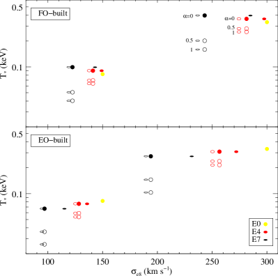
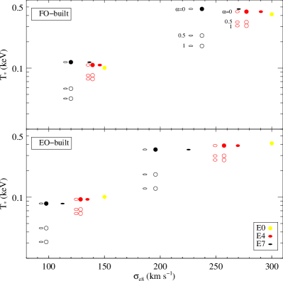
Figure 3: Distribution of $T_{*}$ for models derived from two spherical progenitors (yellow circles) of $\sigma_{\mathrm{e8}}=150$ or 300 $\mathrm{km\leavevmode\nobreak\ s}^{-1}$, with SIS (left panel) or Einasto DM halo (right panel). Colours refer to the intrinsic flattening of the descendants: E4 (red) and E7 (black). At given intrinsic flattening (i.e., at fixed colour), the shape of the symbols indicates the l.o.s. inclination: FO (circle) or EO view (ellipse). Filled symbols refer to $k=0$, empty symbols to $k=1$. Three values of $\alpha$ are considered ($\alpha=0,0.5,1$), as indicated for the FO-built sub-families of the $\sigma_{\mathrm{e8}}$=300 $\mathrm{km\leavevmode\nobreak\ s}^{-1}$ progenitor. When $k=1$, the increase of $\alpha$ decreases $T_{*}$ at any $\sigma_{\mathrm{e8}}$, from the value coincident with the non-rotating case ($k=0$) when $\alpha=0$, down to values that are lower for larger flattenings, when $\alpha=0.5$ and 1. In each sub-family, models with same intrinsic shape have the same $T_{*}$, independent of the FO or EO view, for fixed $(k,\alpha)$.

Figure 3 shows $T_{*}$ for various descendants of spherical progenitors with $\sigma_{\mathrm{e8}}=150$ and 300 $\mathrm{km\leavevmode\nobreak\ s}^{-1}$ (yellow circles), for two different DM haloes (SIS and Einasto in the left and right panels, respectively). As anticipated in Sect. 3.4, a major effect of flattening is the decrease of $\sigma_{\mathrm{e8}}$ of the descendants (with respect to the progenitor), that are then displaced on the left of their respective progenitor, in a way proportional to the flattening level (arrows in Fig. 1, see also Figs. 3 and 4).

The trend of $T_{*}$ with a pure change of shape in fully velocity dispersion supported models ($k=0$), is due to the specific flattening procedure (see Sect. 3.4). In the FO-built sub-families (Fig. 3, top panels), flatter models are more concentrated than rounder ones, while in the EO-built sub-families (bottom panels), they are more extended and diluted. Thus pure flattening produces a different effect on $T_{*}$: in the FO-built cases $T_{*}$ increases (as $T^{-}_{\mathrm{g}}$; see below), whereas in the EO-built cases $T_{*}$ decreases. Therefore, we conclude that real flat galaxies can be either more or less bound than spherical galaxies of the same mass, depending on their mass concentration. Overall, however, the variation in $T_{*}$ for both sub-families is not large: the maximum variation, from the progenitor to the E7 model, is an increase of $\sim 19$ percent for the FO-built cases, and a decrease of $\sim 18$ percent for the EO-built ones.

A larger effect on $T_{*}$ can instead be due to the presence of significant rotational support (empty symbols in Fig. 3), if not thermalised. In fact, when $k=1$, but $\alpha=0$ ($\gamma_{\mathrm{th}}=1$), the whole stellar kinetic energy, including the streaming one, is thermalised, and the $T_{*}$ values are coincident with those of the non-rotating case (full symbols), for the same galaxy shape. In the other cases of $\alpha\neq 0$, the rotational support always acts in the sense of reducing $T_{*}$, and the flatter the shape, the larger can be the reduction. The strongest reduction of $T_{*}$ is obtained for an isotropic rotator ($k=1$) E7 model, if the gas ejected from stars retains the same stellar streaming motion ($\alpha=1$, $\gamma_{\mathrm{th}}=0$): for the FO-built case, $T_{*}$ drops by $\sim 50$ percent with respect to the E0 model, and by $\sim 60$ percent with respect to the same E7 model with the ordered streaming motions fully thermalised ($\alpha=0$). For the EO-built case, $T_{*}$ drops by $\sim 70$ percent with respect to the E0 model, and by $\sim 60$ percent with respect to the same E7 model with $\alpha=0$. These percentages are obviously extreme values; the $T_{*}$ reduction is lower for milder flattenings, and for $k$ and $\alpha$ values smaller than 1. For a fixed galaxy shape, all possible $(k,\alpha)$ combinations fill a sort of triangular area on the $(\sigma_{\mathrm{e8}},T_{*})$ plane, identifiable by linking the symbols of a given $q$ (colour). Clearly, the rounder the galaxies, the weaker the effect of $k$ and, consequently, of $\alpha$ variations. All the above effects are independent of the galaxy luminosity (mass), and both the $\sigma_{\mathrm{e8}}=300$ and 150 $\mathrm{km\leavevmode\nobreak\ s}^{-1}$ families show the same (rescaled) behaviour in the $(\sigma_{\mathrm{e8}},T_{*})$ plane.

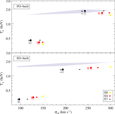
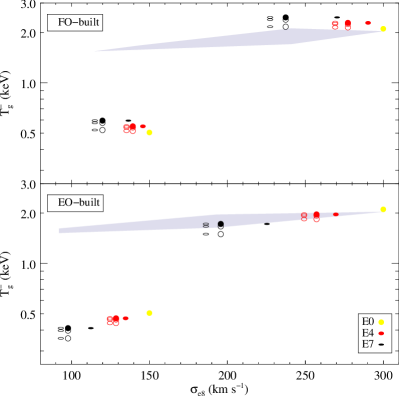
Figure 4: $T^{-}_{\mathrm{g}}$ for the same models in Fig. 3 (SIS and Einasto DM halo in the left and right panels, respectively); the same notation applies. The shaded area shows the range spanned by $T_{\mathrm{inj}}$, considering the variations in $T_{*}$ in Fig. 3, for $\eta=0.85$.

The trends described above are independent of the specific DM halo profile: models with an Einasto DM halo (right panel) show the same pattern as those with a SIS DM halo (left panel), just with a different normalisation due to the larger total DM content (see Table LABEL:tab:params). Similar results hold also for the Hernquist and NFW DM haloes.

In Fig. 4 we plot $T^{-}_{\mathrm{g}}$ for the same families in Fig. 3. Similarly to what happens for $T_{*}$, for fully velocity dispersion supported models, $T^{-}_{\mathrm{g}}$ gets larger with flattening for the FO-built sub-family ($\sim 21$ percent), while it decreases for the more diluted EO-built models ($\sim 12$ percent). Stellar streaming, when $\alpha>0$, acts in the sense of making the gas less bound, due to the centrifugal support of the injected gas, and then $T^{-}_{\mathrm{g}}$ decreases with increasing $\alpha$, at any fixed flat shape. This effect is maximum when $\alpha=1$ and the gas rotates as the stars. However, the decrease in $T^{-}_{\mathrm{g}}$ due to galaxy rotation is lower than obtained for $T_{*}$: for both sub-families, $T^{-}_{\mathrm{g}}$ drops at most by $\sim 13$ percent (for the E7 models), between the two extreme cases of $\alpha=0$ and $\alpha=1$. This produces that, in the FO-built case, $T^{-}_{\mathrm{g}}$ keeps always larger than for the progenitor when $q$ decreases, even for $k=\alpha=1$, while $T_{*}$ of rotating galaxies could become significantly lower than for the progenitor. Note that there are two compensating effects from stellar streaming when $\alpha\neq 0$: the stellar heating is lower than for $k=0$, but the gas is also less bound. Also these results are independent of the DM halo profile, as can be judged from the right panel of Fig. 4, that refers to the same models of the right panel of Fig. 3.

Since the flatter is the galaxy, the more it can be rotationally supported (and the more is rotationally supported, the larger is the effect of a corotating ISM), the effect of rotation is dependent on the degree of flattening, and thus it may prove difficult to disentangle observationally the two distinct effects due to shape and kinematics. On the theory side, we recall that a simplifying assumption made here is that $\boldsymbol{u}=\alpha\boldsymbol{v}$, and $\gamma_{\mathrm{th}}=(\alpha-1)^{2}$, while in reality the kinematical difference between stars and pre-existing gas may be more complex, as the extent of thermalisation; only numerical simulations will be able to establish what are the net effects on the gas evolution of stellar streaming motions (see Negri et al. 2013a, b).

Figure 4 finally shows the well known fact that the contribution from SNIa’s dominates the gas injection energy, since $T_{\mathrm{inj}}>>T_{*}$. This contribution (i.e., $T_{\mathrm{SN}}$) is independent of galaxy mass, which results into lower-mass models having $T^{-}_{\mathrm{g}}$ far lower than $T_{\mathrm{inj}}$, and $T^{-}_{\mathrm{g}}$ reaching $T_{\mathrm{inj}}$ for 200 $\mathrm{km\leavevmode\nobreak\ s}^{-1}\lesssim\sigma_{\mathrm{e8}}\lesssim 250$ $\mathrm{km\leavevmode\nobreak\ s}^{-1}$, depending on the DM profile. Galaxies with $\sigma_{\mathrm{e8}}\lesssim 200$ $\mathrm{km\leavevmode\nobreak\ s}^{-1}$ consequently are more prone to an outflow, and then to have a low hot gas content, as already suggested in the past by numerical simulations and by observations (CDPR, Sarazin et al. 2001; David et al. 2006; Pellegrini et al. 2007; Trinchieri et al. 2008). These findings are based on the assumption of a high thermalisation efficiency for SNIa’s ($\eta=0.85$), and the quoted $\sigma_{\mathrm{e8}}$ critical values become lower for lower $\eta$ values (as indicated by, e.g., Thornton et al. 1998), that decrease $T_{\mathrm{inj}}$. Variations in the dark matter may alter the $T^{-}_{\mathrm{g}}$ values, but small changes in $T^{-}_{\mathrm{g}}$ are found here for differences in the DM profile, and possible variations in the total DM amount cannot be very large, given the constraints from dynamical modelings within $R_{\mathrm{e}}$, and from cosmological simulations (taken into account here, Sect. 3.3). Indeed, the results for the Hernquist families are essentially identical to what we have shown for the Einasto halo, whereas for the NFW profile the trends are the same, but all the temperatures are shifted to higher values, due to their larger amounts of DM.

Table 3: Observed Properties of the ETG Sample with X-ray properties for the hot gas from Chandra observations.

Name	$d$	$\log(L_{\mathrm{K}})$	$k_{\mathrm{B}}T_{\mathrm{X}}$	$L_{\mathrm{X}}$	$V_{\mathrm{max}}$	$\sigma_{\mathrm{e8}}$	$V_{\mathrm{max}}/\sigma_{\mathrm{e8}}$	Ref.	Type	$q$
	(Mpc)	$(L_{\mathrm{K}\,\odot})$	(keV)	$(10^{40}\mathrm{erg\leavevmode\nobreak\ s}^{-1})$	$(\mathrm{km\leavevmode\nobreak\ s}^{-1})$	$(\mathrm{km\leavevmode\nobreak\ s}^{-1})$			RC3	2MASS
(1)	(2)	(3)	(4)	(5)	(6)	(7)	(8)	(9)	(10)	(11)
NGC 720	27.6	11.31	0.54	5.06	100	241	0.41	Binney et al. 1990	E5	0.55
NGC 821	24.1	10.94	0.15	2.13$\times 10^{-3}$	120	200	0.60	Coccato et al. 2009	E6?	0.62
NGC1023	11.4	10.95	0.32	6.25$\times 10^{-2}$	250	204	1.23	Noordermeer et al. 2008	SB0	0.38
NGC1052	19.4	10.93	0.34	4.37$\times 10^{-1}$	120	215	0.56	Milone et al. 2008	E4	0.70
NGC1316	21.4	11.76	0.60	5.35	150	230	0.65	Bedregal et al. 2006	SAB0	0.72
NGC1427	23.5	10.82	0.38	5.94$\times 10^{-2}$	45	171	0.26	D’Onofrio et al. 1995	cD	–
NGC1549	19.6	11.20	0.35	3.08$\times 10^{-1}$	40	210	0.19	Longo et al. 1994	E0-1	0.90
NGC2434	21.5	10.84	0.52	7.56$\times 10^{-1}$	20	205	0.10	Carollo et al. 1994	E0-1	0.98
NGC2768	22.3	11.23	0.34	1.26	195	205	0.95	Proctor et al. 2009	E6	0.46
NGC3115	9.6	10.94	0.44	2.51$\times 10^{-2}$	260	239	1.09	Fisher 1997	S0	0.39
NGC3377	11.2	10.45	0.22	1.17$\times 10^{-2}$	97	144	0.67	Simien et al. 2002	E5-6	0.58
NGC3379	10.5	10.87	0.25	4.69$\times 10^{-2}$	60	216	0.28	Weijmans et al. 2009	E1	0.85
NGC3384	11.5	10.75	0.25	3.50$\times 10^{-2}$	150	161	0.93	Fisher 1997	SB0	0.51
NGC3585	20.0	11.25	0.36	1.47$\times 10^{-1}$	200	198	1.01	Fisher 1997	E6	0.63
NGC3923	22.9	11.45	0.45	4.41	31	250	0.12	Norris et al. 2008	E4-5	0.64
NGC4125	23.8	11.35	0.41	3.18	150	227	0.66	Pu et al. 2010	E6 pec	0.63
NGC4261	31.6	11.43	0.66	7.02	50	300	0.17	Bender et al. 1994	E2-3	0.86
NGC4278	16.0	10.87	0.32	2.63$\times 10^{-1}$	60	252	0.24	Bender et al. 1994	E1-2	0.93
NGC4365	20.4	11.30	0.44	5.12$\times 10^{-1}$	80	245	0.33	Surma et al. 1995	E3	0.74
NGC4374	18.3	11.37	0.63	5.95	60	292	0.21	Coccato et al. 2009	E1	0.92
NGC4382	18.4	11.41	0.40	1.19	70	187	0.37	Fisher 1997	SA0	0.67
NGC4472	16.2	11.60	0.80	18.9	73	294	0.25	Fisher et al. 1995	E2	0.81
NGC4473	15.7	10.86	0.35	1.85$\times 10^{-1}$	70	192	0.36	Emsellem et al. 2004	E5	0.54
NGC4526	16.9	11.20	0.33	3.28$\times 10^{-1}$	246	232	1.06	Pellegrini et al. 1997	SAB0	0.43
NGC4552	15.3	11.01	0.52	2.31	17	268	0.06	Krajnović et al. 2008	E0-1	0.94
NGC4621	18.2	11.16	0.27	6.08$\times 10^{-1}$	140	225	0.62	Bender et al. 1994	E5	0.65
NGC4649	16.8	11.49	0.77	11.7	120	315	0.38	Pinkney et al. 2003	E2	0.81
NGC4697	11.7	10.92	0.33	1.91$\times 10^{-1}$	115	174	0.66	De Lorenzi et al. 2008	E6	0.63
NGC5866	15.3	10.95	0.35	2.42$\times 10^{-1}$	210	159	1.32	Neistein et al. 1999	SA0	0.42

Finally we comment on the preliminary investigation about the role of flattening and rotation on the global energetics of the ISM in CP96. They built fully analytical axisymmetric two-component galaxy models, where the stellar and dark mass distributions were described by the Miyamoto–Nagai potential-density pair. They varied the shape of both the stellar component and the dark matter halo from flat to spherical, and the amount of azimuthal ordered motions through the Satoh $k$-decomposition. Their conclusion was that, for quite round systems, flattening can have a substantial effect in reducing the binding energy of the hot gas, contrary to galaxy rotation that seemed to have a negligible role. The opposite was suggested for very flat systems. These results were confirmed by 2D hydrodynamical simulations (D’Ercole & Ciotti, 1998). We stress here that the models in CP96, while capturing the main effects of flattening and rotation on the global energetics of the hot haloes of ETGs, were not tailored to reproduce in detail the observed properties of real ETGs. Our current findings, based on more realistic galaxy models, reveal a more complicated situation, where the flattening importance on the ISM status is mediated by the amount of rotation and its specific thermalisation history. Remarkably enough, however, when flattening a two-component Miyamoto–Nagai model following the same procedure here adopted (constant $M_{*}$, $R_{\mathrm{e}}$ and $M_{\mathrm{h}}$), its $T^{-}_{\mathrm{g}}$ remains close to that of its spherical progenitor (i.e., the model moves almost parallel to the solid lines in fig. 2 in CP96).

4.2 Comparison with observed ETGs properties in the X-rays

Now we compare our estimates for $T_{*}$ and $T^{-}_{\mathrm{g}}$ with observed temperatures $T_{\mathrm{X}}$ and gas content, respectively, for the BKF sample. Observed X-ray and $K$-band luminosities, central stellar velocity dispersions, rotation velocities, and galaxy shape are given in Tab. LABEL:tab:ETGs. Figure 5 shows observed (points) and model temperatures (lines) versus $L_{\mathrm{K}}$, with $T_{\mathrm{X}}$ plotted with a different colour reflecting the ETG shape and rotational support. In order to make the comparison between models and observations more consistent, the $L_{\mathrm{K}}$ of the models have been calculated using the mean $L_{\mathrm{K}}/L_{\mathrm{V}}=3.4$ of the ETGs in this sample. When comparing observed and model temperature values at fixed $L_{\mathrm{K}}$, the mass is the same for all the models, and it should be roughly so also for the observed ETGs. At fixed $L_{\mathrm{K}}$, then, the $T_{*}$ variation due to shape and stellar streaming is obtained from all the $T_{*}$ values of the descendants of a progenitor (we consider the Einasto models of Fig. 3), regardless of the FO or EO view. When comparing observed and model temperatures as a function of $\sigma_{\mathrm{e8}}$ instead, at any $\sigma_{\mathrm{e8}}$ the mass could be different. Figure 5 shows again how the effect of rotation can be potentially stronger than that of shape (as already indicated by Fig. 3): moderately larger or smaller $T_{*}$ can be produced by flattening, depending on the way it is realized, while $T_{*}$ can be much lowered by galactic rotation. Thus, at fixed $L_{\mathrm{K}}$, the largest variation in $T_{*}$ with respect to the spherical case (yellow line) does not come from a variation of shape, but is a decrease of $T_{*}$ due to rotation with $\alpha=1$ (no thermalisation).

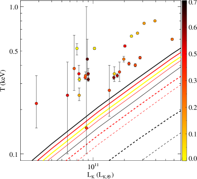
Figure 5: $T_{*}$ (lines) for all the progenitors in Tab. LABEL:tab:params with the Einasto halo, and their descendants (with $\alpha=0$ or $\alpha=1$), and the observed $T_{\mathrm{X}}$ (circles), for the ETGs in the BKF sample, as a function of $L_{\mathrm{K}}$. The yellow line refers to the progenitor ETGs, the red lines to the E4 shape, the black ones to the E7 shape; lines are solid for $k=0$, and dashed for $k=1$ and $\alpha=1$. For each colour, lines representing the case of $k=1$ and $\alpha=0$ are coincident with the solid lines. Thick and thin lines refer to the FO and EO-built models, respectively. Left panel: the colour-coding for the observed ETGs indicates their ellipticity $\epsilon=1-q$, as measured in the Ks-band, from 2MASS (see Tab. LABEL:tab:ETGs), and is calibrated as for the previous figures [i.e., to be yellow for the E0 ($q=1,\epsilon=0$), red for the E4 ($q=0.6,\epsilon=0.4$), and black for the E7 ($q=0.3,\epsilon=0.7$); see the colour bar on the right for the $\epsilon$ of the other colours]. Right panel: the colour-coding indicates the rotational support $V_{\mathrm{max}}/\sigma_{\mathrm{e8}}$. Note that, for an EO view, the models of the dashed lines would have $V_{\mathrm{max}}/\sigma_{\mathrm{e8}}=0.90-0.95$ for the E4 case, and $V_{\mathrm{max}}/\sigma_{\mathrm{e8}}=1.5-1.6$ for the E7 case.

In Fig. 5 all $T_{\mathrm{X}}$ are larger than $T_{*}$, yet much closer to $T_{*}$ than to $T_{\mathrm{inj}}\sim 1.5-2$ keV (see Fig. 4). This may be evidence of two facts: either the SNIa’s thermalisation $\eta$ is low, or the gas flows establish themselves at a temperature close to the virial temperature of the galaxy, and most of the SNIa’s input is spent in cooling (in gas-rich ETGs), or in lifting the gas from the potential well, and imparting bulk velocity to the outflowing gas (in gas-poorer ETGs; see P11 for a quantification of these effects, and Tang et al. 2009 and Li et al. 2011a for addressing also other solutions to this problem). A combination of the two explanations may also be at place, of course. In any case, the proximity of the observed $T_{\mathrm{X}}$ values to $T_{*}$ provides an empirical evidence of the importance of the study of $T_{*}$ and its variations; it would not have been so, if we had found $T_{\mathrm{X}}$ to be closer to $T_{\mathrm{inj}}$.

Going now into the question of whether possible effects from shape and stellar streaming are apparent on $T_{\mathrm{X}}$, Fig. 5 shows a mild indication that flatter shapes and more rotationally supported ETGs tend to show a lower $T_{\mathrm{X}}$, with respect to rounder, less rotating ETGs. This is similar to the recent result by S13, that fast rotators seem to be confined to lower temperatures than slow rotators. S13 suggested that in ETGs with a larger degree of rotational support, the kinetic energy associated with the stellar ordered motions may be thermalised less efficiently. Preliminary results of hydrodynamical simulations seem to indicate that this is the case (Negri et al., 2013a, b). Based on the analysis of Sect. 4.1, we can propose an explanation for the trends in Fig. 5 that seems consistent with the present data, and that represents a prediction for when the sample in Fig. 5, still quite small, will be hopefully enlarged: stellar streaming always reduces $T_{*}$, in a way proportional to $k$ and $\alpha$, up to an amount that can be as large as 60 percent, while flattening itself is less important (though necessary for rotation to be important).

We now move to consider possible effects from shape and rotation on the gas content, starting from the hypothesis that it is linked to the relative size of $T^{-}_{\mathrm{g}}$ and $T_{\mathrm{inj}}$. Figure 6 shows the observed $L_{\mathrm{X}}$ values, together with the energies (referring to the mass of gas injected in the unit time) describing the stellar heating $L_{*}$, the SNIa’s heating $L_{\mathrm{SN}}$, and the requirement for escape $L^{-}_{\mathrm{g}}$. All quantities are normalised to $L_{\mathrm{K}}$, and are computed using the expression for the stellar mass loss rate $\dot{M}_{*}$ and the temperatures defined in Sect. 2, such that $L^{-}_{\mathrm{g}}=\dot{M}_{*}E^{-}_{\mathrm{g}}=3k_{\mathrm{B}}\dot{M}_{*}T^{-}_{\mathrm{g}}/(2\mu m_{\mathrm{P}})$, $L_{*}=3k_{\mathrm{B}}\dot{M}_{*}T_{*}/(2\mu m_{\mathrm{P}})$, and $L_{\mathrm{SN}}=\eta E_{\mathrm{SN}}R_{\mathrm{SN}}$. Figure 6 clearly shows that flatter and more rotationally supported ETGs tend to have a lower $L_{\mathrm{X}}/L_{\mathrm{K}}$, as already known (see Sect. 1).

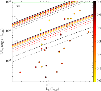
Figure 6: Comparison between the run of various luminosities vs. $L_{\mathrm{K}}$, for all the progenitors in Tab. LABEL:tab:params (Einasto halo case) and a selection of their descendants (only cases of $\alpha=0,1$), and for the observed $L_{\mathrm{X}}$ for the ETGs in the BKF sample; all quantities are normalised to $L_{\mathrm{K}}$. The lower group of lines gives $L_{*}/L_{\mathrm{K}}$, the upper one gives $L^{-}_{\mathrm{g}}/L_{\mathrm{K}}$, the horizontal line is $L_{\mathrm{SN}}/L_{\mathrm{K}}$ for $\eta=0.85$. The yellow line refers to the progenitor ETGs, the red lines to the E4 shape, the black ones to the E7 shape; lines are solid for $k=0$, and dashed for $k=1$ and $\alpha=1$, respectively. Thick and thin lines refer to the FO and EO-built models, respectively. The colour-coding for the observed ETGs indicates their ellipticity $\epsilon=1-q$ (left panel) and the rotational support $V_{\mathrm{max}}/\sigma_{\mathrm{e8}}$ (right panel), and is calibrated as for the previous Fig. 5.

As shown in Sect. 4.1, however, the effect of shape or rotation on $L^{-}_{\mathrm{g}}$ is small, so we cannot claim an important direct role for these two major galactic properties on determining a lower gas content and then $L_{\mathrm{X}}$. It has been suggested that a possible indirect effect could come from galactic rotation if it is effective in creating a gas disc, where gas cooling is triggered, the temperature is lowered, and then $L_{\mathrm{X}}$ is reduced (Brighenti & Mathews, 1997). Other possibilities may be related to global instabilities of rotating flows, perhaps associated with inefficient thermalisation (Negri et al., 2013b). Note that the X-ray emissivity is also dependent on the gas temperature, and one could think that the lower $L_{\mathrm{X}}$ of flat/rotating ETGs could be due to having these preferentially a lower $T_{\mathrm{X}}$ (Fig. 5). This cannot be the explanation, though, because the emissivity in the 0.3-8 keV band decreases very mildly with decreasing temperature, for temperatures below a value of $\sim 1$ keV. Another explanation for a lower $L_{\mathrm{X}}/L_{\mathrm{K}}$ could be a lower stellar age in fast rotators: indeed, S13 found that molecular gas and young stellar populations are detected only in fast rotators across the entire ATLAS^3D sample, and a younger age is known to be linked to a lower $L_{\mathrm{X}}$ (BKF, O’Sullivan et al. 2001).

Also, note in Fig. 6 how there are many ETGs with $L_{\mathrm{X}}$ lower than $L_{*}$: they do not even radiate $L_{*}$. For them, the outflow must be very important, and must have employed almost all of $L_{\mathrm{SN}}$. Numerical simulations (CDPR) have already shown that $L_{\mathrm{X}}$ can be even lower than $L_{*}$ during winds/outflows. As $L^{-}_{\mathrm{g}}$ increases and becomes closer to $L_{\mathrm{SN}}$, the ETGs below $L_{*}$ disappear.

Finally, BKF found a positive correlation between $L_{\mathrm{X}}$ and $T_{\mathrm{X}}$, valid down to the gas-poor galaxies, that on average have the shallowest potentials ($L_{\mathrm{K}}\lesssim 2\times 10^{11}L_{\mathrm{K}\,\odot}$ and $\sigma_{\mathrm{e8}}\lesssim$ 200 $\mathrm{km\leavevmode\nobreak\ s}^{-1}$) and are expected to host outflows; also in the $L_{\mathrm{X}}-L_{\mathrm{K}}$ plot, in the large variation in $L_{\mathrm{X}}$ at any $L_{\mathrm{K}}\gtrsim 7\times 10^{10}L_{\mathrm{K}\,\odot}$, ETGs with the lowest $L_{\mathrm{X}}$ tend to be the coldest ones. This seemed a puzzle, if outflows (lower $L_{\mathrm{X}}$) are expected to be hotter than inflows (large $L_{\mathrm{X}}$). P11 re-examined the $T_{\mathrm{X}}$ behavior, considering $T_{\mathrm{X}}$ values rescaled by $T_{*}$, where for the latter the case of a spherical galaxy with an isotropic velocity dispersion tensor was taken. The gas of ETGs with $\sigma_{\mathrm{e8}}\lesssim$ 200 $\mathrm{km\leavevmode\nobreak\ s}^{-1}$ turned out to be colder in an absolute sense, but to have the largest values for the rescaled $T_{\mathrm{X}}$; the latter also tend to the (rescaled) $T_{\mathrm{esc}}^{\mathrm{sub}}$, a fiducial average temperature of gas in outflow (Sect. 2.2), consistent with the expectation for the gas flow status of these ETGs. At intermediate $\sigma_{\mathrm{e8}}$ values, though (200 $\mathrm{km\leavevmode\nobreak\ s}^{-1}<\sigma_{\mathrm{e8}}<250$ $\mathrm{km\leavevmode\nobreak\ s}^{-1}$), still the rescaled $T_{\mathrm{X}}$ seemed to be lower for the gas poorest ETGs, which remained unexplained. Can we suggest that at these intermediate $\sigma_{\mathrm{e8}}$ the effect of shape or rotation is responsible for a decrease of both $T_{\mathrm{X}}$ and $L_{\mathrm{X}}$? And then, when normalising $T_{\mathrm{X}}$ by a $T_{*}$ appropriate for the shape and rotational level of the host galaxy, the result is larger than when normalising by the $T_{*}$ of a spherical ETG of same $\sigma_{\mathrm{e8}}$?

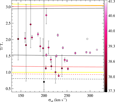
Figure 7: Relative temperatures versus $\sigma_{\mathrm{e8}}$ for observed ETGs and models (only EO-built models observed EO; the plot is very similar for the FO-built models). The colours and linetype for the models are the same as in Fig. 5. $T_{*}$ values (lower bundle of lines) are normalised to $T_{*}$ corresponding to a spherical galaxy with an isotropic velocity tensor (given by the yellow line in Fig. 5); $T_{\mathrm{esc}}^{\mathrm{sub}}$ (upper bundle of lines) and $T_{\mathrm{X}}$’s are normalised to the $T_{*}$ of the corresponding shape (neglecting rotation). In particular, observed ETGs with $q$ in the range [1,0.75] are normalised to $T_{*}$ of the E0 model, those with $q$ in the range [0.75,0.45] are normalised to $T_{*}$ of the E4 model, whereas those with $q<0.45$ are normalised to $T_{*}$ of the E7 model. The colour-coding for the observed ETGs indicates their log$L_{\mathrm{X}}$($\mathrm{erg\leavevmode\nobreak\ s}^{-1}$), in the left panel, and the rotational support $V_{\mathrm{max}}/\sigma_{\mathrm{e8}}$, in the right panel, as indicated by the colour bar on the right.

Figure 7 shows $T_{\mathrm{X}}$ values normalised by a $T_{*}$ appropriate for the apparent shape of the galaxy, neglecting rotation; it confirms that at low $\sigma_{\mathrm{e8}}$ the gas is relatively hotter, and reaches close to $T_{\mathrm{esc}}^{\mathrm{sub}}/T_{*}$ (P11). In the right panel, the colour indicates the level of rotational support $V_{\mathrm{max}}/\sigma_{\mathrm{e8}}$; if rotation is not neglected, in this plot the properly normalised $T_{\mathrm{X}}$ of rotating ETGs would become higher (see, e.g., Fig. 5). Indeed, in the intermediate $\sigma_{\mathrm{e8}}$ region, some of the gas-poor ETGs with the lowest $T_{\mathrm{X}}/T_{*}$, are also highly rotating, and then their position in the plot would be higher, thus at least partially accounting for the segregation.

5 Summary and conclusions

In this paper we investigated the relationship between the temperature and luminosity of the hot X-ray emitting haloes of ETGs and the galactic shape and rotational support. This work is an extension of previous similar studies (CP96, Pellegrini et al. 1997, P11).

By solving the Jeans equations, we built a large set of axisymmetric three-component (stars, dark matter halo, SMBH) galaxy models, representative of observed ETGs. We varied the degree of flattening and rotational support of the stellar component, in order to establish what is the dependence of the temperature and binding energy of the injected gas on the observed galaxy shape and internal kinematics. For the injected gas, we defined the equivalent temperature of stellar motions as $T_{*}=T_{\sigma}+\gamma_{\mathrm{th}}T_{\mathrm{rot}}$, where the parameter $\gamma_{\mathrm{th}}$ takes into account how much of the ordered rotation of the galaxy is eventually thermalised by the stellar mass losses. We considered the simplified case in which the pre-existing gas velocity is proportional to the stellar streaming velocity. When pre-existing gas and stars rotate with the same velocity, no ordered stellar kinetic energy is thermalised ($\gamma_{\mathrm{th}}=0$); when the gas is at rest, all the kinetic energy due to stellar streaming is thermalised ($\gamma_{\mathrm{th}}=1$). We also defined the temperature equivalent ($T^{-}_{\mathrm{g}}$) to the binding energy for the injected gas. Our main results are as follows:

• The major effect of flattening the stellar component of a spherical ETG is a decrease of the observed $\sigma_{\mathrm{e8}}$ value of its flatter counterparts of same mass and same circularized $R_{\mathrm{e}}$. This decrease is proportional to the flattening level and depends also on the viewing angle. For each shape, in velocity dispersion supported models, the decrease is larger for the FO-view and smaller for the EO-view, and it reaches $\sim 35$ percent for the E7 shape seen FO. In isotropic rotators, the decrease is instead larger for the EO view. Thus, ETGs with the same roundish appearance and the same observed $\sigma_{\mathrm{e8}}$ may have a significantly different mass. This finding raises the issue of the reliability of the use of $\sigma_{\mathrm{e8}}$ as a proxy for the dynamical mass of an ETG, a point particularly relevant for studies of the hot haloes properties, that mainly depend on the galaxy mass.

• Flatter models can be either more or less concentrated than rounder ones of the same mass and same circularized $R_{\mathrm{e}}$, depending on how they are built: if $R_{\mathrm{e}}$ is kept constant for a FO view, flatter models are more concentrated and bounded than the round counterpart; the opposite is true if $R_{\mathrm{e}}$ is kept constant for an EO view. As a consequence, the effect of a pure change of shape is an increase of $T_{*}$ and $T^{-}_{\mathrm{g}}$ in the first way of flattening, and a decrease in the second one. Overall, however, the variation in $T_{*}$ for both cases is mild, within $\sim 20$ percent even for the maximum degree of flattening (the E7 model). Similarly, $T^{-}_{\mathrm{g}}$ gets larger by at most $\sim 20$ percent, and decreases by at most $\sim 12$ percent.

• A more significant effect on $T_{*}$ can be due to the amount of rotational support. The isotropic rotator case is investigated here ($k=1$). If $\gamma_{\mathrm{th}}=1$, the whole stellar kinetic energy, including the streaming one, is thermalised, and $T_{*}$ coincides with that of the non-rotating case, for the same galaxy shape. If $\gamma_{\mathrm{th}}<1$, $T_{*}$ is instead always reduced, and the larger so the flatter is the shape. The strongest reduction is obtained for the E7 models when $\gamma_{\mathrm{th}}=0$, and then $T_{*}$ can drop by $50-70$ percent with respect to the E0 models. Thus, the presence of stellar streaming, when not thermalised, acts always in the sense of decreasing $T_{*}$, and the size of this decrease depends on the relative motion between pre-existing gas and stars. Clearly, the flatter the galaxies, the stronger can be the rotational support, and, consequently its potential effect on $T_{*}$. Thus the effect of rotation is dependent on the degree of flattening, and, as a minimum, it requires a flat shape as a premise.

• Since stellar streaming acts in the sense of making the gas less bound due to the centrifugal support, at any fixed galaxy shape and rotational support $T^{-}_{\mathrm{g}}$ decreases in proportion to how the velocity field of the ISM is close to that of the stars. However, this decrease is lower than that produced on $T_{*}$: $T^{-}_{\mathrm{g}}$ drops at most by $\sim 13$ percent (for the E7 models), between the two extreme cases of ISM at rest and gas rotating as the stars. Note then two compensating effects from stellar streaming when $\gamma_{\mathrm{th}}<1$: $T_{*}$ is lower than for a non-rotating galaxy, but the gas is also less bound.

• All the above trends and effects are independent of the galaxy luminosity (mass), and dark halo shape. Only the normalization of $T_{*}$ and $T^{-}_{\mathrm{g}}$ changes, if the dark halo mass changes (e.g., it increases from the SIS to the Einasto to the Hernquist to the NFW halo models).

The comparison of the above results with observed $T_{\mathrm{X}}$ and $L_{\mathrm{X}}$ for the ETGs in the Chandra sample of BKF shows that:

• All observed $T_{\mathrm{X}}$ are larger than $T_{*}$, but much closer to $T_{*}$ than to $T_{\mathrm{SN}}$. $T_{*}$ ranges between 0.1 and 0.4 keV, for 150 $\mathrm{km\leavevmode\nobreak\ s}^{-1}\lesssim\sigma_{\mathrm{e8}}\lesssim 300$ $\mathrm{km\leavevmode\nobreak\ s}^{-1}$ (the lower end being possibly even lower, depending on the effects of rotation), while $T_{\mathrm{SN}}\approx 1.5$ keV (for a thermalisation parameter $\eta=0.85$), so that the contribution from SNIa’s dominates the gas injection energy ($T_{\mathrm{inj}}\sim 1.5-2$ keV), that is then practically insensitive to changes in $T_{*}$ due to the galaxy shape or kinematics. The proximity of the observed $T_{\mathrm{X}}$ values to $T_{*}$ indicates that $\eta$ may be lower, and/or that the gas tends to establish itself at a temperature close to the virial temperature, in all flow phases. In any case, this proximity provides an empirical confirmation of the relevance of a study of $T_{*}$ and its variations.

• For 200 $\mathrm{km\leavevmode\nobreak\ s}^{-1}\lesssim\sigma_{\mathrm{e8}}\lesssim 250$ $\mathrm{km\leavevmode\nobreak\ s}^{-1}$, $T^{-}_{\mathrm{g}}$ becomes larger than $T_{\mathrm{inj}}$, and inflows in these galaxies can become important. These $\sigma_{\mathrm{e8}}$ values could be lower if $\eta<0.85$, and if the dark matter amount is larger than assumed here. Galaxies with $\sigma_{\mathrm{e8}}\lesssim 200$ $\mathrm{km\leavevmode\nobreak\ s}^{-1}$ ($L_{\mathrm{K}}\lesssim 2\times 10^{11}L_{\mathrm{K}\,\odot}$), instead have a high probability of hosting an outflow, and then a low hot gas content, as confirmed by observations of $L_{\mathrm{X}}/L_{\mathrm{K}}$ vs. $L_{\mathrm{K}}$. The ratio $L_{\mathrm{X}}/L_{\mathrm{K}}$ seems to be lower also for a flatter shape and larger rotation. However, the effect of shape or rotation on $T^{-}_{\mathrm{g}}$ is small, thus these two major galactic properties are not expected to play an important direct role in determining the gas content. Indirect effects may be more likely (as galactic rotation triggering large-scale instabilities in the gas, or the lower age of fast rotators). For many ETGs, $L_{\mathrm{X}}/L_{\mathrm{K}}$ is much lower than $L_{*}/L_{\mathrm{K}}$, indicating clearly the presence of an outflow.

• We find a mild indication that, at fixed $L_{\mathrm{K}}$, flatter shapes and more rotationally supported ETGs show a lower $T_{\mathrm{X}}$, with respect to rounder, less rotating ETGs (similarly to what recently found by S13). This tendency can be easily explained by the effects predicted here on $T_{*}$ due to flattening and rotation. Since, for a fixed galaxy mass, a decrease of $T_{*}$ due to rotation is predicted to be potentially stronger than produced by shape without rotation, we propose that not thermalised stellar streaming is a more efficient cause of the (possibly) lower $T_{\mathrm{X}}$.

• Extending a P11 result, we find that, when rescaled by a $T_{*}$ value representative of a fully velocity dispersion supported ETG of the corresponding shape, the $T_{\mathrm{X}}/T_{*}$ values of outflows (at $\sigma_{\mathrm{e8}}\lesssim 200$ $\mathrm{km\leavevmode\nobreak\ s}^{-1}$) are larger than those of inflows (at $\sigma_{\mathrm{e8}}\gtrsim 250$ $\mathrm{km\leavevmode\nobreak\ s}^{-1}$). At 200 $\mathrm{km\leavevmode\nobreak\ s}^{-1}\lesssim\sigma_{\mathrm{e8}}\lesssim 250$ $\mathrm{km\leavevmode\nobreak\ s}^{-1}$, where the $T_{\mathrm{X}}/T_{*}$ values seem to be lower for the gas poorest ETGs, part of the trend could be explained by a few of these ETGs being highly rotating. Note that the observed galactic rotation depends on the viewing angle at which these low $T_{\mathrm{X}}$ and low $L_{\mathrm{X}}$ ETGs are seen, thus it is difficult to find a clear indication of a systematic trend in the data.

As a necessary parallel investigation, we are going to perform 2D hydrodynamical simulations to explore the actual behaviour of the ISM for the models here studied (Negri et al., 2013b). The goal will be to establish, as a function of galactic structure and kinematics, the presence of major hydrodynamical instabilities, the efficiency of thermalisation of stellar streaming motions, and their impact on $T_{\mathrm{X}}$ and $L_{\mathrm{X}}$.

Appendix A The fluid equations in the presence of source terms

The equations of fluid dynamics in the presence of different sources of mass, momentum and energy, under the simplifying assumption of isotropy of the mass losses, can be written (D’Ercole et al., 2000) as

$$\dfrac{D\rho}{Dt}+\rho(\nabla\cdot\boldsymbol{u})=\mathscr{M},$$ (24)

$$\rho\dfrac{D\boldsymbol{u}}{Dt}=-\rho\nabla\Phi-\nabla p+\mathscr{M}(\boldsymbol{v}-\boldsymbol{u}),$$ (25)

$$\begin{split}\dfrac{DE}{Dt}+(E+p)\nabla\cdot\boldsymbol{u}=&\,\Sigma\mathscr{M}_{i}\left[e_{i}+\dfrac{u_{\mathrm{s},\,i}^{2}}{2}\right]-\mathscr{L}\\ &+\dfrac{\mathscr{M}}{2}\left[\Arrowvert\boldsymbol{u}-\boldsymbol{v}\Arrowvert^{2}+\text{Tr}(\boldsymbol{\sigma}^{2})\right].\end{split}$$ (26)

Here $\mathscr{M}(\mathbf{x},t)=\Sigma\mathscr{M}_{i}$ is the total mass return per unit time and volume, due to different sources (e.g., stellar winds and SNIa events) associated with a stellar population with streaming velocity $\boldsymbol{v}(\mathbf{x},t)$ and velocity dispersion $\boldsymbol{\sigma}^{2}(\mathbf{x},t)$. $e_{i}(\mathbf{x},t)$ is the internal energy return per unit mass and time of the $i$-th source field, and $u_{\mathrm{s},\,i}(\mathbf{x},t)$ is the modulus of the relative velocity of the material injected by the $i$-th source field with respect to the source star. Finally, $\mathscr{L}$ are the bolometric radiative losses per unit time and volume.

For example, in applications as the one in this paper, $\mathscr{M}$ is represented by the sum of stellar winds and SNIa explosions ejecta. Often, $e_{\mathrm{wind}}$ and $u_{\mathrm{s,wind}}$ are neglected, being significantly smaller than the contribution of $\text{Tr}(\boldsymbol{\sigma}^{2})$, while the opposite holds for SNIa events, where $\mathscr{M}_{\mathrm{SN}}\text{Tr}(\boldsymbol{\sigma}^{2})$ is negligible with respect to the energy injection due to the SNIa explosions. In our case, $\gamma_{\mathrm{th}}$ in Eq. (5) derives from the full mass injection term in Eq. (26), where both contributions are taken into account.

Appendix B The code

All the relevant dynamical properties of the models are computed using a numerical code built on purpose (Posacki et al., 2013; Posacki, 2011). Starting from an axisymmetric density distribution the code computes in terms of elliptic integrals the associated gravitational potential and vertical and radial forces. The code then solves the Jeans equations in cylindrical coordinates $(R,z,\varphi)$. For an axisymmetric density distribution $\rho_{*}(R,z)$ supported by a two-integral phase-space distribution function (DF), the Jeans equations write

$$\dfrac{\partial\rho_{*}\sigma^{2}}{\partial z}=-\rho_{*}\dfrac{\partial\Phi_{\mathrm{tot}}}{\partial z},$$ (27)

and

$$\dfrac{\partial\rho_{*}\sigma^{2}}{\partial R}+\rho_{*}\dfrac{\sigma^{2}-\overline{v_{\varphi}^{2}}}{R}=-\rho_{*}\dfrac{\partial\Phi_{\mathrm{tot}}}{\partial R},$$ (28)

(e.g. Binney & Tremaine 1987), where $\Phi_{\mathrm{tot}}$ is the sum of the gravitational potentials of all the components (e.g. stars, dark halo, black hole). As well known, for a two-integral DF (1) the velocity dispersion tensor is diagonal and aligned with the coordinate system; (2) the radial and vertical velocity dispersions are equal, i.e. $\sigma_{R}=\sigma_{z}\equiv\sigma$; (3) the only non-zero streaming motion is in the azimuthal direction.

In order to control the amount of ordered azimuthal velocity $\overline{v_{\varphi}}$, we adopted the $k$-decomposition introduced by Satoh (1980)

$$\overline{v_{\varphi}}^{2}=k^{2}(\overline{v_{\varphi}^{2}}-\sigma^{2}),$$ (29)

and then it follows

$$\sigma_{\varphi}^{2}\equiv\overline{v_{\varphi}^{2}}-\overline{v_{\varphi}}^{2}=\sigma^{2}+(1-k^{2})(\overline{v_{\varphi}^{2}}-\sigma^{2}),$$ (30)

where $0\leqslant k\leqslant 1$. The case $k=1$ corresponds to the isotropic rotator, while for $k=0$ no net rotation is present and all the flattening is due to the azimuthal velocity dispersion $\sigma_{\varphi}$. In principle, $k$ can be a function of $(R,z)$, and so more complicated (realistic) velocity fields can be realized (CP96; see also Negri et al. 2013a). The code then projects all the relevant kinematical fields, together with the stellar density.

The projections along a general l.o.s. of the stellar density $\rho_{*}$, streaming velocity $\boldsymbol{v}$ and velocity dispersion tensor $\boldsymbol{\sigma}^{2}$ are

$$\Sigma_{*}=\int_{-\infty}^{+\infty}\rho_{*}dl,$$ (31)

$$\Sigma_{*}v_{\mathrm{los}}=\int_{-\infty}^{+\infty}\rho_{*}\langle{\boldsymbol{v},\boldsymbol{n}}\rangle dl,$$ (32)

$$\Sigma_{*}\sigma^{2}_{\mathrm{P}}=\int_{-\infty}^{+\infty}\rho_{*}\langle{\boldsymbol{\sigma}^{2}\boldsymbol{n},\boldsymbol{n}}\rangle dl,$$ (33)

respectively, where $\langle{,}\rangle$ is the scalar product, $\boldsymbol{n}$ is the l.o.s. direction and $l$ is the integration path along $\boldsymbol{n}$. Note that if a rotational support is present, then $\sigma^{2}_{\mathrm{P}}$ is not the l.o.s. (i.e. the observed) velocity dispersion $\sigma_{\mathrm{los}}^{2}$, given by

$$\sigma^{2}_{\mathrm{los}}=\sigma_{\mathrm{P}}^{2}+V_{\mathrm{P}}^{2}-v_{\mathrm{los}}^{2},$$ (34)

where $V_{\mathrm{P}}^{2}$ is the projection of $\langle{\boldsymbol{n},\boldsymbol{v}}\rangle^{2}$ (CP96). In particular, the face-on projections are

$$\Sigma_{*}=2\int_{0}^{\infty}\rho_{*}dz,$$ (35)

$$\Sigma_{*}\sigma^{2}_{\mathrm{P}}=2\int_{0}^{\infty}\rho_{*}\sigma^{2}dz,$$ (36)

with $\sigma^{2}_{\mathrm{los}}=\sigma^{2}_{\mathrm{P}}$. The edge-on projections are instead

$$\Sigma_{*}=2\int_{R}^{\infty}\dfrac{\rho_{*}\tilde{R}\,d\tilde{R}}{\sqrt{\tilde{R}^{2}-R^{2}}},$$ (37)

$$\Sigma_{*}v_{\mathrm{los}}=2R\int_{R}^{\infty}\dfrac{\rho_{*}\overline{v_{\varphi}}\,d\tilde{R}}{\sqrt{\tilde{R}^{2}-R^{2}}},$$ (38)

$$\Sigma_{*}\sigma_{\mathrm{P}}^{2}=2\int_{R}^{\infty}\left[(\tilde{R}^{2}-R^{2})\sigma^{2}+R^{2}\sigma^{2}_{\varphi}\right]\dfrac{\rho_{*}\,d\tilde{R}}{\tilde{R}\sqrt{\tilde{R}^{2}-R^{2}}},$$ (39)

$$\Sigma_{*}V_{\mathrm{P}}^{2}=2R^{2}\int_{R}^{\infty}\dfrac{\rho_{*}\overline{v_{\varphi}}^{2}\,d\tilde{R}}{\tilde{R}\sqrt{\tilde{R}^{2}-R^{2}}},$$ (40)

where all the integrations are performed at fixed $z$.

After the projection, the code calculates the corresponding circularized effective radius $R_{\mathrm{e}}$. In practice, the stellar projected density is integrated on the isodensity curves, and $R_{\mathrm{e}}^{2}=q_{\mathrm{los}}a_{\mathrm{e}}^{2}$, where $a_{\mathrm{e}}$ and $q_{\mathrm{los}}$ are the semi-major axis and l.o.s. axial ratio of the ellipse of half projected luminosity, respectively. In general, $q_{\mathrm{los}}$ is a function of the l.o.s. inclination (Lanzoni & Ciotti, 2003): for a face-on projection $q_{\mathrm{los}}=1$, while for the edge-on case $q_{\mathrm{los}}=q$ (see Sect. 3.1). Then, the corresponding luminosity averaged aperture velocity dispersion

$$\sigma_{\mathrm{e8}}^{2}\equiv\dfrac{\int_{0}^{R_{\mathrm{e}}/8}\Sigma_{*}\sigma_{\mathrm{los}}^{2}RdR}{\int_{0}^{R_{\mathrm{e}}/8}\Sigma_{*}RdR},$$ (41)

is computed within a circular aperture of $R_{\mathrm{e}}/8$.

For comparison with other works, we followed also the approach of the ATLAS^3D project (Cappellari et al., 2011, 2012), calculating the quantity

$$V_{\mathrm{rms}}^{2}=\sigma_{\mathrm{P}}^{2}+V_{\mathrm{P}}^{2}=\sigma^{2}_{\mathrm{los}}+v_{\mathrm{los}}^{2},$$ (42)

and its corresponding luminosity averaged mean within $R_{\mathrm{e}}/8$, according to a definition analogous to Eq. (41). Finally, for a given model, the code evaluates all the volume integrals in Sect. 2, by using a standard finite-difference scheme.

References

- Bender et al. (1992) Bender R., Burstein D., Faber S. M., 1992, ApJ, 399, 462
- Binney & Tremaine (1987) Binney J., Tremaine S., 1987, Galactic dynamics
- Boroson et al. (2011) Boroson B., Kim D. W., Fabbiano G., 2011, ApJ, 729, 12 (BKF)
- Brighenti & Mathews (1997) Brighenti F., Mathews W. G., 1997, ApJ, 490, 592
- Cappellari et al. (2006) Cappellari M. et al., 2006, MNRAS, 366, 1126
- Cappellari et al. (2011) Cappellari M. et al., 2011, MNRAS, 413, 813
- Cappellari et al. (2012) Cappellari M. et al., 2012, arXiv:1208.3522
- Cappellaro et al. (1999) Cappellaro E., Evans R., Turatto M., 1999, A&A, 351, 459
- Ciotti et al. (1991) Ciotti L., D’Ercole A., Pellegrini S., Renzini A., 1991, ApJ, 376, 380 (CDPR)
- Ciotti & Pellegrini (1996) Ciotti L., Pellegrini S., 1996, MNRAS, 279, 240 (CP96)
- Ciotti & Pellegrini (2008) Ciotti L., Pellegrini S., 2008, MNRAS, 387, 902
- David et al. (2006) David L. P., Jones C., Forman W., Vargas I. M., Nulsen P., 2006, ApJ, 653, 207
- de Vaucouleurs (1948) de Vaucouleurs G., 1948, Annales d’Astrophysique, 11, 247
- D’Ercole & Ciotti (1998) D’Ercole A., Ciotti L., 1998, ApJ, 494, 535
- D’Ercole et al. (2000) D’Ercole A., Recchi S., Ciotti L., 2000, ApJ, 533, 799
- Desroches et al. (2007) Desroches L.-B., Quataert E., Ma C.-P., West A. A., 2007, MNRAS, 377, 402
- Diehl & Statler (2008) Diehl S., Statler T. S., 2008, ApJ, 687, 986
- Donas et al. (2007) Donas J. et al., 2007, ApJS, 173, 597
- Einasto (1965) Einasto J., 1965, Trudy Astrofizicheskogo Instituta Alma-Ata, 5, 87
- Emsellem et al. (2011) Emsellem E. et al., 2011, MNRAS, 414, 888
- Emsellem et al. (2007) Emsellem E. et al., 2007, MNRAS, 379, 401
- Eskridge et al. (1995) Eskridge P. B., Fabbiano G., Kim D.-W., 1995, ApJS, 97, 141
- Fabbiano (1989) Fabbiano G., 1989, ARA&A, 27, 87
- Gao et al. (2008) Gao L., Navarro J. F., Cole S., Frenk C. S., White S. D. M., Springel V., Jenkins A., Neto A. F., 2008, MNRAS, 387, 536
- Gerhard et al. (2001) Gerhard O., Kronawitter A., Saglia R. P., Bender R., 2001, AJ, 121, 1936
- Hernquist (1990) Hernquist L., 1990, ApJ, 356, 359
- Kim (2012) Kim D.-W., 2012, in Hot Interstellar Matter in Elliptical Galaxies, Astrophysics and Space Science Library, Vol. 378, pp. 121–162, Kim, D.–W. and Pellegrini, S., eds
- Lanzoni & Ciotti (2003) Lanzoni B., Ciotti L., 2003, A&A, 404, 819
- Li et al. (2011a) Li J.-T., Wang Q. D., Li Z., Chen Y., 2011a, ApJ, 737, 41
- Li et al. (2011b) Li W., Chornock R., Leaman J., Filippenko A. V., Poznanski D., Wang X., Ganeshalingam M., Mannucci F., 2011b, MNRAS, 412, 1473
- Magorrian et al. (1998) Magorrian J. et al., 1998, AJ, 115, 2285
- Maraston (2005) Maraston C., 2005, MNRAS, 362, 799
- Mellier & Mathez (1987) Mellier Y., Mathez G., 1987, A&A, 175, 1
- Merritt et al. (2006) Merritt D., Graham A. W., Moore B., Diemand J., Terzić B., 2006, AJ, 132, 2685
- Nagino & Matsushita (2009) Nagino R., Matsushita K., 2009, A&A, 501, 157
- Nair & Abraham (2010) Nair P. B., Abraham R. G., 2010, ApJS, 186, 427
- Napolitano et al. (2009) Napolitano N. R. et al., 2009, MNRAS, 393, 329
- Narayanan & Davé (2012) Narayanan D., Davé R., 2012, arXiv:1210.6037
- Navarro et al. (1997) Navarro J. F., Frenk C. S., White S. D. M., 1997, ApJ, 490, 493
- Navarro et al. (2004) Navarro J. F. et al., 2004, MNRAS, 349, 1039
- Navarro et al. (2010) Navarro J. F. et al., 2010, MNRAS, 402, 21
- Negri et al. (2013a) Negri A., Pellegrini S., Ciotti L., 2013a, arXiv:1302.6725
- Negri et al. (2013b) Negri A., Pellegrini S., Ciotti L., 2013b, in preparation
- O’Sullivan et al. (2001) O’Sullivan E., Forbes D. A., Ponman T. J., 2001, MNRAS, 324, 420
- Parriott & Bregman (2008) Parriott J. R., Bregman J. N., 2008, ApJ, 681, 1215
- Pellegrini (1999) Pellegrini S., 1999, A&A, 351, 487
- Pellegrini (2011) Pellegrini S., 2011, ApJ, 738, 57 (P11)
- Pellegrini (2012) Pellegrini S., 2012, in Hot Interstellar Matter in Elliptical Galaxies, Astrophysics and Space Science Library, Vol. 378, pp. 21–54, Kim, D.–W. and Pellegrini, S., eds
- Pellegrini et al. (2007) Pellegrini S., Baldi A., Kim D. W., Fabbiano G., Soria R., Siemiginowska A., Elvis M., 2007, ApJ, 667, 731
- Pellegrini et al. (1997) Pellegrini S., Held E. V., Ciotti L., 1997, MNRAS, 288, 1
- Posacki (2011) Posacki S., 2011, Gas Flows in Galaxies: Treatment of Sources and Sinks from First Principles, Master Thesis, Bologna University, Unpublished
- Posacki et al. (2013) Posacki S., Pellegrini S., Ciotti L., 2013, arXiv:1302.6722