Counter-ions at single charged wall: Sum rules

Abstract

For inhomogeneous classical Coulomb fluids in thermal equilibrium, like the jellium or the two-component Coulomb gas, there exists a variety of exact sum rules which relate the particle one-body and two-body densities. The necessary condition for these sum rules is that the Coulomb fluid possesses good screening properties, i.e. the particle correlation functions or the averaged charge inhomogeneity, say close to a wall, exhibit a short-range (usually exponential) decay. In this work, we study equilibrium statistical mechanics of an electric double layer with counter-ions only, i.e. a globally neutral system of equally charged point-like particles in the vicinity of a plain hard wall carrying a fixed uniform surface charge density of opposite sign. At large distances from the wall, the one-body and two-body counter-ion densities go to zero slowly according to the inverse-power law. In spite of the absence of screening, all known sum rules are shown to hold for two exactly solvable cases of the present system: in the weak-coupling Poisson-Boltzmann limit (in any spatial dimension larger than one) and at a special free-fermion coupling constant in two dimensions. This fact indicates an extended validity of the sum rules and provides a consistency check for reasonable theoretical approaches.

1 Introduction

One of relevant problems in soft condensed matter is the study of thermodynamic properties of charged mesoscopic objects (colloids or macro-ions of several thousand elementary charges), immersed in a polar solvent such as water containing mobile micro-ions of low valence. The charged object together with the surrounding micro-ions form a neutral entity, known as the electric double layer, which is of intense theoretical interest, see reviews Attard96 ; Hansen00 ; Boroudjerdi05 ; Messina09 . Electric double layers are important also for predicting an effective interaction between macro-ions in a solvent and, in particular, an “anomalous” like-charge attraction Guldbrand84 ; Kjellander84 .

The general classical system of mobile micro-ions can be formulated in two ways. The case “counter-ions only” corresponds to one species of equally charged micro-ions which neutralize the macro-ion charge. This is the situation when a mesoscopic object, dissolved in a polar solvent, acquires an electric charge through the dissociation of functional surface groups, releasing in this way counter-ions into the solvent Hunter05 . In the case “added electrolyte”, there is an infinite reservoir of $\pm$ charge pairs.

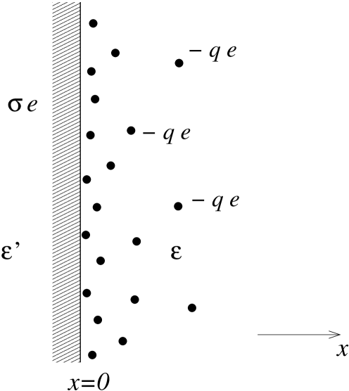
Figure 1: The general electric double layer with counter-ions only. For simplicity, we consider the homogeneous dielectric case with $\epsilon^{\prime}=\epsilon=1$ and the valence of counter-ions $q=1$.

In this paper, we restrict ourselves to a single electric double layer with counter-ions only, see the geometry in Fig. 1. The system is $\nu$-dimensional ($\nu\geq 2$), inhomogeneous along the $x$-axis and translationally invariant along all remaining $\nu-1$ spatial axes. The large macro-ion is approximated by a hard wall filled by a material of dielectric constant $\varepsilon^{\prime}$ in the half-space $x<0$. Its surface at $x=0$ is charged by a fixed uniform surface-charge density $\sigma e$, $e$ being the elementary charge and say $\sigma>0$. The wall is impenetrable to the $q$-valent counter-ions moving freely in the complementary half-space $x>0$. To simplify the notation, we set the valence $q=1$; to restore the $q$-dependence we have to substitute $\sigma\to\sigma/q$ and $e\to qe$ in final formulas. The counter-ions are classical point-like particles immersed in a solution of dielectric constant $\varepsilon$. For simplicity, we consider the homogeneous dielectric case with $\varepsilon^{\prime}=\varepsilon=1$ (vacuum in Gauss units), without electrostatic image forces. The system is in thermal equilibrium at temperature $T$, or inverse temperature $\beta=1/(k_{\rm B}T)$. Although the dimension three (3D) is of primary physical interest, many works deal with the two-dimensional (2D) version of Coulomb systems interacting logarithmically which are sometimes exactly solvable, at a specific free-fermion coupling Jancovici81 ; Jancovici84 ; Gaudin85 ; Cornu87 ; Cornu89 (for review, see Jancovici92 ) or, in the case of the Coulomb gas of point $\pm$ charges, in the whole stability interval of temperatures Samaj00 ; Samaj03 .

The model became, due to its relative simplicity, the cornerstone for developing theoretical methods to general Coulomb systems. The weak-coupling (high-temperature) limit is described by the Poisson-Boltzmann (PB) mean-field approach Andelman06 and by its systematic improvements via the loop expansion Attard88a ; Attard88b ; Podgornik90 ; Netz00 . The opposite strong-coupling (low-temperature) limit was pioneered by Rouzina and Bloomfield Rouzina96 and developed subsequently in Grosberg02 ; Levin02 ; a basic ingredient was the formation of a 2D Wigner layer of counter-ions close to the charged wall. In the field-theoretical approach of Netz and collaborators Moreira01 ; Netz01 ; Moreira02 ; Naji05 , the leading strong-coupling behavior stems from a single-particle theory and the next correction orders correspond to a virial fluid expansion in inverse powers of the coupling constant. A comparison with Monte Carlo simulations shows the adequacy of the method to capture the leading strong-coupling behavior, but its failure for the first correction. Recently Samaj11a ; Samaj11b ; Samaj11c , a strong-coupling theory starting from the 2D Wigner crystal was proposed which reproduces the leading single-particle picture of the virial method and at the same time gives the first correction which is in excellent agreement with Monte Carlo data.

For dense homogeneous and inhomogeneous Coulomb fluids in thermal equilibrium, like the jellium or the two-component Coulomb gas, there exists a variety of exact sum rules which relate the particle one-body and two-body densities, for an old review see Martin88 . The necessary conditions for these sum rules is that the Coulomb fluid exhibits good screening properties, i.e. the particle correlation functions or the averaged charge inhomogeneity, say close to a wall, exhibit a short-range (usually exponential) decay to zero. The bulk charge-charge correlation functions satisfy, in any dimension, the zeroth-moment and second-moment Stillinger-Lovett conditions Stillinger68a ; Stillinger68b . In 2D, also the compressibility Vieillefosse75 ; Baus78 and higher-moment Kalinay00 ; Jancovici00 sum rules are available explicitly. For semi-infinite domains constrained by planar wall surfaces, the density of particles at the wall is related to the bulk pressure via the contact theorem Henderson78 ; Henderson79 ; Henderson81 ; Carnie81a ; Wennerstrom82 . The Carnie and Chan generalization to inhomogeneous fluids of the second-moment Stillinger-Lovett bulk condition gives the dipole sum rule Carnie81b ; Carnie83 . A sum rule for the variation of the particle density with respect to the external electrical field was derived by Blum et al. Blum81 . The WLMB (Wertheim, Lovett, Mou, Buff) equations Lovett76 ; Wertheim76 , originally derived for neutral particles, were adapted to charged systems as well Jancovici04 . The charge-charge correlation functions decay slowly as an inverse-power law along the wall Usenko76 ; Jancovici82a and a sum rule for the amplitude function holds Jancovici82b ; Jancovici95 ; Samaj10 . A relation between this algebraic tail and the dipole moment was found in Jancovici01 .

The aim of this work is to investigate whether the known sum rules apply to our electric double layer with counter-ions only. The problem is that the present model does not exhibit good screening properties: the density profile and the amplitude function of the long-range tail along the wall exhibit a long-range (inverse-power) tail at large distances from the wall. We check the sum rules in two exactly solvable cases: the PB theory in any dimension $\nu\geq 2$ and at the special free-fermion coupling $\beta e^{2}=2$ in 2D. In both cases, all sum rules hold which indicates their extended applicability. The sum rules provide exact information about the model and represent strong constraints which have to be fulfilled within a reasonable theoretical description.

The paper is organized as follows. The known sum rules are listed in sect. 2. The PB treatment in sect. 3 implies the inhomogeneous density profile; the correlation functions are evaluated with this profile by using a method which is alternative to the one-loop level of the field theory Netz00 . The complete solution of the 2D model at the free-fermion coupling $\beta e^{2}=2$ is the subject of sect. 4. Sect. 5 is the Conclusion.

2 List of sum rules

We consider the homogeneous dielectric case $\varepsilon^{\prime}=\varepsilon=1$ of the electric double layer pictured in Fig. 1. Particles are constrained to the semi-infinite $\nu$-dimensional Euclidean domain. Each point of this domain ${\bf r}=(x,{\bf R})$ has the component $x\in[0,\infty]$, along which the system is inhomogeneous, and the remaining $\nu-1$ perpendicular (unbounded) components ${\bf R}\in[-\infty,\infty]^{\nu-1}$, along which the system is homogeneous and translationally invariant.

In dimension $\nu$, the Coulomb potential $v$ at point ${\bf r}$, induced by a unit charge at the origin ${\bf 0}$, is defined as the solution of the Poisson equation

$$\Delta v({\bf r})=-s_{\nu}\delta({\bf r}),$$ (1)

where $s_{\nu}=2\pi^{\nu/2}/\Gamma(\nu/2)$ (in particular, $s_{2}=2\pi$ and $s_{3}=4\pi$) is the surface area of the $\nu$-dimensional unit sphere. Explicitly,

$$v({\bf r})=\left\{\begin{array}[]{ll}-\ln(r/r_{0})&\mbox{if $\nu=2$,}\cr&\cr r^{2-\nu}/(\nu-2)&\mbox{otherwise,}\end{array}\right.$$ (2)

where $r=|{\bf r}|$ and $r_{0}$ is a length scale. Dimension one has special features and is excluded from the analysis. The definition of the Coulomb potential (1) implies the characteristic small-$k$ singularity $\hat{v}(k)=1/k^{2}$ in the Fourier space. This maintains many generic properties, like screening and the corresponding sum rules, of “real” 3D Coulomb systems with $1/r$ interactions. Dimensions $\nu=2,3$ are of special physical interest. The 2D logarithmic potential corresponds to the interaction of infinite uniformly charged lines which are perpendicular to the given plane. Since the point-like particles possess the same charge, no short-range regularization of the Coulomb potential is needed and the thermodynamics is well defined.

The Hamiltonian of particles $i=1,\ldots,N$ with charge $-e$ at positions $\{{\bf r}_{i}=(x_{i},{\bf R}_{i})\}$ and the fixed surface charge density $\sigma e$ at $x=0$ reads

$$H=e^{2}\sum_{i<j}v(|{\bf r}_{i}-{\bf r}_{j}|)+e^{2}\sigma\frac{s_{\nu}}{2}\sum_{i}x_{i}.$$ (3)

In the canonical ensemble with the requirement of the overall neutrality, the thermal average at the inverse temperature $\beta$ will be denoted by $\langle\cdots\rangle$. At one-particle level, we introduce the particle density

$$n({\bf r})\equiv n(x)=\left\langle\textstyle{\sum_{i}}\delta({\bf r}-{\bf r}_{i})\right\rangle.$$ (4)

At two-particle level, we have the two-body densities

$$n_{2}({\bf r},{\bf r}^{\prime}) \equiv n_{2}(x,x^{\prime};|{\bf R}-{\bf R}^{\prime}|)=n_{2}(x^{\prime},x;|{\bf R}-{\bf R}^{\prime}|)$$ (5)

$$= \left\langle\textstyle{\sum_{i\neq j}}\delta({\bf r}-{\bf r}_{i})\delta({\bf r}^{\prime}-{\bf r}_{j})\right\rangle.$$

The corresponding (truncated) Ursell functions

$$n_{2}^{(\rm T)}({\bf r},{\bf r}^{\prime})=n_{2}({\bf r},{\bf r}^{\prime})-n({\bf r})n({\bf r}^{\prime})$$ (6)

go to zero at large distances $|{\bf r}-{\bf r}^{\prime}|\to\infty$. In the above formulas, we used invariance with respect to translations along the wall surface and rotations around the $x$ axis.

Now we list all known Coulomb sum rules, adapted to our system, forgetting for a while that the necessary conditions like screening do not apply.

2.1 Sum rules involving the particle density only

The overall electroneutrality of the system is equivalent to the condition

$$\int_{0}^{\infty}{\rm d}x\,n(x)=\sigma.$$ (7)

Thus the particle density $n(x)$ must go to zero faster than $1/x$ as $x\to\infty$.

The contact theorem for planar wall surfaces Henderson78 ; Henderson79 ; Henderson81 ; Carnie81a ; Wennerstrom82 relates the contact density of particles $n(0)$ to the bulk pressure of the fluid $P$ as follows

$$\beta P=n(0)-\frac{1}{2}\beta e^{2}s_{\nu}\sigma^{2}.$$ (8)

Since the density of particles vanishes in the bulk $x\to\infty$, we have $P=0$ and the exact constraint

$$n(0)=\frac{1}{2}\beta e^{2}s_{\nu}\sigma^{2}.$$ (9)

2.2 Electroneutrality and dipole sum rules

Two sum rules for inhomogeneous Coulomb fluids have the origin directly in the zeroth-moment and second-moment Stillinger-Lovett conditions for the bulk correlation functions Stillinger68a ; Stillinger68b .

The electroneutrality condition with a particle fixed at some point takes the form

$$n(x)=-\int_{0}^{\infty}{\rm d}x^{\prime}\int{\rm d}{\bf R}\,n_{2}^{(\rm T)}(x,x^{\prime};R).$$ (10)

The dipole sum rule

$$\int_{0}^{\infty}{\rm d}x\int_{0}^{\infty}{\rm d}x^{\prime}\int{\rm d}{\bf R}\,(x^{\prime}-x)n_{2}^{(\rm T)}(x,x^{\prime};R)=-\frac{1}{s_{\nu}\beta e^{2}}$$ (11)

follows directly from the Carnie and Chan generalization to inhomogeneous fluids of the second-moment Stillinger-Lovett bulk condition Carnie81b ; Carnie83 . Note that the integrals over $x$ and $x^{\prime}$ in (11) cannot be interchanged since the integrated function is not absolutely integrable; if the interchanging of integrations would be possible, the result is zero since $(x^{\prime}-x)$ changes its sign under the exchange $x\leftrightarrow x^{\prime}$ transformation.

2.3 Sum rule of Blum et al.

Blum et al. Blum81 derived a sum rule which relates the variation of the particle density $n({\bf r})$ with respect to the external electrical field $E=s_{\nu}\sigma e$ to the dipole moment with respect to a particle fixed at ${\bf r}$. For our system, the sum rule reads explicitly as

$$\frac{\partial n(x)}{\partial\sigma}=-s_{\nu}\beta e^{2}\int_{0}^{\infty}{\rm d}x^{\prime}\int{\rm d}{\bf R}\,(x^{\prime}-x)n_{2}^{(\rm T)}(x,x^{\prime};R).$$ (12)

This relation is superior to the dipole sum rule (11) which results by integrating both sides of (12) over $x\in[0,\infty]$ and then considering the electroneutrality condition (7).

2.4 The WLMB equations for charged systems

The WLMB equations Lovett76 ; Wertheim76 were originally derived for neutral particles. Their generalization to charged systems Martin88 ; Jancovici04 relates the gradient of the density to an integral of the corresponding two-body Ursell function over the boundary:

$$\frac{\partial n(x)}{\partial x}=\int{\rm d}{\bf R}\,n_{2}^{(\rm T)}(0,x;R).$$ (13)

Note that integrating this formula over $x\in[0,\infty]$ and taking $n(x\to\infty)=0$, we recover the electroneutrality condition (10) for the special case $x=0$.

2.5 Long-range decay along the wall

Because of asymmetry of the screening cloud around a particle sitting near the wall, the two-body Ursell functions decay slowly along the wall Usenko76 ; Jancovici82a . Using linear response in combination with a simple macroscopic argument based on the electrostatic method of images Jancovici82b ; Jancovici95 ; Samaj10 , one expects an asymptotic inverse-power law behavior

$$n_{2}^{(\rm T)}(x,x^{\prime};R)\simeq\frac{f(x,x^{\prime})}{R^{\nu}},\qquad R\to\infty.$$ (14)

In the $(\nu-1)$-dimensional Fourier ${\bf k}$-space with respect to ${\bf R}$, defined by

$$\hat{g}(x,x^{\prime};k) = \int{\rm d}{\bf R}\exp(-{\rm i}{\bf k}\cdot{\bf R})g(x,x^{\prime};R),$$

$$g(x,x^{\prime};R) = \int\frac{{\rm d}{\bf k}}{(2\pi)^{\nu-1}}\exp({\rm i}{\bf k}\cdot{\bf R})\hat{g}(x,x^{\prime};k),$$ (15)

this behavior is governed by the kink at ${\bf k}={\bf 0}$ Gelfand64 of the small wave number behavior

$$\hat{n}_{2}^{(\rm T)}(x,x^{\prime};k)=\hat{n}_{2}^{(\rm T)}(x,x^{\prime};0)-\frac{s_{\nu}}{2}f(x,x^{\prime})k+\cdots.$$ (16)

The function $f(x,x^{\prime})$, which is symmetric in $x$ and $x^{\prime}$, obeys the sum rule Jancovici82b ; Jancovici95 ; Samaj10

$$\int_{0}^{\infty}{\rm d}x\int_{0}^{\infty}{\rm d}x^{\prime}\,f(x,x^{\prime})=-\frac{2}{\beta e^{2}s_{\nu}^{2}}.$$ (17)

It is interesting that for all exactly solvable cases the function $f(x,x^{\prime})$ takes the product form

$$f(x,x^{\prime})=-g(x)g(x^{\prime}).$$ (18)

The decoupling of coordinates $x$ and $x^{\prime}$ is intuitively due to the fact that the lateral distance between the points ${\bf r}$ and ${\bf r}^{\prime}$ goes to infinity and so the $x$-coordinates of the two points become mutually uncorrelated.

A relation between the algebraic tail of the correlation function along the wall and the dipole moment of that function was found in Ref. Jancovici01 :

$$\int_{0}^{\infty}{\rm d}x^{\prime}\int{\rm d}{\bf R}\,(x^{\prime}-x)n_{2}^{(\rm T)}(x,x^{\prime};R)=\frac{s_{\nu}}{2}\int_{0}^{\infty}{\rm d}x^{\prime}\,f(x,x^{\prime})$$ (19)

for any $x\geq 0$. The integration of this relation over $x\in[0,\infty]$ leads to the equality which is consistent with the previous sum rules (11) and (17).

3 Poisson-Boltzmann theory

We adapt to arbitrary $\nu\geq 2$ dimensions the derivation of the 3D PB theory by Andelman Andelman06 which was formulated originally longtime ago by Gouy Gouy10 and Chapman Chapman13 .

The density of counter-ions $n(x)$ corresponds to the charge density $\rho(x)=-en(x)$. The average electrostatic potential $\phi$ at distance $x$ from the wall satisfies the Poisson equation

$$\frac{{\rm d}^{2}\phi(x)}{{\rm d}x^{2}}=-s_{\nu}\rho(x).$$ (20)

In the mean-field approach, the particle energy at $x$ is approximated by $-e\phi(x)$ in the corresponding Boltzmann factor:

$$n(x)=n_{0}\exp\left[\beta e\phi(x)\right].$$ (21)

The boundary condition for the electric field reads

$$\frac{{\rm d}\phi(x)}{{\rm d}x}\Big{|}_{x=0}=-s_{\nu}\sigma e<0.$$ (22)

We introduce the Gouy-Chapmann length

$$b=\frac{2}{\beta e^{2}\sigma s_{\nu}}$$ (23)

and the dimensionless electric potential $\psi(x)=\beta e\phi(x)$, $n(x)=n_{0}\exp[\psi(x)]$, which satisfies the equations

$$\frac{{\rm d}^{2}\psi(x)}{{\rm d}x^{2}}=\frac{2n_{0}}{\sigma b}\exp\left[\psi(x)\right],\qquad\frac{{\rm d}\psi(x)}{{\rm d}x}\Big{|}_{x=0}=-\frac{2}{b}.$$ (24)

Their solution is

$$\psi(x)=c-2\ln(x+b),\qquad n_{0}{\rm e}^{c}=\sigma b.$$ (25)

The corresponding particle density

$$n(x)=\frac{\sigma b}{(x+b)^{2}}$$ (26)

evidently satisfies both the electroneutrality condition (7) and the contact theorem (9). Note that the spatial dimension $\nu$ enters only through the definition of the Gouy-Chapmann length (23).

The correlation functions can be evaluated with the density profile (26) by using the one-loop level of the field-theoretical method of Netz and Orland Netz00 . The correlation functions are introduced there as auxiliary quantities to deduce the first correction to the density profile. Their exact meaning is not specified. This is why we propose an alternative derivation. It follows from the general theory of Coulomb fluids, namely the Ornstein-Zernike equation

$$h({\bf r},{\bf r}^{\prime})=c({\bf r},{\bf r}^{\prime})+\int{\rm d}{\bf r}^{\prime\prime}c({\bf r},{\bf r}^{\prime\prime})n({\bf r}^{\prime\prime})h({\bf r}^{\prime\prime},{\bf r}^{\prime}),$$ (27)

which relates the truncated pair correlation

$$h({\bf r},{\bf r}^{\prime})=\frac{n_{2}^{(\rm T)}({\bf r},{\bf r}^{\prime})}{n({\bf r})n({\bf r}^{\prime})}$$ (28)

to the so-called direct correlation function $c$. For particles interacting via the Coulomb potential $v$, the leading term of $c$ reads Jancovici82a ; Kalinay00 ; Jancovici00

$$c({\bf r},{\bf r}^{\prime})\simeq-\beta e^{2}v({\bf r},{\bf r}^{\prime}).$$ (29)

Inserting this expression into (27), applying to both sides the Laplacian with respect to ${\bf r}$ and using the Poisson equation (1), we obtain

$$\left[\Delta_{\bf r}-\beta e^{2}s_{\nu}n(x)\right]h({\bf r},{\bf r}^{\prime})=\beta e^{2}s_{\nu}\delta({\bf r}-{\bf r}^{\prime}),\quad x,x^{\prime}>0$$ (30)

and

$$\Delta_{\bf r}h({\bf r},{\bf r}^{\prime})=0,\qquad x<0,x^{\prime}>0.$$ (31)

In the Fourier space with respect to ${\bf R}$ (15), we get

$$\left[\frac{{\rm d}^{2}}{{\rm d}x^{2}}-\frac{2}{(x+b)^{2}}-k^{2}\right]\hat{h}(x,x^{\prime};k)=\beta e^{2}s_{\nu}\delta(x-x^{\prime}),\phantom{aaa}$$

$$x,x^{\prime}>0\phantom{aaa}$$ (32)

and

$$\left[\frac{{\rm d}^{2}}{{\rm d}x^{2}}-k^{2}\right]\hat{h}(x,x^{\prime};k)=0,\quad x<0,x^{\prime}>0.$$ (33)

These equations are supplemented by the conditions that $\hat{h}(x,x^{\prime};k)$ and ${\rm d}\hat{h}(x,x^{\prime};k)/{\rm d}x$ are continuous at $x=0$ and by regularity $\hat{h}(x,x^{\prime};k)\to 0$ as $x\to\pm\infty$. The formal solution of Eq. (32) reads Courant53

$$\frac{\hat{h}(x,x^{\prime};k)}{\beta e^{2}s_{\nu}} = \frac{1}{W}\left[\varphi^{+}(x)\varphi^{-}(x^{\prime})\theta(x-x^{\prime})\right.$$

$$\left.+\varphi^{+}(x^{\prime})\varphi^{-}(x)\theta(x^{\prime}-x)\right]+A\varphi^{+}(x)\varphi^{+}(x),$$

where $A$ is a free parameter, $\theta$ the Heaviside step function

$$\theta(x)=\left\{\begin{array}[]{ll}1&\mbox{if $x>0$,}\cr 0&\mbox{if $x<0$,}\end{array}\right.$$ (35)

the functions $\varphi^{\pm}$ are given by

$$\left[\frac{{\rm d}^{2}}{{\rm d}x^{2}}-\frac{2}{(x+b)^{2}}-k^{2}\right]\varphi^{\pm}(x)=0,\quad\varphi^{\pm}(\pm\infty)=0$$ (36)

and the Wronskian

$$W=\varphi^{-}(x)\frac{\rm d}{{\rm d}x}\varphi^{+}(x)-\varphi^{+}(x)\frac{\rm d}{{\rm d}x}\varphi^{-}(x)$$ (37)

does not depend on $x$, as one can prove directly by differentiating $W$ with respect to $x$ and then using differential equations (36) for $\varphi^{\pm}$. The solutions of Eqs. (36) read

$$\varphi^{\pm}(x)=\left[1\pm\frac{1}{k(x+b)}\right]\exp\left[\mp k(x+b)\right]$$ (38)

and the Wronskian $W=-2k$. The formal solution of Eq. (33) is

$$\frac{\hat{h}(x,x^{\prime};k)}{\beta e^{2}s_{\nu}}=B\varphi^{+}(x^{\prime})\exp(kx),$$ (39)

where $B$ is a free parameter. The continuity conditions at $x=0$ determine the parameters $A$ and $B$ as follows

$$A = -\frac{1}{2k}{\rm e}^{2kb}\frac{1}{1+2(kb)+2(kb)^{2}},$$

$$B = -\frac{1}{k}{\rm e}^{kb}\frac{(kb)^{2}}{1+2(kb)+2(kb)^{2}}.$$ (40)

After some algebra, the small-$k$ expansion of the truncated pair correlation is found to be

$$\frac{\hat{h}(x,x^{\prime};k)}{\beta e^{2}s_{\nu}} = -\frac{1}{3}\frac{x_{<}^{3}+3bx_{<}^{2}+3b^{2}x_{<}+3b^{3}}{(x+b)(x^{\prime}+b)}$$ (41)

$$+\frac{b^{4}}{(x+b)(x^{\prime}+b)}k+\cdots,$$

where $x_{<}=\min(x,x^{\prime})$.

The partial Fourier transform of the two-body density $\hat{n}_{2}^{(\rm T)}(x,x^{\prime};k)=n(x)n(x^{\prime})\hat{h}(x,x^{\prime};k)$ has the small-$k$ expansion

$$\hat{n}_{2}^{(\rm T)}(x,x^{\prime};k) = -\frac{4}{3\beta e^{2}s_{\nu}}\frac{x_{<}^{3}+3bx_{<}^{2}+3b^{2}x_{<}+3b^{3}}{(x+b)^{3}(x^{\prime}+b)^{3}}$$ (42)

$$+\frac{4}{\beta e^{2}s_{\nu}}\frac{b^{4}}{(x+b)^{3}(x^{\prime}+b)^{3}}k+\cdots.$$

The first term of this expansion determines the integral

$$\int{\rm d}{\bf R}\,n_{2}^{(\rm T)}(x,x^{\prime};R)$$

$$\qquad=-\frac{4}{3\beta e^{2}s_{\nu}}\frac{x_{<}^{3}+3bx_{<}^{2}+3b^{2}x_{<}+3b^{3}}{(x+b)^{3}(x^{\prime}+b)^{3}}.$$ (43)

The presence of the second term in (42) signalizes the asymptotic behavior of type (14). With regard to formula (16), the function $f(x,x^{\prime})$ has the long-range form

$$f(x,x^{\prime})=-\frac{8}{\beta e^{2}s_{\nu}^{2}}\frac{b^{4}}{(x+b)^{3}(x^{\prime}+b)^{3}}.$$ (44)

Notice that the product form (18) takes place with $g(x)=b^{2}\sqrt{8/(\beta e^{2}s_{\nu}^{2})}/(x+b)^{3}$. Using the last two relations it is easy to show that the sum rules (10), (11), (12), (13), (17) and (19) hold, in spite of the long-range nature of the density profile $n(x)$ and the function $f(x,x^{\prime})$.

4 2D model at the free-fermion coupling

The 2D version of the present model is mappable onto free fermions at the special coupling $\Gamma\equiv\beta e^{2}=2$ Jancovici84 ; Samaj11c . Here, we consider the Grassmann formulation of the Coulomb system on the surface of a semi-infinite cylinder of circumference $W$, i.e. the strip with $x\in[0,\infty]$ and periodic boundary conditions along $y\in[0,W]$ Samaj11c . The charge line density $\sigma e$ at $x=0$ is neutralized by $N=\sigma W$ particles of charge $-e$. At the coupling $\Gamma=2$, the renormalized one-body potential acting on particles reads

$$w_{\rm ren}(x)=\frac{4\pi}{W^{2}}\exp\left(-\frac{2\pi}{W}x\right).$$ (45)

In terms of two sets of anticommuting Grassmann variables $\xi_{j}$ and $\psi_{j}$, defined on a discrete chain of $N$ sites $j=0,1,\ldots,N-1$, the partition function of the system is expressible as

$$Z_{N}=\int{\cal D}\psi{\cal D}\xi\,{\rm e}^{S(\xi,\psi)},\qquad S(\xi,\psi)=\sum_{j=0}^{N-1}\xi_{j}w_{j}\psi_{j},$$ (46)

where the diagonal interaction matrix has the elements

$$w_{j}=W\int_{0}^{\infty}{\rm d}x\,w_{\rm ren}(x)\exp\left(-\frac{4\pi}{W}jx\right)=\frac{1}{j+\frac{1}{2}}.$$ (47)

Due to the diagonalized form of the anticommuting action $S(\xi,\psi)$, the partition function is available explicitly as the product of diagonal matrix elements

$$Z_{N}=w_{0}w_{1}\cdots w_{N-1}.$$ (48)

Within the Grassmann formalism, the particle density is given by

$$n(x)=w_{\rm ren}(x)\sum_{j=0}^{N-1}\langle\xi_{j}\psi_{j}\rangle\exp\left(-\frac{4\pi}{W}jx\right),$$ (49)

where the two-correlator

$$\langle\xi_{j}\psi_{j}\rangle\equiv\frac{1}{Z_{N}}\int{\cal D}\psi{\cal D}\xi\,{\rm e}^{S(\xi,\psi)}\xi_{j}\psi_{j}=\frac{\partial}{\partial w_{j}}\ln Z_{N}=\frac{1}{w_{j}}.$$ (50)

In the thermodynamic limit $N\to\infty$, which is equivalent to $W\to\infty$ keeping the ratio $N/W=\sigma$ fixed, we pass from the semi-infinite cylinder to a 2D half-space. The variable $t=(j+\frac{1}{2})/(N-\frac{1}{2})$ becomes continuous and Eqs. (49), (50) imply the density profile

$$n(x) = 4\pi\sigma^{2}\int_{0}^{1}{\rm d}t\,t\exp(-4\pi\sigma tx)$$ (51)

$$= 4\pi\int_{0}^{\sigma}{\rm d}s\,s\exp(-4\pi sx)$$

$$= \frac{1}{4\pi x^{2}}\left[1-\left(1+4\pi\sigma x\right){\rm e}^{-4\pi\sigma x}\right].$$

Like in the PB approach, the density has a long-range tail: $n(x)\simeq 1/(4\pi x^{2})$ as $x\to\infty$. It is easy to verify that that the electroneutrality condition (7) and the contact theorem (9), taken with $\beta e^{2}=2$ and $s_{2}=2\pi$, hold.

The two-body densities are given by

$$n_{2}({\bf r},{\bf r}^{\prime}) = w_{\rm ren}(x)w_{\rm ren}(x^{\prime})\sum_{j,k,j^{\prime},k^{\prime}=0\atop(j+j^{\prime}=k+k^{\prime})}^{N-1}\langle\xi_{j}\psi_{k}\xi_{j^{\prime}}\psi_{k^{\prime}}\rangle$$ (52)

$$\times\exp\left(-\frac{2\pi}{W}[jz+k\bar{z}+j^{\prime}z^{\prime}+k^{\prime}\bar{z}^{\prime}]\right),$$

where $z=x+{\rm i}y$ and $\bar{z}=x-{\rm i}y$ are the complex coordinates of the point ${\bf r}=(x,y)$. Due to the diagonal form of the action $S(\xi,\psi)$, the four-correlator $\langle\xi_{j}\psi_{k}\xi_{j^{\prime}}\psi_{k^{\prime}}\rangle$ can be calculated using the Wick theorem, with the result

$$\langle\xi_{j}\psi_{k}\xi_{j^{\prime}}\psi_{k^{\prime}}\rangle=\frac{1}{w_{j}w_{j^{\prime}}}\left(\delta_{jk}\delta_{j^{\prime}k^{\prime}}-\delta_{jk^{\prime}}\delta_{j^{\prime}k}\right).$$ (53)

The first product of Kronecker functions $\delta_{jk}\delta_{j^{\prime}k^{\prime}}$ leads in (52) to the term $n(x)n(x^{\prime})$ which has to be subtracted from $n_{2}({\bf r},{\bf r}^{\prime})$ to obtain the truncated Ursell function. The second product $\delta_{jk^{\prime}}\delta_{j^{\prime}k}$ produces the Ursell function of the form

$$n_{2}^{(\rm T)}(x,x^{\prime};R)=-n\left(\frac{x+x^{\prime}+{\rm i}R}{2}\right)n\left(\frac{x+x^{\prime}-{\rm i}R}{2}\right),$$ (54)

valid universaly for the finite-$W$ cylinder as well as for $W\to\infty$ 2D half-space. The integral representation of this formula for 2D half-space

$$n_{2}^{(\rm T)}(x,x^{\prime};R) = -(4\pi)^{2}\int_{0}^{\sigma}{\rm d}t\,t{\rm e}^{-2\pi t(x+x^{\prime})}\int_{0}^{\sigma}{\rm d}s\,s$$ (55)

$$\times{\rm e}^{-2\pi s(x+x^{\prime})}{\rm e}^{-2\pi{\rm i}R(t-s)}$$

is useful to derive the important integral

$$\int_{-\infty}^{\infty}{\rm d}R\,n_{2}^{(\rm T)}(x,x^{\prime};R)=-(4\pi)^{2}\int_{0}^{\sigma}{\rm d}t\,t^{2}{\rm e}^{-4\pi t(x+x^{\prime})}.$$ (56)

Using this formula, the sum rules (10), (11), (12) and (13) follow immediately. The explicit representation of the relation (54) for 2D half-space

$$n_{2}^{(\rm T)}(x,x^{\prime};R) = -\frac{1}{\pi^{2}[(x+x^{\prime})^{2}+R^{2}]^{2}}$$ (57)

$$\times\Big{\{}1-2\left[(1+2\pi\sigma(x+x^{\prime}))\cos(2\pi\sigma R)\right.$$

$$\left.+2\pi\sigma R\sin(2\pi\sigma R)\right]\exp[-2\pi\sigma(x+x^{\prime})]$$

$$+\left[(1+2\pi\sigma(x+x^{\prime}))^{2}+(2\pi\sigma R)^{2}\right]$$

$$\times\exp[-4\pi\sigma(x+x^{\prime})]\Big{\}}$$

is convenient to specify the asymptotic $R\to\infty$ tail. We obtain the expected $\nu=2$ behavior (14) with the function

$$f(x,x^{\prime})=-4\sigma^{2}\exp[-4\pi\sigma(x+x^{\prime})]$$ (58)

which is again of the product form (18) with $g(x)=2\sigma\exp(-4\pi\sigma x)$. In contrast to the PB result (44), this function is short-ranged with the exponential decay governed by the surface charge density. The sum rules (17) and (19) are fulfilled.

5 Conclusion

The model of our present interest was the electric double layer with counter-ions only. Such system is “sparse” in the sense that the particle density and two-body densities vanish at asymptotically large distances from the wall. Moreover, the large-distance decay is usually not fast enough as required by the linear response argument in the derivation of standard sum rules for classical inhomogeneous Coulomb fluids.

We studied two exactly solvable cases of the model. In the Poisson-Boltzmann limit, the long-range behavior takes place regardless of the dimension $\nu\geq 2$, for both the density profile (26) and the asymptotic amplitude function (44). As concerns the 2D version of the model at the free-fermion coupling $\Gamma=2$, the density profile (51) has the long-range tail while the asymptotic function (58) is short-ranged.

The fact that the known sum rules are reproduced in two exactly solvable cases of the electric double layer indicates their extended applicability. The dipole sum rule (11) deserves a special attention: the tendency of the system to its bulk regime with the second-moment Stillinger-Lovett condition was crucial in its derivation. As was mentioned before, the bulk regime of our model is “emptiness”.

The asymptotic amplitude functions (44) and (58) decouple themselves in $x$ and $x^{\prime}$ coordinates, in analogy with the jellium and Coulomb-gas models Jancovici04 ; Jancovici82b .

We omitted from discussion “dense” systems like the one-component plasma with a neutralizing background (jellium) or the two-component Coulomb gas of $\pm$ charges. These systems exhibit exponential screening and so the sum rules automatically hold; their verification in special cases was given e.g. in Jancovici92 ; Jancovici04 ; Jancovici82b .

The extended validity of general sum rules for inhomogeneous Coulomb fluids can serve as a useful check for the adequacy of weak-coupling physical theories. The strong-coupling theories like Samaj11a ; Samaj11b ; Samaj11c are based on the Wigner ground-state lattice structure formed by counter-ions. The Coulomb system is not in its fluid phase in that regime and the sum rules do not longer apply.

- (1) P. Attard, Adv. Chem. Phys. XCII, 1 (1996).
- (2) J.P. Hansen, H. Löwen, Annu. Rev. Phys. Chem. 51, 209 (2000).
- (3) H. Boroudjerdi, Y.-W. Kim, A. Naji, R.R. Netz, X. Schlagberger, A. Serr, Phys. Rep. 416, 129 (2005).
- (4) R. Messina, J. Phys.: Condens. Matter 21, 113102 (2009).
- (5) L. Guldbrand, B. Jönson, H. Wennerström, P. Linse, J. Chem. Phys. 80, 2221 (1984).
- (6) R. Kjellander, S. Marčelja, Chem. Phys. Lett. 112, 49 (1984).
- (7) R.J. Hunter, Foundations of Colloid Science, 2nd edition (Oxford University Press, New York, 2001).
- (8) B. Jancovici, Phys. Rev. Lett. 46, 386 (1981).
- (9) B. Jancovici, J. Stat. Phys. 34, 803 (1984).
- (10) M. Gaudin, J. Phys. (Paris) 46, 1027 (1985).
- (11) F. Cornu, B. Jancovici, J. Stat. Phys. 49, 33 (1987).
- (12) F. Cornu, B. Jancovici, J. Chem. Phys. 90, 2444 (1989).
- (13) B. Jancovici, in Inhomogeneous Fluids, edited by D. Henderson (Dekker, New York, 1992), pp. 201-237.
- (14) L. Šamaj, I. Travěnec, J. Stat. Phys. 101, 713 (2000).
- (15) L. Šamaj, J. Phys. A: Math. Gen. 36, 5913 (2003).
- (16) D. Andelman, in Soft Condensed Matter Physics in Molecular and Cell Biology, edited by W.C.K. Poon, D. Andelman (Taylor & Francis, New York, 2006), Chapt. 6.
- (17) P. Attard, D.J. Mitchell, B.W. Ninham, J. Chem. Phys. 88, 4987 (1988).
- (18) P. Attard, D.J. Mitchell, B.W. Ninham, J. Chem. Phys. 89, 4358 (1988).
- (19) R. Podgornik, J. Phys. A 23, 275 (1990).
- (20) R.R. Netz, H. Orland, Eur. Phys. J. E 1, 203 (2000).
- (21) I. Rouzina, V.A. Bloomfield, J. Phys. Chem. 100, 9977 (1996).
- (22) A.Y. Grosberg, T.T. Nguyen, B.I. Shklovskii, Rev. Mod. Phys. 74, 329 (2002).
- (23) Y. Levin, Rep. Prog. Phys. 65, 1577 (2002).
- (24) A.G. Moreira, R.R. Netz, Phys. Rev. Lett. 87, 078301 (2001).
- (25) R.R. Netz, Eur. Phys. J. E 5, 557 (2001).
- (26) A.G. Moreira, R.R. Netz, Eur. Phys. J. E 8, 33 (2002).
- (27) A. Naji, S. Jungblut, A.G. Moreira, R.R. Netz, Physica (Amsterdam) 352A, 131 (2005).
- (28) L. Šamaj, E. Trizac, Phys. Rev. Lett. 106, 078301 (2011).
- (29) L. Šamaj, E. Trizac, Phys. Rev. E 84, 041401 (2011).
- (30) L. Šamaj, E. Trizac, Eur. Phys. J. E 34, 20 (2011).
- (31) Ph.A. Martin, Rev. Mod. Phys. 60, 1075 (1988).
- (32) F.H. Stillinger, R. Lovett, J. Chem. Phys. 48, 3858 (1968).
- (33) F.H. Stillinger, R. Lovett, J. Chem. Phys. 49, 1991 (1968).
- (34) P. Vieillefosse, J.P. Hansen, Phys. Rev. A 12, 1106 (1975).
- (35) M. Baus, J. Phys. A: Math. Gen. 11, 2451 (1978).
- (36) P. Kalinay, P. Markoš, L. Šamaj, I. Travěnec, J. Stat. Phys. 98, 639 (2000).
- (37) B. Jancovici, P. Kalinay, L. Šamaj, Physica A 279, 260 (2000).
- (38) D. Henderson, L. Blum, J. Chem. Phys. 69, 5441 (1978).
- (39) D. Henderson, L. Blum, J.L. Lebowitz, J. Electroanal. Chem. 102, 315 (1979).
- (40) D. Henderson, L. Blum, J. Chem. Phys. 75, 2025 (1981).
- (41) S.L. Carnie, D.Y.C. Chan, J. Chem. Phys. 74, 1293 (1981).
- (42) H. Wennerström, B. Jönson, P. Linse, J. Chem. Phys. 76, 4655 (1982).
- (43) S.L. Carnie, D.Y.C. Chan, Chem. Phys. Lett. 77, 437 (1981).
- (44) S.L. Carnie, D.Y.C. Chan, J. Chem. Phys. 78, 2742 (1983).
- (45) L. Blum, D. Henderson, J.L. Lebowitz, Ch. Gruber, Ph.A. Martin, J. Chem. Phys. 75, 5974 (1981).
- (46) R. Lovett, C.Y. Mou, F.P. Buff, J. Chem. Phys. 65, 570 (1976).
- (47) M.S. Wertheim, J. Chem. Phys. 65, 2377 (1976).
- (48) B. Jancovici, L. Šamaj, J. Stat. Phys. 114, 1211 (2004).
- (49) A.S. Usenko, I.P. Yakimenko, Sov. Tech. Phys. Lett. 5, 549 (1976).
- (50) B. Jancovici, J. Stat. Phys. 28, 43 (1982).
- (51) B. Jancovici, J. Stat. Phys. 29, 263 (1982).
- (52) B. Jancovici, J. Stat. Phys. 80, 445 (1995).
- (53) L. Šamaj, B. Jancovici, J. Stat. Phys. 139, 432 (2010).
- (54) B. Jancovici, L. Šamaj, J. Stat. Phys. 105, 193 (2001).
- (55) I.M. Gelfand, G.E. Shilov, Generalized Functions, (Academic Press, New York, 1964).
- (56) G. Gouy, J. Phys. (Paris) 9, 457 (1910).
- (57) D.L. Chapman, Philos. Mag. 25, 475 (1913).
- (58) R. Courant, D. Hilbert, Methods of Mathematical Physics, (Interscience, New York, 1953), p. 355.