Critical scaling in random-field systems: 2 or 3 independent exponents?

Abstract

We show that the critical scaling behavior of random-field systems with short-range interactions and disorder correlations cannot be described in general by only two independent exponents, contrary to previous claims. This conclusion is based on a theoretical description of the whole $(d,N)$ domain of the $d$-dimensional random-field $O(N)$ model and points to the role of rare events that are overlooked by the proposed derivations of two-exponent scaling. Quite strikingly, however, the numerical estimates of the critical exponents of the random field Ising model are extremely close to the predictions of the two-exponent scaling, so that the issue cannot be decided on the basis of numerical simulations.

I Introduction

The critical behavior of models in the presence of a quenched random field has attracted a lot of attention over the past decades. imry-ma75 ; nattermann98 Beyond the experimental interest, such models provide a rich playground to investigate the influence of quenched disorder on the long-distance properties of a system. Their equilibrium critical point, separating a disordered, paramagnetic phase from an ordered, ferromagnetic one, is known to be controlled by a zero-temperature fixed point, with temperature being an irrelevant variable in the renormalization-group sense. Among the new features brought by such a fixed point is the violation of the “hyperscaling relation” between critical exponents. The space dimension $d$ that appears in this relation must be corrected by the exponent $\theta$ describing the flow of the renormalized temperature to zero, thereby leading to an apparent dimensional reduction from $d$ to $d-\theta$.nattermann98 ; villain85 ; fisher86

Whereas phenomenological theories take $\theta$ as an independent exponent,villain85 ; fisher86 which implies that equilibrium scaling behavior is described by three independent exponents in place of the usual two-exponent scaling for finite-temperature fixed points, two different approaches have claimed that $\theta$ is actually fixed. One is the dimensional-reduction prediction, based either on perturbation theoryaharony76 ; grinstein76 ; young77 or on the Parisi-Sourlas supersymmetric formulation.parisi79 It states that $\theta=2$ and that the exponents of the random-field model are those of the corresponding pure model in two dimension less. This prediction has been rigorously proven to be wrong in low enough dimension,Imbrie (1984); Bricmont and Kupianen (1987) and we have recently provided a complete theoretical explanation of dimensional reduction and its breakdown through a nonperturbative functional renormalization group.tarjus04 ; tissier06 ; tissier11 ; tarjus13

Another line of argument has been put forward by Schwartz and coworkers.schwartz85 ; schwartz86 The claim is that $\theta=2-\eta$, with $\eta$ the anomalous dimension of the (order parameter) field, so that scaling is described by only two independent exponents, e.g., $\eta$ and the correlation length exponent $\nu$. The derivation involves general manipulations and the result is supposed to hold for the Ising as well as the continuous version with $O(N)$ symmetry. It is also supported by heuristic considerations.schwartz86 ; binder

The problem with the above derivations is that they rely on formal manipulations that are blind to the presence of rare events or rare regions, such as avalanches or droplets, or that overlook the presence of multiple metastable states. This is known to be the reason for the failure of the simple supersymmetric formulation.Parisi (1984); tissier11 ; tarjus13 This also casts some doubt on the general validity of the order-of-magnitude estimates of the relative strength of the fluctuations carried out in Schwartz’s arguments.schwartz85 ; schwartz86

How to conclude on the validity of the two-exponent scenario proposed by Schwartz and coworkers? The question is actually quite subtle as the description is exact at the lower and the higher critical dimensions of the random-field models and it appears to be numerically very well verified in computer simulations (including a recent extensive onefytas13 ), high-temperature expansions or approximate renormalization-group treatments, mostly in $d=3$. Our contention is that it is impossible to answer the question on a pure numerical ground as the error bars will always blur the conclusion. On the contrary, with the help of the functional renormalization group (FRG), the problem can be studied for continuous values of the dimension $d$ and of the number of components $N$ of the order-parameter field. We can then show with no ambiguity that the two-exponent scenario cannot be right in general, which then reduces the corresponding prediction for the random-field Ising model in $d=3$ to a very, or even extremely,fytas13 good but by no means exact, result. We have already made this point in earlier worktissier06 ; tissier11 but in this paper, we sharpen the arguments and present extended calculations.

The rest of the paper is organized as follows. In section II, we present the the random field $O(N)$ model [RF$O(N)$M] and the scaling behavior around its critical point and in section III we summarize and discuss the predictions of the two-exponent scaling scenario. In section IV, we recall the results of the FRG for the RF$O(N)$M with $N>1$ (continuous symmetry) near the lower critical dimension for ferromagnetism, in $d=4+\epsilon$. We show that at order $\epsilon$ and $\epsilon^{2}$, the relation proposed by Schwartz and coworkers is unambiguously violated. In the next section, we consider the random field Ising model (RFIM) via a nonperturbative version of the FRG that we have previously developed. Here too, we show that the two-exponent scenario cannot be right for all dimensions between $2$ and $6$. We focus in particular on the dimensions around the critical dimension $d_{DR}\simeq 5.1$ that marks the lower limit of existence of the supersymmetric fixed point associated with the $d\rightarrow d-2$ dimensional reduction. Finally, we give some concluding remarks in section V.

II The critical behavior of random field systems

The long-distance behavior of the random field $O(N)$ model is described by the following Hamiltonian or bare action,

$$S[\bm{\varphi},\mathbf{h}]=\int_{x}\bigg{\{}\frac{1}{2}|\partial\bm{\varphi}(x)|^{2}+U_{B}(|\bm{\varphi}(x)|^{2})-\mathbf{h}(x)\bm{.}\bm{\varphi}(x)\bigg{\}},$$ (1)

where $\int_{x}\equiv\int d^{d}x$, $\bm{\varphi}(x)$ is an $N$ component field, $U_{B}(|\bm{\varphi}|^{2})=(\tau/2)|\bm{\varphi}|^{2}+(u/4!)(|\bm{\varphi}|^{2})^{2}$, and $\mathbf{h}(x)$ is a random source (a random magnetic field in the language of magnetic systems) with zero mean and a variance

$$\overline{h^{\mu}(x)h^{\nu}(y)}=\Delta_{B}\ \delta_{\mu\nu}\delta^{(d)}(x-y)$$ (2)

where $\mu,\nu=1,\cdots,N$ and an overline denotes an average over the random field. An ultra-violet (UV) momentum cutoff $\Lambda$, associated with an inverse microscopic length scale such as a lattice spacing, is also implicitly considered. We focus here on the short-range version defined above. We shall briefly comment on the long-range version in the conclusion.

Due to the presence of the random field, one needs to consider two different types of pair correlation functions of the $\bm{\varphi}$ field: the so-called connected one, $G_{con}^{\mu\nu}(x-y)=\overline{\langle\varphi^{\mu}(x)\varphi^{\nu}(y)\rangle-\langle\varphi^{\mu}(x)\rangle\langle\varphi^{\nu}(y)\rangle}$ and the disconnected one, $G_{dis}^{\mu\nu}(x-y)=\overline{\langle\varphi^{\mu}(x)\rangle\langle\varphi^{\nu}(y)\rangle}-\overline{\langle\varphi^{\mu}(x)\rangle}\;\overline{\langle\varphi^{\nu}(y)\rangle}$. At the critical point $T_{c}$, the two correlation functions behave as

$$G_{con}^{\mu\nu}(x-y)\sim\frac{T\,\delta_{\mu\nu}}{|x-y|^{d-2+\eta}}\;,$$ (3)

$$G_{dis}^{\mu\nu}(x-y)\sim\frac{\delta_{\mu\nu}}{|x-y|^{d-4+\bar{\eta}}}\;,$$

where $\eta$ is the usual anomalous dimension of the field and $\bar{\eta}$ is a priori a new exponent. Accordingly, one can also define two types of susceptibilities that diverge as one approaches the critical point from above as

$$\chi_{con}=\int_{x}G_{con}(x)\sim\left(T-T_{c}\right)^{-\gamma}\;,$$ (4)

$$\chi_{dis}=\int_{x}G_{dis}(x)\sim\left(T-T_{c}\right)^{-\bar{\gamma}}\;,$$

the former one being the usual magnetic susceptibility. [The component indices have been dropped as the functions are then proportional to $\delta_{\mu\nu}$ as in Eq. (LABEL:eq_con_disc_critical).] The exponents $\gamma$ and $\bar{\gamma}$ are related to $\eta$ and $\bar{\eta}$ via $\gamma=(2-\eta)\nu$ and $\bar{\gamma}=(4-\bar{\eta})\nu$, with $\nu$ the correlation length exponent.

The renormalized temperature is irrelevant at the fixed point controlling the critical behaviorvillain85 ; fisher86 and it flows to zero with an exponent $\theta$. As a result, the hyperscaling relation has an unusual form,

$$2-\alpha=(d-\theta)\nu\;,$$ (5)

where $\alpha$ is the specific-heat exponent. The exponents $\theta$, $\eta$, and $\bar{\eta}$ are related through

$$\theta=2+\eta-\bar{\eta}\;,$$ (6)

so that the scaling around the critical point is a priori described by three independent exponents, e.g., $\eta$, $\nu$, and $\theta$ or $\bar{\eta}$.

III The two-exponent scaling description

The $d\rightarrow d-2$ dimensional reduction predicts that $\theta=2$, i.e. $\bar{\eta}=\eta$, and furthermore that all the critical exponents are given by those of the pure model in $(d-2)$. On the other hand, the two-exponent scenario put forward by Schwartz and coworkersschwartz85 ; schwartz86 states that the exponents obey the following relations:

$$\theta=2-\eta\,,\;\;\;\bar{\eta}=2\eta\,.$$ (7)

The derivation actually also implies that the disconnected and connected correlation functions in Fourier space are related through

$$G_{dis}(q)=\frac{\Delta_{B}}{T^{2}}\,G_{con}(q)^{2}$$ (8)

at criticality and when $q\rightarrow 0$. Eq. (8) implies that the second cumulant of the random field is not renormalized and stays fixed to its bare value $\Delta_{B}$.

A stronger claim was initially made by Schwartz,schwartz85 who suggested that all the exponents of a random-field system in dimension $d$ are the same as those of its pure counterpart in a reduced dimension $d-2+\eta(d)$. This prediction was however soon shown by Bray and Moorebray85 to be already wrong for the exponent $\nu$ in the RFIM near its lower critical dimension 2 at first order in $\epsilon=d-2$. To the best of our knowledge, it was subsequently abandoned.

It is also worth mentioning that various heuristic arguments have been used to derive the above two-exponent scaling.schwartz86 ; binder For instance, one such argument states that the magnetization per spin in a finite-size system of linear size $L$ (we consider here the RFIM for simplicity), which scales as $L^{-(d-4+\bar{\eta})/2}$, is given for a typical realization of the random field by the average magnetic susceptibility $\chi_{con,L}\sim L^{2-\eta}$ times the mean random field $\overline{h}_{L}$ which scales as $L^{-d/2}$:

$$m_{L}\sim L^{-(d-4+\bar{\eta})/2}\sim\chi_{con,L}\,\overline{h}_{L}\sim L^{2-\eta}L^{-d/2}\,.$$ (9)

It immediately results that $\bar{\eta}=2\eta$.

In the case of the RFIM, the two-exponent scenario is exact at and near the lower critical dimension in first order in $\epsilon=d-2$, as shown in Ref. [bray85, ], and it is also somewhat trivially expected at the upper dimension $d=6$ and in first order in $\epsilon=6-d$ as both $\eta$ and $\bar{\eta}$ are zero and the mean-field result $\theta=2$ still applies. In between, numerical studies via high-temperature expansions in $d=3,4,5$gofman93 and computer simulations in $d=3$, confirm that $\bar{\gamma}$ is very close to $2\gamma$, and $\bar{\eta}$ to $2\eta$, certainly within the accuracy of the methods.

However, as mentioned in the Introduction, a fundamental problem remains that the proposed derivations of the two-exponent scaling involve, beyond formal manipulations, estimates of the relative order of magnitude of the fluctuations that essentially rely on factorization approximations and the central-limit theorem in the limit of large system size (see e.g. the above heuristic argument). All of the derivations are therefore blind to rare events, rare regions or rare samples, which, precisely, have been shown to be crucial in disordered systems near zero-temperature fixed points.villain85 ; fisher86 ; droplet_bray ; droplet_fisher ; fisherFRG ; balents96 ; FRGledoussal-chauve ; BLbalents05 ; FRGledoussal-wiese ; static-distrib_ledoussal ; BLledoussal10 ; tissier06 ; tissier11 ; tarjus13 .

In the absence of rigorous derivations, numerical evidence, no matter how good, is insufficient to establish the validity of the scenario, because of unavoidable uncertainty. Quite the contrary, we show below that the two-exponent description, which is claimed to apply to random-field systems below their upper critical dimension irrespective of the number of components $N$ and of the dimension $d$, cannot be valid in general and, as a consequence, has no rigorous foundations at this point.

IV The RFO(N)M near $d=4$

Near the lower critical dimension for ferromagnetism, which is equal to $d=4$ in this case, the long-distance physics of the RF$O(N)$M is captured by a nonlinear $\sigma$ model that in turn can be studied through a perturbative but functional RG.fisher85 The resulting FRG flow equations in $d=4+\epsilon$ have been studied at one-fisher85 ; feldman01 ; tissier06 and two-tissier06b ; ledoussal06 loop order.

The dimensionless second cumulant of the renormalized random field is a function $\Delta(z)$ (where $z$ is the cosine of the angle between fields in two different copies of the systemfisher85 ; tissier06 ) and it obeys the following RG equation at one loop:

$$k\partial_{k}\Delta_{k}(z)=\epsilon\Delta_{k}(z)-\bigg{[}z\Delta_{k}(z)^{2}+(N-3)\Delta_{k}(1)\Delta_{k}(z)$$ (10)

$$+(N-3+4z^{2})\Delta_{k}(z)\Delta_{k}^{\prime}(z)-(N+1)z\Delta_{k}(1)\Delta_{k}^{\prime}(z)$$

$$-z(1-z^{2})\Delta_{k}(z)\Delta_{k}^{\prime\prime}(z)+(1-z^{2})\Delta_{k}(1)\Delta_{k}^{\prime\prime}(z)$$

$$-3z(1-z^{2})\Delta_{k}^{\prime}(z)^{2}+(1-z^{2})^{2}\Delta_{k}^{\prime}(z)\Delta_{k}^{\prime\prime}(z)\bigg{]}\,,$$

where $k$ is the running infrared (IR) momentum cutoff, a prime denotes a derivative, and $\Delta_{k}(z)$ [which, up to a multiplicative constant, was denoted $R^{\prime}(z)$ in previous publications] is of order $\epsilon$ near the fixed point. One can moreover define two running exponents $\eta_{k}$ and $\bar{\eta}_{k}$ as follows:

$$\eta_{k}=\Delta_{k}(1),\;\bar{\eta}_{k}=-\epsilon+(N-1)\Delta_{k}(1)\,.$$ (11)

They converge to the fixed point values $\eta$, $\bar{\eta}$ when $k\rightarrow 0$. The corresponding equations at two-loop order are given in Ref. [tissier06b, ] and are not reproduced here.

A numerical and analytical investigation of these FRG equationstissier06 ; tissier06b ; baczyk13b shows that above a critical value of the number of components, $N_{DR}=18-\frac{49}{5}\epsilon$, there exists a fixed point that corresponds to the $d\rightarrow d-2$ dimensional reduction, with $\bar{\eta}=\eta=\frac{\epsilon}{N-2}-\frac{(N-1)\epsilon^{2}}{(N-2)^{2}}$. Above a slightly higher value, $N_{cusp}=2(4+3\sqrt{3})-3(2+3\sqrt{3})\epsilon/2$,baczyk13b this fixed point is stable and describes the critical behavior of the RF$O(N)$M (see also Ref. [sakamoto06, ]). In this domain of $N$, critical scaling is therefore described by $\bar{\eta}=\eta$ and $\theta=2$, which contradicts the predictions of Schwartz and coworkers.schwartz85 ; schwartz86

Below $N_{cusp}$, the stable fixed point is now characterized by a nonanalyticity in the functional dependence of the renormalized disorder cumulant [$\Delta_{*}(z)-\Delta_{*}(1)\sim\sqrt{1-z}$ when $z\rightarrow 1$] that is strong enough to break the dimensional-reduction prediction, with therefore $\bar{\eta}>\eta$. However, the possibility that this nonanalytic “cuspy” fixed point is characterized by the equality $\bar{\eta}=2\eta$ is invalidated by the results. We display the ratio $(2\eta-\bar{\eta})/\eta$ as a function of $N$ at one-loop order in Fig. 1. (The results are confirmed at two-loop order.) The ratio is equal to 1 above $N_{cusp}\simeq 18.3923$ and decreases continuously as $N$ decreases. At the endpoint value at which $\Delta_{*}(1)$ diverges, $N_{c}=2.8347\cdots$, it reaches a strictly positive value of $3-N_{c}\simeq 0.1653\cdots$. We stress that the output can be obtained with an arbitrary precision, which is quite different from simulations.

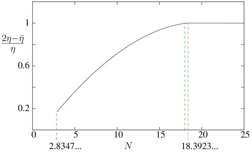
Figure 1: Ratio $(2\eta-\bar{\eta})/\eta$ as a function of $N$ for the RF$O(N)$M in $d=4+\epsilon$ at one-loop order. Above $N_{cusp}=2(4+3\sqrt{3})\simeq 18.3923\cdots$ the stable fixed point is associated with the $d\rightarrow d-2$ dimensional reduction and $(2\eta-\bar{\eta})/\eta=1$. Below $N_{DR}=18$ (marked by the leftmost vertical dashed line), the critical behavior is described by a “cuspy” fixed point and dimensional reduction breaks down but $(2\eta-\bar{\eta})/\eta$ is generically $>0$. In a small interval $N_{DR}<N<N_{cusp}$ the two fixed points coexist, but the dimensional-reduction one is unstable to a nonanalytic, “cuspy” perturbation.

V The RFIM near $d_{DR}\simeq 5.1$

The main result proving that the two-exponent scaling is generically inexact in the short-range RFIM is that there exists a range of dimension below the upper critical one, $d=6$, for which the $d\rightarrow d-2$ dimensional reduction is valid and therefore for which $\bar{\eta}=\eta\neq 2\eta$ and $\theta=2\neq 2-\eta$. The arguments establishing this result are as follows:

(i) The fixed point associated with dimensional reduction proceeds continuously from the Gaussian fixed point in $d=6$ as one lowers $d$. It is characterized by the absence of a linear cusp in the functional dependence of the cumulants of the renormalized random field. (It can indeed be shown by the FRG that only such a cusp can lead to a breakdown of dimensional reduction.tarjus04 ; tissier11 )

(ii) That this dimensional-reduction fixed point is stable for some interval of $d$ below $6$ can furthermore be seen by studying, in addition to all possible “cuspless” perturbations that indeed prove to be irrelevant, the eigenvalue associated with a nonanalytic, “cuspy” perturbation around this fixed point. This can be done exactly in $d=6$ and can be numerically obtained below $6$. The perturbation is then found to be irrelevant at and in the vicinity of $d=6$: the eigenvalue is equal to $1$ in $d=6$ and continuously decreases as one lower $d$ slightly below 6.tarjus13

(iii) By means of a nonperturbative truncation of the exact hierarchy of FRG equations (NP-FRG) for the cumulants of the renormalized disorder, we have located the limit of existence of the dimensional-reduction fixed point at $d_{DR}\simeq 5.1$.tissier11 There is thus a nonzero range of dimension above $d_{DR}$ and below 6 in which $\bar{\eta}=\eta\neq 0$ and $\theta=2$, which contradicts the claim of the two-exponent scaling scenario.

In addition, we have investigated in more detail the “cuspy” fixed point corresponding to a breakdown of the $d\rightarrow d-2$ dimensional reduction below $d_{DR}$. Our purpose was to show that this fixed point is described by three independent exponents in general. The NP-FRG equations that must be numerically solved are given in Ref. [tissier11, ], together with technical comments, and this is not reproduced here.

We focus on the vicinity of $d_{DR}$, which is where the violation of the proposed relation $\bar{\eta}=2\eta$ is unambiguous. We display in Fig. 2 for illustration the RG flow of the running exponents $\eta_{k}$ and $\bar{\eta}_{k}$ (for a crisper visualization, we actually plot the combination $2\eta_{k}-\bar{\eta}_{k}$) in $d=5$ as a function of $\log(k/\Lambda)$, where $\Lambda$ is the UV cutoff and $k$ the running IR scale. When starting from initial conditions at the UV scale that are analytic (as the bare action), $\eta_{k}$ and $\bar{\eta}_{k}$ first equal each other until one reaches a scale, the so-called “Larkin scale”, FRGledoussal-chauve ; FRGledoussal-wiese ; tarjus04 at which a strong enough nonanalyticity appears in the functional dependence of the second cumulant of the renormalized random field and the two exponents $\eta_{k}$ and $\bar{\eta}_{k}$ start to deviate. However, as can be seen, $d=5$ is close to $d_{DR}$, so that the difference between the exponents remains small at the fixed point ($k\rightarrow 0$) and $2\eta-\bar{\eta}$ is strictly larger than 0.

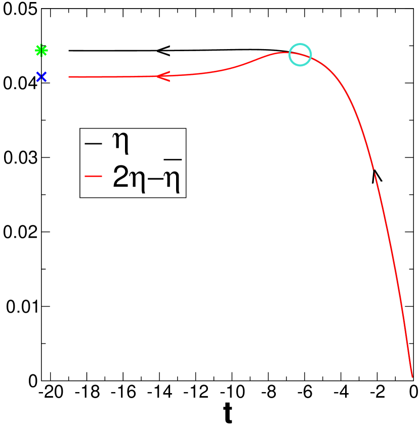
Figure 2: NP-FRG flow of the running exponent $\eta_{k}$ and of $2\eta_{k}-\bar{\eta}_{k}$ as a function of $t=\log(k/\Lambda)$ for the RFIM in $d=5$. The arrows indicate the flow toward the infrared ($k\rightarrow 0$). Note that one reaches $t\sim-19$, which means a length scale bigger than $10^{8}$ times the microscopic one. One is then clearly in the asymptotic regime as shown by comparing the curves with the symbols on the $y$-axis, which are the values obtained by directly solving the fixed-point equation. The two curves are superimposed, implying $\bar{\eta}_{k}=\eta_{k}$, until the Larkin scale (marked by a circle), at which point they separate. However, the fixed point values are such that $2\eta-\bar{\eta}$ is unambiguously strictly greater than zero.

We also plot in Fig. 3 the fixed-point value of the ratio $(2\eta-\bar{\eta})/\eta$ as a function of $d$ for the RFIM in the vicinity of $d_{DR}$ from the NP-FRG equations.footnote0 The crux of the present demonstration is not the actual values of the exponents (which, however, are always within 10$\%$ of the best estimates), but the fact that, around $d_{DR}$, $\bar{\eta}$ and $\eta$ are equal or close to each other so that $(2\eta-\bar{\eta})/\eta$ stays near 1 and unambiguously violates the prediction of the two-exponent scenario. This is clearly seen in Fig. 3.

This conclusion is similar to that reached above for the RF$O(N)$M with continuous symmetry near $d=4$ and it may actually be extended through the NP-FRG to the whole $(N,d)$ domaintissier06 (note that the approximate nonperturbative truncation of the exact FRG equations gives back the exact perturbative FRG treatment in $d=4+\epsilon$ at one loop).

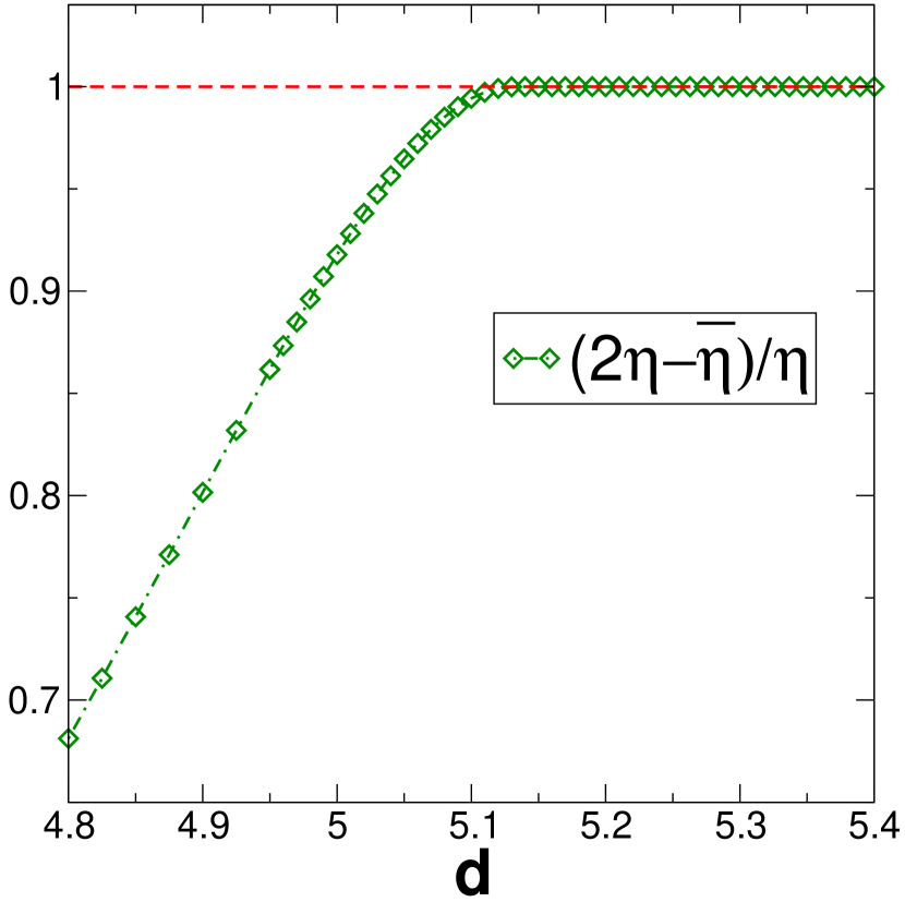
Figure 3: Ratio $(2\eta-\bar{\eta})/\eta$ as a function of $d$ for the RFIM in the vicinity of $d_{DR}\simeq 5.1$ from the NP-FRG. Above $d_{DR}$, the ratio is exactly equal to 1 as the stable fixed point is associated with the $d\rightarrow d-2$ dimensional reduction. For $d<d_{DR}$, the stable fixed point is characterized by the existence of a cusp in the cumulants of the renormalized random field. The ratio then decreases continuously from 1 as one decreases $d$. As in Fig. 1, there is a finite domain of $d$ for which $2\eta-\bar{\eta}\neq 0$ with no ambiguity.

VI Conclusion

In this paper, we have challenged the two-exponent scaling scenario of the critical behavior of random-field systems proposed by Schwartz and coworkers.schwartz85 ; schwartz86 Due to the generality of its derivations, this scenario is supposed to apply to all random field models, whether in the Ising or in the $O(N)$ version, and in all dimensions $d$ between the lower and the upper critical ones. We have however clearly proven that the predictions, most notably the relation between exponents $\bar{\eta}=2\eta$, cannot be exact for generic random-field systems.footnote1 Our proof is beyond error bars as it involves the fact that there is a whole domain of $d$ and $N$, including the Ising version, for which instead $\bar{\eta}=\eta\neq 0$ and that near the boundary of this domain the exponents verify $\bar{\eta}\simeq\eta\neq 2\eta$.

We have pointed out that a potential caveat of the derivations of the two-exponent scaling, which imply that the random-field strength is not renormalized by fluctuations at criticality, is that they are blind to rare events, regions or samples that are known to play an important role in random-field systems. The arguments leading to two-exponent scaling however apply to random-field systems with long-range correlated disorder. In such systems, the bare variance of the random field is no longer given by Eq. (2) but is characterized by an exponent $\rho$:

$$\overline{h^{\mu}(x)h^{\nu}(y)}\sim\Delta_{B}\frac{\delta_{\mu\nu}}{|x-y|^{d-\rho}}\,.$$ (12)

The long-range piece of the second cumulant of the random field is then not renormalized by fluctuations.bray86b ; fedorenko07 ; baczyk13 In this case, one therefore rigorously has that $2\eta-\bar{\eta}=\rho$. This is for instance correctly given by the heuristic derivation leading to Eq. (9) as the mean random field in a finite system scales as $L^{-(d-\rho)/2}$. Similarly, a generalization of Eq. (8) is now also valid.

In the case of the short-range RFIM, the two-exponent scaling description is exact close to the lower and (more trivially) upper critical dimensions. It moreover appears to provide an extremely good approximation in between, with $2\eta-\bar{\eta}\sim 10^{-2}$ or less. In the light of our results, this implies that computer simulations, even elaborate and extensive ones as the recent study in [fytas13, ], will likely be always inconclusive due to unavoidable residual errors.footnote2

References

- (1) Y. Imry and S. K. Ma, Phys. Rev. Lett. 35, 1399 (1975).
- (2) For a review, see T. Nattermann, Spin glasses and random fields (World scientific, Singapore, 1998), p. 277.
- (3) J. Villain, Phys. Rev. Lett. 52, 1543 (1984).
- (4) D. S. Fisher, Phys. Rev. Lett. 56, 416 (1986).
- (5) A. Aharony, Y. Imry, and S. K. Ma, Phys. Rev. Lett. 37, 1364 (1976).
- (6) G. Grinstein, Phys. Rev. Lett. 37, 944 (1976).
- (7) A. P. Young, J. Phys. C 10, L257 (1977).
- (8) G. Parisi and N. Sourlas, Phys. Rev. Lett. 43, 744 (1979).
- Imbrie (1984) J. Z. Imbrie, Phys. Rev. Lett. 53, 1747 (1984).
- Bricmont and Kupianen (1987) J. Bricmont and A. Kupianen, Phys. Rev. Lett. 59, 1829 (1987).
- (11) G. Tarjus and M. Tissier, Phys. Rev. Lett. 93, 267008 (2004); Phys. Rev. B 78, 024203 (2008).
- (12) M. Tissier and G. Tarjus, Phys. Rev. Lett. 96, 087202 (2006); ; Phys. Rev. B 78, 024204 (2008).
- (13) M. Tissier and G. Tarjus, Phys. Rev. Lett. 107, 041601 (2011); Phys. Rev. B 85, 104202 (2012); ibid 85, 104203 (2012).
- (14) G. Tarjus, M. Baczyk, and M. Tissier, arXiv:1209.3161, to appear in Phys. Rev. Lett. (2013).
- (15) M. Schwartz, J. Phys. C: Solid State Phys. 18, 135 (1985).
- (16) M. Schwartz and A. Soffer, Phys. Rev. B 33, 2059 (1986). M. Schwartz, M. Gofman and T. Natterman, Physica A 178, 6 (1991).
- (17) K. Eischhorn and K. Binder, J. Phys.: Condens. Matter 8, 5209 (1996); R. L. C. Vink, K. Binder, and H. L wen, J. Phys.: Condens. Matter 20, 404222 (2008); R. L. C. Vink, T. Fischer, and K. Binder, Phys. Rev. E 82, 051134 (2010).
- Parisi (1984) G. Parisi, in Proceedings of Les Houches 1982, Session XXXIX, edited by J. B. Zuber and R. Stora (North Holland, Amsterdam, 1984), p. 473.
- (19) N. G. Fytas and V. Martin-Mayor, preprint arXiv:1304.0318 (2013).
- (20) A. J. Bray and M. A. Moore, J. Phys. C: Solid State Phys. 18, L927 (1985).
- (21) M. Gofman, J. Adler, A. Aharony, A. B. Harris, and M. Schwartz, Phys. Rev. Lett. 71, 1569 (1993).
- (22) D. S. Fisher, Phys. Rev. B 31, 7233 (1985).
- (23) D. E. Feldman, Int. J. Mod. Phys. B 15, 2945 (2001).
- (24) P. Le Doussal and K.J. Wiese, Phys. Rev. Lett. 96, 197202 (2006).
- (25) M. Tissier and G. Tarjus, Phys. Rev. B 74, 214419 (2006).
- (26) M. Baczyk, M. Tissier, G. Tarjus, and I. Balog, unpublished (2013).
- (27) A. J. Bray and M. A. Moore, J. Phys. C 17, L463 (1984).
- (28) D. S. Fisher and D. A. Huse, Phys. Rev. B 38, 373 (1988); Phys. Rev. B 38, 386 (1988).
- (29) D. S. Fisher, Phys. Rev. Lett. 56, 1964 (1986). O. Narayan and D. S. Fisher, Phys. Rev. B 46, 11520 (1992).
- (30) L. Balents, J. P. Bouchaud, and M. Mézard, J. Phys. I 6, 1007 (1996).
- (31) P. Le Doussal, K. J. Wiese, and P. Chauve, Phys. Rev. B 66, 174201 (2002); Phys. Rev. E 69, 026112 (2004).
- (32) L. Balents and P. Le Doussal, Ann. Phys. 315, 213 (2005).
- (33) P. Le Doussal and K. J. Wiese, Phys. Rev. E 79, 051106 (2009).
- (34) P. Le Doussal, A. A. Middleton, and K. J. Wiese, Phys. Rev. E 79, 050101 (2009).
- (35) P. Le Doussal, Ann. Phys. 325, 49 (2010).
- (36) A. J. Bray, J. Phys. C: Solid State Phys. 19, 6225 (1986).
- (37) A. A. Fedorenko and F. Kuehnel, Phys. Rev. B 75, 174206 (2007).
- (38) M. Baczyk, M. Tissier, G. Tarjus, and Y. Sakamoto, arXiv:1303.2053 (2013).
- (39) Y. Sakamoto, H. Mukaida, and C. Itoi, Phys. Rev. B 74, 064402 (2006).
- (40) Note that in the case of the RFIM, and appear essentially indistinguishable.baczyk13b The difference could only affect a very small region near with no consequences on the present demonstration.
- (41) On the other hand, the Schwartz-Soffer inequality, ,schwartz-soffer85 which has a rigorous basis, is of course not questioned here.
- (42) M. Schwartz and A. Soffer, Phys. Rev. Lett. 55, 2499 (1985).
- (43) For instance, a recent extensive numerical study of the critical behavior of the 3- RFIM via ground-state determination at ,fytas13 states that . Our contention is that this does not prove, nor actually disprove, that despite the very small value.