Atomistic modeling of dynamical quantum transport

Abstract

We present dynamical transport calculations based on a tight-binding approximation to adiabatic time-dependent density functional theory (TD-DFTB). The reduced device density matrix is propagated through the Liouville-von Neumann equation. For the model system, 1,4-benzenediol coupled to aluminum leads, we are able to confirm the equality of the steady state current resulting from a time-dependent calculation to a static calculation in the conventional Landauer framework. We also investigate the response of the junction subjected to alternating bias voltages with frequencies up to the optical regime. Here we can clearly identify capacitive behaviour of the molecular device and a significant resonant enhancement of the conductance. The results are interpreted using an analytical single level model comparing the device transmission and admittance. In order to aid future calculations under alternating bias, we shortly review the use of Fourier transform techniques to obtain the full frequency response of the device from a single current trace.

1 Introduction

The field of quantum transport at the molecular scale significantly diversified over the last years [1, 2, 3]. While the interest was initially to measure the conductance across individual molecules in an accurate and reproducible fashion, current topics involve spin transport [4], molecular transistors [5], thermoelectric effects [6, 7] and device heating [8, 9]. On the theoretical side much progress was achieved using Green’s function methods in the energy domain [10]. Time domain methods, on the contrary, promise easy access to dynamical properties, like ac transport, light-induced effects and higher harmonics in the current [11]. In this contribution we report on results of such a method based on approximate time-dependent density functional theory, termed TD-DFTB [12, 13]. The scheme allows to perform dynamical transport simulations of realistic devices taking the electronic structure of molecule and leads into full account. Extending an earlier study on a similar topic [14], we first ask the question whether time and energy domain methods provide the same answer for the steady state dc current. We continue with a discussion of alternate currents and focus here especially on resonant enhancement of the admittance beyond the low frequency regime commonly studied.

2 Method

In the following we present a brief description of our simulation method. A more detailed derivation and justification of the present scheme may be found in the original articles [15] and [13]. We assume a setup of the molecular electronic device as depicted in Fig. 1. The periodic left (L) and right (R) lead extend to infinity and are in thermal equilibrium at the chemical potential $\mu_{\alpha=L,R}$ with $\mu_{L}=\mu_{R}$ at $t=0$. At $t>0$, a time-dependent bias potential $V(t)$ is applied that drives the central device region (D) out of equilibrium and leads to a time-dependent current. Instead of working with the full infinite system, one can derive a Liouville equation for the device region only [15] (in atomic units):

$$i\frac{\partial}{\partial t}\sigma(t)=[H(t),\sigma(t)]-i\sum_{\alpha=L,R}Q_{\alpha}(t).$$ (1)

Here ${\sigma(t)}$ denotes the one-particle density matrix for the device region in a basis of localized atom-centered basis functions $\phi_{\mu}(\vec{r})$. The Hamiltonian $H(t)$ is given in the adiabatic approximation of TDDFT [16] and depends on the electron density $\rho(\vec{r},t)$, while $Q_{\alpha}(t)$ incorporates all effects due to the metallic leads, especially also dephasing and dissipation. Numerically tractable and explicit forms for this term can be obtained from non-equilibriums Green’s function theory in the wide band limit (WBL). As shown by Zheng et al. [15], $Q_{\alpha}$ then takes the form:

$$Q_{\alpha}(t)=i[\Lambda_{\alpha},\sigma(t)]+\{\Gamma_{\alpha},\sigma(t)\}+K_{\alpha}(t),$$ (2)

where $\Lambda_{\alpha}$ describes the change of the device energy levels due to the presence of lead $\alpha$, while $\Gamma_{\alpha}$ renders the lifetime of the molecular levels finite. Both matrices are evaluated from first principles and depend on the device-lead interaction and the lead surface density of states. The term $K_{\alpha}$ involves only known quantities besides the time-dependent bias potential $V(t)$ and hence Eq. 1 represents a closed equation that can be numerically integrated by conventional Runge-Kutta methods. To this end, the initial density matrix at $t=0$ may be obtained without further approximations from equilibrium Green’s function theory in the WBL. As also shown in reference [15], knowledge of $Q_{\alpha}(t)$ allows one to compute the time-dependent particle current $I_{\alpha}(t)$ through the left or right device-lead interface according to

$$I_{\alpha}(t)=-\text{Tr}[Q_{\alpha}(t)].$$ (3)

In practical simulations the time step has to be chosen in the attosecond regime in order to resolve the electron dynamics accurately. This limits the accessible device dimensions and total simulation time significantly. We therefore adapted the scheme from above to the time-dependent density functional based tight-binding (TD-DFTB) method [17, 12, 13]. In essence, the TDDFT Hamiltonian matrix $H_{\mu\nu}(t)$ is replaced by

$$H_{\mu\nu}(t) = \langle\phi_{\mu}|H[\rho_{0}]|\phi_{\nu}\rangle$$

$$+ \frac{1}{2}[\delta V_{A}(t)+\delta V_{B}(t)]S_{\mu\nu},\quad\mu\in A,\nu\in B.$$

The first term on the right hand side is the DFT Hamiltonian evaluated at a time independent reference density $\rho_{0}=\sum_{A}\rho_{A}$, taken to be a sum of atomic densities $\rho_{A}$ for each atom in the device region. These densities and hence also the matrix elements can be computed beforehand. The second term involves the overlap $S_{\mu\nu}$ of the basis functions and takes the deviation of the electrostatic potential from the reference into account. The potential $V_{A}$ on the atoms in the device region is computed at each time step from a Poisson equation with boundary conditions determined by the given bias potential in the leads. The charge density required in this process is computed from the density matrix $\sigma(t)$ [13]. Besides this adaption in the Hamiltonian, we follow the formalism of Zheng et al. without further modifications.

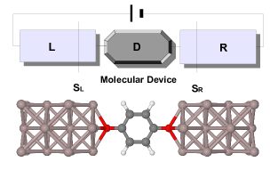
Figure 1: Schematic setup of the molecular device shown together with our test system. Only the atoms in the device region are shown.

3 Results

3.1 Approach to steady state

We applied the TD-DFTB scheme to the junction depicted in Fig. 1. The 1,4-benzenediol molecule was optimized with passivating hydrogens in vacuum at the DFTB level and then symmetrically positioned inbetween Al nanowires of finite cross sections. The device region consists of the molecule and 36 additional Al atoms, while the simulation cell for the leads included 72 atoms. The latter is periodically replicated to $+\infty$ and $-\infty$ for the right and left lead, respectively, in order to compute the surface Green’s function and WBL parameters (see Eq. 2) at zero bias. The basis set is given by one s-type atomic orbital for H and one s-type and three p-type orbitals for the other elements. The Perdew-Burke-Ernzerhof exchange-correlation functional [18] is used in all calculations. This model structure was already used in [13] as well as in the first principles TDDFT study [14], so that benchmark data is available for comparison. Transport through benzenediol is typical for conjugated molecules in many respects. The transmission at the Fermi energy $E_{F}$ is rather small (T $\approx$ 0.01) and transport occurs through the tails of the $\pi$ and $\pi^{*}$ frontier orbitals.

In Fig. 2 we plot the time-dependent current through the left and right molecule-lead interface. Here and in the following we integrate Eq. 1 with a time step of 2 as using a 4-th order Runge-Kutta method. The bias voltage of 3.5 V is applied to the left lead only and turned on exponentially with a time constant of 0.5 fs. The current initially overshoots, oscillates and settles into the steady state only after several fs, long after the bias potential nearly reached its maximum. Earlier we have shown [13], that the initial transients depend on the time constant of the exponential turn on, but not the asymptotic value of the current. In addition, we could relate the decay time of the oscillations to the imaginary part of the self energy of the device. Well coupled junctions reach the steady state earlier, whereas weakly coupled junctions feature persistent oscillations (see also [19]). As can also be seen in Fig. 2, the absolute values of the currents through the left and right interface equal each other asymptotically, but not in the transient phase of the simulation. Indeed, the particle current is a conserved quantity only in the dc limit. Under ac driving the device may become charged and one has to consider both particle current and displacement current [20]. By monitoring the total device charge as a function of time, we verified that the latter indeed compensates for the difference between $|I_{L}(t)|$ and $|I_{R}(t)|$.

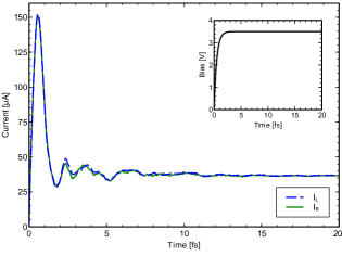
Figure 2: Absolute value of the time-dependent current through the left ($I_{L}$) and right ($I_{R}$) interface of the molecular junction depicted in Fig. 1. The inset shows the bias potential $V(t)=V_{0}[1-\exp(-t/T)]$ with $V_{0}=3.5$ V and $T=0.5$ fs.

An interesting question is now, whether the asymptotic current $I_{\text{TD}}^{\infty}=\lim_{t\to\infty}I(t)$ from the time-dependent simulation equals the current obtained from a conventional static calculation in the Landauer formalism. In the latter approach the current is given by the energy integral

$$I=G_{0}\int_{-\infty}^{\infty}dE\left[f(E,\mu_{L})-f(E,\mu_{R})\right]\,T(E,V)$$

$$T(E,V)={\rm Tr}\left[G^{r}\Gamma_{R}G^{a}\Gamma_{L}\right],$$ (5)

with $f(E,\mu)$ denoting Fermi distribution functions with $\mu_{L}-\mu_{R}=V$, the quantum of conductance $G_{0}\approx 77.48\mu$S, and the bias dependent transmission function $T(E,V)$ [10]. The retarded ($G^{r}$) and advanced ($G^{a}$) device Green’s functions depend on the Hamiltonian and charge density n(r). Since n(r) depends itself on $G^{r}$ as well as on the applied bias, a self-consistent determination of all quantities is required. It is not a-priori evident, that the currents given by Eq. 3 and Eq. 5 are identical. We have recently discussed this question in great detail in the context of first-principles TDDFT [14]. Here we perform similar simulations using the TD-DFTB method in order to show that our findings are not restricted to a specific choice of the Hamiltonian. In Fig. 3 we compare the asymptotic currents $I_{\text{TD}}^{\infty}$ from several time-dependent simulations at different bias values with the corresponding values from Eq. 5. Despite significant formal and also algorithmic differences between the two approaches, one can observe nearly identical values over the full bias range. Like in Ref. [14], we conclude that time-dependent simulations do in general not offer additional or more accurate information when the interest is in steady state properties. As we discuss in the next section, there is however an important computational advantage for ac transport.

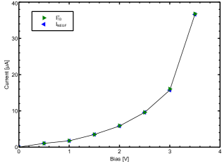
Figure 3: Asymptotic time-dependent current ($I_{\text{TD}}^{\infty}$) and current in the Landauer formalism ($I_{\text{NEGF}}$) for 1,4-benzenediol as a function of applied bias. The values for $I_{\text{TD}}^{\infty}$ have been obtained from simulations with a total simulation time $t_{\text{max}}$ of 20 fs and a bias potential $V(t)=V_{0}[1-\exp(-t/T)]$ with T= 0.5 fs. The current has been averaged over the last 2 fs. The wide band approximation was also employed in the Landauer calculations. The line is a guide to the eye.

3.2 Admittance from current traces

Starting with the work of Fu and Dudley [24], several studies addressed the response of meso- and nanoscopic devices to an alternating bias potential [25, 26, 27]. In recent years approaches based on energy domain Green’s functions became especially popular [28, 29, 30, 31], but also time domain techniques, as presented here, allow for the efficient evaluation of the admittance [32].

To this end, the Fourier transform of bias and current is numerically evaluated, e.g.,

$$V(\omega)=\int_{-\infty}^{\infty}V(t)\exp(i\omega t)dt$$ (6)

to yield the complex admittance $Y(\omega)=I(\omega)/V(\omega)$. In electronic circuit theory, the real and imaginary parts of $Y$ are also often termed conductance ($G=\text{Re}(Y)$) and suceptance ($B=\text{Im}(Y)$), respectively. With the choice for the sign of the Fourier transform from above (Eq. 6), capacitive devices feature a negative susceptance, while inductive behaviour is characterized by positive values of $B$.

We applied this approach to the 1,4-benzenediol junction and experimented with different choices for the temporal profile of the bias potential. In principle, the form of $V(t)$ is arbitrary as long as the amplitude is small enough to remain in the linear response regime and the support of its Fourier transform is sufficiently large. Fig. 4 depicts the absolute value of the admittance $|Y(\omega)|$ for different functions $V(t)$. As reference, we perform simulations with a harmonic bias $V(t)=V_{0}\sin(\omega t)$ for different discrete values of $\omega$ and determine the amplitude of $I(t)$ after the initial transients have died out. A sample simulation is shown in Fig. 5. Inspection of Fig. 4 reveals that an exponential turn-on of the form $V(t)=V_{0}[1-\exp(-t/T)]$ provides a reasonable estimate for the general features in the admittance, but fails to convince on a quantitative level. The reason is that the Fourier transform does not exist in the limit $\omega\to 0$, unless one artificially damps $V(t)$ by a factor $\exp(-\Gamma t)$ to enforce convergence. For small values of $\Gamma$ the admittance differs strongly from the reference, while for larger values the dc limit is overestimated. In response calculations for optical properties one often uses a Dirac delta function or Lorentzian as a perturbation. Here, the Fourier transform exists for all $\omega$ and no artificial broadening is required. Results for the bias potential

$$V(t)=\frac{V_{0}}{\pi}\frac{\gamma}{(t-t_{0})^{2}+\gamma^{2}},$$ (7)

show excellent agreement with the reference data over nearly the full frequency range, especially also in the dc limit. A benefit with respect to the simulations at discrete frequencies is that the Fourier transform technique requires only a single run to evaluate the full admittance. In the following we therefore continue with this choice.

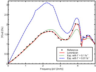
Figure 4: Absolute value of admittance $|Y(\omega)|$ in units of $G_{0}$ as a function of frequency in units of [eV/$\hbar$]. Results are given for the harmonic perturbation with discrete frequencies (Reference) and using Fourier transforms with exponential form and damping of the bias ($V_{0}=$ 1 mV, $T=$ 0.2 fs, $t_{\text{max}}=$ 50 fs) as well as with Lorentzian form ($V_{0}=$ 0.1 mV, $\gamma=$ 0.2 fs, $t_{0}=$ 2 fs, $t_{\text{max}}=$ 50 fs).

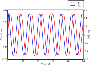
Figure 5: time-dependent current due to the ac bias $V(t)=V_{0}\sin(\omega t)$ ($V_{0}=$ 0.5 $\mu$V, $\omega=$ 0.59 eV/$\hbar$, $t_{\text{max}}=$ 50 fs).

After this more technical discussion we now analyze the admittance in more detail. Fig. 6 a) shows the conductance and susceptance of 1,4-benzenediol. For small frequencies, the negative values of the latter indicate capacitive behaviour of the junction. This is in line with the simulations shown in Fig. 5, where the current leads the voltage signal. The negative susceptance can be rationalized by inspection of the transmission T(E,0) (Fig. 6 c)) of the junction. For small frequencies, only the region around the Fermi energy is relevant in the linear response regime. Here the transmission is low and the current effectively blocked, similar to a macroscopic capacitor. In a classical RC circuit, the admittance is given by

$$Y^{\text{RC}}(\omega)=-i\omega C+\omega^{2}C^{2}R,$$ (8)

up to second order in the frequency [28]. As seen in Fig. 6 a), real and imaginary part of $Y(\omega)$ show for small frequencies indeed quadratic and linear scaling, respectively.

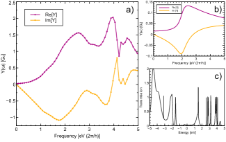
Figure 6: a) Real and imaginary part of the admittance $Y(\omega)$ for 1,4-benzenediol. b) Analytical results for the one-level model of Fu and Dudley [24] with parameters $\Delta E=$ 2 eV and $\gamma=$ 0.25 eV. c) Transmission T(E,0) of 1,4-benzenediol.

For larger frequencies, resonances appear around 2.5 eV/$\hbar$ and 4 eV/$\hbar$ with conductances that are two orders of magnitude larger than the dc one. This can be qualitatively understood by a comparison to the analytical result of Fu and Dudley for a single-level model [24], characterized by a Breit-Wigner transmission

$$T(E)=\frac{\gamma^{2}}{(E-E_{0})^{2}+\gamma^{2}},$$ (9)

where $E_{0}$ denotes the level energy. Here the admittance is given by

$$\text{Re}\{Y(\omega)\}=\\ G_{0}\frac{\gamma}{2\omega}\left[\arctan\left(\frac{\Delta E+\omega}{\gamma}\right)-\arctan\left(\frac{\Delta E-\omega}{\gamma}\right)\right]$$ (10)

and

$$\text{Im}\{Y(\omega)\}=\\ G_{0}\frac{\gamma}{4\omega}\ln\left(\frac{\left[(\Delta E+\omega)^{2}+\gamma^{2}\right]\left[(\Delta E-\omega)^{2}+\gamma^{2}\right]}{\left[\Delta E^{2}+\gamma^{2}\right]^{2}}\right),$$ (11)

with $\Delta E=E_{F}-E_{0}$. In Fig. 6 b) the Fu-Dudley admittance is shown for $\Delta E=$ 2 eV and $\gamma=$ 0.25 eV. The qualitative similarity to the atomistic results for a real junction is clearly seen. Our calculations include a large number of molecular states, while Eqs. 10 and 11 hold only for a single channel. Still a rough assignment of the resonances to individual molecular states becomes possible. The first resonance likely originates from the unoccupied states 1.5 eV above and the occupied states 2.2 eV below the Fermi energy. According to the analytical results, states with smaller broadening contribute less to the admittance. The resonance around 4 eV is therefore assigned to the broad resonance in the transmission around this energy. The underlying physical picture is that the time-dependent bias potential opens new transport channels at E+$\hbar\omega$ and E -$\hbar\omega$, which are not available in the dc limit.

Admittedly, the frequency range for resonant enhancement is difficult to access experimentally. Current measurements on nanoscopic conductors hardly reach the GHz regime [33, 34]. Nevertheless, appropriate gating of the device could move the HOMO/LUMO close to the Fermi energy, resulting in resonance enhancement at lower frequencies. Small gap materials like Graphene nanoribbons would offer another route for the experimental realization of this effect.

4 Summary

In this study, we investigated the behaviour of a contacted 1,4-benzenediol molecule subjected to an alternating bias directly and using a Fourier transform of Lorentzian and exponential voltage signals. The Lorentzian input signal led to very good agreement with reference discrete frequency calculations. In the admittance, capacitive behaviour could be identified and interpreted through the transmission of the junction. An analytical single level model showed large qualitative similarities to our numerical results. The approach we employed for these findings is a combination of the highly efficient tight-binding approximation to adiabatic TDDFT and a device density matrix propagation scheme derived within the Keldysh formalism by Zheng and co-workers. Following earlier discussions on this topic, we can also confirm that a different choice of the self-consistent Hamiltonian does not change the equality of the TD steady state with its static counterpart at the NEGF level.

Financial support by the German Science Foundation (DFG, SPP 1243 and GRK 1570) is greatly acknowledged.

References

- [1] A. Nitzan, M. A. Ratner, Electron transport in molecular wire junctions, Science 300 (5624) (2003) 1384–1389.
- [2] J. R. Heath, Molecular electronics, Annu. Rev. Mater. Res. 39 (2009) 1–23.
- [3] R. L. McCreery, H. Yan, A. J. Bergren, A critical perspective on molecular electronic junctions: there is plenty of room in the middle, Phys. Chem. Chem. Phys. 15 (4) (2013) 1065–1081.
- [4] L. Bogani, W. Wernsdorfer, Molecular spintronics using single-molecule magnets, Nat. Mater. 7 (3) (2008) 179–186.
- [5] H. Song, Y. Kim, Y. H. Jang, H. Jeong, M. A. Reed, T. Lee, Observation of molecular orbital gating, Nature 462 (7276) (2009) 1039–1043.
- [6] P. Reddy, S.-Y. Jang, R. A. Segalman, A. Majumdar, Thermoelectricity in molecular junctions, Science 315 (5818) (2007) 1568–1571.
- [7] B. K. Nikolić, K. K. Saha, T. Markussen, K. S. Thygesen, First-principles quantum transport modeling of thermoelectricity in single-molecule nanojunctions with graphene nanoribbon electrodes, Journal of Computational Electronics 11 (2012) 1–15.
- [8] A. Gagliardi, G. Romano, A. Pecchia, A. Di Carlo, T. Frauenheim, T. A. Niehaus, Electron-phonon scattering in molecular electronics: from inelastic electron tunnelling spectroscopy to heating effects, New J. Phys. 10 (2008) 065020.
- [9] G. Schulze, K. J. Franke, A. Gagliardi, G. Romano, C. Lin, A. Da Rosa, T. A. Niehaus, T. Frauenheim, A. Di Carlo, A. Pecchia, J. I. Pascual, Resonant electron heating and molecular phonon cooling in single c60 junctions, Phys. Rev. Lett. 100 (2008) 136801.
- [10] J. C. Cuevas, E. Scheer, Molecular Electronics: An Introduction to Theory and Experiment, World Scientific, 2010.
- [11] G. Chen, T. Niehaus, Quantum Simulation for Material and Biological systems, Springer, 2012, Ch. Quantum transport simulations based on time dependent density functional theory, pp. 17–32.
- [12] T. A. Niehaus, Approximate time-dependent density functional theory, J. Mol. Struct.: THEOCHEM 914 (2009) 38.
- [13] Y. Wang, C.-Y. Yam, T. Frauenheim, G. Chen, T. Niehaus, An efficient method for quantum transport simulations in the time domain, Chem. Phys. 391 (1) (2011) 69.
- [14] C. Y. Yam, X. Zheng, G. H. Chen, Y. Wang, T. Frauenheim, T. A. Niehaus, Time-dependent versus static quantum transport simulations beyond linear response, Phys. Rev. B 83 (2011) 245448.
- [15] X. Zheng, F. Wang, C. Y. Yam, Y. Mo, G. H. Chen, Time-dependent density-functional theory for open systems, Phys. Rev. B 75 (19) (2007) 195127.
- [16] M. E. Casida, Recent Advances in Density Functional Methods, Part I, World Scientific, 1995, Ch. Time-dependent Density Functional Response Theory for Molecules, pp. 155–192.
- [17] T. Frauenheim, G. Seifert, M. Elstner, T. Niehaus, C. Kohler, M. Amkreutz, M. Sternberg, Z. Hajnal, A. Di Carlo, S. Suhai, Atomistic simulations of complex materials: ground-state and excited-state properties, Journal Of Physics-Condensed Matter 14 (11) (2002) 3015–3047.
- [18] J. Perdew, K. Burke, M. Ernzerhof, Generalized gradient approximation made simple, Phys. Rev. Lett. 77 (18) (1996) 3865–3868.
- [19] E. Khosravi, S. Kurth, G. Stefanucci, E. K. U. Gross, The role of bound states in time-dependent quantum transport, Appl. Phys. A 93 (2) (2008) 355–364.
- [20] B. Wang, J. Wang, H. Guo, Current partition: A nonequilibrium green’s function approach, Phys. Rev. Lett. 82 (2) (1999) 398–401.
- [21] F. Evers, F. Weigend, M. Koentopp, Conductance of molecular wires and transport calculations based on density-functional theory, Phys. Rev. B 69 (23) (2004) 235411.
- [22] N. Sai, M. Zwolak, G. Vignale, M. Di Ventra, Dynamical corrections to the dft-lda electron conductance in nanoscale systems, Phys. Rev. Lett. 94 (18) (2005) 186810.
- [23] G. Vignale, M. Di Ventra, Incompleteness of the landauer formula for electronic transport, Phys. Rev. B 79 (1) (2009) 14201.
- [24] Y. Fu, S. Dudley, Quantum inductance within linear response theory, Phys. Rev. Lett. 70 (1) (1993) 65–68.
- [25] A. Jauho, N. Wingreen, Y. Meir, Time-dependent transport in interacting and noninteracting resonant-tunneling systems, Phys. Rev. B 50 (8) (1994) 5528.
- [26] T. Christen, M. Büttiker, Low frequency admittance of a quantum point contact, Phys. Rev. Lett. 77 (1996) 143–146.
- [27] R. Baer, T. Seideman, S. Ilani, D. Neuhauser, Ab initio study of the alternating current impedance of a molecular junction, J. Chem. Phys. 120 (2004) 3387.
- [28] Y. Yu, B. Wang, Y. Wei, Corrected article: “ac response of a carbon chain under a finite frequency bias” [j. chem. phys. [bold 127], 104701 (2007)], J. Chem. Phys. 127 (16) (2007) 169901.
- [29] T. Yamamoto, K. Sasaoka, S. Watanabe, Universal transition between inductive and capacitive admittance of metallic single-walled carbon nanotubes, Phys. Rev. B 82 (20) (2010) 205404.
- [30] T. Sasaoka, K.and Yamamoto, S. Watanabe, K. Shiraishi, ac response of quantum point contacts with a split-gate configuration, Phys. Rev. B 84 (2011) 125403.
- [31] D. Hirai, T. Yamamoto, S. Watanabe, Theoretical analysis of ac transport in carbon nanotubes with a single atomic vacancy: Sharp contrast between dc and ac responses in vacancy position dependence, Applied Physics Express 4 (7) (2011) 075103.
- [32] C. Y. Yam, Y. Mo, F. Wang, X. Li, G. H. Chen, X. Zheng, Y. Matsuda, J. Tahir-Kheli, A. G. William III, Dynamic admittance of carbon nanotube-based molecular electronic devices and their equivalent electric circuit, Nanotech. 19 (2008) 495203.
- [33] J. Plombon, K. P. OBrien, F. Gstrein, V. M. Dubin, Y. Jiao, High-frequency electrical properties of individual and bundled carbon nanotubes, Appl. Phys. Lett. 90 (6) (2007) 063106–063106.
- [34] K. Yamauchi, S. Kurokawa, A. Sakai, Admittance of au/1, 4-benzenedithiol/au single-molecule junctions, Appl. Phys. Lett. 101 (25) (2012) 253510–253510.