Energy Density Bounds in Cubic Quasi-Topological Cosmology

U. Camara dS^∗, A.A. Lima^∗ and G.M.Sotkov^∗

${}^{*}\;$Departamento de Física - CCE
Universidade Federal do Espírito Santo
29075-900, Vitória - ES, Brazil

ABSTRACT

We investigate the thermodynamical and causal consistency of cosmological models of the cubic Quasi-Topological Gravity (QTG) in four dimensions, as well as their phenomenological consequences. Specific restrictions on the maximal values of the matter densities are derived by requiring the apparent horizon’s entropy to be a non-negative, non-decreasing function of time. The QTG counterpart of the Einstein-Hilbert (EH) gravity model of linear equation of state is studied in detail. An important feature of this particular QTG cosmological model is the new early-time acceleration period of the evolution of the Universe, together with the standard late-time acceleration present in the original EH model. The QTG correction to the causal diamond’s volume is also calculated.

KEYWORDS: Cubic Quasi-Topological Gravity, Effective EoS, Entropic bounds, Causal Entropic Principle.

1 Introduction

Regions containing extremely dense matter are a common feature of all the big-bang inflationary cosmological space-times. The consistent description of such high energy states in the evolution of the Universe requires certain “higher curvature” extensions of Einstein-Hilbert (EH) gravity, involving powers (of the traces) of the Riemann tensor, believed to take into account the short distance quantum effects. Such corrections to the EH action are known to arise as counter-terms in the perturbative quantization both of matter in curved spaces [1] and of pure EH gravity as well [2, 3]. The main problem with “higher curvature” gravity theories concerns the presence of higher derivatives of the metric in the equations of motion, which in general lead to causal and unitarity inconsistencies [2, 3] when considered out of the framework of superstring theory. Nevertheless, the extensive studies of such models, in particular the so called modified $f(R)$-gravities, have found interesting applications in different areas of modern cosmology (see, e.g., [4, 5, 6] and references therein).

The present paper is devoted to the investigation of the effects caused by the higher curvature terms in a particular cosmological model in four dimensions, based on the simplest “most physical” extended gravity, given by the following cubic action for Quasi-Topological Gravity [7]:

$$S_{\mathrm{GBL}}=\int\!\frac{\sqrt{-g}\,{\mathrm{d}}^{4}x}{\varkappa^{2}}\Big{\{}R-\lambda L^{2}\left[2R^{2}-8R_{\alpha\beta}R^{\alpha\beta}+2R_{\alpha\beta\mu\nu}R^{\alpha\beta\mu\nu}\right]$$

$$+\frac{\mu L^{4}}{4}\Big{[}R^{3}+18R^{\alpha\beta\gamma\delta}R_{\gamma\delta\mu\nu}R^{\mu\nu}{}{}_{\alpha\beta}-40R^{\alpha\beta}{}_{\gamma\delta}R^{\gamma\mu}{}{}_{\beta\nu}R^{\delta\nu}{}_{\alpha\mu}$$

$$-36R^{\alpha\beta\gamma\delta}R_{\alpha\gamma}R_{\beta\delta}+8R^{\alpha\beta}R_{\beta\gamma}R^{\gamma}{}_{\alpha}\big{]}+{\mathcal{L}}_{\mathrm{matter}}\big{\}},$$ (1)

where $\varkappa^{2}\equiv 16\pi G=4l_{{\mathrm{Pl}}}^{2}$; $l_{\mathrm{Pl}}$ is the Planck length; $\lambda$, $\mu$ are dimensionless “gravitational coupling” constants, while $L$ is a new length scale, which can be chosen as $L=l_{\mathrm{Pl}}$ by an appropriate redefinition of $\lambda$ and $\mu$. We include the cosmological constant $\Lambda_{0}>0$ implicitly in the matter Lagrangian ${\mathcal{L}}_{\mathrm{matter}}$.

The remarkable feature of this cubic extension of the EH action, is that the corresponding equations of motion for all conformally flat metrics, as for example those of domain walls and of flat Friedmann-Robertson-Walker (FRW) space-times:

$${\mathrm{d}}s^{2}=-{\mathrm{d}}t^{2}+a^{2}(t)\,{\mathrm{d}}x^{i}{\mathrm{d}}x_{i}\;,$$ (2)

are of second order [8], while arbitrary metrics yield, in general, equations of motion of fourth order. This fact, together with the introduction of an appropriate superpotential and the related BPS-like first order system of equations for the cubic QTG-matter model (1), derived in Ref.[8], provide an efficient method for the analytic construction of a large family of exact flat FRW’s solutions, representing asymptotically ${\mathrm{dS}}_{4}$ space-times.

The most important and universal new property of these higher curvature cosmological models is that, differently from the EH case, the entropy prescribed to the apparent horizons [9]

$$s(t)=\frac{16\pi^{2}}{\varkappa^{2}}\,\frac{1}{H^{2}}\left(1-2\lambda L^{2}\,H^{2}+3\mu L^{4}\,H^{4}\right)\,$$ (3)

with $H\equiv\dot{a}/a$ denoting the Hubble factor, is not automatically positive definite and increasing. As a consequence, the requirement of the thermodynamical consistency of these models: $s(t)\geq 0$ and ${\mathrm{d}}s/{\mathrm{d}}t>0$, introduces certain restrictions on the available maximal values $\varrho_{\max}$ of the matter densities $\varrho=\frac{6}{\varkappa^{2}}H^{2}\leq\varrho_{\max}$ and certain minimal scales $L_{\min}$ (related to $\varrho_{\max}$) up to which we can have a physically meaningful description of the Universe evolution within the framework of the cubic QTG cosmologies.

In order to exemplify the effects caused by the higher curvature terms, we choose a particularly simple and yet quite rich cosmological model, representing a QTG extension of the following EH model of a linear equation of state:

$$p_{0}/\varrho_{0}=w_{1}-w_{2}/\varrho_{0}\;.$$ (4)

The matter content is that of a barotropic fluid with constant equation of state parameter $w_{1}$, together with a dark energy “fluid” representing the cosmological constant $\Lambda_{0}=\varkappa^{2}w_{2}/2(1+w_{1})$. This EH cosmological model has been widely studied [10, 11, 12, 13], with a particularly remarkable result by Bousso et al. [10], who deduce the value of the cosmological constant for a universe dominated by dust through most of its history ($w_{1}=0$). The new QTG features established in the present paper are: The presence of a new (early-time) acceleration period; changes in the duration of the acceleration and deceleration periods, as well as of the future and past event horizon radii; and finally certain very small corrections to the volume of the causal diamond (to be compared with the EH one [10]).

2 Modified FRW Cosmology

Consider an universe filled with a barotropic fluid with energy density $\varrho_{0}$ and pressure $p_{0}$, components of a ‘bare’ energy-momentum matter-tensor $T^{(0)}_{\mu\nu}$. For the ansatz (2), the QTG equations of motion derived from (1) are the modified Friedmann equations:

$$\varkappa^{2}\varrho_{0}=6H^{2}\left(1-\mu L^{4}\,H^{4}\right)\;,$$ (5a)

$$\varkappa^{2}(\varrho_{0}+p_{0})=-4\dot{H}\left(1-3\mu L^{4}\,H^{4}\right)\;;$$ (5b)

$$\dot{\varrho}_{0}+3H(p_{0}+\varrho_{0})=0\;.$$ (5c)

They reduce to the usual EH-Friedmann equations when $\mu=0$; otherwise the contributions from the QTG terms may be regarded as separating a “gravitational energy momentum tensor” $T^{{\mathrm{QTG}}}_{\mu\nu}$ at the right-hand side of the Einstein equations, thus composing an effective energy momentum tensor $T^{\mathrm{eff}}_{\mu\nu}$, viz.

$$G_{\mu\nu}=T^{\mathrm{eff}}_{\mu\nu}\;;\quad T^{\mathrm{eff}}_{\mu\nu}=T^{(0)}_{\mu\nu}+T^{{\mathrm{QTG}}}_{\mu\nu},$$

where $G_{\mu\nu}$ is the Einstein tensor. Notice that the effective energy-momentum tensor has all the properties of a perfect fluid tensor, i.e. its components, $T^{\mathrm{eff}}_{\mu\nu}={\mathrm{Diag}}\;(-\varrho,p,p,p)$ satisfy the usual, EH Friedmann equations:

$$\varrho=\frac{6}{\varkappa^{2}}H^{2},\quad\varrho+p=-\frac{4}{\varkappa^{2}}\dot{H}\;,$$ (6)

as well as the continuity equation,

$$\dot{\varrho}+3H(p+\varrho)=0\;,$$ (7)

which is a simple consequence of the Bianchi identities. Because of its direct connection to the Hubble function, the cosmological observations (of distances and red shifts) should perceive not the bare energy density $\varrho_{0}$, but rather the effective one, $\varrho$, related to the former via Eq.(5a):

$$\varrho_{0}=\varrho\left(1-\mu L^{4}\frac{\varkappa^{4}}{36}\varrho^{2}\right)\;.$$ (8)

Although such a hydrodynamical interpretation of $T^{\mathrm{eff}}_{\mu\nu}$ is rather formal, we further assume that this “effective fluid” obeys the weak energy condition, i.e. $p+\varrho\geq 0$, what assures that $\dot{H}\leq 0$. Then if the bare fluid also satisfies the weak energy condition, the function

$$C_{0}\equiv 1-3\mu L^{4}\,H^{4}=1-\frac{1}{12}\mu L^{4}\varkappa^{4}\varrho^{2}$$ (9)

must be positive (or vanishing), as can be seen from Eq.(5b). While this condition holds automatically for $\mu\leq 0$, for positive values of $\mu$ the sign of $C_{0}$ will depend on the value of the energy density; it vanishes for $\varrho=\frac{2}{L^{2}\varkappa^{2}}\sqrt{3/\mu}$ and it is indeed negative for greater values of $\varrho$. Since near a singularity the value of $\varrho$ grows without bounds, for $\mu>0$ it is only possible that both the bare and the effective fluids satisfy the weak energy condition in a nonsingular universe. This would be the case, for example, in bounce-like models beginning and ending at de Sitter spaces with (asymptotic) densities $\varrho_{{\mathrm{dS}}}\leq\frac{2}{L^{2}\varkappa^{2}}\sqrt{3/\mu}$. We leave the study of such spaces for a more thorough discussion in [14], and focus for the remainder of this letter in the singular cases, thus considering only $\mu\leq 0$.

3 Horizon entropy

Killing event horizons are known to posses thermodynamical properties: a temperature $T$ related to the surface gravity, and an entropy $s$ which in EH gravity is given by the Bekenstein-Hawking formula $s=A/4$ (in geometrized units), $A$ being the area of the horizon [15, 16, 17]. Then the Einstein equations can be rewritten as a Clausius relation [18], ${\mathrm{d}}E=T\,{\mathrm{d}}s$, for the flux of energy ${\mathrm{d}}E$ across the horizon.

The lack of time-like Killing vectors in non-stationary space-times – as for example typical FRW spaces – represents an obstacle in the definition of a surface gravity for the corresponding dynamical apparent horizons. A possible consistent generalization of the “Thermodynamics/Gravity” correspondence can nevertheless be achieved by using the Kodama vector to define the horizon’s Kodama-Hayward temperature $T_{{\mathrm{KH}}}$ [25]. As it was recently shown by Cai et al. [21, 22], the corresponding Friedmann equations, for EH gravity and for certain modified theories as well, turn out to be again equivalent to the Clausius relation ${\mathrm{d}}E_{{\mathrm{MS}}}=T_{{\mathrm{KH}}}\,{\mathrm{d}}s_{{\mathrm{KW}}}$, with $E_{{\mathrm{MS}}}$ being the Misner-Sharp energy and $s_{{\mathrm{KW}}}$ an appropriately defined Kodama-Wald entropy, which for the cubic QTG cosmologies is given by Eq.(3). Notice that for de Sitter space-times, when $H$ is constant and the apparent horizon coincides with the Killing event horizon, our formula (3) reduces to the known static QTG Wald entropy [9].

The consistent interpretation of $s_{{\mathrm{QTG}}}(t)$, given by Eq.(3), as an entropy for the apparent horizon in the considered QTG cosmological models requires that it must be a non-negative and non-decreasing function of time. The later is always true if both effective and bare fluids do satisfy the weak energy condition. Then as a consequence we have that $\dot{s}=-\frac{3}{2G\varkappa^{2}}\,\frac{C_{0}(\varrho)}{\varrho^{2}}\,\dot{\varrho}\geq 0$. The restrictions imposed by the positivity condition $s_{{\mathrm{QTG}}}(t)\geq 0$ are slightly more involved: depending on the signs and values of $\lambda$ and $\mu$, they turn out to introduce certain upper bounds on the energy density $\varrho$.

Gauss-Bonnet Gravity: The topological nature of the GB term in the action renders the dynamics (i.e. the equations of motion) of GB gravity, for which $\mu=0$ and $\lambda\neq 0$, identical to that of EH gravity. But the horizon entropy is not simply proportional to $H^{-2}$, in fact

$$s(t)=\frac{1}{4G}\left(\frac{1}{H^{2}}-2\lambda L^{2}\right)\;.$$

Thus if $\lambda<0$ the entropy density is always positive, but for $\lambda>0$ there is a value of $H(t)$ – or, equivalently, of $\varrho$ – past which the entropy becomes negative. Therefore the assumption of positivity of entropy places as an upper boundary, $\varrho_{\mathrm{GB}}$, on the possible values of the energy density:

$$0\leq\varrho\leq\varrho_{\mathrm{GB}}\;;\quad\varrho_{\mathrm{GB}}\equiv\frac{3}{\varkappa^{2}L^{2}\lambda}\;$$ (10)

Quasi-Topological Gravity: Similar considerations applied to the QTG model, for the negative values of the coupling $\mu<0$ we are interested in, lead us to the conclusion that the apparent horizon entropy is only positive for densities within the finite interval:

$$0\leq\varrho\leq\varrho_{\mathrm{QTG}}\equiv\frac{2}{\varkappa^{2}L^{2}}\,\frac{1}{\mu}\left(\lambda-\sqrt{\lambda^{2}-3\mu}\right).$$ (11)

In a singular universe, it is then inevitable that at some instant the (divergent) effective energy density violates the entropic threshold of Eqs.(10) or (11) for a finite value of $\varrho$. Hence in the considered GB gravity (with $\lambda>0$) and QTG models of $\mu<0$, the cosmological singularity lies in a region of space-time which is already unphysical, for the apparent horizon entropy is negative.

4 An example of QTG cosmology

In order to describe the changes in the evolution of the homogeneous and isotropic Universe caused by the cubic QTG terms, we next address the problem concerning the construction of analytic solutions of the modified Friedmann equations (5) in the particular example of the matter stress-energy tensor $T^{(0)}_{\mu\nu}$, whose components are related by the following linear barotropic equation of state [10, 11, 12, 13]:

$$p_{0}/\varrho_{0}=\omega_{0}(\varrho_{0})\;;\quad\omega_{0}(\varrho_{0})=w_{1}-w_{2}/\varrho_{0}\;.$$ (12)

The constant $w_{2}$, if positive, represents an energy density which contributes to the pressure $p_{0}$ independently of the variable energy density $\varrho_{0}$ – thus when the former dominates (i.e. $w_{2}/\varrho_{0}\gg 1$), the dynamics is driven by a constant energy density with EoS $p_{0}=-w_{2}$, resulting in a de Sitter geometry. In this sense, $w_{2}$ may be identified with the cosmological constant and (12) is an example of a simple quintessence model. The constant $w_{1}$, which may be seen as the “matter EoS parameter” (as opposed to the “cosmological constant parameter” $w_{2}$) is equal to the velocity of sound in the fluid: $v_{0}^{2}=\partial p_{0}/\partial\varrho_{0}=w_{1}$ (in Plank units, $c=1=\hbar$). The causality condition $w_{1}<1$ excludes superluminal velocities, and if we also assume that the universe does not have a “phantom” phase, then we have to impose $|w_{1}|<1$.

The dynamics of the universe in such QTG cosmology may be found by solving the differential equation for $H(t)$ obtained by combining Eqs.(5) with the EoS (12):

$$(1-3\mu L^{4}H^{4})\dot{H}=-\frac{3}{2}H^{2}(1-\mu L^{4}H^{4})(1+w_{1})+\frac{\varkappa^{2}}{4}w_{2},$$ (13)

the integration of which yields

$$t(H)=-\frac{2}{3(1+w_{1})}\frac{1}{L^{4}\mu}\Bigg{\{}2\upsilon\left[{\mathrm{arc\,tg}}\left(\frac{H-\xi}{\zeta}\right)+{\mathrm{arc\,tg}}\left(\frac{H+\xi}{\zeta}\right)\right]$$

$$-\chi\log\left(\frac{(H-\xi)^{2}+\zeta^{2}}{(H+\xi)^{2}+\zeta^{2}}\right)+\frac{\alpha}{H_{\Lambda}}\,{\mathrm{arc\,cth}}\left(H/H_{\Lambda}\right)-2\pi\upsilon\Bigg{\}}.$$ (14)

Here $H_{\Lambda}^{2}$ is the only real root of the cubic equation (8) when written in terms of $H^{2}=\varkappa^{2}\varrho/6$ and solved for $H^{2}$, with $H_{0}^{2}\equiv\varkappa^{2}\varrho_{0}/6$ considered known. The real and imaginary parts of the remaining roots, $h^{2}$ and its complex conjugate $\bar{h}^{2}$, are denoted by $\xi$ and $\zeta$, while $\chi$ and $\upsilon$ are the real and imaginary parts of $\alpha/2\equiv\frac{1-3\mu L^{4}h^{4}}{2h(h^{2}-H_{\Lambda}^{2})(h^{2}-\bar{h}^{2})}$. Notice that we have chosen one specific singular solution $H(t\to 0)\to\infty$ of Eq.(13), representing big-bang space-times with singularity at $t=0$. Depending on the initial conditions imposed on $H(t)$ (or equivalently on $\varrho(t)$) one can construct other non-singular bounce-like solutions (both for QTG or EH models), which are however out of the scope of the problems discussed in the present paper.

The function $t(H)$ (14) is not trivially invertible; nevertheless it allows to describe the properties of the different periods of acceleration and deceleration of the QTG corrected Universe evolution, that can be obtained directly from Eqs.(13), (5b) and (6). We next recall that one can also use the deceleration parameter $q\equiv-\ddot{a}\,a/\dot{a}^{2}$ (for $\dot{a}\neq 0$), written in a suggestive form:

$$q=\frac{1}{2}(1+3\,p/\varrho)\;,$$ (15)

in order to determine whether the universe undergoes accelerated ($q<0$) or decelerated ($q>0$) expansion. Thus, the ratio $p/\varrho\equiv\omega_{\mathrm{eff}}$ between the components of the effective energy-momentum tensor plays the role of an ‘effective equation of state’. Its explicit form :

$$\omega_{\mathrm{eff}}(\varrho)=-1+\frac{(1+w_{1})\left(1-\mu L^{4}\varkappa^{4}\varrho^{2}/36\right)\varrho-w_{2}}{\varrho\left(1-\mu L^{4}\varkappa^{4}\varrho^{2}/12\right)}\;$$ (16)

is derived by substituting Eq.(12) into Eqs.(5b) and (6). As expected, for $\mu=0$ we get $\omega_{\mathrm{eff}}=\omega_{0}$. Since $q\gtrless 0$ iff $\omega_{\mathrm{eff}}\gtrless-1/3$, it is convenient to consider only Eq.(16). Observe that as one approaches the initial singularity and $\varrho$ diverges, we can take the zeroth order limit of $1/(\mu L^{4}\varkappa^{4}\varrho^{2})\ll 1$ in order to show that $1+\omega_{\mathrm{eff}}\approx\frac{1}{3}(1+\omega_{0})$. Therefore, even if $\omega_{0}$ is in the “most decelerated range” possible, viz. $\omega_{0}\lesssim 1$, in the considered QTG cosmology we have an accelerated phase: $\omega_{\mathrm{eff}}\lesssim-1/3$. Thus, the addition of the cubic QTG terms (1) to the EH action results in a new acceleration period at the beginning of the universe.

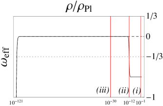
Figure 1: Evolution of the equation of state parameter for $\mu=-10^{24}$: the solid line corresponds to the effective EoS of QTG as a function of the effective energy density, Eq.(16); the dashed black line corresponds to the EH case, $\omega_{0}(\varrho_{0})$; the red lines are the entropy densities of the apparent cosmological horizon, Eq.(3), for (i) $\lambda=-9.00\times 10^{22}$ ; (ii) $\lambda=-2.50\times 10^{51}$ ; (iii) $\lambda=7.53\times 10^{69}$.

This effect may be seen in Fig.1, where $\omega_{0}(\varrho_{0})$, given by Eq.(12), is shown as the dashed line, while the continuous black line depicts the effective equation of state (16). Here $w_{1}=0$, and $w_{2}$ is fixed by the observed value of the cosmological constant (cf. Eq.(20)). One can clearly see that as the energy density increases the plot of $\omega_{\mathrm{eff}}$ sinks beneath the line of $-1/3$, indicating the new period of accelerated expansion. For smaller densities, however, there is very little difference between the EH plot and the QTG one. Although some of the indispensable features of inflation – slow-roll, for example – are not present, we shall freely nominate this early acceleration period as an “inflationary”. The duration of such a “rustic inflation” evidently depends on the value of $\mu$. By imposing $\omega_{\mathrm{eff}}(\varrho_{\mathrm{acc}})=-1/3$, we get a cubic equation:

$$\frac{(w_{1}-1)}{36}\varkappa^{4}\,\mu L^{4}\;\varrho_{\mathrm{acc}}^{3}-\frac{3w_{1}+1}{3}\varrho_{\mathrm{acc}}+w_{2}=0\;,$$ (17)

whose positive real roots give the threshold of the two acceleration periods now present in the dynamics – the initial one due to QTG and the final due to the cosmological constant. The number of distinct real solutions depends on the sign of the discriminant of (17) and, for $\mu<0$ and $w_{1}>-1/3$, it determines a critical value

$$|\mu_{{\mathrm{acc}}}|=\frac{16(3w_{1}+1)^{3}}{81(1-w_{1})\varkappa^{4}w_{2}^{2}L^{4}}$$

for which the discriminant vanishes. Thus if $|\mu|<|\mu_{{\mathrm{acc}}}|$ there are two positive real roots for (17), corresponding to two distinct periods of acceleration. But for large enough values of the gravitational coupling, namely $|\mu|\geq|\mu_{{\mathrm{acc}}}|$, there is no positive real root to (17) and as a consequence the initial QTG acceleration period lasts for such a long time that it merges with the final one – the universe is then never decelerated.

It is worthwhile to remark here that in the QTG counterpart (16) of the EH linear EoS, for $\mu<0$ the effective speed of sound $v_{\mathrm{eff}}^{2}=\partial p/\partial\varrho$ also satisfies the causality conditions $-1<v_{\mathrm{eff}}^{2}<1$, under the same restrictions on the parameters $w_{1}$ and $w_{2}$. On the other hand, for $\mu>0$, we see that $v_{\mathrm{eff}}^{2}\to\infty$ as $\varrho\to\frac{2}{L^{2}\varkappa^{2}}\sqrt{3/\mu}$. This non-causal behaviour of the effective fluid near the points where $C_{0}(\varrho)=0$ is yet another reason to consider here only the case of negative values of $\mu$.

Although the form of $t(H)$ given by Eq.(14) does not allow to analytically determine the exact form of the Hubble function $H(t)$, we may invert it in a first order approximation. This is possible when the dimensionless quantity $|\mu|L^{4}H^{4}$ is much smaller than unity. For $L=l_{\mathrm{Pl}}$, such an approximation is valid during most of the universe history, since $H(t)$ is typically of a cosmological order (greater than 1 Mpc $\sim 10^{57}\times l_{\mathrm{Pl}}$). In what follows, we shall refer to this approximation as “first order in $|\mu|$”:

$$H(t;\mu)=H_{0}(t)+\mu\,H_{1}(t)+\cdots,$$

$$a(t,\mu)=a_{0}(t)\left[1+\mu\,A_{1}(t)+\cdots\right],$$

with the scale factor parametrized as $a(t)=e^{A(t)}$. In zeroth order we have, naturally, the EH solution:

$$H_{0}(t)=\varkappa\sqrt{\frac{w_{2}}{6(1+w_{1})}}\,{\mathrm{cth}}\left[(t-t_{0})/\tau\right],$$ (18)

$$a_{0}(t)=\tilde{a}_{0}\,{\mathrm{sh}}^{\delta}\left[(t-t_{0})/\tau\right],\;\;\delta=\frac{2}{3(1+w_{1})}\;.$$ (19)

Here $1/\tau=\varkappa\sqrt{3(1+w_{1})\,w_{2}/8}$, and $\tilde{a}_{0}$ is a normalization constant. At early times $a_{0}(t)\sim\tilde{a}_{0}(t/\tau)^{\delta}$ the observed behaviour is typical of cosmologies with constant EoS: $p_{0}/\varrho_{0}\approx w_{1}$. Later, for $t/\tau\gg 1$ the cosmological constant

$$\Lambda_{0}=\varkappa^{2}w_{2}/8(1+w_{1})$$ (20)

dominates the EoS and the universe enters a final, accelerated, asymptotically de Sitter phase, with an asymptotically constant energy density $\varrho_{\Lambda_{0}}=w_{2}/(1+w_{1})$. Then

$$a_{0}(t)\sim\exp\left\{2\sqrt{\frac{\Lambda_{0}}{3}}\,(t-t_{0})\right\}\;.$$ (21)

In particular, by choosing $w_{1}=0$, and thus $\delta=2/3$, we see that (12) describes fairly well our observed Universe, neglecting inflation and the radiation dominated era: we begin at $t=0$ with a dust-filled space-time, which ends at a de Sitter space with $\Lambda_{0}$ presenting observed value [10]

$$\Lambda_{0}\approx 3.14\times 10^{-122}\times l_{\mathrm{Pl}}^{-2}\;,$$ (22)

if we choose $w_{2}$ accordingly, using Eq.(20).

The first order corrections can be easily calculated from Eq.(13):

$$H_{1}(t)=\frac{\tilde{H}_{1}}{{\mathrm{sh}}^{2}\left((t-t_{0})/\tau\right)}\Big{\{}\frac{t-t_{0}}{4\tau}-\frac{1}{8}{\mathrm{sh}}\left(\frac{2(t-t_{0})}{\tau}\right)-$$

$$-\frac{1}{3}{\mathrm{cth}}\left(\frac{t-t_{0}}{\tau}\right)\left[{\mathrm{sh}}^{-2}\left(\frac{t-t_{0}}{\tau}\right)+\frac{5}{2}\right]\Big{\}};$$ (23)

$$A_{1}(t)=\frac{\tilde{H}_{1}\tau}{12}\Big{\{}{\mathrm{cth}}\left(\frac{t}{\tau}\right)\left[5\,{\mathrm{cth}}\left(\frac{t}{\tau}\right)-\frac{3t}{\tau}\right]+{\mathrm{sh}}^{-4}\left(\frac{t}{\tau}\right)\Big{\}}\;,$$ (24)

where $\tilde{H}_{1}=-\varkappa^{6}\,w_{2}^{3}\,\tau L^{4}/72(1+w_{1})^{2}$. The constant $t_{0}=4\pi\upsilon/3(1+w_{1})\mu L^{4}$ assures that the singularity is placed in $t=0$, and as $\mu\to 0$ also $t_{0}\to 0$. From the scale factor and the Hubble function, one can determine all other relevant quantities, and in particular the effective energy density $\varrho(t)$, plotted in Fig.2.

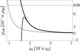
Figure 2: Time evolution of the energy density, for the same parameters of Fig.1. The black continuous curve gives the exact function $\varrho(t)$, obtained from graphical inversion of $t(\varrho)$ given by Eq.(14); the black dashed line gives the first order approximation; the dotted gray line depicts the EH density $\varrho_{0}(t)$; the horizontal gray line marks the final energy density of the early acceleration period.

As one approaches the initial singularity at $t=0$, Eq.(14) shows that $H$ diverges. Eventually we then have $H\gtrsim 1/l_{\mathrm{Pl}}$ and the first order approximation is bound to fail – indeed, $H_{1}(t)$ diverges more rapidly than $H_{0}(t)$ as $t\to 0$. This can be clearly seen in Fig.2: the black continuous line shows the exact function $\varrho(t)$, obtained from graphical inversion of $t(\varrho)$ given by Eq.(14); the black dashed line shows the first order approximation $H_{0}(t)+\mu H_{1}(t)$. It is clear that the first order approximation is only valid valid for times greater than an instant $t_{*}$, when the curve has a maximum, but for $t>t_{*}$ it is in good agreement with the exact solution. To smallest order in $|\mu|$, we have

$$t_{*}\approx\left(2(1+w_{1})^{3/8}+\pi\right)\frac{\sqrt{2}}{3(1+w_{1})}\,L|\mu|^{1/4}\;.$$ (25)

Now, approximating to first order Eq.(17) we find that the initial period ends when the effective energy density decreases to the value

$$\varrho_{\mathrm{initial}}\approx\sqrt{\frac{1+3w_{1}}{1-w_{1}}}\,l_{\mathrm{Pl}}^{-2}\;(L^{4}\,|\mu|)^{-1/2},$$ (26)

which according to Eq.(14) happens at the instant

$$t_{\mathrm{acc}}\approx\frac{(\sqrt{3}+\pi)\sqrt{2}}{3(1+w_{1})}\;L\,|\mu|^{1/4}\;.$$ (27)

This shows that $t_{*}$ is slightly posterior to $t_{\mathrm{acc}}$, hence an approximation to only first order is not sufficient to describe the initial acceleration period created by QTG.

As we have shown above, if $|\mu|\gg|\mu_{\mathrm{acc}}|$ we may have an eternally accelerated expansion. Such large values of $|\mu|$, therefore, do not correspond reasonably to the observed universe. One might thus pose the question: What are the restrictions on the values of the gravitational couplings $\lambda$ and $\mu$, which guarantee the physical consistency of the quasi-topological effects? Regarding the initial acceleration period as an inflation era, we may assume that it would occur in the range of energies $\varrho_{\mathrm{Pl}}\gtrsim\varrho\gtrsim 10^{-12}\times\varrho_{\mathrm{Pl}}$ (see [29]), thus we must have $\mu_{\mathrm{acc}}$ such that the root of (17) lies within this bound. The upper bound of this interval, viz. $\varrho_{\mathrm{acc}}\sim 10^{-12}\times\varrho_{\mathrm{Pl}}$, is indeed the case depicted in Figs.1 and 2, what serves to demonstrate the validity of the first order approximation. Another phenomenological restriction stems from the fact the the apparent horizon entropy should not be vanishing for too small values of $\varrho$. In the GB case, there is no initial acceleration period, and this entropic restriction is in fact the only condition we have on $\lambda$. It is quite evident from Eq.(10) that one may choose $\lambda$ to get $\varrho_{\mathrm{GB}}$ as large as one needs – e.g. for $\lambda=3/4$ we have $\varrho_{\mathrm{GB}}=\varrho_{\mathrm{Pl}}$. In QTG instead, as it may be easily seen from Eq.(11), for each given value of $\mu$ determining the end of the acceleration period, we can choose $\lambda$ in order to place $\varrho_{\mathrm{QTG}}$: (i) before or (iii) after $\varrho_{\mathrm{initial}}$, or even to have (ii) $\varrho_{\mathrm{QTG}}=\varrho_{\mathrm{initial}}$. This is exemplified in Fig.1, where the red lines represent the values of $\varrho$ for which $s(\varrho)=0$. Note that in cases (ii) and (iii) the whole initial acceleration period is rendered “unphysical” on account of the negative horizon entropy there.

5 On the late Universe QTG effects

Although the more significant effects of QTG take place when the curvature, as well as the energy density, are big enough – namely, at early times – it turns out that the whole evolution of the universe is modified by the QTG terms. Clearly, at later times, as the curvature diminishes, the cubic and quadratic terms in (1) become more and more negligible and the first order approximation made in the last section is then justified.

An example of such changes is given by the fact that the cosmological constant, which characterizes the geometry of the asymptotically ${\mathrm{dS}}_{4}$ spaces in the limit $t\to\infty$, is not equal to the bare one, $\Lambda_{0}$, defined by the matter Lagrangian. Indeed, in QTG one observes the effective cosmological constant $\Lambda_{\mathrm{eff}}$, related to the Hubble function $H(t)$. To first order in $\mu$, one may determine $\Lambda_{\mathrm{eff}}$ by the approximation (23) for $H(t)$, or else by inverting directly the exact equation

$$\Lambda_{0}=\Lambda_{\mathrm{eff}}\left(1-\mu L^{4}\Lambda_{\mathrm{eff}}^{2}/9\right)\;,$$ (28)

obtained from Eq.(8): $\Lambda_{\mathrm{eff}}\approx\Lambda_{0}+L^{4}\mu\,\Lambda_{0}^{3}/9\;$. This is in fact a general result, valid for every asymptotically de Sitter space, regardless of the particular matter EoS leading to the final ${\mathrm{dS}}_{4}$ vacuum. Notice that for the very small value of the observed cosmological constant, both $\Lambda_{0}$ and $\Lambda_{\mathrm{eff}}$ are practically equal.

Another feature of asymptotically de Sitter space-times is the presence of a future event horizon. Its comoving radius is given by the integral $r_{f}(t)=\int_{t}^{\infty}{\mathrm{d}}t/a(t)$ and may be calculated to first order in $\mu$ by using the results (19) and (24). At zeroth order (i.e. in the EH case) this yields

$$r^{(0)}_{f}(t)=\frac{\tau}{\delta\,\tilde{a}_{0}}\,\frac{1}{{\mathrm{ch}}^{\delta}(t/\tau)}\,{}_{2}{\mathrm{F}}_{1}\left[\frac{\delta}{2}\,,\,\left(\frac{1+\delta}{2}\right)\,;\,\frac{2+\delta}{2}\,;\,\frac{1}{{\mathrm{ch}}^{2}(t/\tau)}\right],$$ (29)

while the first order QTG correction is given by:

$$r^{(1)}_{f}(t)=\frac{\tilde{H}_{1}\tau^{2}}{12\tilde{a}_{0}}\Bigg{\{}\frac{5/\delta}{{\mathrm{ch}}^{\delta}(t/\tau)}\,{}_{2}{\mathrm{F}}_{1}\left[\frac{\delta}{2},\frac{3+\delta}{2};\frac{2+\delta}{2};\frac{1}{{\mathrm{ch}}^{2}(t/\tau)}\right]+$$

$$+\frac{1/(4+\delta)}{[{\mathrm{ch}}(t/\tau)]^{(4+\delta)}}\,{}_{2}{\mathrm{F}}_{1}\left[\frac{4+\delta}{2},\frac{5+\delta}{2};\frac{6+\delta}{2};\frac{1}{{\mathrm{ch}}^{2}(t/\tau)}\right]-\frac{3t/(\delta\tau)}{{\mathrm{sh}}^{\delta}(t/\tau)}-$$

$$-\frac{3/\delta^{2}}{{\mathrm{ch}}^{\delta}(t/\tau)}\,{}_{2}{\mathrm{F}}_{1}\left[\frac{\delta}{2},\frac{1+\delta}{2};\frac{2+\delta}{2};\frac{1}{{\mathrm{ch}}^{2}(t/\tau)}\right]\Bigg{\}}.$$ (30)

The function $r_{f}(t)$ describes the past light cone of the (infinite) future of the comoving observer at the origin. The tip of this cone is placed at $\{r_{f}=0,\,t=\infty\}$. Then as $t\to\infty$ the physical radius, $l_{f}(t)=a(t)\,r_{f}(t)$ becomes equal to the (constant) de Sitter radius $1/H$. The first order approximation to $l_{f}(t)$ can be easily obtained with the help of Eq.(24): for example its value today, at $t=13.8\;{\mathrm{Gyrs}}$, is $l_{f}\approx\left(4.90\times 10^{3}+\mu\times 9.10\times 10^{-248}\right){\mathrm{Mpc}}\;$.

Alternatively, the comoving radius $r_{p}(t)=\int^{t}_{\tilde{t}}{\mathrm{d}}t/a(t)$ describes the future light cone for an observer at the origin, starting from its tip at $\{r_{p}=0,\,t=\tilde{t}\}$. In a singular universe, if this tip is placed at the beginning of time, $\tilde{t}=0$, then $r_{p}(t)$ is the particle horizon. In practice, the choice of $\tilde{t}$ determines only a constant, for we may write

$$r_{p}(t)=-\int_{t}^{\infty}{\mathrm{d}}t/a(t)+\int_{\tilde{t}}^{\infty}{\mathrm{d}}t/a=-r_{f}(t)+r_{f}(\tilde{t})\;.$$ (31)

Thus for example, in the EH case with $\tilde{t}=0$, Eq.(29) gives

$$r^{(0)}_{p}(t)=-\frac{\tau/\delta\tilde{a}_{0}}{{\mathrm{ch}}^{\delta}(t/\tau)}\,{}_{2}{\mathrm{F}}_{1}\left[\frac{\delta}{2},\frac{1+\delta}{2};\frac{2+\delta}{2};\frac{1}{{\mathrm{ch}}^{2}(t/\tau)}\right]+\frac{\tau}{2\tilde{a}_{0}}{\mathrm{B}}\left(\frac{\delta}{2},\frac{1-\delta}{2}\right),$$ (32)

and in general Eqs.(29) and (30) determine also the first order correction for $r_{p}(t)$, for a given $\tilde{t}$.

Recall that the first order approximation for the scale factor is only valid for $t\gtrsim t_{*}$, with $t_{*}$ denoting the instant where the approximation fails, Eq.(25). Therefore in QTG we have the “technical” impossibility of placing the tip of the light cone on the initial singularity – the earlier we may place it is at $\tilde{t}=t_{*}$. Due to the fact that $t_{*}$ (at our first approximation) is slightly posterior to $t_{\mathrm{acc}}$, we are then technically prevented from describing the increase of the particle horizon during this early “inflationary” period. Consequently, we cannot determine its number of $e$-foldings, and whether it solves the usual problems of non-inflationary cosmology – such as, for example, the horizon problem.

The knowledge of the above expressions for the radii $r_{p}(t)$ and $r_{f}(t)$ provides an analytic description of the causal diamond [30, 31] and its comoving volume $V_{{\mathrm{c.d.}}}(t)$, in the QTG cosmological model under investigation. The former is defined as the intersection of the causal past of the “point” $\{r_{f}=0,\,t=\infty\}$ and the causal future of $\{r_{p}=0,\,t=\tilde{t}\}$. At each instant $t$ the volume is given by $V_{\mathrm{c.d.}}=\frac{4}{3}\pi r^{3}(t)$ with $r=r_{p}$ on the upper and $r=r_{f}$ on the lower half of it. It is easily seen that $V_{\mathrm{c.d.}}$ has a single maximum at $t=t_{\mathrm{edge}}$, when $r_{p}(t_{\mathrm{edge}})=r_{f}(t_{\mathrm{edge}})$ [31]. With the aid of Eq.(31), the instant $t_{\mathrm{edge}}$ is determined from the equation $r_{f}(t_{\mathrm{edge}})=\frac{1}{2}r_{f}(\tilde{t})$, which is exact, i.e. independent from the first order approximation. If $r_{f}(t)$ is a continuous function, then we conclude that a first order correction to $\tilde{t}$ must imply a first order change in $t_{\mathrm{edge}}$. Therefore for small $t_{*}=\tilde{t}$ in QTG, the edge of the causal diamond occurs at an instant differing not more than at first order from the corresponding value in EH.

In EH gravity with linear EoS (12) and $w_{1}=0$, describing an early universe dominated by dust, Bousso et al. [10] have calculated $V_{\mathrm{c.d.}}(t)$ and used it to predict the order of magnitude of the observed cosmological constant. Their analysis, based on the rather universal (phenomenological) evaluation of the entropy production rate in our universe, demonstrates that only when $\Lambda_{0}\sim 10^{-122}\times l_{\mathrm{Pl}}^{-2}$ the causal entropic principle (CEP), requiring maximal entropic production within the corresponding causal diamond volume, is fulfilled. According to their arguments the main production of bulk entropy occurs during the matter-dominated era. Therefore one can perform a similar analysis for the QTG extension of this linear EoS model, by imposing the $CEP$ conditions for the causal diamond whose inferior tip is placed at $\tilde{t}=t_{*}$, thus respecting the restrictions of the considered first approximation. Surely, even if the tips of the causal diamonds in QTG and in EH gravity were placed at the same point – say, by replacing $t=0$ with $t=t_{*}$ in the EH case as well –, still they would not be identical due to the changes in the dynamics given in (30). However, as we saw above, the first order QTG corrections we are considering do not change significantly the comoving volume of the causal diamond, and in fact they lead to the same prediction for the magnitude of the effective cosmological constant $\Lambda_{\mathrm{eff}}\approx\Lambda_{0}+L^{4}\mu\,\Lambda_{0}^{3}/9\;\sim 10^{-122}\times l_{\mathrm{Pl}}^{-2}$.

Throughout this discussion, we have not taken into account the entropic bounds derived in Sect.3. Regardless of our technical restrictions for placing the inferior tip of the causal diamond, in the case of $\mu<0$, we cannot place it before the instant $t_{\mathrm{QTG}}$ when the apparent horizon’s entropy vanishes. The same is true in the GB case, for $\lambda>0$. We are however assuming that $t_{\mathrm{QTG}}$ is very small, in particular that $t_{\mathrm{QTG}}\lesssim t_{*}$. This can always be set for an appropriate value of $\lambda$. Either way, the entropic restrictions do not allow the inferior tip of the causal diamond to be placed on the singularity.

Let us list in conclusion a few open problems concerning the considered (linear EoS) cosmological model of the cubic Quasi-Topological gravity: (a) The stability conditions for the asymptotic ${\mathrm{dS}}_{4}$ cosmological QTG solutions, which requires the calculation of the spectrum of the corresponding linear fluctuations at least in the probe approximation; (b) The analysis of the properties of QTG models with more realistic matter content by considering EoS or equivalently (string inspired) matter superpotentials [32] giving rise to early-time inflation with a desired slow-roll behaviour, which is under investigation [14]. It is worthwhile to also mention that the methods and some of the results of the present paper seem to have a straightforward “cosmological” application to the recently constructed “higher curvature” quartic QTG extension [33] of the EH gravity, as well as to the case of spatially curved FRW solutions of the considered four dimensional, cubic QTG model.

Acknowledgments. We are grateful to C.P. Constantinidis for his collaboration in the initial stage of this work and for the discussions.

References

- [1] N.D. Birrell and P.C.W. Davies, Quantum fields in curved space, Cambridge University Press, Cambridge, 1984.
- [2] G. ’t Hooft and M.J.G. Veltman, One loop divergencies in the theory of gravitation, Annales Poincare Phys. Theor. A 20 (1974) 69.
- [3] K.S. Stelle, Renormalization of Higher Derivative Quantum Gravity, Phys. Rev. D 16 (1977) 953.
- [4] S.’i. Nojiri and S.D. Odintsov, Unified cosmic history in modified gravity: from F(R) theory to Lorentz non-invariant models, Phys. Rept. 505 (2011) 59 [arXiv:1011.0544 [gr-qc]].
- [5] S. Capozziello and M. De Laurentis, Extended Theories of Gravity, Phys. Rept. 509 (2011) 167 [arXiv:1108.6266 [gr-qc]].
- [6] T. Clifton, P.G. Ferreira, A. Padilla and C. Skordis, Modified Gravity and Cosmology, Phys. Rept. 513 (2012) 1 [arXiv:1106.2476 [astro-ph.CO]].
- [7] J. Oliva and S. Ray, Classification of Six Derivative Lagrangians of Gravity and Static Spherically Symmetric Solutions, Phys. Rev. D 82 (2010) 124030 [arXiv:1004.0737 [gr-qc]].
- [8] U. Camara da Silva, C.P. Constantinidis, A.L. Alves Lima and G.M. Sotkov, Domain Walls in Extended Lovelock Gravity, JHEP 1204 (2012) 109 [arXiv:1202.4682 [hep-th]].
- [9] A. Sinha, On higher derivative gravity, -theorems and cosmology, Class. Quant. Grav. 28 (2011) 085002 [arXiv:1008.4315 [hep-th]].
- [10] R. Bousso, R. Harnik, G.D. Kribs and G. Perez, Predicting the Cosmological Constant from the Causal Entropic Principle, Phys. Rev. D 76 (2007) 043513 [hep-th/0702115 [HEP-TH]].
- [11] P.-H. Chavanis, Models of universe with a polytropic equation of state: II. The late universe, arXiv:1208.0801 [astro-ph.CO].
- [12] N. Kaloper and A.D. Linde, Cosmology versus holography, Phys. Rev. D 60 (1999) 103509 [hep-th/9904120].
- [13] E. Babichev, V. Dokuchaev and Y. Eroshenko, Dark energy cosmology with generalized linear equation of state, Class. Quant. Grav. 22 (2005) 143 [astro-ph/0407190].
- [14] U. Camara dS, C.P. Constantinidis, A.L. Lima, G.M. Sotkov, Inflaton superpotential for extended cubic Lovelock Gravity, in preparation.
- [15] J.M. Bardeen, B. Carter and S.W. Hawking, The Four laws of black hole mechanics, Commun. Math. Phys. 31 (1973) 161.
- [16] S.W. Hawking, Particle Creation by Black Holes, Commun. Math. Phys. 43 (1975) 199 [Erratum-ibid. 46 (1976) 206].
- [17] G.W. Gibbons and S.W. Hawking, Cosmological Event Horizons, Thermodynamics, and Particle Creation, Phys. Rev. D 15 (1977) 2738.
- [18] T. Jacobson, “Thermodynamics of space-time: The Einstein equation of state,” Phys. Rev. Lett. 75 (1995) 1260 [gr-qc/9504004].
- [19] R. Guedens, T. Jacobson and S. Sarkar, Horizon entropy and higher curvature equations of state, Phys. Rev. D 85 (2012) 064017 [arXiv:1112.6215 [gr-qc]].
- [20] T. Padmanabhan, Thermodynamical Aspects of Gravity: New insights, Rept. Prog. Phys. 73 (2010) 046901 [arXiv:0911.5004 [gr-qc]].
- [21] R.-G. Cai and S.P. Kim, First law of thermodynamics and Friedmann equations of Friedmann-Robertson-Walker universe, JHEP 0502 (2005) 050 [hep-th/0501055].
- [22] M. Akbar and R.-G. Cai, Thermodynamic Behavior of Friedmann Equations at Apparent Horizon of FRW Universe, Phys. Rev. D 75 (2007) 084003 [hep-th/0609128].
- [23] R.M. Wald, Black hole entropy is the Noether charge, Phys. Rev. D 48 (1993) 3427 [gr-qc/9307038].
- [24] V. Iyer and R.M. Wald, Some properties of Noether charge and a proposal for dynamical black hole entropy, Phys. Rev. D 50 (1994) 846 [gr-qc/9403028].
- [25] S.A. Hayward, Unified first law of black hole dynamics and relativistic thermodynamics, Class. Quant. Grav. 15 (1998) 3147 [gr-qc/9710089].
- [26] U. Camara dS, A.A. Lima, and G.M. Sotkov, Modified Friedmann Equations from the First Law of Thermodynamics in Quasi-Topological Cosmology, in preparation.
- [27] S. Capozziello, S. Nojiri and S.D. Odintsov, Dark energy: The Equation of state description versus scalar-tensor or modified gravity, Phys. Lett. B 634 (2006) 93 [hep-th/0512118].
- [28] S.Capozziello, V.F. Cardone, E. Elizalde, S. Nojiri and S.D. Odintsov, Observational constraints on dark energy with generalized equations of state, Phys. Rev. D 73 (2006) 043512 [astro-ph/0508350].
- [29] A.D. Linde, Inflationary Cosmology, Lect. Notes Phys. 738 (2008) 1 [arXiv:0705.0164 [hep-th]].
- [30] G.W. Gibbons and S.N. Solodukhin, The Geometry of Large Causal Diamonds and the No Hair Property of Asymptotically de-Sitter Spacetimes, Phys. Lett. B 652 (2007) 103 [arXiv:0706.0603 [hep-th]].
- [31] R. Bousso, Positive vacuum energy and the N bound, JHEP 0011 (2000) 038 [hep-th/0010252].
- [32] S. Kachru, R. Kallosh, A.D. Linde and S.P. Trivedi, De Sitter vacua in string theory, Phys. Rev. D 68 (2003) 046005 [hep-th/0301240].
- [33] M.H. Dehghani, A. Bazrafshan, R.B. Mann, M.R. Mehdizadeh, M. Ghanaatian and M.H. Vahidinia, Black Holes in Quartic Quasitopological Gravity, Phys. Rev. D 85 (2012) 104009 [arXiv:1109.4708 [hep-th]].