Multi-reference symmetry-projected variational approaches for ground and excited states of the one-dimensional Hubbard model

Abstract

We present a multi-reference configuration mixing scheme for describing ground and excited states, with well defined spin and space group symmetry quantum numbers, of the one-dimensional Hubbard model with nearest-neighbor hopping and periodic boundary conditions. Within this scheme, each state is expanded in terms of non-orthogonal and variationally determined symmetry-projected configurations. The results for lattices up to 30 and 50 sites compare well with the exact Lieb-Wu solutions as well as with results from other state-of-the-art approximations. In addition to spin-spin correlation functions in real space and magnetic structure factors, we present results for spectral functions and density of states computed with an ansatz whose quality can be well-controlled by the number of symmetry-projected configurations used to approximate the systems with $N_{e}$ and $N_{e}\pm 1$ electrons. The intrinsic symmetry-broken determinants resulting from the variational calculations have rich structures in terms of defects that can be regarded as basic units of quantum fluctuations. Given the quality of the results here reported, as well as the parallelization properties of the considered scheme, we believe that symmetry-projection techniques, which have found ample applications in nuclear structure physics, deserve further attention in the study of low-dimensional correlated many-electron systems.

I Introduction.

Studies of correlations arising from electron-electron interactions remain a central theme in condensed matter physis Dagotto-review to better understand challenging phenomena such as high-Tc superconductivity HTCSC-1 or colossal magnetic resistance. Science-Dagotto There is a need for better theoretical models that can account for relevant correlations in ground and excites states of fermionic systems with as much simplicity as possible. Within this context, the repulsive Hubbard Hamiltonian Hubbard-model_def1 has received a lot of attention since it is considered the generic model of strongly correlated electron systems. Dagotto-review Hubbard-like models have also received renewed attention in the study of cold fermionic atoms in optical lattices optical-1 and the electronic properties of graphene. CastroNeto-review

Unlike the one-dimensional (1D) Hubbard model, which is exactly solvable LIEB using the Bethe ansatz, BETHE an exact solution of the two-dimensional (2D) problem is not known. Therefore, it is highly desirable to develop approximations that, on the one hand, can capture the main features of the exact 1D Bethe solution and, on the other hand, can be extended to higher dimensions. For small lattices, one can resort to exact diagonalization using the Lanczos method. Dagotto-review ; Lanczos-Fano For larger systems, several other methods have been extensively used to study the 1D and 2D Hubbard models as well as their strong coupling versions. text-Hubbard-1D Among such approximations, we have the quantum Monte Carlo, Nightingale ; Raedt-MC the variational Monte Carlo, Neuscamman-2012 the density matrix renormalization group DMRG-White ; Dukelsky-Pittel-RPP ; Scholl-RMP ; Xiang as well as approximations based on matrix product and tensor network states. TNPS-1 Both the dynamical mean field theory and its cluster extensions Zgid ; DMFT-1 ; maier2005 ; stanescu2006 ; moukouri2001 ; huscroft2001 ; aryanpour2003 ; DVP-2 have made important contributions to our present knowledge of the Hubbard model. Other embedding approaches are also available. Knizia-Chan Finally, we refer the reader to the recent state-of-the-art applications of the coupled cluster method to frustrated Hubbard-like models. Bishop-1 ; Bishop-2

Although routinely used in nuclear structure physics, especially within the Generator Coordinate Method, rayner-GCM-paper ; rayner-GCM-parity symmetry restoration via projection techniques rs has received little attention in condensed matter physics. Nevertheless, these techniques offer an alternative for obtaining accurate correlated wave functions that respect the symmetries of the considered many-fermion problem. The key idea is,rs on the one hand, to consider a mean-field trial state $|{\mathcal{D}}\rangle$ which deliberately breaks several symmetries of the original Hamiltonian. On the other hand, the Goldstone manifold $\hat{R}|{\mathcal{D}}\rangle$, where $\hat{R}$ represents a symmetry operation, is degenerate and the superposition of such Goldstone states, rs can be used to recover the desired symmetry by means of a self-consistent variation-after-projection procedure. rs ; Rayner-Carlo-CM-1 Such a single-reference (SR) scheme provides the optimal Ritz-variationalBlaizot-Ripka representation of a given state by means of only one symmetry-projected mean-field configuration. This kind of SR variation-after-projection scheme, has already been applied to the 1D and 2D Hubbard models Carlos-Hubbard-1D ; Rayner-2D-Hubbard-PRB-2012 as well as in quantum chemistry within the framework of the Projected Quasiparticle Theory. PQT-reference-1 ; PQT-reference-2 ; PQT-reference-3

One of the main advantages of the symmetry-projected approximations rs ; Carlos-Hubbard-1D ; Rayner-2D-Hubbard-PRB-2012 ; PQT-reference-1 ; PQT-reference-2 ; PQT-reference-3 is that they offer compact wave functions as well as a systematic way to improve their quality by adopting a multi-reference (MR) approach. In this case, a set of symmetry-broken mean-field states $|{\mathcal{D}}^{i}\rangle$ is used to build Goldstone manifolds $\hat{R}|{\mathcal{D}}^{i}\rangle$ whose superposition can be used to recover the desired symmetries of the Hamiltonian. Carlo-review ; Fukutome-original-RSHF The key idea is then to expand a given state in terms of several symmetry-projected and variationally determined mean-field configurations. The resulting wave functions encode more correlations than the ones obtained within SR methods while still keeping well defined symmetry quantum numbers. Tomita-1

There are differents flavors of MR approximations available in the literature.Carlo-review ; Fukutome-original-RSHF ; Tomita-1 ; Yamamoto-1 ; Yamamoto-2 ; Ikawa-1993 ; Tomita-2 ; Tomita-3 ; Mizusaki-1 ; Mizusaki-2 In the present study, we adopt a MR scheme well known in nuclear structure physics, Carlo-review which to the best of our knowledge has not been applied to lattice models. The key ingredient in such MR scheme is the inclusion of relevant correlations in both ground and excited states on an equal footing. As a benchmark test, we concentrate on the 1D Hubbard model for which exact solutions are known. LIEB ; BETHE In particular, we consider the case of half-filled lattices. Nevertheless, the present MR approximation can be extended to the 2D case as well as to doped systems with arbitrary on-site interaction strengths.

For a given single-electron space we resort to generalized HF-transformations StuberPaldus (GHF) mixing all quantum numbers of the single-electron basis states. The corresponding Slater determinants deliberately break spin and spatial symmetries of the 1D Hubbard Hamiltonian. text-Hubbard-1D We restore these broken symmetries with the help of projection operators. rs The resulting MR ground state wave functions are obtained applying the variational principle to the projected energy.

The structure of our MR ground state wave functions is formally similar to the one adopted within the Resonating HF Fukutome-original-RSHF ; Yamamoto-1 ; Yamamoto-2 ; Ikawa-1993 ; Tomita-1 ; Tomita-2 (ResHF) method, i.e., they are expanded in terms of a given number of non-orthogonal symmetry-projected configurations. Nevertheless, while in the latter all the underlying HF-transformations and mixing coefficients are optimized simultaneously, Tomita-1 ; Tomita-2 in our case the orbital optimization is performed sequentially, only for the last added HF-transformation (all our mixing coefficients are still optimized at the same time) rendering our calculations easier to handle. This is particularly relevant for alleviating our numerical effort if one keeps in mind that, for both ground and excited states, we use the most general GHF-transformations and therefore a full 3D spin projection is required.

Our MR scheme is also used to compute spin-spin correlation functions (SSCFs) in real space, magnetic structure factors (MSFs) as well as dynamical properties of the 1D Hubbard model like spectral functions (SFs) and density of states (DOS). Dagotto-review ; Rayner-2D-Hubbard-PRB-2012 ; Carlos-Hubbard-1D ; Fetter-W On the other hand, one may wonder whether there is any relevant information in the intrinsic symmetry-broken GHF-determinants associated with our MR wave functions. As will be shown below, the structure of such intrinsic determinants can be interpreted in terms of basic units of quantum fluctuations for the lattices considered.Horovitz

In addition to ground state properties, our MR framework treats excited states with well defined quantum numbers as expansions in terms of non-orthogonal symmetry-projected configurations using chains of variation-after-projection (VAP) calculations. As a byproduct, we also obtain a (truncated) basis consisting of a few Gram-Schmidt orthonormalized states, Rayner-2D-Hubbard-PRB-2012 which may be used to perform a final diagonalization of the Hamiltonian in order to account for further correlations in both ground and excited states.

The layout of the theory part of this paper is as follows. First, we introduce the methodology of our MR VAP scheme in Sec.II. Symmetry restoration based on a single Slater determinant (i.e., SR symmetry restoration) is described in Sec.II.1. This section will serve to set our notation as well as to introduce some key elements of our 3D spin and full space group projection techniques. Subsequently, symmetry restoration based on several Slater determinants (i.e., MR symmetry restoration) is discussed in Sec.II.2. In particular, the MR description of ground and excited states is presented in Secs.II.2.1 and II.2.2, respectively. In Sec.II.3, we will briefly discuss the computation of the SFs and DOS within our theoretical framework.

The results presented in this paper test the performance of our approximation in a selected set of illustrative examples. In most cases, calculations have been carried out for on-site repulsions $U=2t,4t$ and $8t$ taken as representatives of weak, intermediate-to-strong, and strong correlation regimes. In Sec.III, we first consider the ground states of half-filled lattices with up to 50 sites. We compare our ground state and correlation energies with the exact ones as well as with those obtained using other theoretical methods. We then discuss the dependence of the predicted correlation energies on the number of non-orthogonal symmetry-projected configurations used to expand our ground state wave functions, the computational performance of our scheme as well as the structure of the intrinsic GHF-determinants resulting from our MR VAP procedure. Next, we consider the results of our calculations for SSCFs in real space and MSFs for half-filled lattices with up to 30 sites. These results are compared with density matrix renormalization group DMRG-White ; Dukelsky-Pittel-RPP ; Scholl-RMP ; Xiang (DMRG) ones obtained with the open source ALPS software.ALPS This comparison is very valuable as DMRG represents one of the most accurate approximations in the 1D case. Subsequently, we compare the DOS provided by our theoretical framework with the exact one, obtained with an in-house diagonalization code, in a lattice with 10 sites. Results for hole SFs are also discussed for a 30-site lattice. We end Sec.III by presenting results for excitation spectra in various lattices and discussing the structure of the intrinsic GHF-determinants resulting from our MR VAP procedure for excited states. Finally, Sec.IV is devoted to concluding remarks and work perspectives.

Table 1: Ground state energy of the half-filled lattices with $N_{sites}=12$ and $20$, as predicted with the GHF-FED scheme based on $n_{1}=10$ GHF-transformations, are compared with exact results for on-site repulsions of $U=2t,4t$ and $8t$. Energies obtained with the RHF and UHF approximations are included as a reference. The ratio of correlation energies $\kappa$ obtained with the UHF and GHF-FED aproximations, is computed according to Eq.(27). For more details, see the main text.

		$N_{sites}=12$		$\kappa(\%)$		$N_{sites}=20$		$\kappa(\%)$
U=2t	RHF	-8.9282				-15.2551
	UHF	-9.3379		36.79		-15.6411		24.05
	GHF-FED	-10.0401		99.85		-16.8565		99.79
	EXACT	-10.0418				-16.8599
U=4t	RHF	-2.9282				-5.2550
	UHF	-5.6290		67.65		-9.3821		66.08
	GHF-FED	-6.9201		99.99		-11.4954		99.92
	EXACT	-6.9204				-11.5005
U=8t	RHF	9.0718				14.7450
	UHF	-2.9532		92.26		-4.9219		92.23
	GHF-FED	-3.9625		99.99		-6.5612		99.96
	EXACT	-3.9626				-6.5699

II Theoretical Framework

In what follows, we describe the theoretical framework used in the present study. First, SR symmetry restoration is presented in Sec.II.1. Subsequently, in Sec.II.2, we consider our MR scheme to describe both ground (Sec.II.2.1) and excited (Sec.II.2.2) states of the 1D Hubbard model. The computation of SFs and DOS is briefly discussed in Sec.II.3.

II.1 Single-reference (SR) symmetry restoration

We consider the 1D Hubbard Hamiltonian Hubbard-model_def1

$$\hat{H}=-t\sum_{j,\sigma}\Big{\{}\hat{c}_{j+1\sigma}^{\dagger}\hat{c}_{j\sigma}+\hat{c}_{j\sigma}^{\dagger}\hat{c}_{j+1\sigma}\Big{\}}+U\sum_{j}\hat{n}_{j\uparrow}\hat{n}_{j\downarrow}$$ (1)

where the first term represents the nearest-neighbor hopping ($t>0$) and the second is the repulsive on-site interaction ($U>0$). The fermionic Blaizot-Ripka operators $\hat{c}_{j\sigma}^{\dagger}$ and $\hat{c}_{j\sigma}$ create and destroy an electron with spin-projection $\sigma=\pm 1/2$ (also denoted as $\sigma=\uparrow,\downarrow$) along an arbitrary chosen quantization axis on a lattice site $j=1,\dots,N_{sites}$. The operators $\hat{n}_{j\sigma}=\hat{c}_{j\sigma}^{\dagger}\hat{c}_{j\sigma}$ are the local number operators. We assume periodic boundary conditions, i.e., the sites $j$ and $j+N_{sites}$ are identical. Furthermore, we assume a lattice spacing $\Delta=1$.

In the standard HF-approximation, Blaizot-Ripka ; rs the ground state of an $N_{e}$-electron system is represented by a Slater determinant $|{\mathcal{D}}\rangle=\prod_{h=1}^{N_{e}}\hat{b}_{h}^{+}|0\rangle$ in which the energetically lowest $N_{e}$ single-fermion states (holes $h,h^{{}^{\prime}},\dots$) are occupied while the remaining $2N_{sites}-N_{e}$ states (particles $p,p^{{}^{\prime}},\dots$) are empty. For a set of single-fermion operators $\hat{c}^{\dagger}$, the HF-quasiparticle operators $\hat{b}^{\dagger}$ are given by the following canonical transformation Blaizot-Ripka ; rs

$$\hat{b}_{i}^{\dagger}=\sum_{j\sigma}{\mathcal{D}}_{j\sigma,i}^{\ast}\hat{c}_{j\sigma}^{\dagger}$$ (2)

where ${\mathcal{D}}$ is a general $2N_{sites}\times 2N_{sites}$ unitary non-unitary-paper-Carlos matrix, i.e., ${\mathcal{D}}{\mathcal{D}}^{\dagger}={\mathcal{D}}^{\dagger}{\mathcal{D}}=1$. In all the calculations to be discussed below, we have used generalized HF (GHF) transformations. StuberPaldus As it is well known, the most general GHF-determinant $|{\mathcal{D}}\rangle$ deliberately breaks several symmetries of the original Hamiltonian. Carlo-review ; rs ; Rayner-2D-Hubbard-PRB-2012 ; Carlos-Hubbard-1D ; PQT-reference-1 ; PQT-reference-2 Typical examples are the rotational (in spin space) and spatial symmetries. To restore the spin quantum numbers in a symmetry-broken GHF-determinant, we explicitly use the full 3D projection operator Rayner-2D-Hubbard-PRB-2012 ; Carlos-Hubbard-1D ; PQT-reference-1 ; PQT-reference-2

$$\hat{P}_{\Sigma{\Sigma}^{{}^{\prime}}}^{S}=\frac{2S+1}{8{\pi}^{2}}\int d\Omega{\mathcal{D}}_{\Sigma{\Sigma}^{{}^{\prime}}}^{S\ast}(\Omega)R(\Omega)$$ (3)

where $R(\Omega)=e^{-i\alpha\hat{S}_{z}}e^{-i\beta\hat{S}_{y}}e^{-i\gamma\hat{S}_{z}}$ is the rotation operator in spin space, the label $\Omega=\left(\alpha,\beta,\gamma\right)$ stands for the set of Euler angles and ${\mathcal{D}}_{\Sigma{\Sigma}^{{}^{\prime}}}^{S}(\Omega)$ are Wigner functions. Edmonds To recover the spatial symmetries, we introduce the projection operator

$$\hat{P}_{mm^{{}^{\prime}}}^{k}=\frac{1}{2N_{sites}}\sum_{g}{\Gamma}_{mm^{{}^{\prime}}}^{k}(g)\hat{R}(g)$$ (4)

where ${\Gamma}_{mm^{{}^{\prime}}}^{k}(g)$ is the matrix representation of an irreducible representation, which can be found by standard methods, Tomita-1 ; Lanczos-Fano and $\hat{R}(g)$ represents the corresponding symmetry operations (i.e., translation by one lattice site and the reflection $x\rightarrow-x$) parametrized in terms of the label $g$. The linear momentum ${k}=(2\pi/N_{sites})\,{\xi}$ is given in terms of the quantum number $\xi$ that takes the values

Table 2: Ground state energy of the half-filled lattices with $N_{sites}=30$ and $50$ predicted with the GHF-FED scheme based on $n_{1}=25$ GHF-transformations, are compared with exact results for on-site repulsions of $U=2t,4t$ and $8t$. Results obtained with the UHF-ResHF approximation, Tomita-1 based on $n_{1}=30$ UHF-transformations, as well as the RHF and UHF energies are also included in the table. The ratio of correlation energies $\kappa$ obtained with the UHF, UHF-ResHF and the GHF-FED aproximations, is computed according to Eq.(27).

		$N_{sites}=30$		$\kappa(\%)$		$N_{sites}=50$		$\kappa(\%)$
U=2t	RHF	-23.2671				-38.7039
	UHF	-23.4792		10.02		-39.1294		12.02
	UHF-ResHF	-25.3436		98.11		-41.9535		91.78
	UHF-FED	-25.3508		98.45		-41.9963		92.99
	GHF-FED	-25.3730		99.50		-42.1219		96.46
	EXACT	-25.3835				-42.2443
U=4t	RHF	-8.2671				-13.7039
	UHF	-14.0732		64.75		-23.4553		65.02
	UHF-ResHF	-17.0542		98.00		-27.9633		95.09
	UHF-FED	-16.9420		96.75		-27.3518		91.01
	GHF-FED	-17.1789		99.39		-27.9788		95.19
	EXACT	-17.2335				-28.6993
U=8t	RHF	21.7329				36.2961
	UHF	-7.8329		93.65		-12.3048		92.26
	UHF-ResHF	-9.5378		99.04		-15.6422		98.59
	UHF-FED	-9.3524		98.46		-14.8461		97.08
	GHF-FED	-9.7612		99.75		-15.6753		98.65
	EXACT	-9.8387				-16.3842

$${\xi}=-\frac{N_{sites}}{2}+1,\dots,\frac{N_{sites}}{2}$$ (5)

allowed inside the Brillouin zone (BZ). Ashcroft-Mermin-book Equivalently, it can take all integer values between 0 and $N_{sites}-1$. For $k=0,\pi$ an additional label $b=\pm 1$ should be introduced to account for the parity of the corresponding irreducible representation under the reflection $x\rightarrow-x$. Tomita-1 ; Lanczos-Fano In what follows, we do not explictly write this label $b$ but the reader should keep in mind that it is taken into account whenever needed.

We introduce Rayner-2D-Hubbard-PRB-2012 the shorthand notation $\Theta=(S,k)$ for the set of symmetry (i.e., spin and linear momentum) quantum numbers as well as $K=(\Sigma,m)$. The total projection operator reads

$$\hat{P}_{KK^{{}^{\prime}}}^{\Theta}\equiv\hat{P}_{\Sigma{\Sigma}^{{}^{\prime}}}^{S}\hat{P}_{mm^{{}^{\prime}}}^{k}$$ (6)

We then superpose the Goldstone manifold $\hat{R}(\Omega)\hat{R}(g)|{\mathcal{D}}\rangle$ to recover the spin and spatial symmetries rs via the following SR ansatz

$$|{\mathcal{D}};\Theta;K\rangle=\sum_{K^{{}^{\prime}}}f_{K^{{}^{\prime}}}^{\Theta}\hat{P}_{KK^{{}^{\prime}}}^{\Theta}|{\mathcal{D}}\rangle$$ (7)

where $f^{\Theta}$ are variational parameters. Note, that the state Eq.(7) is already multi-determinantal Rayner-2D-Hubbard-PRB-2012 ; PQT-reference-1 via the projection operator $\hat{P}_{KK^{{}^{\prime}}}^{\Theta}$. For a given symmetry $\Theta$, the energy (independent of K) associated with the state Eq.(7)

$$E^{\Theta}=\frac{f^{\Theta\dagger}{\mathcal{H}}^{\Theta}f^{\Theta}}{f^{\Theta\dagger}{\mathcal{N}}^{\Theta}f^{\Theta}}$$ (8)

is given in terms of the Hamiltonian and norm

$${\mathcal{H}}_{KK^{{}^{\prime}}}^{\Theta} = \langle{\mathcal{D}}|\hat{H}\hat{P}_{KK^{{}^{\prime}}}^{\Theta}|{\mathcal{D}}\rangle$$

$${\mathcal{N}}_{KK^{{}^{\prime}}}^{\Theta} = \langle{\mathcal{D}}|\hat{P}_{KK^{{}^{\prime}}}^{\Theta}|{\mathcal{D}}\rangle$$ (9)

matrices. It has to be minimized with respect to the coefficients $f^{\Theta}$ and the underlying GHF-transformation ${\mathcal{D}}$. The variation with respect to the former yields the following resonon-like Gutzwiller_method eigenvalue equation Rayner-2D-Hubbard-PRB-2012 ; Carlos-Hubbard-1D

$$\left({\mathcal{H}}^{\Theta}-E^{\Theta}{\mathcal{N}}^{\Theta}\right)f^{\Theta}=0$$ (10)

with the constraint $f^{\Theta\dagger}{\mathcal{N}}^{\Theta}f^{\Theta}=1$ ensuring the orthogonality of the solutions. On the other hand, the unrestricted minimization of the energy [Eq.(8)] with respect to ${\mathcal{D}}$ is carried out via the Thouless theorem. Rayner-2D-Hubbard-PRB-2012 ; Carlos-Hubbard-1D ; non-unitary-paper-Carlos

For a given symmetry $\Theta$, we only retain the energetically lowest solution of our VAP equations. Rayner-2D-Hubbard-PRB-2012 Both the GHF-transformation ${\mathcal{D}}$ and the mixing coefficients $f^{\Theta}$ are complex, therefore one needs to minimize $n_{var}=2(2N_{sites}-N_{e})\times N_{e}+4S$ real variables. We use a limited-memory quasi-Newton method for such minimization. Rayner-2D-Hubbard-PRB-2012 ; Carlos-Hubbard-1D ; quasi-Newton-3 In practice, the integration over the set of Euler angles in Eq.(3) is discretized. For example, for a lattice with $N_{sites}=30$ we have used 13, 26, and 13 grid points for the integrations over $\alpha$, $\beta$, and $\gamma$, respectively. In this case, a total of 263,640 grid points are used in the discretization of the projection operator of Eq.(6). We have afforded such a task by developing a parallel implementation for all the VAP schemes discussed in this paper.

II.2 Multi-reference (MR) symmetry restoration

For each symmetry $\Theta$, the SR procedure described in Sec.II.1 provides us with the optimal variational representation of the corresponding ground state via a single symmetry-projected GHF-determinant. However, as the lattice size increases one may adopt a MR perspective to keep and/or improve the quality of the wave functions. Carlo-review ; Fukutome-original-RSHF The key features of our MR approach, known in nuclear structure physics as the FED VAMP Carlo-review (Few Determinant Variation After Mean-field Projection) strategy, for the considered ground states are described in the next subsection. We use the acronym GHF-FED to refer to it in the present work. On the other hand, our MR approach for excited states, known as EXCITED FED VAMP, Carlo-review will be presented in Sec.II.2.2. We will use the acronym GHF-EXC-FED to refer to it in what follows.

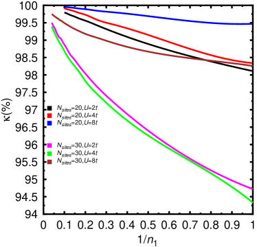
Figure 1: (Color online) The ratio of correlation energies $\kappa$ obtained with the GHF-FED approximation is plotted as a function of the inverse of the number of GHF-transformations for the half-filled lattices with $N_{sites}=20$ and $30$. Results are shown for on-site repulsions of $U=2t,4t$ and $8t$. For more details, see the main text.

II.2.1 MR symmetry restoration for ground states (GHF-FED)

Our goal in this section is to obtain, through a chain of VAP calculations, non-orthogonal symmetry-projected GHF-configurations used to build a MR expansion of a given ground state Carlo-review with well defined symmetry quantum numbers $\Theta$.

Suppose we have generated a ground state solution $|\phi_{1K}^{1\Theta}\rangle=|{\mathcal{D}}_{1}^{1};\Theta;K\rangle$ [Eq.(7)]. Note that at this point, we have added the superscript $1$ to explicitly indicate that only one GHF-transformation has been used within the SR approximation discussed in Sec.II.1. On the other hand, the subscript $1$ has been added to indicate that the ground state is considered. As we will see in Sec.II.2.2, this subscript will allow us to distinguish between ground (i.e., $i=1$) and excited (i.e., $i=2,3,\dots,m$) states. On the other hand, both indices are also added to the (intrinsic) GHF-transformation to explicitly indicate that it is variationally optimized for the state $|\phi_{1K}^{1\Theta}\rangle$. We then keep the transformation ${\mathcal{D}}_{1}^{1}$ fixed and consider the ansatz

$$|\phi_{1K}^{2\Theta}\rangle=\sum_{K^{{}^{\prime}}}\sum_{i=1}^{2}f_{1K^{{}^{\prime}}}^{i\Theta}\hat{P}_{KK^{{}^{\prime}}}^{\Theta}|{\mathcal{D}}_{1}^{i}\rangle$$ (11)

which approximates the ground state (subscript 1) by means of two (superscript 2) non-orthogonal symmetry-projected GHF-determinants. It is obtained applying the variational principle to the energy functional with respect to the last added transformation ${\mathcal{D}}_{1}^{2}$ and all the new mixing coefficients $f_{1}^{i\Theta}$. A similar procedure can be followed to approximate the ground state by a larger number of non-orthogonal symmetry-projected configurations. Let us assume that $n_{1}-1$ configurations have already been computed. Then, one introduces a new GHF-transformation ${\mathcal{D}}_{1}^{n_{1}}$, a new set of mixing coefficients $f_{1}^{i\Theta},$ and makes the MR GHF-FED ansatz

$$|\phi_{1K}^{n_{1}\Theta}\rangle=\sum_{K^{{}^{\prime}}}\sum_{i=1}^{n_{1}}f_{1K^{{}^{\prime}}}^{i\Theta}\hat{P}_{KK^{{}^{\prime}}}^{\Theta}|{\mathcal{D}}_{1}^{i}\rangle$$ (12)

which superposes the Goldstone manifolds $\hat{R}(\Omega)\hat{R}(g)|{\mathcal{D}}_{1}^{i}\rangle$. The corresponding energy

$$E_{1}^{n_{1}\Theta}=\frac{f^{n_{1}\Theta\dagger}{\mathcal{H}}^{n_{1}\Theta}f^{n_{1}\Theta}}{f^{n_{1}\Theta\dagger}{\mathcal{N}}^{n_{1}\Theta}f^{n_{1}\Theta}}$$ (13)

is given in terms of the Hamiltonian and norm

$${\mathcal{H}}_{iK,jK^{{}^{\prime}}}^{n_{1}\Theta} = \langle{\mathcal{D}}_{1}^{i}|\hat{H}\hat{P}_{KK^{{}^{\prime}}}^{\Theta}|{\mathcal{D}}_{1}^{j}\rangle$$

$${\mathcal{N}}_{iK,jK^{{}^{\prime}}}^{n_{1}\Theta} = \langle{\mathcal{D}}_{1}^{i}|\hat{P}_{KK^{{}^{\prime}}}^{\Theta}|{\mathcal{D}}_{1}^{j}\rangle$$ (14)

kernels, which require the knowledge of the symmetry-projected matrix elements between all the GHF-determinants used in the expansion Eq.(12). The wave function Eq.(12) is determined varying the energy Eq.(13) with respect to all the new mixing coefficients $f_{1}^{i\Theta}$ and the last added transformation ${\mathcal{D}}_{1}^{n_{1}}$. In the former case, we obtain an eigenvalue equation similar to Eq.(10), with the constraint $f^{n_{1}\Theta\dagger}{\mathcal{N}}^{n_{1}\Theta}f^{n_{1}\Theta}=1$, while the unrestricted minimization with respect to ${\mathcal{D}}_{1}^{n_{1}}$ is carried out via the Thouless theorem. Let us stress that the GHF-FED MR approximation Eq.(12) of a given ground state enlarges the flexibity in our wave functions to a total number of $n_{var}=2n_{1}(2N_{sites}-N_{e})\times N_{e}+4n_{1}S+2(n_{1}-1)$ variational parameters.

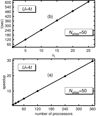
Figure 2: Speedup of a typical GHF-FED calculation is shown in panel (a) as a function of the number of proccessors. The corresponding scaling (for a fixed number of proccessors) with the number of transformations $n_{1}$ is presented in panel (b). Results are for the half-filled lattice with $N_{sites}=50$ and $U=4t.$

II.2.2 MR symmetry restoration for excited states (GHF-EXC-FED)

In this section, we construct non-orthogonal symmetry-projected GHF-configurations to expand a given excited state. The orthogonalization between ground and excited states is achieved via the Gram-Schmidt procedure. Rayner-2D-Hubbard-PRB-2012 As a byproduct, our MR GHF-EXC-FED method also yields a (truncated) basis consisting of a few orthonormal states which may be used to diagonalize the Hamiltonian and account for further correlations in both ground and excited states. Rayner-2D-Hubbard-PRB-2012 ; Carlo-review

Let us assume that we have already obtained a GHF-FED ground state $|\phi_{1}^{n_{1}}\rangle=|\phi_{1K}^{n_{1}\Theta}\rangle$ [Eq.(12)] along the lines discussed in the previous Sec.II.2.1. We then look for the first excited state (subscript 2) with the same symmetry $\Theta$, approximated by a given $n_{2}$ number of non-orthogonal symmetry-projected configurations. We start with the ansatz

$$|\varphi_{2}^{1}\rangle=\alpha^{1}|\phi_{1}^{n_{1}}\rangle+\beta^{1}|\phi_{2}^{1}\rangle$$ (15)

where $|\phi_{2K}^{1\Theta}\rangle$ has a form similar to Eq.(7) but written in terms of the coefficients $f_{2}^{1\Theta}$ and the GHF-determinant $|{\mathcal{D}}_{2}^{1}\rangle$. Both $\alpha^{1}$ and $\beta^{1}$ can be obtained by requiring orthonormalization with respect to the ground state that we already have. The state Eq.(15) is determined varying the energy functional with respect to $f_{2}^{1\Theta}$ and ${\mathcal{D}}_{2}^{1}$. When $n_{2}-1$ configurations have already been computed for the first excited state, one makes the ansatz

$$|\varphi_{2}^{n_{2}}\rangle=\alpha^{n_{2}}|\phi_{1}^{n_{1}}\rangle+\beta^{n_{2}}|\phi_{2}^{n_{2}}\rangle$$ (16)

where the state $|\phi_{2K}^{n_{2}\Theta}\rangle$ has a form similar to Eq.(12) but written in terms of the new coefficients $f_{2}^{i\Theta}$ and the GHF-transformations ${\mathcal{D}}_{2}^{i}$ (i= 1, $\dots$, $n_{2}$). Once again, the coefficients $\alpha^{n_{2}}$ and $\beta^{n_{2}}$ are obtained by requiring orthonormalization with respect to the ground state we already have. The wave function Eq.(16) is determined varying the energy functional with respect to the last added GHF-transformation ${\mathcal{D}}_{2}^{n_{2}}$ and all the coefficients $f_{2}^{i\Theta}$.

Now, we consider the most general situation in which the ground state $|\varphi_{1}^{n_{1}}\rangle=|\phi_{1}^{n_{1}}\rangle$ as well as a set of $m-2$ Gram-Schmidt orthonormalized excited states $|\varphi_{2}^{n_{2}}\rangle$, $|\varphi_{3}^{n_{3}}\rangle$, $\dots$, $|\varphi_{m-1}^{n_{m-1}}\rangle$, all of them with the same symmetry quantum numbers $\Theta$, are already at our disposal. Each of these $m-1$ states is optimized using chains of VAP calculations, as discussed in Sec.II.2.1 and in the present section. The key question is then how to approximate the $m^{th}$ excited state by $n_{m}$ non-orthogonal symmetry-projected configurations. We also need to ensure orthogonality with respect to all the $m-1$ states we already have. Let us assume that $n_{m}-1$ configurations have already been computed for the $m^{th}$ excited state with symmetry $\Theta$. Then an approximation in terms of $n_{m}$ non-orthogonal symmetry-projected GHF-configurations is obtained with the GHF-EXC-FED ansatz

$$|\varphi_{m}^{n_{m}}\rangle=\sum_{i=1}^{m-1}\omega_{i}^{m}|\phi_{i}^{n_{i}}\rangle+\tau^{m}|\phi_{m}^{n_{m}}\rangle$$ (17)

where the state $|\phi_{mK}^{n_{m}\Theta}\rangle$ has a form similar to Eq.(12) but is written in terms of new coefficients $f_{m}^{i\Theta}$ and GHF-transformations ${\mathcal{D}}_{m}^{i}$ (i= 1, $\dots$, $n_{m}$). The coefficients $\tau^{m}$ and $\omega_{i}^{m}$ read

$$\tau^{m} = \langle\phi_{m}^{n_{m}}|\left(1-\hat{S}_{m-1}\right)|\phi_{m}^{n_{m}}\rangle^{-1/2}$$

$$\omega_{i}^{m} = -\sum_{k=1}^{m-1}\left({\mathcal{A}}^{-1}\right)_{ik}\langle\phi_{k}^{n_{k}}|\phi_{m}^{n_{m}}\rangle\tau^{m}$$ (18)

in terms of the projector (i.e., $\hat{S}_{m-1}=\hat{S}_{m-1}^{2}$)

$$\hat{S}_{m-1}=\sum_{i,k=1}^{m-1}|\phi_{i}^{n_{i}}\rangle\left({\mathcal{A}}^{-1}\right)_{ik}\langle\phi_{k}^{n_{k}}|$$ (19)

with the overlap matrix ${\mathcal{A}}_{ik}=\langle\phi_{i}^{n_{i}}|\phi_{k}^{n_{k}}\rangle$. The MR GHF-EXC-FED wave function Eq.(17) is determined by varying all the coefficients $f_{m}^{i\Theta}$ and the last added GHF-transformation ${\mathcal{D}}_{m}^{n_{m}}$. The energy is

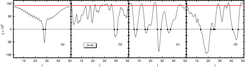
Figure 3: (Color online) The quantity ${\xi}_{1}^{i}$ [Eq.(28)] is plotted as a function of lattice site $j$ for some typical symmetry-broken GHF-determinants $|D_{1}^{i}\rangle$ resulting from the GHF-FED VAP optimization for the half-filled lattice with $N_{sites}=50$ and $U=4t$. The UHF spin-density wave is plotted in red for comparison. For more details, see the main text.

$$E_{m}^{n_{m}\Theta}=\frac{f^{n_{m}\Theta\dagger}{\mathcal{H}}^{n_{m}\Theta}f^{n_{m}\Theta}}{f^{n_{m}\Theta\dagger}{\mathcal{N}}^{n_{m}\Theta}f^{n_{m}\Theta}}$$ (20)

where the Hamiltonian ${\mathcal{H}}^{n_{m}\Theta}$ and norm ${\mathcal{N}}^{n_{m}\Theta}$ kernels account for the fact that $m-1$ linearly independent solutions have been removed from the variational space. The kernel expressions are slightly more involved than the ones in Eqs.(II.1) and (II.2.1) but still can be obtained straightforwardly. The variation with respect to the coefficients $f_{m}^{i\Theta}$ leads to a generalized eigenvalue equation similar to Eq.(10) with the constraint $f^{n_{m}\Theta\dagger}{\mathcal{N}}^{n_{m}\Theta}f^{n_{m}\Theta}=1$, while the unrestricted minimization with respect to the last added GHF-transformation ${\mathcal{D}}_{m}^{n_{m}}$ is carried out via the Thouless theorem.

The GHF-EXC-FED scheme outlined in this section provides, for each set of symmetry quantum numbers $\Theta$, a (truncated) basis of $m$ (orthonormalized) states $|\varphi_{1K}^{n_{1}\Theta}\rangle,\dots,|\varphi_{mK}^{n_{m}\Theta}\rangle$, each of them expanded by $n_{1}$, $\dots$,$n_{m}$ non-orthogonal symmetry-projected GHF-determinants, respectively. Finally, the diagonalization of the Hamiltonian Eq.(1) in such a basis

$$\sum_{j=1}^{m}\Big{[}\langle\varphi_{i}^{n_{i}}|\hat{H}|\varphi_{j}^{n_{j}}\rangle-{\epsilon}_{\alpha}^{\Theta}{\delta}_{ij}\Big{]}C_{j\alpha}^{\Theta}=0$$ (21)

provides ground and excited states

$$|{\Omega}_{\alpha}^{\Theta}\rangle=\sum_{j=1}^{m}C_{j\alpha}^{\Theta}|\varphi_{j}^{n_{j}}\rangle$$ (22)

which may account for additional correlations. Nevertheless, because many of these correlations have already been accounted for in the MR expansion of each of the $m$ basis states (as discussed above), one may expect the role of this final diagonalization to be, in general, less important than in the scheme used in Ref. 36.

Both the GHF-FED and GHF-EXC-FED VAP approximations could be extended to the use of general Hartree-Fock-Bogoliubov (HFB) transformations. Carlo-review This, however, would require an additional particle number symmetry restoration that increases our numerical effort by around one order of magnitude and has hence not been included in the present study.

II.3 Spectral functions and density of states

In this section, we briefly discuss the computation of the SFs and DOS within our theoretical framework. Let us assume that for an $N_{e}$-electron system we have already obtained, along the lines described in Sec.II.2.1, a GHF-FED ground state solution $|\phi_{1K}^{n_{1}\Theta}\rangle$. For all the lattices considered in the present study the ground state has spin $S=0$ but not necessarily linear momentum zero [i.e., $\Theta=(0,k)$]. In all cases, the ground state transforms as an irrep of dimension 1. Therefore, for this specific case, we can simply write the ground state wave function as $|n_{1},N_{e},k\rangle$. The ground state energy will be denoted as $E^{n_{1}k}$.

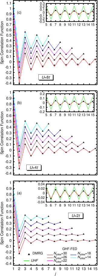
Figure 4: (Color online) GHF-FED ground state spin-spin correlation functions in real space for half-filled lattices of different sizes (red, brown, magenta, blue and cyan curves). DMRG values are plotted with black triangles. Results are shown for U=$2t$ (a), $4t$ (b) and $8t$ (c). In each panel, the inset displays a close-up of the long-range behavior predicted by the GHF-FED (red curve) and DMRG (black triangles) schemes compared with the one obtained within the standard UHF approximation (green curve) in the case of the $N_{sites}$=30 lattice. For more details, see the main text.

Usually, the SFs are defined as the imaginary part of the time-ordered Green’s function and can be calculated from the Lehmann representation. Fetter-W In order to compute them, we approximate Rayner-2D-Hubbard-PRB-2012 ; Carlos-Hubbard-1D the ground states of the ($N_{e}\pm 1$)-electron systems with the quantum numbers ${\Theta}^{\pm}=(1/2,k^{\pm})$. For the $(N_{e}-1)$-electron system we superpose the Goldstone (hole) manifolds $\hat{R}(\Omega)\hat{R}(g)\hat{b}_{h}({\mathcal{D}}_{1}^{i})|{\mathcal{D}}_{1}^{i}\rangle$ in the ansatz

$$|n_{T},N_{e}-1,k^{-}\rangle=\sum_{ihM}f_{hM}^{i{\Theta}^{-}}\hat{P}_{KM}^{{\Theta}^{-}}\hat{b}_{h}({\mathcal{D}}_{1}^{i})|{\mathcal{D}}_{1}^{i}\rangle$$ (23)

where $i=1,\dots,n_{T}$. The number $n_{T}$ of GHF-transformations used to expand the state Eq.(23) may be different from the one (i.e., $n_{1}$) in the GHF-FED ground state wave function. We write $\hat{b}_{h}({\mathcal{D}}_{1}^{i})$ to explicitly indicate that holes are made on different intrinsic determinants $|{\mathcal{D}}_{1}^{i}\rangle$ corresponding to the lowest-energy states of the $N_{e}$-electron system approximated by a single symmetry-projected configuration along the lines described in Sec.II.1. The hole index $h$ runs as $h=1,\dots,N_{e}$. Note, that the label $b=\pm 1$ is not explicitly written in this section, but it is taken into account whenever needed.

For the $(N_{e}+1)$-electron system we superpose the Goldstone (particle) manifolds $\hat{R}(\Omega)\hat{R}(g)\hat{b}_{p}^{\dagger}({\mathcal{D}}_{1}^{i})|{\mathcal{D}}_{1}^{i}\rangle$ and write

$$|n_{T},N_{e}+1,k^{+}\rangle=\sum_{ipM}g_{pM}^{i{\Theta}^{+}}\hat{P}_{KM}^{{\Theta}^{+}}\hat{b}_{p}^{\dagger}({\mathcal{D}}_{1}^{i})|{\mathcal{D}}_{1}^{i}\rangle$$ (24)

where the index $i$ runs again as $i=1,\dots,n_{T}$ and $p=N_{e}+1,\dots,2N_{sites}$. The mixing coefficients $f^{i{\Theta}^{-}}$ and $g^{i{\Theta}^{+}}$ are determined by solving eigenvalue equations similar to Eq.(10). This yields a maximun of $2n_{T}\times N_{e}\times d$ hole solutions with energies $E^{n_{T}k^{-}}$ and a maximum of $2n_{T}\times(2N_{sites}-N_{e})\times d$ particle solutions with energies $E^{n_{T}k^{+}}$ for each irreducible representation of the space group. The quantity $d$ is the dimension of the corresponding irreducible representations, i.e., $d=1$ for $k^{\pm}=0,\pi$ and $d=2$ for $k^{\pm}\neq 0,\pi$. The hole ${\mathcal{B}}(q,\omega)$ and particle ${\mathcal{A}}(q,\omega)$ SFs are then written in their standard form

$${\mathcal{B}}(q,\omega)= \sum_{k^{-}\sigma}|\langle n_{T},N_{e}-1,k^{-}|{\hat{c}}_{q\sigma}|n_{1},N_{e},k\rangle|^{2}$$

$$\times \delta\left(\omega-E^{n_{1}k}+E^{n_{T}k^{-}}\right)$$

$${\mathcal{A}}(q,\omega)= \sum_{k^{+}\sigma}|\langle n_{T},N_{e}+1,k^{+}|{\hat{c}}_{q\sigma}^{\dagger}|n_{1},N_{e},k\rangle|^{2}$$

$$\times \delta\left(\omega-E^{n_{T}k^{+}}+E^{n_{1}k}\right)$$ (25)

and the DOS can be computed as

$${\mathcal{N}}(\omega)=\sum_{q}\left({\mathcal{B}}(q,\omega)+{\mathcal{A}}(q,\omega)\right)$$ (26)

Due to the finite size of the considered lattices, both the hole and particle SFs consist of a finite number of $\delta$ functions with different weights. Therefore, we introduce an artificial Lorentzian width $\Gamma$ for each state.

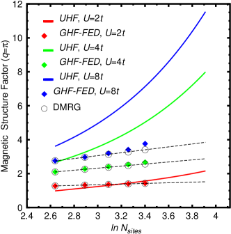
Figure 5: (Color online) The GHF-FED magnetic structure factor, evaluated at the wave vector $q=\pi$, is plotted as a function of $ln$ $N_{sites}$ for half-filled lattices of different sizes. GHF-FED results are shown for on-site repulsions of $U=2t$ (red diamonds), $4t$ (black diamonds), and $8t$ (blue diamonds). The corresponding DMRG values are plotted with open circles. A straight line has been fitted to guide the eye. The magnetic structure factors predicted by the UHF approximation for $U=2t$ (continuous red curve), $4t$ (continuous black curve), and $8t$ (continuous blue curve) are also included for comparison purposes.

III Discussion of results

In this section, we discuss the results of our calculations for some illustrative examples. In most cases, we consider on-site repulsions of $U=2t,4t$ and $8t$ representing weak, intermediate-to-strong (i.e., non-interacting band width) and strong correlation regimes. First, in Sec.III.1, we consider the ground states of half-filled lattices of various sizes. We compare our ground state and correlation energies with the exact ones, as well as with those obtained using other theoretical approaches. We then discuss the dependence of the predicted correlation energies on the number $n_{1}$ of non-orthogonal symmetry-projected configurations used to expand our ground state wave functions. The computational performance of our scheme is also addressed. The structure of the intrinsic GHF-determinants resulting from our GHF-FED VAP procedure is discussed in Sec.III.2. Our results for SSCFs in real space and MSFs, for lattices with up to 30 sites, are presented in Sec.III.3. They are compared with DMRG results. For all the considered lattices, we have retained 1024 states in the renormalization procedure. In Sec.III.4, we compare the DOS provided by our theoretical framework with the exact one, obtained with an in-house full diagonalization code in a lattice with $N_{sites}=10$. Hole SFs are also discussed in the case of $N_{sites}=30$. Finally, in Sec.III.5, we present results obtained for the excitation spectra in lattices with $N_{sites}=12,14$ and $20$ and also discuss the structure of the underlying symmetry-broken GHF-determinants resulting from our GHF-EXC-FED VAP procedure for excited states.

III.1 Ground state and correlation energies

Let us start by considering lattices of 12 and 20 sites with the GHF-FED scheme discussed in Sec.II.2.1. The corresponding $\Theta=(0,\pi)$ ground states have $B_{1}$ symmetry, i.e., they are symmetric under the reflection $x\rightarrow-x$. In Table I, we compare the predicted ground state energies with the exact ones. For completeness, we also include energies provided by the standard (i.e., one transformation) restricted (RHF) and unrestricted (UHF) HF frameworks. Ours is a VAP approach whose quality can be checked by studying how well it reproduces the exact ground state correlation energies. To this end, we consider the ratio

$$\kappa_{GHF-FED}=\frac{E_{RHF}-E_{GHF-FED}}{E_{RHF}-E_{EXACT}}\times 100$$ (27)

between the GHF-FED and the exact correlation energies. For the UHF approximation, $\kappa_{UHF}$ is obtained from a similar expression.

We observe from Table I that the inclusion of $n_{1}$=10 non-orthogonal symmetry-projected configurations with the GHF-FED approach significantly improves correlation energies with respect to UHF. In fact, $\kappa_{GHF-FED}\geq 99.79\%$ in all considered correlation regimes even for $N_{sites}=20$ which is out of reach with exact diagonalization.

In the case of $N_{sites}=14$, whose $\Theta=(0,0)$ ground state has $A_{1}$ symmetry, i.e., it is symmetric under the reflection $x\rightarrow-x$, our calculations with $n_{1}=10$ transformations predict energies of $-11.9539t$, $-8.0874t$, and $-4.6127t$ compared to the exact ones of $-11.9543t$, $-8.0883t$, and $-4.6131t$ for $U=2t,4t,$ and $8t$, respectively. This yields $\kappa_{GHF-FED}$ values of $99.95,99.97$, and $99.99\%$, respectively. Results for this lattice have been reported in the literature with the ResHF framework using the half-projection method. Ikawa-1993 For half-filled lattices with sizes comparable to the ones already mentioned, the Gutzwiller method Gutzwiller_method provides $\kappa$ ratios around $85,77,$ and $50\%$, respectively.Gutzwiller1 ; VMC-Yokoyama Let us also mention that our GHF-FED energies for $N_{sites}=12$ and $14$ improve upon previously reported VAP values of $-6.9093t$ and $-8.0577t$ for $U=4t$. Carlos-Hubbard-1D

Calculations have also been carried out for $N_{sites}=16$, whose $\Theta=(0,\pi)$ ground state has $B_{1}$ symmetry. We have obtained ground state energies of $-16.4754t$ for $U=t$ and $-9.2122t$ for $U=4t$ while the exact ones are $-16.4758t$ and $-9.2144t$, respectively. Previous DMRG results for this lattice, have been reported in the literature. Xiang For all the lattices with sizes $N_{sites}$ $\leq$ 18 our DMRG calculations, retaining 1024 states in the renormalization procedure, reproduce the exact Lieb-Wu ground state energies (to all quoted figures) for the considered U values.

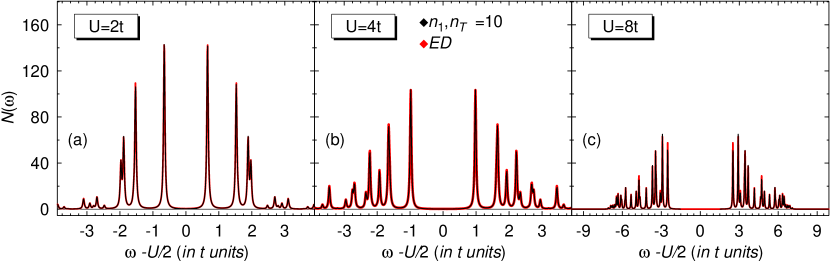
Figure 6: (Color online) The DOS (black) for the half-filled lattice with $N_{sites}=10$ at $U=2t,4t,$ and $8t$ is plotted in panels (a), (b), and (c), respectively, as a function of the shifted excitation energy $\omega-U/2$ (in $t$ units). Results have been obtained by approximating the $N_{e}$ and $(N_{e}\pm 1$)-systems with $n_{1}=10$ and $n_{T}=10$ GHF-determinants. Our results are hardly distinguishable from the DOS obtained with exact diagonalization (red). A Lorentzian folding of width $\Gamma=0.05t$ has been used. For more details, see the main text.

The ground state energies for the lattices with $N_{sites}=30$ and $50$ are compared in Table II with the exact ones. In this case, the corresponding $\Theta=(0,0)$ ground states have $A_{1}$ symmetry. In the same table, we also present ground state energies predicted with the ResHF method Tomita-1 based on $n_{1}=30$ UHF-transformations (i.e., UHF-ResHF). It is very satisfying to observe that both the GHF-FED and the UHF-ResHF VAP schemes can account for $\kappa\geq 98\%$ in a relatively large lattice with $N_{sites}=30$. In fact, the GHF-FED scheme provides $\kappa\geq 99.39\%$ with 45,048 variational parameters that represents a small fraction of the dimension of the restricted (i.e., accounting for all symmetries) Hilbert space in this lattice. In this case, our GHF-FED energy also improves the variational value $-16.6060t$ obtained in Ref. 35 for $U=4t$ using a single symmetry-projected configuration. Note, that the ResHF method Fukutome-original-RSHF ; Tomita-1 is not intrinsically limited to the use of UHF-transformations and, therefore, the UHF-ResHF ground state energies shown in Table II can still be improved by, for example, adopting GHF-transformations as basic building blocks. Tomita-2011PRB On the other hand, for $N_{sites}=30$ our DMRG calculations provide the energies $-25.3830t$, $-17.2334t$, and $-9.8387t$ for $U=2t,4t,$ and $8t$, respectively.

Let us now comment on our results for $N_{sites}=32$ whose $\Theta=(0,\pi)$ ground state has $B_{1}$ symmetry. We have used $n_{1}=25$ GHF-transformations. For on-site repulsions of $U=t$ and $2t$, we have obtained energies of $-33.2137t$ and $-26.9814t$ while the UHF-ResHF ones Tomita-1 are $-33.2128t$ and $-26.9556t$, respectively. These energies, should be compared with the exact ones of $-33.2152t$ and $-27.0183t$ as well as with the DMRG values $-33.2141t$ and $-27.0177$. For previous DMRG calculations for this lattice the reader is referred to Ref. 62.

From the previous results, we conclude that the GHF-FED approximation can be considered a reasonable starting point for building correlated ground state wave functions which, at the same time, respect the original symmetries of the 1D Hubbard Hamiltonian. This is further corroborated from the results, shown in Table II, for $N_{sites}=50$. In particular, even when our description of the ground state in this lattice is poorer than in the $N_{sites}=30$ case since we have kept the same number of GHF-transformations, it is remarkable that we obtain (with 125,048 variational parameters) the values $\kappa_{GHF-FED}=96.46,95.19,$ and $98.65\%$, respectively. For the same on-site repulsions the variational Monte Carlo method VMC-Yokoyama predicts $\kappa$ values of around $87,92,$ and $96\%$. The corresponding UHF-ResHF values Tomita-1 are also listed in Table II.

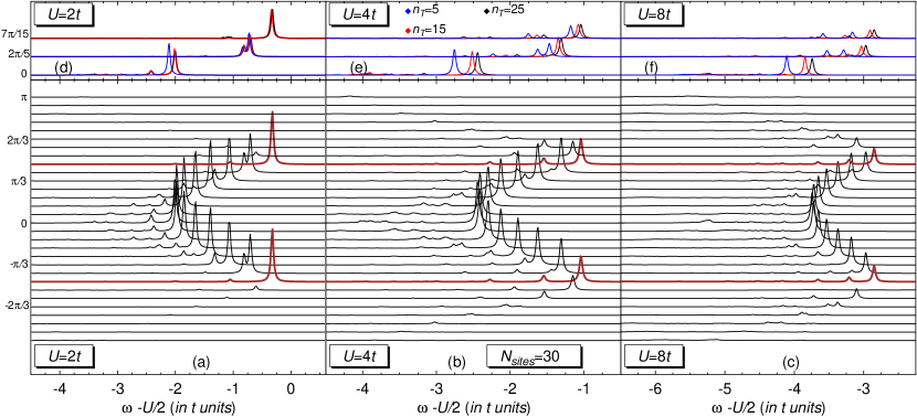
Figure 7: (Color online) The hole SFs for the half-filled lattice with $N_{sites}=30$ at $U=2t,4t,$ and $8t$ are plotted in panels (a), (b), and (c) as functions of the shifted excitation energy $\omega-U/2$ (in $t$ units). Results have been obtained by approximating the $N_{e}$ and $(N_{e}\pm 1$)-systems with $n_{1}=25$ and $n_{T}=25$ GHF-determinants. The hole SFs for momenta identical to the Fermi momentum are displayed in brown color. The shapes of some selected hole SFs (i.e., $k=0,2\pi/5$ and $7\pi/15$), obtained by approximating the ground states of the $(N_{e}\pm 1$)-systems with $n_{T}=5$ (blue), $15$ (red) and $25$ (black) but the ground state of the $N_{e}$-system always with $n_{1}$=25 GHF-transformations, are compared in panels (d), (e), and (f). A Lorentzian folding of width $\Gamma=0.05t$ has been used. For more details, see the main text.

In Fig.1, we have plotted the ratio $\kappa_{GHF-FED}$, as a function of the inverse $1/n_{1}$ of the number of transformations $n_{1}$ included in the GHF-FED ansatz, for lattices with $N_{sites}=20$ and $30$. They increase smoothly with the number of non-orthogonal symmetry-projected configurations used to expand the wave function. From Fig.1, it is apparent (see also Tables I and II) that with increasing lattice size, we need a larger number $n_{1}$ of symmetry-projected configurations to keep and/or improve the quality of the GHF-FED wave functions. For example, comparing the $N_{sites}=20$ and $30$ lattices, we see that in the former $n_{1}=10$ transformations are enough to obtain $\kappa_{GHF-FED}\geq 99.79\%$ while in the latter $98.69\%\leq\kappa_{GHF-FED}\leq 99.49\%$. On the other hand, in the $N_{sites}=50$ case, $n_{1}=10$ transformations leads to $93.37\%\leq\kappa_{GHF-FED}\leq 97.68\%,$ whereas with $n_{1}=25$ we reach the $\kappa_{GHF-FED}$ values shown in Table II.

Obviously, as in many other approaches to many-fermion systems, we are always limited to a finite number of configurations in practical calculations. Nevertheless, the GHF-FED scheme provides compact ground state wave functions whose quality can be systematically improved by adding new (variationally determined) non-orthogonal symmetry-projected configurations. In fact, both ours and the ResHF Yamamoto-2 ; Ikawa-1993 ; Tomita-1 wave functions are nothing else than a discretized form of the exact coherent-state representation of a fermion state Perlemov and, therefore, become exact in the limit $n_{1}\rightarrow\infty$. Our aim in the present work is not to lower the ground state energy as much as possible but to test to which extent our scheme can account for relevant correlations in the considered lattices. Therefore, for the largest lattices here studied (i.e., $N_{sites}=30$ and $50$), we have restricted ourselves in practice to a maximun number $n_{1}=25$ of GHF-transformations.

A few words concerning the computational performance of our method are in order here. In panel (a) of Fig.2, we have plotted the speedup of a typical calculation as a function of the number of proccessors. Results are shown for $N_{sites}=50$ and $U=4t$ but similar behavior was also obtained for $U=2t$ and $8t$. As demonstrated in the plot, the GHF-FED speedup grows linearly with the number of processors used in the calculations. On the other hand, panel (b) of the same figure shows that (for a fixed number of proccessors) an efficient implementation of our variational scheme scales linearly with the number $n_{1}$ of GHF-transformations used while the ResHF scaling is quadratic. Concerning the scaling of our method with system size, Fig.1 shows that as the system becomes larger a larger number of transformations is required to keep the quality of our wave functions. We cannot currently determine how the number of transformations scales with system size as this would require to consider larger lattices than the ones studied in this paper.

III.2 Structure of the intrinsic determinants and basic units of quantum fluctuations

An interesting issue is whether there is any relevant information in the symmetry-broken (i.e., intrinsic) determinants $|{\mathcal{D}}_{1}^{i}\rangle$ resulting from the GHF-FED VAP optimization. We are interested in comparing the structure of these determinants with the spin-density wave solution obtained with the standard UHF approximation. Here, one should keep in mind that a variationally optimized GHF-determinant has the same energy as the optimal UHF one. Bach-Lieb-Solovej We have studied the quantity

$${\xi}_{1}^{i}(j)=(-)^{j-1}\langle{\mathcal{D}}_{1}^{i}|\mathbf{S}(j)|{\mathcal{D}}_{1}^{i}\rangle\cdot\langle{\mathcal{D}}_{1}^{i}|\mathbf{S}(1)|{\mathcal{D}}_{1}^{i}\rangle$$ (28)

where $j=1,\dots,N_{sites}$ is the lattice index while $i=1,\dots,n_{1}$ enumerates the GHF-determinants in the GHF-FED ground state (subscript $1$) solution. Among the $n_{1}=25$ transformations ${\mathcal{D}}_{1}^{i}$ used for the $N_{sites}$=50 lattice, we have selected some typical examples to plot the quantity ${\xi}_{1}^{i}(j)$. Results are displayed in panels (a) to (d) of Fig.3. Other determinants $|{\mathcal{D}}_{1}^{i}\rangle$, not shown in the figure, exhibit the same qualitative features. Similar results are also found for other on-site repulsions, as well as for other lattices.

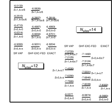
Figure 8: The energies of some selected states obtained within the GHF-EXC-FED approximation for the half-filled lattices with $N_{sites}=12$ and $14$ are compared with the ones provided by single-reference VAP (SR VAP) calculations (only 3D spin and linear momentum projections) as well as with the exact ones from Lanczos diagonalization. Carlos-Hubbard-1D Results are shown for $U=4t$.

For the standard UHF spin-density wave solution, the quantity ${\xi}_{1}^{i}(j)$ has nearly constant positive values plotted with red lines in Fig.3. A very different behavior appears in the intrinsic GHF-determinants $|{\mathcal{D}}_{1}^{i}\rangle$ associated with the GHF-FED solution. First, we observe a broad spin feature distributed all over the lattice, which is a consequence of the richer spin textures provided by the use of GHF-transformations and full 3D spin projection. In addition, pairs of points (black squares) appear where ${\xi}_{1}^{i}(j)$ changes its sign (i.e., the spin-density wave reverses it phase). These defects of the spin-density wave phase represent soliton-antisoliton ($S-\overline{S}$) pairs in the case of half-filled lattices. Yamamoto-1 ; Ikawa-1993 ; Tomita-1 ; Horovitz In particular, our analysis of the charge densities $\rho_{1}^{i}(j)=1-\sum_{\sigma}\langle{\mathcal{D}}_{1}^{i}|\hat{n}_{j\sigma}|{\mathcal{D}}_{1}^{i}\rangle$ reveal that they correspond to neutral $S^{0}-\overline{S^{0}}$ pairs. Let us stress that the presence of at least one $S^{0}-\overline{S^{0}}$ pair is a genuine VAP effect appearing even if we approximate a given ground state within a SR framework, non-unitary-paper-Carlos as discussed in Sec.II.1.

Furthermore, Fig.3 illustrates how the $S^{0}-\overline{S^{0}}$ pairs appear at different lattice locations $j$ with varying distance $R_{S^{0}-\overline{S^{0}}}$ among the members of the pairs. The latter represents the breathing motion of the $S^{0}-\overline{S^{0}}$ pairs. The $S^{0}-\overline{S^{0}}$ pairs are present in all the intrinsic determinants $|{\mathcal{D}}_{1}^{i}\rangle$ associated with the GHF-FED expansion, which as already mentioned above, superposes the Goldstone manifolds $\hat{R}_{S}(\Omega)\hat{R}(g)|{\mathcal{D}}_{1}^{i}\rangle$ containing defects in the spin-density wave. We are then left with an intuitive physical picture in which the soliton pairs can be regarded as basic units of quantum fluctuations in our GHF-FED states. On the other hand, the interference between $S^{0}-\overline{S^{0}}$ pairs belonging to different symmetry-broken determinants $|{\mathcal{D}}_{1}^{i}\rangle$ is accounted for in our calculations through a resonon-like equation similar to Eq.(10). This interpretation has been suggested in previous studies with the ResHF method. Yamamoto-1 ; Yamamoto-2 ; Ikawa-1993 ; Tomita-1

III.3 Spin-spin correlation functions and magnetic structure factors

Let us now consider the ground state spin-spin correlation functions (SSCFs) in real space. For a given set of symmetry quantum numbers $\Theta$, they can be computed as

$${\mathcal{F}}_{m}^{n_{1}\Theta}(j)=\frac{\langle\phi_{1K}^{n_{1}\Theta}|\mathbf{S}(j)\cdot\mathbf{S}(1)|\phi_{1K}^{n_{1}\Theta}\rangle}{\langle\phi_{1K}^{n_{1}\Theta}|\phi_{1K}^{n_{1}\Theta}\rangle}$$ (29)

Note that if a wave function has good spin, as it is the case with the GHF-FED one, the SSCFs have to be the same for all the members of a (2S+1)-multiplet and, therefore, they cannot depend on the $\Sigma$ quantum number. However, a dependence with respect to the particular row $m$ of the space group irreducible representation that we are using in the projection still remains and is explicitly included in ${\mathcal{F}}_{m}^{n_{1}\Theta}(j)$.

The SSCFs corresponding to the ground states for $N_{sites}=14,18,22,26,$ and $30$, approximated by $n_{1}=10,10,15,25,$ and $25$ GHF-transformations, respectively, are depicted in panels (a), (b) and (c) of Fig.4. In the same figure, we have also plotted the values resulting from our DMRG calculations. We observe a good agreement between the GHF-FED and DMRG SSCFs with slight deviations for the $N_{sites}=30$ lattice at U=8t, which can be improved by increasing the number of transformations. In particular, both SSCFs display a rapid decrease for $j\leq 3$. A similar feature has been studied in previous works. Tomita-1 ; Yamamoto-1 ; Yamamoto-2 ; Ikawa-1993 ; Shiba-Pincus Regardless of the on-site interaction, the short range part of the SSCFs runs parallel for the lattices considered in Fig.4, pointing to converged behavior as a function of lattice size. Morevover, the mid and long range amplitude of the SSCF for a given lattice increases with increasing $U$ values.

In each panel of Fig.4, the inset displays a close-up of the long range behavior of the SSCF predicted by the GHF-FED and DMRG approximations compared with the one obtained within the standard UHF approach for $N_{sites}=30$. As can be observed, the amplitude of the UHF SSCF remains constant for $j\geq 5$ while the GHF-FED and DMRG ones exhibit a damped long range trend. Previous studies have suggested that there are two important ingredients necessary to account for a qualitatively correct long range behavior of the SSCFs: the self-consistent optimization of the intrinsic determinants (i.e., orbital relaxation Yamamoto-1 ; Ikawa-1993 ) and having pure spin states (i.e., no spin contamination Tomita-1 ). Our wave functions meet both conditions.

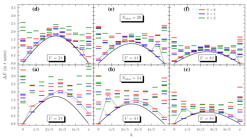
Figure 9: (Color online) Energy spectrum obtained via Eq.(21) for the half-filled lattices with $N_{sites}=14$ [panels (a), (b), and (c)] and $20$ [panels (d), (e), and (f)]. For each irreducible representation of the space group, the lowest-energy and first excited states with the spins $S=0$ (red bars),$1$ (blue bars), and $2$ (green bars) have been plotted. Results are shown for $U=2t,4t,$ and $8t$. The exact dispersion curves exactkdisp for $N_{sites}\rightarrow\infty$ (thin black lines) are also included. In order to guide the eye, the lowest-lying states with spin $S=0$ ($S=1$) have been connected by long (short) dashed lines. For more details, see the main text.

The magnetic structure factors (MSFs), evaluated at the wave vector $q=\pi$, can be computed as

$$S_{m}^{n_{1}\Theta}(\pi)=\frac{1}{N_{sites}}\sum_{ij}(-)^{i+j}\frac{\langle\phi_{1K}^{n_{1}\Theta}|\mathbf{S}(i)\cdot\mathbf{S}(j)|\phi_{1K}^{n_{1}\Theta}\rangle}{\langle\phi_{1K}^{n_{1}\Theta}|\phi_{1K}^{n_{1}\Theta}\rangle}$$ (30)

and the ones corresponding to the ground states for $N_{sites}=14,18,22,26,$ and $30$ are displayed in Fig.5 as functions of $ln$ $N_{sites}$. The corresponding DMRG results are shown in the same plot. We have also included the UHF MSFs for comparison purposes. At variance with the UHF MSFs which diverge exponentially, both the GHF-FED and DMRG results display an almost linear behavior. A previous workImada1overrMSF has shown that the SSCFs in real space behave for a half-filled system as $\approx(ln^{\sigma}j)/j$. This implies that as a funcion of the lattice size, the MSFs should behave as $ln^{1+\sigma}$ $N_{sites}$. In Fig.5, we have simply fitted a straight line using the DMRG MSFs to guide the eye. We have not attempted to determine logarithmic corrections as this would require larger lattices than those studied in the present paper.

III.4 Spectral functions and density of states

In panels (a), (b), and (c) of Fig.6, we have plotted (black) the DOS ${\mathcal{N}}(\omega)$ for $N_{sites}=10$. In the same figure, we have also plotted (red) the exact DOS obtained with an in-house full diagonalization code. There is excellent agreement between ours and the exact DOS concerning the position and relative heights of all the prominent peaks. Both ours and the exact DOS exhibit the particle-hole symmetry well known for half-filled systems text-Hubbard-1D and a splitting into the lower and upper Hubbard bands. The Hubbard gap between these bands increases with larger $U$. Both dynamical cluster approximation moukouri2001 ; huscroft2001 ; aryanpour2003 and cellular dynamical mean field theory AraGo studies suggest that this gap is preserved for any finite value of the on-site interaction at sufficiently low temperatures even in the thermodynamic limit, with $U=0t$ being the only singular point.

Tendencies to spin-charge separation as well as other relevant shadow features inside the Brillouin zone, similar to the ones expected in the infinite-$U$ limit of the 1D Hubbard model, PENcPRL1996 have been found in previous cellular dynamical mean field theory AraGo and cluster perturbation theory Senechal-scs studies of the spectral weigths in the case of finite on-site repulsions. In panels (a), (b), and (c) of Fig.7, we have plotted the hole SFs for the $N_{sites}=30$ lattice.

The first feature observed from Fig.7 is the Hubbard gap opening at the Fermi momentum $k_{F}=7\pi/15$. The spectral weight concentrates on the prominent peaks belonging to the spinon band. Our calculations for smaller lattices with $N_{sites}=14$ and $20$ indicate that this spinon band is quite stable in terms of lattice size although the relative height of its peaks decreases for increasing $U$ values. The holon singularities are clearly visible in some of the SFs shown in Fig.7 for linear momenta $-\pi/2<k<\pi/2$. On the other hand, the holon bands can also be followed for linear momenta $k>\pi/2$ and $k<-\pi/2$. They are the mirror images of the ones with opposite $\omega-U/2$ values Senechal-scs and become apparent for $U=4t$ and $8t$. However, besides the spinon band, the most relevant feature in our SFs is the very extended distribution of the spectral weight for linear momenta $-\pi/2<k<\pi/2$. The comparison with our SFs for $N_{sites}=14$ and $20,$ obtained with $n_{1}=10$ and $n_{T}=10$ GHF-transformations, reveals that the increase of lattice size produces more pronounced shadow features due to the fragmentation of the spectral strength over a wider interval of $\omega-U/2$ values. The previous finite size results show that our SFs exhibit tendencies beyond a simple quasiparticle distribution and agree qualitatively well with the ones obtained using other approximations. AraGo ; Senechal-scs

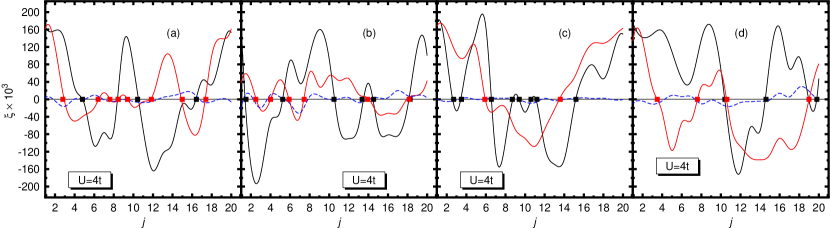
Figure 10: (Color online) Structure of some typical symmetry-broken GHF-determinants $|{\mathcal{D}}_{1}^{i}\rangle$ (black) and $|{\mathcal{D}}_{2}^{i}\rangle$ (red) used to expand the lowest-energy and first excited states with spin $S=1$, linear momentum $k=0$ and $A_{1}$ symmetry. The charge density (dashed blue) corresponding to the determinants $|{\mathcal{D}}_{2}^{i}\rangle$ is also included in each panel. Results are shown for the half-filled lattice with $N_{sites}=20$ at $U=4t$. For more details, see the main text.

The shapes of some selected hole SFs are compared in panels (d), (e), and (f) of Fig.7. As can be seen from panel (d), $n_{T}=15$ transformations are enough to account for all relevant details of the SFs shown in panel (a) for $U=2t$. On the other hand, panels (e) and (f) show that a larger number of transformations is required for $U=4t$ and $8t$. In particular, increasing the number of transformations for the ($N_{e}\pm 1$)-systems from $n_{T}=5$ to $n_{T}=15$ and/or $25$ leads to a shift of the main peaks and redistributes the spectral strength of some of the peaks found in the SFs for $n_{T}=5$ as a result of the small number of configurations used in the calculations. This explains the differences between ours and the SFs reported, for the same lattice at $U=4t$, in the previous VAP study Carlos-Hubbard-1D of the 1D Hubbard model using only $n_{1}=1$ and $n_{T}=5$ GHF-transformations.

III.5 Excitation spectra

In this section, we consider the low-lying excitation spectra obtained for $N_{sites}=12,14,$ and $20$ with the GHF-EXC-FED scheme discussed in Sec.II.2.2. For each irreducible representation of the space group, we have computed the lowest-energy and first excited states with spins $S=0,1,$ and $2$. Each of these states has been approximated by $10$ non-orthogonal symmetry-projected GHF-determinants. A final $2\times 2$ diagonalization of the 1D Hubbard Hamiltonian has also been carried out. For these particular lattices, we have found that for each symmetry $\Theta$, the (Gram-Schmidt orthonormalized) ground $|\varphi_{1K}^{n_{1}=10,\Theta}\rangle$ and first excited $|\varphi_{2K}^{n_{2}=10,\Theta}\rangle$ states are very weakly coupled through the Hamiltonian. Due to this, the energies corresponding to the states $|{\Omega}_{1K}^{\Theta}\rangle$ and $|{\Omega}_{2K}^{\Theta}\rangle$ resulting from the $2\times 2$ diagonalization are almost identical to those corresponding to the basis states $|\varphi_{1K}^{n_{1}=10,\Theta}\rangle$ and $|\varphi_{2K}^{n_{2}=10,\Theta}\rangle$. However, this cannot be anticipated a priori and the final diagonalization of the Hamiltonian should always be carried out.

In Fig.8, we compare the energies of some selected states for $N_{sites}=12$ and $14$ with the ones obtained in the previous variational study Carlos-Hubbard-1D of the 1D Hubbard model where 3D spin and linear momentum projections were carried out. The exact results in Fig.8 correspond to Lanczos diagonalizations. As can be observed, our MR calculations, where in addition to 3D spin projection the full space group of the 1D Hubbard model is taken into account, improve the energies reported in Ref. 35 for both ground and excited states.

In Fig.9, we show the low-lying spectrum obtained via Eq.(21), for $N_{sites}=14$ [panels (a), (b), and (c)] and $20$ [panels (d), (e), and (f)] taken as representatives examples of systems whose $\Theta=(0,0)$ and $\Theta=(0,\pi)$ ground states have $A_{1}$ and $B_{1}$ symmetries, respectively. We observe that both the lowest-lying singlet and triplet states obtained in our calculations nicely follow the sine-like dispersion trend in the exact curve for $N_{sites}\rightarrow\infty$. The anomaly observed in the GHF-EXC-FED $k$-dispersion for the lowest-energy singlets and triplets has also been found in previous studies within the ResHF framework Ikawa-1993 as well as in finite versions of the exact Lieb-Wu solutions. Hashimoto For any finite U value, the exact $N_{sites}\rightarrow\infty$ curves exhibit gapped excitations, exception made for the $k=0$ and $k=\pi$ states which are degenerate. In our calculations such a degeneracy is broken due to finite size effects. However, we observe that for a given finite $U$ value, the energy difference between the lowest singlet and triplet states decreases with increasing lattice size. For example, for $U=2t$ we have obtained $\Delta E_{s-t}=0.5287t$ in the case $N_{sites}=14$ while $\Delta E_{s-t}=0.1275t$ for $N_{sites}=20$. For increasing on-site respulsions, irrespective of the lattice size, an overall compression of the spectra takes place. This is consistent with the fact that in the limit $U\rightarrow\infty$ all the configurations shown in Fig.9 should become degenerate.

III.6 Structure of the intrinsic determinants and basic units of quantum fluctuations in the GHF-EXC-FED wave functions

In Sec.III.2, we have discussed the structure of the intrinsic determinants associated with the GHF-FED states. Here, we pay attention to the symmetry-broken ones used to expand the GHF-EXC-FED wave functions. To illustrate our results, we consider states belonging to the spectrum shown in panel (e) of Fig.9. In particular, we have plotted in panels (a) to (d) of Fig.10 the quantities ${\xi}_{1}^{i}(j)$ (black) and ${\xi}_{2}^{i}(j)$ (red) computed [see, Eq.(28)] with some of the $n_{1}=10$ and $n_{2}=10$ symmetry-broken determinants $|{\mathcal{D}}_{1}^{i}\rangle$ and $|{\mathcal{D}}_{2}^{i}\rangle$ used to expand the lowest-energy $|\varphi_{1K}^{n_{1}=10,\Theta}\rangle$ and first excited $|\varphi_{2K}^{n_{2}=10,\Theta}\rangle$ states with $\Theta=(1,0)$ and $A_{1}$ symmetry. Other determinants, not shown in the figure, exhibit the same qualitative features. Similar results are also obtained for $U=2t$ and $8t$ as well as for other lattices.

As can be observed, both ${\xi}_{1}^{i}(j)$ and ${\xi}_{2}^{i}(j)$ display defects similar to the ones already discussed for the $S=0$ ground states provided by the GHF-FED approximation (see, Fig.3). From this we conclude that not only the ground but also the excited state wave functions provided by our MR VAP scheme superpose Goldstone manifolds built in terms of intrinsic GHF-determinants containing defects (i.e., solitons) that can be regarded as basic units of quantum fluctuations. In general, the intrinsic determinants associated with different symmetry-projected states may develop local variations of the charge density as seen (dashed blue curve) from Fig.10 where we have also plotted the quantity $\rho_{2}^{i}(j)=1-\sum_{\sigma}\langle{\mathcal{D}}_{2}^{i}|\hat{n}_{j\sigma}|{\mathcal{D}}_{2}^{i}\rangle$.

IV Conclusions

The accurate description of the most relevant correlations in the ground and low-lying excited states of a given many-fermion system, with as few configurations as possible, is a central problem in quantum chemistry, solid state, and nuclear structure physics. In the present study, we have explored a VAP MR avenue for the 1D Hubbard model. The main acomplishments of the present work are listed below.

(i) We have presented a powerful methodology of a VAP MR configuration mixing scheme, originally devised for the nuclear many-body problem, but not yet considered to study ground and excited states, with well defined symmetry quantum numbers, of the 1D Hubbard model with nearest-neighbor hopping and periodic boundary conditions. Both ground and excited states are expanded in terms of non-orthogonal and Ritz-variationally optimized symmetry-projected configurations. The simple structure of our projected states allows an efficient parallelization of our variational scheme, which scales linearly with the number of processors as well as with the number of transformations used in the calculations. The method also provides a (truncated) basis consisting of a few Gram-Schmidt orthonormalized states. This basis may be used to diagonalized the Hamiltonian to account, in a similar fashion, for additional correlations in the ground and excited states with well defined symmetry quantum numbers.

(ii) We have shown that our MR approximation gives accurate ground state energies and correlation energies as compared with the exact Lieb-Wu solutions for relatively large half-filled lattices up to $30$ and $50$ sites. The comparison with other theoretical approaches also reveals that our scheme can be considered as a reasonable starting point for obtaining correlated ground state wave functions in the case of the 1D Hubbard model. We have computed the full low-lying spectrum for the $N_{sites}=14$ and $20$ lattices. The momentum dispersion of the lowest-lying singlet and triplet states follows the exact shape predicted by the Lieb-Wu solution in the thermodynamic limit. With increasing $U$ we also observe a general compresion of the spectrum.

iii) From the analysis of the structure of the intrinsic determinants associated with our MR ground and excited state wave functions, we observe that they all contain defects (i.e., solitons) that can be regarded as basic units of quantum fluctuations for the considered lattices.

(iv) Our results for the ground state SSCFs in real space show long range decay that is not observed in the UHF case. The MSFs computed from such correlation functions show a behavior approximately linear in $ln$ $N_{sites}$ consistent with previous results available in the literature.

(v) Our approximation also allows to compute SFs and the DOS. To this end, we considered ansätze, whose flexibility is determined by the numbers $n_{1}$ and $n_{T}$ of HF-transformations used to expand the wave functions of systems with $N_{e}$ and $(N_{e}\pm 1)$-electrons. For a small lattice with $N_{sites}=10$ we have compared the DOS predicted within our approach with the one obtained using a full diagonalization and found an excellent agreement between both. For a larger lattice with $N_{sites}=30$ our scheme provides hole SFs that agree qualitatively well with the ones obtained with other approximations and exhibit tendencies beyond a simple quasiparticle distribution.

We believe that the finite size calculations discussed in the present study already show that VAP approximations, based on MR expansions in terms of non-orthogonal symmetry-projected HF-determinants, represent useful tools that complement other existing approaches to study the physics of low-dimensional correlated electronic systems. Within this context, the scheme presented in this work leaves ample space for further improvements and research. First, the number of non-orthogonal symmetry-projected configurations used in the corresponding MR expansions can be increased to improve the quality of our wave functions. Second, we could still incorporate particle number symmetry breaking (i.e., general HFB-transformations) and restoration (i.e., particle number projection) to access even more correlations. Third, our scheme can be easily extended to the 2D case as well as to doped systems with arbitrary on-site interaction strengths. Our approximation is also general enough so as to be implemented for the molecular Hamiltonian CRG-QC as well as for lattices like the honeycomb, the Kagome or the Shastry-Sutherland S-S-LAttice ones. The same VAP MR scheme can also be applied to study frustrated Hubbard models in the 1D and 2D cases. Finally, the MR scheme discussed in the present work could also be used as a powerful solver in the framework of fragment-bath embedding approximations. Knizia-Chan In particular, it could replace exact diagonalizations for fragment sizes where it is not feasible while still providing highly correlated (fragment) wave functions. Obviously, a careful analysis of the corresponding symmetries should be carried out in each case. Work along these avenues is in progress and will be reported elsewhere.

- (1) E. Dagotto, Rev. Mod. Phys. 66, 763 (1994).
- (2) J. G. Bednorz and K. A. Müller, Z. Phys. B 64, 189 (1986).
- (3) E. Dagotto, Science 309, 257 (2005).
- (4) J. Hubbard, Proc. R. Soc. (London) A 276, 238 (1963).
- (5) R. Jördens, N. Strohmaier, K. Günter, H. Moritz and T. Esslinger, Nature 455, 204 (2008); U. Schneider, L. Hackermüller, S. Will, Th. Best, I. Bloch, T. A. Costi, R. W. Helmes, D. Rasch and A. Rosch, Science 322, 1520 (2008); I. Bloch, J. Dalibard and W. Zwerger, Rev. Mod. Phys. 80, 885 (2008).
- (6) A. H. Castro Neto, F. Guinea, N. M. R. Peres, K., S. Novosolev and A. K. Geim, Rev. Mod. Phys. 81, 109 (2009).
- (7) E. H. Lieb and F. Y. Wu, Phys. Rev. Lett. 20, 1445 (1968).
- (8) H. Bethe, Z. Phys. 71, 205 (1931).
- (9) G. Fano, F. Ortolani and A. Parola, Phys. Rev. B 46, 1048 (1992).
- (10) F. H. L. Essler, H. Frahm, F. Göhmann, A. Klümper and V. E. Korepin, The One-Dimensional Hubbard Model (University Press, Cambridge, 2005).
- (11) Quantum Monte Carlo Methods in Physics and Chemistry edited by M. P. Nightingale and C. J. Umrigar, NATO Advanced Studies Institute, Series C: Mathematical and Physical Sciences (Kluwer, Dordrecht, 1999), Vol. 525.
- (12) H. De Raedt and W. von der Linden, The Monte Carlo Method in Condensed Matter Physics, edited by K. Binder (Springer-Verlag, Heidelberg, 1992).
- (13) E. Neuscamman, C. J. Umrigar and Garnet Kin-Lic Chan, Phys. Rev. B 85, 045103 (2012).
- (14) S. R. White, Phys. Rev. Lett. 69, 2863 (1992).
- (15) J. Dukelsky and S. Pittel, Rep. Prog. Phys. 67, 513 (2004).
- (16) U. Schollwöck, Rev. Mod. Phys. 77, 259 (2005).
- (17) T. Xiang, Phys. Rev. B 53, 10445 (1996).
- (18) L. Tagliacozzo, G. Evenbly and G. Vidal, Phys. Rev. B 80, 235127 (2009); C. V. Kraus, N. Schuch, F. Verstraete and J. I. Cirac, Phys. Rev. A 81, 052338 (2010); U. Schollwöck, Ann. Phys. 326, 96 (2010); G. K. -L. Chan and S. Sharma, Ann. Rev. Phys. Chem. 62, 465 (2011).
- (19) D. Zgid, E. Gull and G. Chan, Phys. Rev. B 86, 165128 (2012).
- (20) A. Georges, G. Kotliar, W. Krauth and M. J. Rozenberg, Rev. Mod. Phys. 68, 13 (1996).
- (21) T. Maier, M. Jarrell, T. Pruschke and M. H. Hettler, Rev. Mod. Phys. 77, 1027 (2005).
- (22) T. D. Stanescu, M. Civelli, K. Haule and G. Kotliar, Ann. Phys. 321, 1682 (2006).
- (23) S. Moukouri and M. Jarrell, Phys. Rev. Lett. 87, 167010 (2001).
- (24) C. Huscroft, M. Jarrell, Th. Maier, S. Moukouri and A. N. Tahvildarzadeh, Phys. Rev. Lett. 86, 139 (2001).
- (25) K. Aryanpour, M. H. Hettler and M. Jarrell, Phys. Rev. B 67, 085101 (2003).
- (26) M. Potthoff, Eur. Phys. J. B 32, 429 (2003).
- (27) G. Knizia and G. K.-L. Chan, Phys. Rev. Lett. 109, 186404 (2012).
- (28) R. F. Bishop, P. H. Y. Li, D. J. J. Farnell, J. Richter and C. E. Campbell, Phys. Rev. B 85, 205122 (2012).
- (29) P. H. Y. Li, R. F. Bishop, D. J. J. Farnell, and C. E. Campbell, Phys. Rev. B 86, 144404 (2012).
- (30) R. Rodríguez-Guzmán, J. L. Egido and L. M. Robledo, Nucl. Phys. A 709, 201 (2002)
- (31) R. Rodríguez-Guzmán, L. M. Robledo and P. Sarriguren, Phys. Rev. C 86, 034336 (2012).
- (32) P. Ring and P. Schuck, The Nuclear Many-Body Problem (Springer, Berlin, 1980).
- (33) R.R.Rodríguez-Guzmán and K.W.Schmid, Eur. Phys. J. A 19, 45 (2004).
- (34) J.-P. Blaizot and G. Ripka, Quantum Theory of Finite Fermi Systems (The MIT Press, Cambridge, MA, 1985).
- (35) K.W. Schmid, T. Dahm, J. Margueron and H. Müther, Phys. Rev. B 72, 085116 (2005).
- (36) R. Rodríguez-Guzmán, K.W. Schmid, C. A. Jiménez-Hoyos and G. E. Scuseria, Phys. Rev. B 85, 245130 (2012).
- (37) G. E. Scuseria, C. A. Jiménez-Hoyos, T. M. Henderson, K. Samanta and J. K. Ellis, J. Chem. Phys. 135, 124108 (2011).
- (38) C. A. Jiménez-Hoyos, T. M. Henderson, T. Tsuchimochi and G. E. Scuseria, J. Chem. Phys. 136, 164109 (2012).
- (39) K. Samanta, C. A. Jiménez-Hoyos and G. E. Scuseria, J. Chem. Theory Comput. 8, 4944 (2012).
- (40) K. W. Schmid, Prog. Part. Nucl. Phys. 52, 565 (2004).
- (41) H. Fukutome, Prog. Theor. Phys. 80, 417 (1988); 81, 342 (1989).
- (42) N. Tomita, Phys. Rev. B 69, 045110 (2004).
- (43) S. Yamamoto, A. Takahashi and H. Fukutome, J. Phys. Soc. Jpn. 60, 3433 (1991).
- (44) S. Yamamoto and H. Fukutome, J. Phys. Soc. Jpn. 61, 3209 (1992).
- (45) A. Ikawa, S. Yamamoto, and H. Fukutome, J. Phys. Soc. Jpn. 62, 1653 (1993).
- (46) N. Tomita and S. Watanabe, Phys. Rev. Lett. 103, 116401 (2009).
- (47) T. Mizusaki and M. Imada, Phys. Rev. B 69, 125110 (2004).
- (48) T. Mizusaki and M. Imada, Phys. Rev. B 74, 014421 (2006).
- (49) N. Tomita, Phys. Rev. B 79, 075113 (2009).
- (50) J. L. Stuber and J.Paldus, Symmetry Breaking in the Independent Particle Model. Fundamental World of Quantum Chemistry: A Tribute Volume to the Memory of Per-Olov Löwdin; Edited by E. J. Brandas and E. S Kryachko (Kluwer Academic Publishers: Dordrecht, The Netherlands, 2003).
- (51) A. L. Fetter and J. D. Walecka, Quantum Theory of Many-Particle systems (McGraw-Hill, New York, 1971).
- (52) B. Horovitz, Solitons, edited by S. E. Trullinger , V. E. Zakharov and V. L. Pokrovsky (Elsevier Science Publishers, Amsterdam, 1986).
- (53) A. F. Albuquerque et al., J. Magn. Magn. Mater. 310, 1187 (2007); B. Bauer et al., J. Stat. Mech. P05001 (2011).
- (54) For a recent account on symmetry-projection based on non-unitary HF-transformations the reader is referred to C. A. Jiménez-Hoyos, R. Rodríguez-Guzmán and G. E. Scuseria, Phys. Rev. A 86, 052102 (2012).
- (55) A.R. Edmonds, Angular Momentum in Quantum Mechanics, Princeton University Press, Princeton (1957).
- (56) N.W. Ashcroft and N.D. Mermin, Solid State Physics, Saunders College, 1976.
- (57) M.C. Gutzwiller, Phys. Rev. Lett. 10, 159 (1963).
- (58) D.C. Liu and J. Nocedal, Math. Program. B 45, 503 (1989).
- (59) W. Metzner and D. Vollhard, Phys. Rev. B 37, 7382 (1988); F. Gebhard and D. Vollhard, Phys. Rev. B 38, 6911 (1988).
- (60) H. Yokoyama and H. Shiba, J. Phys. Soc. Jpn. 56, 3582 (1987).
- (61) F. Satoh, M. Ozaki, T. Maruyama and N. Tomita, Phys. Rev. B 84, 245101 (2011).
- (62) S. Nishimoto, E. Jeckelmann and F. Gebhard, Phys. Rev. B 65, 165114 (2002).
- (63) A.M. Perlemov, Sov. Phys. Usp. 20, 703 (1977).
- (64) V. Bach, E.H. Lieb and J.P. Solovej, J. Stat. Phys. 76, 3 (1994).
- (65) H. Shiba and P. A. Pincus, Phys. Rev. B 5, 1966 (1972).
- (66) M. Imada, N. Furukawa and T. M. Rice, J. Phys. Soc. Jpn. 61, 3861 (1992).
- (67) A. Go and G. S. Jeon, J. Phys.: Condens. Matter 21, 485602 (2009).
- (68) K. Penc, K. Hallberg, F. Mila and H. Shiba, Phys. Rev. Lett. 77, 1390 (1996); J. Favan, S. Haas, K. Penc, F. Mila and E. Dagotto, Phys. Rev. B 55, R4859 (1997); A. Parola and S. Sorella, Phys. Rev. B 45, R13156 (1992); M. Ogata, T. Sugiyama and H. Shiba, Phys. Rev. B 43, 8401 (1991); Phys. Rev. B 41, 2326 (1990).
- (69) D. Sénéchal, D. Perez and M. Pioro-Ladriére, Phys. Rev. Lett. 84, 522 (2000).
- (70) F. Woynarovich, J. Phys. C 16, 5293 (1983).
- (71) K. Hashimoto, Int. J. Quant. Chem. 36, 633 (1986).
- (72) C. A. Jiménez-Hoyos, R. Rodríguez-Guzmán and G. E. Scuseria, in preparation.
- (73) B. Sutherland and B. S. Shastry, J. Stat. Phys. 33, 477 (1983).