Energy dissipation in DC-field driven electron lattice coupled to fermion baths

Abstract

Electron transport in electric-field-driven tight-binding lattice coupled to fermion baths is comprehensively studied. We reformulate the problem by using the scattering state method within the Coulomb gauge. Calculations show that the formulation justifies direct access to the steady-state bypassing the time-transient calculations, which then makes the steady-state methods developed for quantum dot theories applicable to lattice models. We show that the effective temperature of the hot-electron induced by a DC electric field behaves as $T_{\rm eff}=C\gamma(\Omega/\Gamma)$ with a numerical constant $C$, tight-binding parameter $\gamma$, the Bloch oscillation frequency $\Omega$ and the damping parameter $\Gamma$. In the small damping limit $\Gamma/\Omega\to 0$, the steady-state has a singular property with the electron becoming extremely hot in an analogy to the short-circuit effect. This leads to the conclusion that the dissipation mechanism cannot be considered as an implicit process, as treated in equilibrium theories. Finally, using the energy flux relation, we derive a steady-state current for interacting models where only on-site Green’s functions are necessary.

I Introduction

Formulating strong-field transport in electron lattice has always been one of the most challenging theoretical goals in condensed matter physics kadanoff ; mahan . This is more true with today’s advanced nano-lithography techniques where we can now realize electron lattice driven far from equilibrium. Even though this is an old problem, we are still in search of a firm theoretical paradigm to approach the problem in general. One of the central puzzles is dissipation. In equilibrium, the presence of an open environment in contact with a system introduces thermalization, and once the temperature is defined, we often use canonical or grand canonical ensemble, and do not consider the coupling to the environment as an explicit parameter. We naturally ask whether such simplifying ansatz may be possible in nonequilibrium, at least for steady-state description.

In nonequilibrium, we do not know such tremendously simplifying paradigms to take the role of the environment as an implicit parameter which can be hidden in thermalization process. On the contrary, the dissipation is considered as an integral part of the nonequilibrium process, and we need to include the dissipation mechanism explicitly for sound theoretical description. In some systems, however, the dissipation process can be simplified. In quantum dots (QDs) under a finite DC bias, electron reservoirs coupled to the QD also act as energy source/drain and the energy relaxation is assumed to happen far away from QD and inside a battery. The electrical leads are then modeled as non-interacting reservoirs, and the electron transport is viewed as a transmission problem landauer . By taking the open limit, the excess energy can be taken infinitely far away from the QD, and the problem supports steady-state doyon . Various quantum simulation methods have been proposed to study the transient behaviors of interacting models tdnrg ; werner ; schiro . In the limit where a steady-state exists, the nonequilibrium state can also be described within the time-independent statistical mechanics framework zubarev , from which Hershfield hershfield proposed the nonequilibrium density matrix

$$\hat{\rho}=\exp\left[-\beta\sum_{k}\sum_{\alpha=S,D}(\epsilon_{\alpha k}-\mu_{\alpha})\psi^{\dagger}_{\alpha k}\psi_{\alpha k}\right],$$ (1)

with the reservoir energy $\epsilon_{\alpha k}$ for the source ($\alpha=S$) and drain ($D$) with the continuum index $k$. $\psi^{\dagger}_{\alpha k}$ is the creation operator of the full scattering state as the solution of the whole system of quantum dot and the leads. $\mu_{\alpha}$ is the chemical potential of the respective reservoirs. The scattering state formulation, although conceptually appealing, has initially been applied only to limited models schiller due to the difficulty of finding the scattering states. In recent years, several steady-state methods mehta ; prl07 ; anders ; prb06 have been developed and have been extended to general models.

Recently, the attention of the field has turned to lattice nonequilbrium problems. Even at a very stage of the field, there have been important findings in the nonequilbrium processes, most notably that electrons under a DC electric field seem to build up internal energy quite quickly, reaching a quite different steady-state from equilibrium strongly correlated states freericks . One of the most popular technique of solving lattice many-body models has been the dynamical mean-field theory (DMFT) dmft . Its success has been well documented in the description of the Mott transition and strong-correlation physics in equilibrium. While there have been a fair amount of DMFT works to electric-field driven lattice systems, the validity of the local approximation is still unconfirmed and subject to intense debate.

There have been numerous attempts to simulate nonequilibrium physics in lattice models, often through isolated Hamiltonians turkowski ; freericks ; eckstein ; aoki suited for quench dynamics of cold atom systems in optical lattice, periodically driven systems aoki ; demler , and some basic dissipation models aoki ; amaricci ; aron ; aron2 ; vidmar . However, in part due to the numerical difficulties in simulating long time-evolution, most of the efforts have focused on high-field phenomena such as the dielectric breakdown in Mott insulators eckstein ; oka . The main emerging picture of the calculations is that the external field drives the electronic lattice systems into hot temperature, generally regardless of the nature of many-body interaction. Even though the picture is in agreement between many groups, the detailed understanding of the nature of the hot electron state and its eventual fate in more realistic setting is not available. To gain systematic understanding of such nonequilibrium state, the dissipation should be included in explicit models and their analytic behavior has to be studied with the damping as a controlled parameter.

One of the goals of this paper is to introduce steady-state formulation via scattering state method for lattice with fermion baths and comprehensively analyze the model to show that the system possesses many properties which are expected of physical systems, for instance, consistent picture as the Boltzmann transport theory. In the process, an argument will be made that the fermion bath model and the steady-state methods are a good minimal system to study nonequilibrium strong correlation physics. In the previous paper fbath by one of Authors, the fermion bath model under a DC electric field has been shown to reproduce the key ingredients as predicted by the classical Boltzmann transport theory, and to have a stead-state solution. The occupation number as a function of mechanical momentum has been shown to have the Fermi sea shift by the drift velocity proportional to the scattering time and the electric field. Furthermore, the DC current has been derived to be consistent with the Boltzmann transport result applied to nanostructures lebwohl .

In this work, we further develop the solution to show that the scattering state formulation is applicable, and therefore a wide range of new techniques can be developed to solve the interacting lattice nonequilibrium phenomena. Explicit calculations from temporal gauge and the Coulomb gauge with scattering state formulation show that they are completely consistent with each other. The Coulomb gauge enables the time-independent formalism, making physical interpretations more transparent. We calculate explicitly the local distribution function, from which we derive that the effective temperature scales as $T_{\rm eff}=C\gamma(\Omega/\Gamma)$ with a numerical constant $C$, tight-binding parameter $\gamma$, the Bloch oscillation frequency $\Omega$ and the damping parameter $\Gamma$. The effective temperature exhibits a singular limit of $T_{\rm eff}\to\infty$ for $\Gamma/\Omega\to 0$. This proves that one should not take the damping as an implicit process, as treated in equilibrium theory. Finally we derive, via the energy flux conservation with the Joule heating, a general DC current relation as a functional of local Green’s functions as an extension of the Meir-Wingreen formula meir to lattice models, and confirm the linear response theory.

The main text of the paper is organized as follows. In Section II, the method introduced in Ref. fbath, is further developed for Green’s functions in the temporal gauge. In Section III, we introduce the Coulomb gauge and show that the Green’s functions in both gauges become identical in the long-time limit. In Section III we further discuss several important nonequilibrium quantities: the local distribution function and the effective temperature in A, time-evolution of wave-packet in B, dissipation and energy flux in C, and finally the derivation of the DC current in interacting models in D. Appendices provide detailed analytic calculations.

II Time-dependent theory with temporal gauge

To demonstrate the equivalence of the time-dependent temporal gauge to the scattering-state formalism with time-independent Coulomb gauge, we start with the one-dimensional non-interacting model considered earlier fbath . We study a quadratic model of a one-dimensional $s$-orbital tight-binding model connected to fermionic reservoirs (see Fig. 1) under a uniform electric field $E$. The effect of the electric field for time $t>0$ is absorbed in the temporal gauge as the Peierls phase $\varphi(t)=\Omega t\cdot\theta(t)$ in the hopping integral turkowski $\gamma$. Here $\Omega=eEa$ is the Bloch oscillation frequency and $\theta(t)$ is the step function. The time-dependent Hamiltonian then reads

$$\hat{H}(t) = -\gamma\sum_{\ell}(e^{i\varphi(t)}d^{\dagger}_{\ell+1}d_{\ell}+{\rm H.c.})+\sum_{\ell\alpha}\epsilon_{\alpha}c^{\dagger}_{\ell\alpha}c_{\ell\alpha}$$ (2)

$$-\frac{g}{\sqrt{L}}\sum_{\ell\alpha}(c^{\dagger}_{\ell\alpha}d_{\ell}+{\rm H.c.}),$$

with $d^{\dagger}_{\ell}$ as the (spinless) electron operator on the tight-binding chain on site $\ell$, $c^{\dagger}_{\ell\alpha}$ with the reservoir fermion states connected to the site $\ell$ with the continuum index $\alpha$ along each reservoir chain of length $L$. The length $L$ is taken to infinity, and the time scale $L/v_{F}$ (with Fermi velocity of the chain $v_{F}$) for the wave to reach the end of the reservoir chain is considered larger than any other time scales in the problem. As discussed in Ref. fbath, , the Hamiltonian can be diagonalized in each $k$-sector as $\hat{H}(t)=\sum_{k}\hat{H}_{k}(t)$ with

$$\hat{H}_{k}(t) = -2\gamma\cos[k+\varphi(t)]d^{\dagger}_{k}d_{k}+\sum_{\alpha}\epsilon_{\alpha}c^{\dagger}_{k\alpha}c_{k\alpha}$$ (3)

$$-\frac{g}{\sqrt{L}}\sum_{\alpha}(c^{\dagger}_{k\alpha}d_{k}+{\rm H.c.}),$$

with the fermion operators Fourier transformed to the wave-vector basis. Here $\epsilon_{d}(k)=-2\gamma\cos(k)$ is the tight-binding dispersion at zero $E$-field. The reservoir states formed by $c^{\dagger}_{k\alpha}$ acts as an open particle source with its chemical potential set at zero energy. The problem can be solved with $\hat{H}_{0}=\hat{H}_{k}(0)$ as the unperturbed Hamiltonian and $\hat{V}(t)=\hat{H}_{k}(t)-\hat{H}_{k}(0)$ as the time-dependent perturbation,

$$\hat{V}(t)=-2\gamma\left\{\cos[k+\varphi(t)]-\cos(k)\right\}d^{\dagger}_{k}d_{k}\equiv v(t)d^{\dagger}_{k}d_{k}.$$ (4)

This block-diagonal Hamiltonian is nothing but a resonant level model coupled to a reservoir, with the level’s energy oscillating in time jauho . With the perturbation of one-body terms of a finite degrees of freedom, one can write the Dyson’s equation for the retarded and lesser Green’s functions as blandin ; fbath

$${\bf G}_{k}^{r} = {\bf G}_{k,0}^{r}+{\bf G}_{k,0}^{r}{\bf V}{\bf G}_{k}^{r}$$ (5)

$${\bf G}_{k}^{<} = [I+{\bf G}_{k}^{r}{\bf V}]{\bf G}_{k,0}^{<}[I+{\bf V}{\bf G}_{k}^{a}],$$ (6)

where ${\bf G}_{k}^{<}$ and ${\bf G}_{k}^{r}$ are the lesser and retarded Green’s function matrices, respectively. ${\bf G}_{k,0}^{<}$ and ${\bf G}_{k,0}^{r}$ are for the non-interacting limit. The multiplication of Green’s function matrices denotes time integration.

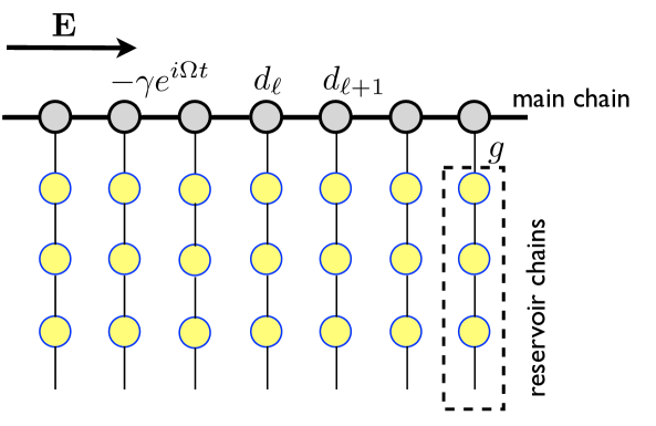
Figure 1: One-dimensional tight-binding lattice of orbital $d_{\ell}$ under an electric field $E$. Each lattice site is connected to an identical fermionic bath of $\{c_{\ell\alpha}\}$ with the continuum index $\alpha$ along the reservoir chain direction. In the temporal gauge the effect of the electric field is absorbed in the hopping integral $-\gamma$ with the Peierls phase $e^{i\Omega t}$.

Following Ref. fbath, , the retarded Green’s function is

$$G_{k}^{r}(t,t^{\prime})=-i\theta(t-t^{\prime})e^{-\Gamma|t-t^{\prime}|+2\gamma i\int_{t^{\prime}}^{t}\cos(k+\Omega s)ds},$$ (7)

with the damping parameter $\Gamma=(g^{2}/L)\sum_{\alpha}\delta(\epsilon_{\alpha})$ for reservoirs of flat density of states of infinite bandwidth. The local retarded Green’s function $G^{r}_{\rm loc}(t,t^{\prime})=(2\pi)^{-1}\int^{\pi}_{-\pi}G^{r}_{k}(t,t^{\prime})dk$ becomes

$$G_{\rm loc}^{r}(t,t^{\prime})=-i\theta(t-t^{\prime})e^{-\Gamma|t-t^{\prime}|}J_{0}\left(\frac{4\gamma}{\Omega}\sin\frac{\Omega(t-t^{\prime})}{2}\right),$$ (8)

with the zero-th Bessel function $J_{0}(x)$. Here, the gauge-invariant local function becomes a function of only the relative time, $G_{\rm loc}^{r}(t,t^{\prime})=G_{\rm loc}^{r}(t-t^{\prime})$. Fourier transformation with respect to the relative time gives

$$G^{r}_{\rm loc}(\omega)=\sum_{m=-\infty}^{\infty}\frac{J_{m}(\frac{2\gamma}{\Omega})^{2}}{\omega+m\Omega+i\Gamma},$$ (9)

by using the Bessel function relation gradshteyn $J_{0}(2z\sin\frac{\alpha}{2})=\sum_{m}[J_{m}(z)]^{2}e^{im\alpha}$.

The lesser Green’s function can be simplified in a straightforward calculation from Eq. (6) following the similar procedures as in Ref. fbath, in the long-time limit ($t,t^{\prime}\gg\Gamma^{-1}$) as

$$G_{k}^{<}(t,t^{\prime})=\int^{t}_{-\infty}ds\int^{t^{\prime}}_{-\infty}ds^{\prime}G^{r}_{k}(t,s)\Sigma_{\Gamma}^{<}(s-s^{\prime})G^{a}_{k}(s^{\prime},t^{\prime}),$$ (10)

where

$$\Sigma_{\Gamma}^{<}(s)=\int^{0}_{-\infty}\frac{i\Gamma}{\pi}e^{-i\omega s}d\omega,$$ (11)

with the self-energy ${\bf\Sigma}_{\Gamma}$ from the damping taken as the perturbation. Although the above equation has been derived with the time-dependent Peierls term Eq. (4) as the perturbation, the same result can be obtained when the damping is considered as perturbation in the limit that transient terms die out. The local lesser Green’s function can be computed as $G^{<}_{\rm loc}(t,t^{\prime})=(2\pi)^{-1}\int_{-\pi}^{\pi}G^{<}_{k}(t,t^{\prime})dk$, which again renders the Green’s function only dependent on the relative time. After changing the dummy variables $s-t\to s$ and $s^{\prime}-t^{\prime}\to s^{\prime}$, we have

$$G^{<}_{\rm loc}(\omega) = \frac{i\Gamma}{\pi}\int_{-\infty}^{\infty}dt\int_{-\infty}^{0}d\omega^{\prime}\int_{-\infty}^{0}ds\int_{-\infty}^{0}ds^{\prime}$$

$$\times e^{i(\omega-\omega^{\prime})t-i\omega^{\prime}(s-s^{\prime})+\Gamma(s+s^{\prime})}J_{0}\left(\frac{4\gamma}{\Omega}\sqrt{A}\right)$$

with

$$A = \sin^{2}\frac{\Omega s}{2}+\sin^{2}\frac{\Omega s^{\prime}}{2}-2\cos\left[\Omega\left(t+\frac{s-s^{\prime}}{2}\right)\right]$$

$$\times\sin\frac{\Omega s}{2}\sin\frac{\Omega s^{\prime}}{2}.$$

Again by utilizing the Bessel function relation gradshteyn $J_{0}(\sqrt{a^{2}+b^{2}-2ab\cos\alpha})=\sum_{m}J_{m}(a)J_{m}(b)e^{im\alpha}$

$$G^{<}_{\rm loc}(\omega) = 2i\Gamma\sum_{m}f(\omega+m\Omega)\left|\int_{-\infty}^{0}e^{-i(\omega+\frac{m\Omega}{2})s+\Gamma s}\right.$$

$$\times\left.J_{m}\left(\frac{4\gamma}{\Omega}\sin\frac{\Omega s}{2}\right)ds\right|^{2},$$

with $f(x)=\theta(-x)$, the Fermi-Dirac function at zero temperature. From the identity gradshteyn , $J_{m}(2z\sin\frac{\alpha}{2})=e^{-im(\pi-\alpha)/2}\sum_{\ell}J_{\ell}(z)J_{m+\ell}(z)e^{i\ell\alpha}$,

$$G^{<}_{\rm loc}(\omega)=2i\Gamma\sum_{m}f(\omega+m\Omega)\left|\sum_{\ell}\frac{J_{\ell}(\frac{2\gamma}{\Omega})J_{\ell-m}(\frac{2\gamma}{\Omega})}{\omega+\ell\Omega+i\Gamma}\right|^{2}.$$ (12)

Although the two Green’s functions, Eqs. (9) and (12), have been reduced to familiar forms resembling spectral representation, a clear relation between them is not available yet. In the following section, we discuss the scattering state formalism and find relations connecting the retarded and lesser Green’s functions.

III Scattering state formalism

We have learned from Ref. fbath, and the above calculations that the fermion bath model has a well-defined time-independent limit for gauge-invariant quantities such as local Green’s function. This observation and the presence of infinite reservoir states prompt us to consider scattering state formalism scattering . As depicted in Figs. 2(a), for each site on the main chain there are infinite degrees of freedom coupled from each reservoirs. Therefore, we can rewrite the quadratic Hamiltonian in terms of the scattering states originating from the fermion reservoir chains prb06 . To adopt the time-independent scattering theory, we use the Coulomb gauge as shown in Fig. 2(a) with the Hamiltonian,

$$\hat{H}_{\rm Coul} = -\gamma\sum_{\ell}(d^{\dagger}_{\ell+1}d_{\ell}+{\rm H.c.})-\sum_{\ell}\ell\Omega d^{\dagger}_{\ell}d_{\ell}$$

$$+\sum_{\ell\alpha}(\epsilon_{\alpha}-\ell\Omega)c^{\dagger}_{\ell\alpha}c_{\ell\alpha}$$

$$-\frac{g}{\sqrt{L}}\sum_{\ell\alpha}(c^{\dagger}_{\ell\alpha}d_{\ell}+{\rm H.c.}),$$

where the static Coulomb potential is applied as a potential slope to the chain and each reservoirs with their chemical potential are raised together with the corresponding tight-binding sites.

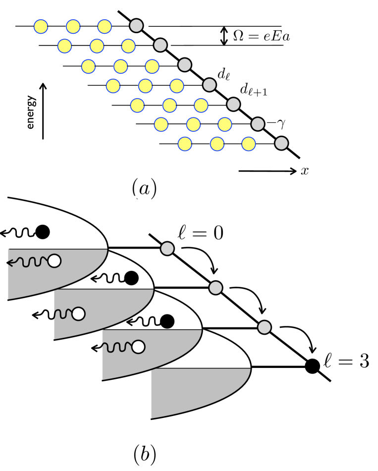
Figure 2: (a) In the Coulomb gauge for the scattering state formulation, each tight-binding sites and the associated fermion baths are on a potential slope with the potential drop between neighboring sites as $\Omega$. (b) As electron moves down the potential slope (from $\ell=0$ to $\ell=3$ in the figure), it leaves a trail of electron-hole pairs in the fermion reservoirs through particle-exchange. Since these electron-hole pairs travel indefinitely along the infinite bath chains, the reservoirs act like energy drains mimicking inelastic processes. There is an energy flux to the reservoirs, but no net particle flux.

Since the Hamiltonian is quadratic and the chain is coupled to open systems, we can decompose the Hamiltonian in terms of the scattering state operators $\psi^{\dagger}_{\ell\alpha}$ originating from the asymptotic state $c^{\dagger}_{\ell\alpha}$ as given by the Lippmann-Schwinger equation scattering ,

$$\psi^{\dagger}_{\ell\alpha} = c^{\dagger}_{\ell\alpha}+\frac{1}{\epsilon_{\alpha}-\ell\Omega-{\cal L}+i\eta}[\hat{H}_{g},c^{\dagger}_{\ell\alpha}]$$ (14)

$$= c^{\dagger}_{\ell\alpha}-\frac{g}{\sqrt{L}}\frac{1}{\epsilon_{\alpha}-\ell\Omega-{\cal L}+i\eta}d^{\dagger}_{\ell},$$

with the Liouvillian operator ${\cal L}\hat{A}=[\hat{H}_{\rm Coul},\hat{A}]$ for any operator and $\hat{H}_{g}=-(g/\sqrt{L})\sum_{\ell\alpha}(c^{\dagger}_{\ell\alpha}d_{\ell}+{\rm H.c.})$. The scattering state embodies the openness of the fermion reservoirs. As implemented by the infinitesimal imaginary poles given by $i\eta$, once the electrons scatter into a reservoir they never come back to the tight-binding chain. With the scattering state basis, the Hamiltonian is rewritten as

$$\hat{H}_{\rm Coul}=\sum_{\ell\alpha}(\epsilon_{\alpha}-\ell\Omega)\psi^{\dagger}_{\ell\alpha}\psi_{\ell\alpha},$$ (15)

with the Fermi statistics applied separately within each $\ell$-sector

$$\langle\psi^{\dagger}_{\ell\alpha}\psi_{\ell\alpha}\rangle=f(\epsilon_{\alpha}).$$ (16)

Since the Hamiltonian is quadratic, the scattering state operator $\psi^{\dagger}_{\ell\alpha}$ is a linear combination of the original basis of $d^{\dagger}_{\ell^{\prime}}$ and $c^{\dagger}_{\ell^{\prime}\alpha^{\prime}}$, and

$$\psi^{\dagger}_{\ell\alpha}=c^{\dagger}_{\ell\alpha}+\sum_{\ell^{\prime}}d^{\dagger}_{\ell^{\prime}}C_{\ell\alpha}(d_{\ell^{\prime}})+\sum_{\ell^{\prime}\alpha^{\prime}}c^{\dagger}_{\ell^{\prime}\alpha^{\prime}}C_{\ell\alpha}(c_{\ell^{\prime}\alpha^{\prime}}),$$ (17)

with the expansion coefficient for a fermion annihilation operator $a$ given as

$$C_{\ell\alpha}(a)=\{a,\psi^{\dagger}_{\ell\alpha}-c^{\dagger}_{\ell\alpha}\}=\left\{a,\frac{-g/\sqrt{L}}{\epsilon_{\alpha}-\ell\Omega-{\cal L}+i\eta}d^{\dagger}_{\ell}\right\}.$$ (18)

It is important to realize that, for a quadratic Hamiltonian, the anti-commutation of operators in $C_{\ell\alpha}(a)$ is just a c-number. In fact, this c-number is nothing but the retarded Green’s function $\overline{G}^{r}_{\ell^{\prime}\ell}(\epsilon_{\alpha}-\ell\Omega)$ between $d_{\ell^{\prime}}$ and $d^{\dagger}_{\ell}$. From this argument, the retarded Green’s function in any time-independent quadratic Hamiltonian is independent of statistics. Note that the scattering state $\psi^{\dagger}_{\ell\alpha}$ originating from the $\ell$-th reservoir has admixture from any reservoir states $c^{\dagger}_{\ell^{\prime}\alpha^{\prime}}$. Here, we have put an over-line to denote the Green’s function in the Coulomb gauge. We then have

$$\psi^{\dagger}_{\ell\alpha}=c^{\dagger}_{\ell\alpha}-\frac{g}{\sqrt{L}}\sum_{\ell^{\prime}}\overline{G}^{r}_{\ell^{\prime}\ell}(\epsilon_{\alpha}-\ell\Omega)d^{\dagger}_{\ell^{\prime}}+\cdots.$$ (19)

This equation can be inverted to express $d_{\ell}$ in terms of the scattering state basis $\psi_{\ell\alpha^{\prime}}$ as

$$d_{\ell}=\sum_{\ell^{\prime}\alpha^{\prime}}\tilde{C}_{\ell}(\ell^{\prime}\alpha^{\prime})\psi_{\ell^{\prime}\alpha^{\prime}}.$$ (20)

Similarly as above, $\tilde{C}_{\ell}(\ell^{\prime}\alpha^{\prime})=\{\psi^{\dagger}_{\ell^{\prime}\alpha^{\prime}},d_{\ell}\}$ since the scattering state operators also satisfy the anti-commutation relation prb06 $\{\psi^{\dagger}_{\ell,\alpha},\psi_{\ell^{\prime}\alpha^{\prime}}\}=\delta_{\ell\ell^{\prime}}\delta_{\alpha\alpha^{\prime}}$, and

$$d_{\ell}=-\frac{g}{\sqrt{L}}\sum_{\ell^{\prime}\alpha^{\prime}}\overline{G}^{r}_{\ell\ell^{\prime}}(\epsilon_{\alpha^{\prime}}-\ell^{\prime}\Omega)\psi_{\ell^{\prime}\alpha^{\prime}}.$$ (21)

We will discuss below how $\overline{G}^{r}_{\ell\ell^{\prime}}(\omega)$ is explicitly calculated. On-site retarded Green’s function at the central site $\ell=0$ can be expressed in terms of the scattering state basis as

$$\overline{G}^{r}_{00}(\omega) = \frac{g^{2}}{L}\sum_{\ell\alpha,\ell^{\prime}\alpha^{\prime}}\frac{\overline{G}^{r}_{0\ell}(\epsilon_{\alpha}-\ell\Omega)[\overline{G}^{r}_{0\ell^{\prime}}(\epsilon_{\alpha^{\prime}}-\ell^{\prime}\Omega)]^{*}}{\omega-\epsilon_{\alpha}+\ell\Omega+i\eta}$$ (22)

$$\times\langle\{\psi_{\ell\alpha},\psi^{\dagger}_{\ell^{\prime}\alpha^{\prime}}\}\rangle$$

$$= \frac{g^{2}}{L}\sum_{\ell\alpha}\frac{|\overline{G}^{r}_{0\ell}(\epsilon_{\alpha}-\ell\Omega)|^{2}}{\omega-\epsilon_{\alpha}+\ell\Omega+i\eta}.$$

Here the retarded Green’s functions appear on both sides of the equation, and its self-consistency will be examined below.

The lesser Green’s function can be calculated similarly as

$$\overline{G}^{<}_{\ell\ell^{\prime}}(\omega) = i\frac{2\pi g^{2}}{L}\sum_{m\alpha}\overline{G}^{r}_{\ell m}(\epsilon_{\alpha}-m\Omega)[\overline{G}^{r}_{\ell^{\prime}m}(\epsilon_{\alpha}-m\Omega)]^{*}$$ (23)

$$\times\delta(\omega-\epsilon_{\alpha}+m\Omega)\langle\psi^{\dagger}_{m\alpha}\psi_{m\alpha}\rangle$$

$$= 2i\Gamma\sum_{m}\overline{G}^{r}_{\ell m}(\omega)[\overline{G}^{r}_{\ell^{\prime}m}(\omega)]^{*}f(\omega+m\Omega),$$

where each reservoir has its own Fermi energy shifted by $\ell\Omega$ and $\langle\psi^{\dagger}_{\ell\alpha}\psi_{\ell\alpha}\rangle=f(\epsilon_{\alpha})$. The above expression is quite appealing and physically transparent. With the dissipation provided by the particle reservoirs, all electron statistics are governed by the Fermi statistics of the reservoirs and the effective tunneling between site $\ell$ and the reservoir attached at site $m$ is given by the retarded Green’s function $\overline{G}^{r}_{\ell m}$. It is noted that we use the infinite-band approximation for each fermion reservoirs so that any reservoir can provide electrons to any other tight-binding lattice sites in principle, and all possible thermal factors mix throughout the lattice.

Now, we turn to calculation of retarded Green’s functions. With the time-independent Hamiltonian, we only need to invert the matrix as $\overline{G}^{r}_{\ell\ell^{\prime}}(\omega)=[{\bf M}(\omega)^{-1}]_{\ell\ell^{\prime}}$ with

$$[{\bf M}(\omega)]_{\ell\ell^{\prime}}=(\omega+\ell\Omega+i\Gamma)\delta_{\ell\ell^{\prime}}+\gamma\delta_{|\ell-\ell^{\prime}|,1},$$ (24)

where the retarded self-energy $-i\Gamma$ is attached to each site $\ell$ of the tight-binding lattice with the potential slope. Solution to the matrix inversion can be found aoki as

$$\overline{G}^{r}_{\ell\ell^{\prime}}(\omega)=\sum_{m}\frac{J_{\ell-m}(\frac{2\gamma}{\Omega})J_{\ell^{\prime}-m}(\frac{2\gamma}{\Omega})}{\omega+m\Omega+i\Gamma},$$ (25)

which can be easily verified from ${\bf M}(\omega)\overline{\bf G}^{r}(\omega)={\bf I}$. Substituting this Green’s function into Eq. (23) gives the identical result Eq. (12) as derived from the time-dependent temporal gauge. Coming back to the retarded Green’s function, we can easily confirm the identity Eq. (22) from a straightforward calculation after substituting Eq. (25) into Eq. (22) and by using the contour integral and the completeness relation of Bessel functions. From Eq. (25), it follows that

$$\overline{G}^{r}_{\ell+k,\ell^{\prime}+k}(\omega)=\overline{G}^{r}_{\ell\ell^{\prime}}(\omega+k\Omega),$$ (26)

from which Eq. (23) satisfies

$$\overline{G}^{<}_{\ell+k,\ell^{\prime}+k}(\omega)=\overline{G}^{<}_{\ell\ell^{\prime}}(\omega+k\Omega).$$ (27)

In an interacting model, the self-energy is expressed in $G^{r,<,>}$ and inherits the same property,

$$\overline{\Sigma}^{r,<}_{\ell+k,\ell^{\prime}+k}(\omega)=\overline{\Sigma}^{r,<}_{\ell\ell^{\prime}}(\omega+k\Omega).$$ (28)

III.1 Distribution function

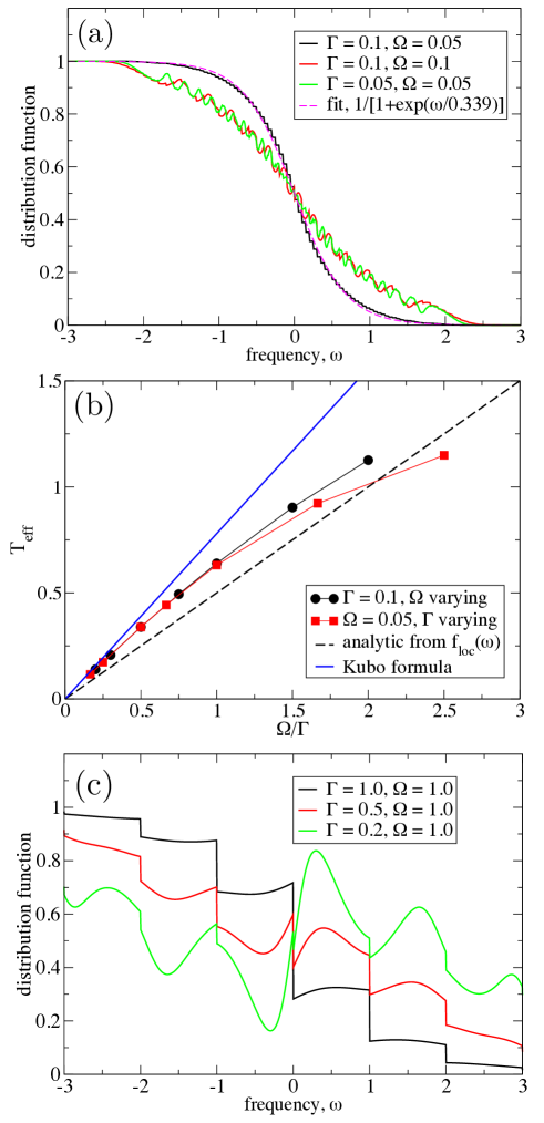
Figure 3: (a) Local distribution function $f_{\rm loc}(\omega)$ for several parameters of the damping $\Gamma$ and the Bloch oscillation frequency $\Omega$ ($\Gamma,\Omega\ll\gamma$). The effective temperature is estimated through a fit to the Fermi-Dirac function. (b) The effective temperature $T_{\rm eff}$ as a function of $\Omega/\Gamma$. Up to $\Omega/\Gamma\approx 1$, $T_{\rm eff}$ is well described as a linear function of $\Omega/\Gamma$. The dashed line denotes the analytic expression, Eq. (47), derived from the low frequency $f_{\rm loc}(\omega)$ as shown in Appendix A. The blue line is from the Kubo formula with $T_{\rm eff}=(6/\pi^{2})^{1/2}\gamma(\Omega/\Gamma)$. See Appendix B and discussions in section III.D. (c) For larger field ($\Omega=\gamma=1$), the steps become more prominent and the definition of the effective temperature becomes less robust. Nevertheless, the trend in (a-b) continues and at $\Gamma=0.2$ even a population inversion happens.

The discussion so far has demonstrated explicitly that the dissipative system with fermion baths can be described within the steady-state formalism using the scattering state basis. One of the central quantities to calculate is the effective local distribution function,

$$f_{\rm loc}(\omega)=-\frac{{\rm Im}\overline{G}^{<}_{00}(\omega)}{2{\rm Im}\overline{G}^{r}_{00}(\omega)}=\frac{\sum_{\ell}|\overline{G}^{r}_{0\ell}(\omega)|^{2}f(\omega+\ell\Omega)}{\sum_{\ell}|\overline{G}^{r}_{0\ell}(\omega)|^{2}},$$ (29)

where Eq. (22) has been used for ${\rm Im}\overline{G}^{r}_{00}(\omega)=-\Gamma\sum_{\ell}|\overline{G}^{r}_{0\ell}(\omega)|^{2}$. This result takes the same form as the ansatz considered in Aron et al. aron2 .

FIG. 3(a) shows the numerical evaluation of the local distribution function $f_{\rm loc}(\omega)$. For $\Gamma,\Omega\ll\gamma$, $f_{\rm loc}(\omega)$ is a superposition of small steps coming from the thermal factors $f(\omega+\ell\Omega)$ in Eq. (29) with the envelope following a smooth profile similar to the Fermi-Dirac function. Even though there is no reason to expect that the nonequilibrium distribution mimics the Fermi-Dirac function, we can nevertheless fit the result to the function with an effective temperature $T_{\rm eff}$ as shown, despite some deviation (see Appendix A for more details). As $T_{\rm eff}$ grows towards the finite tight-binding bandwidth $4\gamma$, the fit becomes inaccurate.

The envelope of the local distribution function plays a similar role of the Fermi-Dirac function which dictates the abundance of electron-hole pairs available for interaction. In the presence of additional many-body interactions such as the electron-phonon coupling to local optical phonons, the available electron-hole pairs for inelastic dissipation are given by the $f_{\rm loc}(\omega)$ profile and the effective temperature $T_{\rm eff}$ in the Fermi-Dirac function will play the role of hot electron temperature effectively.

It is remarkable that $T_{\rm eff}$ seems to approach infinity as the damping parameter $\Gamma$ becomes smaller. Although it may look counter-intuitive at first, this is only the manifestation of the short-circuit behavior where a finite voltage applied across a low resistance conductor induces an extremely hot temperature. This is also consistent with the numerical calculations with the general conclusion that the electron temperature reaches an infinity in closed interacting models.

Numerical fit indicates that $T_{\rm eff}$ is an increasing function of $\Omega/\Gamma$ for a wide range of $(\Omega,\Gamma)$, although the functional form eventually deviates from the form as shown in FIG. 3(b). For small $\Omega/\Gamma$, the effective temperature behaves as

$$T_{\rm eff}\approx C\gamma\left(\frac{\Omega}{\Gamma}\right),$$ (30)

with a dimensionless numerical constant $C$. This equation is one of the key results of this paper. In Appendix A, we derive the above linear dependence of $(\Omega/\Gamma)$ and approximately estimate that the constant $C\sim\frac{1}{2}$ by analyzing the $\omega=0$ step in $f_{\rm loc}(\omega)$. The effective temperature has been previously observed in the momentum distribution function and has been speculated fbath to behave as $T_{\rm eff}=\Omega^{2}/\Gamma$ based on the DC conductivity analogy. More careful and quantitative analysis now shows that the correct dependence is the above relation, Eq. (30). The $T_{\rm eff}$ relation is even further corroborated with $C$ derived from the Kubo formula (see Appendix B and discussions in section III.D.) as the blue line in FIG. 3(b). The Kubo formula result

$$T_{\rm eff}=\left(\frac{6}{\pi^{2}}\right)^{1/2}\gamma\left(\frac{\Omega}{\Gamma}\right)=0.7796\,\gamma\left(\frac{\Omega}{\Gamma}\right)$$ (31)

should be exact for the limit $\Omega/\Gamma\to 0$. The two analytical estimates bracket the numerical $T_{\rm eff}$ [see FIG. 3(b)], which shows that the expressions Eqs. (30) and (31) are a reliable approximation for $\Gamma$ and $\Omega$ up to $\gamma$.

The divergent effective temperature should be taken with a caution to interpret in finite bandwidth systems. Unlike with the quadratic dispersion relation for continuum models price , the kinetic energy in the single-band tight-binding model is always bounded and thus cannot give off extremely hot-electrons to the environment.

As $\Omega$ and $\Gamma$ become comparable to the bandwidth [see FIG. 3(c)], the signature of Bloch oscillation steps become more obvious and the definition of the effective temperature as determined by the shape of the overall $f_{\rm loc}(\omega)$ is not very robust. While the infinite temperature in a finite bandwidth system may be questionable, the trend observed in FIG. 3(a-b) continues. In the small damping limit at $\Gamma=0.2$, even a population inversion happened in the local distribution function.

III.2 Time-evolution of wave-packet

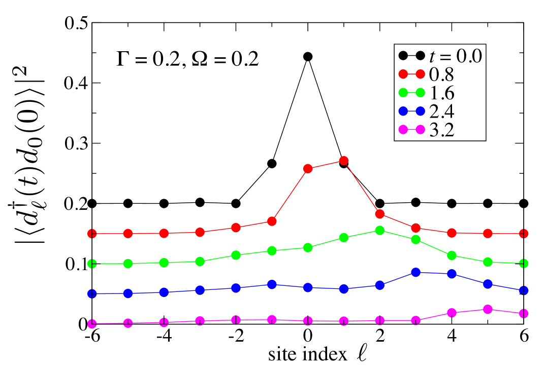
Figure 4: Observation of wave-packet evolution out of nonequilibrium steady-state. Disturbance created out of the steady-state travels down the tight-binding ladder as time evolves. The amplitude of the wave-packet diminishes due to the dephasing provided by the fermion baths. The curves have been off-set for better visibility.

So far, we have seen that the steady-state formalism provides a convenient theoretical framework for nonequilibrium lattice model of fermion baths. To better understand the nonequilibrium steady-state, we now look at time-dependent quantity indicative of wave-packet drift. A steady-state by definition is a time-independent reference state where a direct observation of time-evolution of a moving particle cannot be made. To confirm that an electric charge moves down the potential slope as a function of time, we create a hole out of occupied states create at a central position and observe its movement to a different position $x_{h}(\ell)$ as a function of time in

$$|\langle x_{h}(\ell),t|x_{h}(0),0\rangle|^{2}=|\langle d^{\dagger}_{\ell}(t)d_{0}(0)\rangle|^{2}=|G^{<}_{0\ell}(-t)|^{2}.$$ (32)

The lesser Green’s function can be easily decomposed in terms of scattering states and FIG. 4 shows the wave-packet traveling in the direction of the applied field. Amplitude of the observable decays as $e^{-2\Gamma t}$ due to the dephasing of electrons from the fermion baths.

As depicted in Fig. 2(b), electrons travel down the potential slope in the Coulomb gauge by creating a trail of electron-hole (e-h) pairs in the reservoirs. As long as the bandwidth of the reservoirs is greater than the potential drop $\Omega$ between neighboring sites (we assumed that the bandwidth is infinite in explicit calculations), each reservoirs can accommodate an e-h pair with its energy matching $\Omega$ by particle exchange via tunneling. For narrower reservoir bandwidths, multiple e-h pairs should be created to establish a DC current. Since the open reservoirs are of infinite length, the created e-h pairs travel indefinitely inside the reservoirs and therefore the fermion baths can produce effects similar to the inelastic processes in bosonic baths. We discuss this further in the subsequent sections.

III.3 Dissipation and energy flux

We turn to discussions of energy dissipation. The Hamiltonian, Eq. (III), can be divided into three parts as

$$\hat{H}_{\rm sys}=\hat{H}_{\rm TB}+\hat{H}_{\rm bath}+\hat{H}_{\rm coup},$$ (33)

with each term representing each line in Eq. (III), respectively. In the steady-state limit, the energies stored in $\hat{H}_{\rm TB}$ and $\hat{H}_{\rm coup}$ are stationary $\frac{d}{dt}\langle\hat{H}_{\rm TB}\rangle=\frac{d}{dt}\langle\hat{H}_{\rm coup}\rangle=0$, as will be demonstrated below. Unlike the case with $\hat{H}_{\rm TB}$ and $\hat{H}_{\rm coup}$ which are of finite spatial extent, the energy flux in $\hat{H}_{\rm bath}$ can be non-zero. In the scattering theory doyon , the scattering states are formulated in the limit that the spatial extent of the scattered wave ($L_{\rm scatt}$) into the reservoirs is much shorter than the length of the reservoir chain ($L_{\rm scatt}\ll L$). Therefore the scattering state represents a solution that the scattered wave constantly propagating inside the reservoirs without being backscattered from the edge of the reservoirs, and quantities involving the extended states $c^{\dagger}_{\ell k}$ or $c_{\ell k}$ do not have to be stationary in general stationary .

To be more concrete, we discuss explicit calculations. With the fermion baths, a DC electric-field establishes a DC current $J$, as calculated in Ref. fbath, . To investigate the effect of the Joule heating, we consider $\hat{H}_{\rm TB}$

$$\frac{d}{dt}\langle\hat{H}_{\rm TB}\rangle = i\left\langle[\hat{H}_{\rm Coul},\hat{H}_{\rm TB}]\right\rangle$$

$$= \Omega\langle\hat{J}\rangle+i\gamma g\sum_{\ell}\langle(\bar{c}^{\dagger}_{\ell+1}+\bar{c}^{\dagger}_{\ell-1})d_{\ell}-{\rm H.c.}\rangle$$

with the current operator $\hat{J}=i\gamma\sum_{\ell}(d^{\dagger}_{\ell+1}d_{\ell}-d^{\dagger}_{\ell}d_{\ell+1})$ within the main chain and $\bar{c}_{\ell}=(1/\sqrt{L})\sum_{\alpha}c_{\ell\alpha}$. We used the steady-state condition for the occupation $\frac{d}{dt}\langle d^{\dagger}_{\ell}d_{\ell}\rangle=0$. The first term represents the Joule heating and the second term the energy flux of electrons from the kinetic energy of the main chain into the coupling $\hat{H}_{\rm coup}$. Denoting the energy flux per site as $\hat{P}$, we show that $\langle\hat{P}\rangle=-\Omega\langle\hat{J}\rangle$. We present the detailed calculations in Appendix C and show the equality of the above equation based on the scattering-state formalism.

It can be shown further that $\frac{d}{dt}\langle\hat{H}_{\rm coup}\rangle=0$. As shown in appendix B, the energy influx to each of the reservoirs is nothing but the Joule heating

$$\frac{d}{dt}\langle\hat{h}_{\rm bath}\rangle = 2\Gamma\int\omega A_{\rm loc}(\omega)[f_{\rm loc}(\omega)-f(\omega)]d\omega$$ (35)

$$= \Omega\langle J\rangle,$$

with the local spectral function defined as

$$A_{\rm loc}(\omega)=-\frac{1}{\pi}{\rm Im}G^{r}_{00}(\omega).$$ (36)

The lowercase Hamiltonian $\hat{h}$ denotes the corresponding Hamiltonian per tight-binding site. It might sound paradoxical that the energy in the electronic system is non stationary,

$$\frac{d}{dt}\langle\hat{h}_{\rm sys}\rangle=\frac{d}{dt}\langle\hat{h}_{\rm bath}\rangle=\Omega\langle J\rangle\approx\frac{4\gamma\Gamma\Omega^{2}}{\pi(\Omega^{2}+4\Gamma^{2})}.$$ (37)

(Here the last equality is from the steady-state current taken from Ref. fbath, .) This is due to the fact that, although $\hat{H}_{\rm sys}$ governs the electron dynamics, there is another part of Hamiltonian which should be included for a closed system – the battery connected across the tight-binding chain. Since the battery loses its stored charge $Q$ with the rate of $\dot{Q}=-\langle J\rangle$, the electrostatic energy decrease per unit cell of the tight-binding chain becomes $\frac{d}{dt}\langle\hat{h}_{\rm battery}\rangle=-\Omega\langle J\rangle$, and the total energy $\hat{H}_{\rm tot}=\hat{H}_{\rm sys}+\hat{H}_{\rm battery}$ is stationary in the steady-state.

The discussion here again confirms the picture depicted in FIG. 2(b) where the fermion baths act as energy reservoirs while the net electron number flux into the reservoirs is zero. Despite their simplicity, the fermion baths through their particle-hole excitations play the role of bosonic baths, apart from the boson’s explicit dispersion relation (with the exception of the Luttinger liquid bath) and the physics that might occur from the nonlinear effect of the bosonic statistics.

III.4 Steady-state current for interacting systems

From the energy dissipation relations above, we obtain the useful formula for the steady-state current,

$$\langle\hat{J}\rangle=\frac{2\Gamma}{\Omega}\int\omega A_{\rm loc}(\omega)[f_{\rm loc}(\omega)-f(\omega)]d\omega,$$ (38)

where only on-site Green’s functions are needed as in Meir-Wingreen formula in quantum dot transport meir . To recover the Ohm’s law for small field that $\langle\hat{J}\rangle\propto\Omega$ one should have that the integral goes as $\Omega^{2}$ as the leading order. This is justified since applying a field of opposite direction $-\Omega$ should not change the local properties and the integral should be of order $\Omega^{2}$. This argument can be used to analyze the linear response limit, as described below.

The above relation Eq. (38), verified explicitly for the non-interacting model in Appendix C, can be extended to interacting models. The key identities are steady-state conditions

$$\frac{d}{dt}\langle d^{\dagger}_{\ell\sigma}d_{\ell\sigma}\rangle=0\mbox{ and }\frac{d}{dt}\langle\hat{h}_{\rm bath}\rangle=\Omega\langle\hat{J}\rangle,$$ (39)

which we expect to hold generally for interacting systems as long as the interaction potential does not hold infinite amount of energy per site, as in Hubbard model. Here we used the spin index $\sigma$. With on-site interaction, $\langle\dot{n}_{d\sigma}\rangle=0$ ensures zero particle flux into the baths. The energy flux equation and the Dyson’e equation hold as Eq. (55) and (56), respectively. This immediately shows that the current, (38), holds for a wide range of interacting fermion bath models.

Steady-state current derived by Meir-Wingreen meir has been widely used in quantum dot calculations. The formula (38) can be seen as its extension for lattice models with fermion baths. The equation is a functional of only local Green’s functions. However, it should be made clear that while the simplified Meir-Wingreen formula for a single quantum model only requires $G^{\rm r}_{\rm QD}(\omega)$ for the quantum dot, both of $G^{r}_{\rm loc}(\omega)$ and $G^{<}_{\rm loc}(\omega)$ are necessary in the lattice models.

Using the key equation (38), and Eq. (30) in the non-interacting limit, a linear response limit can be analyzed. In the limit of $\Omega/\Gamma\to 0$, the effective temperature is expected to be small and, therefore, we can use the Sommerfeld expansion ashcroft to derive the linear electrical current

$$J_{0}=e\frac{2\Gamma}{\Omega}\frac{\pi^{2}}{6}T_{\rm eff}^{2}A_{\rm loc}(0)=eC^{2}\frac{\pi^{2}}{3}\frac{\gamma^{2}}{\Gamma}A_{\rm loc}(0)\cdot\Omega,$$ (40)

and we obtain the linear DC conductivity

$$\sigma_{0}=J_{0}/E=C^{2}\frac{\pi^{2}}{3}e^{2}a\gamma^{2}A_{\rm loc}(0)\cdot\Gamma^{-1}.$$ (41)

Here $A_{\rm loc}(0)$ is the equilibrium spectral function evaluated at the Fermi energy. With $\gamma A_{\rm loc}(0)\sim 1$, $\gamma\sim{m^{*}}^{-1}$ and the scattering time $\tau\sim\Gamma^{-1}$, we recover the Drude conductivity fbath . Comparing this with the linear response theory using the Kubo formula, we obtain $\sigma_{0}=2e^{2}a\gamma^{2}/(\pi\Gamma\sqrt{\Gamma^{2}+4\gamma^{2}})$ as detailed in Appendix B. Noting that $A_{\rm loc}(0)=(\pi\sqrt{\Gamma^{2}+4\gamma^{2}})^{-1}$, we have from Eq. (41) that $C=\sqrt{6/\pi^{2}}=0.7796$. This result is shown as the blue line in FIG. 3(b) in comparison to the numerically obtained $T_{\rm eff}$.

In the interacting limit, the effective temperature expression Eq. (30) should be modified. We expect that the same form $T_{\rm eff}=C^{*}\gamma^{*}(\Omega/\Gamma^{*})$ holds with renormalized parameters $C^{*}$, $\gamma^{*}$ and $\Gamma^{*}$. Then the linear response equation becomes $\sigma_{0}={C^{*}}^{2}\frac{\pi^{2}}{3}e^{2}a{\gamma^{*}}^{2}A_{\rm loc}(0)\cdot(\Gamma/{\Gamma^{*}}^{2})$.

IV conclusion

In this work, we have reformulated the electron transport in tight-binding lattice driven by a DC electric field using both time-dependent and time-independent gauges. The time-independent Coulomb gauge with fermion baths leads to the scattering state description for steady-state, which makes the calculation and interpretation more intuitive. Nonequilibrium quantum statistics of quantum dot model, as proposed by Hershfield hershfield , can be extended to nonequilibrium lattice as summarized in the scattering state expressions,

$$\hat{\rho}_{\rm noneq} = \exp\left[-\beta_{\rm bath}\sum_{\ell\alpha}\epsilon_{\alpha}\psi^{\dagger}_{\ell\alpha}\psi_{\ell\alpha}\right]$$ (42)

$$\hat{H} = \sum_{\ell\alpha}(\epsilon_{\alpha}-\ell\Omega)\psi^{\dagger}_{\ell\alpha}\psi_{\ell\alpha},$$ (43)

with the inverse temperature $\beta_{\rm bath}$ of the baths. The reservoir scattering states (represented by $\psi_{\ell\alpha}$) are shifted by the applied electrostatic potential $\ell\Omega$, and the chemical potential is simultaneously shifted with the electrostatic potential. Therefore, the energy spectra governing the dynamics and statistics are different in the above expression. The formalism provides a natural framework for approximations such as the dynamical mean-field theory (DMFT).

It has been shown that the fermion bath model, although quite rudimentary, produces dissipation mechanism consistent with the Boltzmann transport theory. In particular, the steady-state effective temperature induced by the external field depends quite strongly on the electric field and the damping. The effective temperature becomes divergent as $T_{\rm eff}\propto\Omega/\Gamma$ for small damping $\Gamma$ versus the Bloch frequency $\Omega=eEa$ ($a$ is the lattice constant, and $E$ the electric field). Although this might look surprising at first, this phenomenon is simply the manifestation of the short-circuit effect. It also verifies various numerical calculations with the infinite electron temperature resulting in isolated lattice models. These findings have fundamental implications in nonequilibrium quantum statistics in that dissipation processes cannot be implicitly included as thermalization as in the Boltzmann factor of equilibrium Gibbsian statistics. Through the energy dissipation and the Joule heating in the fermion reservoirs, a general DC current relation Eq. (38) has been derived for interacting models, as an extension of the Meir-Wingreen formula to nonequilibrium lattice systems. The linear response limit has been confirmed within this formalism.

Despite the lack of momentum scattering and explicit inelastic processes, the generic features of the fermion bath model which are consistent with semi-classical theory are quite significant. Furthermore, for its simplicity the fermion bath model can be used as an ideal building block for studying strong correlation effects in lattice driven out of equilibrium. Particularly, with the time-independent Coulomb gauge DMFT can be readily formulated using the scattering state method prl07 ; anders ; prb06 ; aron2 It is well-known in equilibrium strong correlation physics that electrons undergo collective state when a strong interaction is present, with some emergent energy scale $T^{*}$. One may speculate that an electric field of order $\Omega\sim T^{*}$ would significantly alter the strongly correlated state. However, our study suggests that the dissipation strongly interplays with the nonequilibrium condition and non-trivial physics may arise even at $\Gamma<\Omega\ll T^{*}$. Further systematic studies are necessary to understand the interplay of nonequilibrium and strong correlation effects.

V acknowledgement

We thank helpful discussions with Kwon Park, Woo-Ram Lee, Jainendra Jain, Anthony Leggett, Natan Andrei and Gabi Kotliar. This work has been financially supported by the National Science Foundation through Grant No. DMR- 0907150.

Appendix A Analytic estimate of effective temperature from $f_{\rm loc}(\omega)$

Here we analytically justify the relation $T_{\rm eff}\propto\gamma(\Omega/\Gamma)$ by considering the low frequency steps as shown in FIG. 5. The first step $\Delta$ at $\omega=0$ can be expressed as

$$\Delta=-\frac{\Gamma|\overline{G}^{r}_{00}(0)|^{2}}{{\rm Im}\overline{G}^{r}_{00}(0)}=\Gamma\left\{{\rm Im}\left[\overline{G}^{r}_{00}(0)^{-1}\right]\right\}^{-1}.$$ (44)

Here we look at the limit of small $\Omega$ and approximate $\overline{G}^{r}_{00}(0)$ by the equilibrium Green function

$$\overline{G}^{r}_{00}(\omega)^{-1}\approx(\omega+i\Gamma)\left[1-\frac{4\gamma^{2}}{(\omega+i\Gamma)^{2}}\right]^{1/2}.$$ (45)

Therefore, the analytic expression for the slope of the fit becomes

$$-\frac{\Delta}{\Omega}=-\frac{\Gamma}{\Omega\sqrt{4\gamma^{2}+\Gamma^{2}}}\approx-\frac{\Gamma}{2\gamma\Omega}.$$ (46)

By equating this to the slope of the effective Fermi-Dirac function $(1+e^{\omega/T_{\rm eff}})^{-1}$, we obtain

$$T_{\rm eff}\approx\frac{\gamma}{2}\left(\frac{\Omega}{\Gamma}\right).$$ (47)

Note that while the actual numerical fit overestimates $T_{\rm eff}$ from the analytic expression due to the high-frequency contribution, the overall functional dependence is quite reliable for $\Gamma,\Omega<\gamma$.

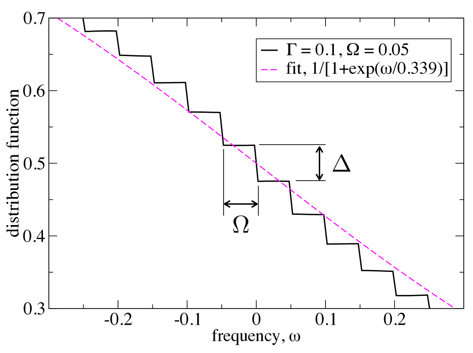
Figure 5: Fit of $f_{\rm loc}(\omega)$ at low frequency $\omega$. An analytic expression of the effective temperature $T_{\rm eff}$ is estimated from the low frequency part plotted in FIG. 3. The slope of the fit is approximated from the step $\Delta$ at $\omega=0$ as $-\Delta/\Omega$. The actual fit gives a somewhat smaller slope than the analytic estimate.

Appendix B Conductivity from linear response theory

From the Kubo formula mahan , the linear conductivity can be exactly calculated in the small $\Omega$ limit. For convenience, we calculate the current-current correlation function in the imaginary-time formalism and then analytically continue to the real-frequency in the optical conductivity pruschke . For the uniform (${\rm q}=0$) response function in the Matsubara frequency $i\nu$, the conductivity is expressed as

$$\sigma(i\nu)=\frac{i}{i\nu}\frac{1}{L\beta}\sum_{k,n}v_{k}^{2}G_{k}(i\omega_{n})G_{k}(i\omega_{n}+i\nu).$$ (48)

Here $v_{k}=2\gamma\sin(k)$ is the group velocity and the Matsubara Green’s function for the electron is given as

$$G_{k}(i\omega_{n})=\frac{1}{i\omega_{n}-\epsilon_{k}+i\Gamma(\omega_{n}/|\omega_{n}|)}=\int d\epsilon\frac{\rho_{0}(\epsilon-\epsilon_{k})}{i\omega_{n}-\epsilon},$$ (49)

with $\rho_{0}(\epsilon)=\Gamma/\pi\cdot(\epsilon^{2}+\Gamma^{2})^{-1}$. Performing the Matsubara summation and then the analytic continuation $i\nu\to\omega+i\eta$ for finite $\omega$, we have

$$\sigma(\omega) = \frac{i}{L\omega}\sum_{k}v_{k}^{2}\int d\epsilon_{1}\int d\epsilon_{2}\rho_{0}(\epsilon_{1}-\epsilon_{k})\rho_{0}(\epsilon_{2}-\epsilon_{k})$$ (50)

$$\times\frac{f(\epsilon_{1})-f(\epsilon_{2})}{\omega+\epsilon_{1}-\epsilon_{2}+i\eta}.$$

Taking its real part and the static limit $\omega\to 0$ at zero temperature, we obtain the DC linear conductivity

$$\sigma_{0} = \frac{4e^{2}a\gamma^{2}\Gamma^{2}}{\pi}\int_{0}^{2\pi}\frac{dk}{2\pi}\frac{\sin^{2}k}{(\Gamma^{2}+4\gamma^{2}\cos^{2}k)^{2}}$$ (51)

$$= \frac{2e^{2}a\gamma^{2}}{\pi\Gamma\sqrt{\Gamma^{2}+4\gamma^{2}}},$$

with the restored constants $e$ and $a$.

Appendix C Joule heating and energy flux

The current expectation value measured at the site $\ell=0$ is expressed as $\langle\hat{J}\rangle=2\gamma{\rm Im}\langle d^{\dagger}_{1}d_{0}\rangle$. Using the scattering state basis, we have

$$\langle d^{\dagger}_{1}d_{0}\rangle = \frac{g^{2}}{L}\sum_{n\alpha}[\overline{G}^{r}_{1n}(\epsilon_{\alpha}-n\Omega)]^{*}\overline{G}^{r}_{0n}(\epsilon_{\alpha}-n\Omega)f(\epsilon_{\alpha})$$

$$= \frac{\Gamma}{\pi}\sum_{nkk^{\prime}}\int_{-\infty}^{0}d\omega\frac{J_{1-k-n}J_{-k}J_{-k^{\prime}-n}J_{-k^{\prime}}}{(\omega+k\Omega-i\Gamma)(\omega+k^{\prime}\Omega+i\Gamma)}$$

$$= -\frac{\Gamma}{\pi}\sum_{k}\int_{-\infty}^{0}\frac{J_{k}J_{k-1}d\omega}{(\omega+k\Omega-i\Gamma)[\omega+(k-1)\Omega+i\Gamma]},$$

by using Eq. (25) and the Bessel function identities. We have suppressed the argument in the Bessel functions. With integration of elementary functions we obtain

$$\langle d^{\dagger}_{1}d_{0}\rangle = \frac{\Gamma}{\pi(\Omega-2i\Gamma)}\sum_{k}J_{k}\left(\frac{2\gamma}{\Omega}\right)J_{k-1}\left(\frac{2\gamma}{\Omega}\right)$$ (52)

$$\times\left[\frac{1}{2}\ln\frac{k^{2}\Omega^{2}+\Gamma^{2}}{(k-1)^{2}\Omega^{2}+\Gamma^{2}}+i\chi_{k,k-1}\right],$$

with $\chi_{nm}=\pi+\tan^{-1}\frac{n\Omega}{\Gamma}+\tan^{-1}\frac{m\Omega}{\Gamma}$. This immediately confirms that the current evaluated from the scattering state basis matches the result in Ref. fbath, .

For the operator $\langle\hat{P}\rangle$ we need to calculate $\langle(\bar{c}^{\dagger}_{1}+\bar{c}^{\dagger}_{-1})d_{0}\rangle$. The $\bar{c}^{\dagger}$-operators are expressed with the scattering state basis as

$$\bar{c}^{\dagger}_{\ell}=\frac{1}{\sqrt{L}}\sum_{\alpha}\left[\psi^{\dagger}_{\ell\alpha}+\frac{g^{2}}{L}\sum_{\ell^{\prime}\alpha^{\prime}}\frac{[\overline{G}^{r}_{\ell\ell^{\prime}}(\epsilon_{\alpha^{\prime}}-\ell^{\prime}\Omega)]^{*}\psi^{\dagger}_{\ell^{\prime}\alpha^{\prime}}}{\epsilon_{\alpha^{\prime}}-\epsilon_{\alpha}-(\ell^{\prime}-\ell)\Omega-i\eta}\right].$$ (53)

A lengthy but straightforward calculation gives

$${\rm Im}\langle(\bar{c}^{\dagger}_{1}+\bar{c}^{\dagger}_{-1})d_{0}\rangle=\frac{\Omega}{2g\gamma}\langle\hat{J}\rangle$$ (54)

which confirms the identity $\langle\hat{P}\rangle=-\Omega\langle\hat{J}\rangle$.

For the energy flux into the fermion baths, we examine

$$\langle\dot{\hat{H}}_{\rm bath}\rangle = i\langle[\hat{H}_{\rm sys},\hat{H}_{\rm bath}]\rangle$$ (55)

$$= \frac{ig}{\sqrt{L}}\sum_{\ell\alpha}(\epsilon_{\alpha}-\ell\Omega)\langle c^{\dagger}_{\ell\alpha}d_{\ell}-d^{\dagger}_{\ell}c_{\ell\alpha}\rangle.$$

First we show that $\sqrt{L^{-1}}\sum_{\alpha}\langle c^{\dagger}_{\ell\alpha}d_{\ell}-d^{\dagger}_{\ell}c_{\ell\alpha}\rangle=0$. From the steady-state condition of $\frac{d}{dt}\langle d^{\dagger}_{\ell}d_{\ell}\rangle=0$, we have $\langle[\hat{H}_{\rm Coul},d^{\dagger}_{\ell}d_{\ell}]\rangle=-\gamma\langle d^{\dagger}_{\ell+1}d_{\ell}-d^{\dagger}_{\ell}d_{\ell+1}+d^{\dagger}_{\ell-1}d_{\ell}-d^{\dagger}_{\ell}d_{\ell-1}\rangle-\frac{g}{\sqrt{L}}\sum_{\alpha}\langle c^{\dagger}_{\ell\alpha}d_{\ell}-d^{\dagger}_{\ell}c_{\ell\alpha}\rangle=0$. The first term is the total flux into the $\ell$-th site due to the current along the TB chain, and in the steady-state it is zero. Therefore we have zero particle-flux into the reservoir, $\sqrt{L^{-1}}\sum_{\alpha}\langle c^{\dagger}_{\ell\alpha}d_{\ell}-d^{\dagger}_{\ell}c_{\ell\alpha}\rangle=0$. The remaining summation $\sqrt{L^{-1}}\sum_{\alpha}\epsilon_{\alpha}\langle c^{\dagger}_{\ell\alpha}d_{\ell}-d^{\dagger}_{\ell}c_{\ell\alpha}\rangle$ is the energy flux measured with respect to the $\ell$-th reservoir chemical potential level and it should be independent of $\ell$. Setting $\ell=0$, we can rewrite the expression as follows.

Consider $G^{<}_{d\alpha}(t)=i\langle c^{\dagger}_{0\alpha}(0)d_{0}(t)\rangle$ and $G^{<}_{\alpha d}(t)=i\langle d^{\dagger}_{0}(-t)c_{0\alpha}(0)\rangle$. For the energy flux per reservoir, we can write

$$\langle\dot{\hat{h}}_{\rm bath}\rangle = \frac{g}{\sqrt{L}}\sum_{\alpha}\epsilon_{\alpha}\int[G^{<}_{d\alpha}(\omega)-G^{<}_{\alpha d}(\omega)]\frac{d\omega}{2\pi}.$$

From the Dyson’s equation meir ,

$$G^{<}_{d\alpha}(\omega)-G^{<}_{\alpha d}(\omega)$$

$$=\frac{-2\pi ig}{\sqrt{L}}\delta(\omega-\epsilon_{\alpha})\{G^{<}_{00}(\omega)-f(\omega)[G^{a}_{00}(\omega)-G^{r}_{00}(\omega)]\}$$

$$=\frac{4\pi^{2}g}{\sqrt{L}}\delta(\omega-\epsilon_{\alpha})A_{\rm loc}(\omega)[f_{\rm loc}(\omega)-f(\omega)].$$ (56)

Then

$$\langle\dot{\hat{h}}_{\rm bath}\rangle=2\Gamma\int\omega A_{\rm loc}(\omega)[f_{\rm loc}(\omega)-f(\omega)]d\omega.$$ (57)

Taking the time-derivative of the above Green’s functions at $t=0$, we have from Eq. (56),

$$\left.\frac{g}{\sqrt{L}}\sum_{\alpha}i\frac{d}{dt}\left[G^{<}_{d\alpha}(t)-G^{<}_{\alpha d}(t)\right]\right|_{t=0}$$

$$=2\Gamma\int\omega A_{\rm loc}(\omega)[f_{\rm loc}(\omega)-f(\omega)]d\omega=\langle\dot{\hat{H}}_{\rm bath}\rangle.$$

This can be equated to

$$\frac{-ig}{\sqrt{L}}\sum_{\alpha}\langle c^{\dagger}_{0\alpha}[\hat{H}_{\rm Coul},d_{0}]+[\hat{H}_{\rm Coul},d^{\dagger}_{0}]c_{0\alpha}\rangle$$ (58)

$$= -ig\gamma\langle\bar{c}^{\dagger}_{0}(d_{1}+d_{-1})-(d^{\dagger}_{1}+d^{\dagger}_{-1})\bar{c}_{0}\rangle$$

$$= -ig\gamma\langle(\bar{c}^{\dagger}_{1}+\bar{c}^{\dagger}_{-1})d_{0}-d^{\dagger}_{0}(\bar{c}_{1}+\bar{c}_{-1})\rangle,$$

where the translational invariance of the steady-state has been used. Using Eq. (54), Eq. (35) is confirmed.