Fast Exact Shortest-Path Distance Queries on Large Networks by Pruned Landmark Labeling

Abstract

We propose a new exact method for shortest-path distance queries on large-scale networks. Our method precomputes distance labels for vertices by performing a breadth-first search from every vertex. Seemingly too obvious and too inefficient at first glance, the key ingredient introduced here is pruning during breadth-first searches. While we can still answer the correct distance for any pair of vertices from the labels, it surprisingly reduces the search space and sizes of labels. Moreover, we show that we can perform 32 or 64 breadth-first searches simultaneously exploiting bitwise operations. We experimentally demonstrate that the combination of these two techniques is efficient and robust on various kinds of large-scale real-world networks. In particular, our method can handle social networks and web graphs with hundreds of millions of edges, which are two orders of magnitude larger than the limits of previous exact methods, with comparable query time to those of previous methods.

1 Introduction

A distance query asks the distance between two vertices in a graph. Without doubt, answering distance queries is one of the most fundamental operations on graphs, and it has wide range of applications. For example, on social networks, distance between two users is considered to indicate the closeness, and used in socially-sensitive search to help users to find more related users or contents [40, 42], or to analyze influential people and communities [19, 6]. On web graphs, distance between web pages is one of indicators of relevance, and used in context-aware search to give higher ranks to web pages more related to the currently visiting web page [39, 29]. Other applications of distance queries include top-$k$ keyword queries on linked data [16, 37], discovery of optimal pathways between compounds in metabolic networks [31, 32], and management of resources in computer networks [28, 7].

Of course, we can compute the distance for each query by using a breadth first search (BFS) or Dijkstra’s algorithm. However, they take more than a second for large graphs, which is too slow to use as a building block of these applications. In particular, applications such as socially-sensitive search or context-aware search should have low latency since they involve real-time interactions between users, while they need distances between a number of pairs of vertices to rank items for each search query. Therefore, distance queries should be answered much more quickly, say, microseconds.

The other extreme approach is to compute distances between all pairs of vertices beforehand and store them in an index. Though we can answer distance queries instantly, this approach is also unacceptable since preprocessing time and index size are quadratic and unrealistically large. Due to the emergence of huge graph data, design of more moderate and practical methods between these two extreme approaches has been attracting strong interest in the database community [12, 29, 41, 38, 4, 30, 17].

Generally, there are two major graph classes of real-world networks: one is road networks, and the other is complex networks such as social networks, web graphs, biological networks and computer networks. For road networks, since it is easier to grasp and exploit structures of them, research has been already very successful. Now distance queries on road networks can be processed in less than one microsecond for the complete road network of the USA [1].

In contrast, answering distance queries on complex networks is still a highly challenging problem. The methods for road networks do not perform well on these networks since structures of them are totally different. Several methods have been proposed for these networks, but they suffer from drawback of scalability. They take at least thousands of seconds or tens of thousands of seconds to index networks with millions of edges [41, 4, 2, 17].

To handle larger complex networks, apart from these exact methods, approximate methods are also studied. That is, we do not always have to answer correct distances. They are successful in terms of much better scalability and very small average relative error for random queries. However, some of these methods take milliseconds to answer queries [15, 38, 30], which is about three orders of magnitude slower than other methods. Some other methods answer queries in microseconds [29, 40], but it is reported that precision of these methods for close pairs of vertices is not high [30, 4]. This drawback might be critical for applications such as socially-sensitive search or context-aware search since, in these applications, distance queries are employed to distinguish close items.

1.1 Our Contributions

To address these issues, in this paper, we present a new method for answering distance queries in complex networks. The proposed method is an exact method. That is, it always answers exactly correct distance to queries. It has much better scalability than previous exact methods and can handle graphs with hundreds of millions of edges. Nevertheless, the query time is very small and around ten microseconds. Though our method can handle directed and/or weighted graphs as we mention later, in the following, we assume undirected, unweighted graphs for simplicity of exposition.

Our method is based on the notion of distance labeling or distance-aware 2-hop cover. The idea of 2-hop cover is as follows. For each vertex $u$, we pick up a set $C(u)$ of candidate vertices so that every pair of vertices $(u,v)$ has at least one vertex $w\in C(u)\cap C(v)$ on a shortest path between the pair. For each vertex $u$ and a vertex $w\in C(u)$, we precompute the distance $d_{G}(u,w)$ between them. We say that the set $L(u)=\{(w,d_{G}(u,w))\}_{w\in C(u)}$ is the label of $u$. Using labels, it is clear that the distance $d_{G}(u,v)$ between two vertices $u$ and $v$ can be computed as $\min\{\delta+\delta^{\prime}\mid(w,\delta)\in L(u),(w,\delta^{\prime})\in L(v)\}$. The family of labels $\{L(u)\}$ is called a 2-hop cover. Distance labeling is also commonly used in previous exact methods [13, 12, 2, 17], but we propose a totally new and different approach to compute the labels, referred to as the pruned landmark labeling.

The idea of our method is simple and rather radical: from every vertex, we conduct a breadth-first search and add the distance information to labels of visited vertices. Of course, if we naively implement this idea, we need $O(nm)$ preprocessing time and $O(n^{2})$ space to store the index, which is unacceptable. Here, $n$ is the number of vertices and $m$ is the number of edges. Our key idea to make this method practical is pruning during the breadth-first searches. Let $S$ be a set of vertices and suppose that we already have labels that can answer correct distance between two vertices if a shortest path between them passes through a vertex in $S$. Suppose we are conducting a BFS from $v$ and visiting $u$. If there is a vertex $w\in S$ such that $d_{G}(v,u)=d_{G}(v,w)+d_{G}(w,u)$, then we prune $u$. That is, we do not traverse any edges from $u$. As we prove in Section 4.3, after this pruned BFS from $v$, the labels can answer the distance between two vertices if a shortest path between them passes through a vertex in $S\cup\left\{v\right\}$.

Interestingly, our method combines the advantages of three different previous successful approaches: landmark-based approximate methods [29, 38, 30], tree-decomposition-based exact methods [41, 4], and labeling-based exact methods [13, 12, 2]. Landmark-based approximate methods achieve remarkable precision by leveraging the existence of highly central vertices in complex networks [29]. This fact is also the main reason of the power of our pruning: by conducting breadth-first searches from these central vertices first, later we can drastically prune breadth-first searches. Tree-decomposition-based methods exploit the core–fringe structure of networks [10, 27] by decomposing tree-like fringes of low tree-width. Though our method does not explicitly use tree decompositions, we prove that our method can efficiently process graphs of small tree-width. This process indicates that our method also exploits the core–fringe structure. As with other labeling-based methods, the data structure of our index is simple and query processing is very quick because of the locality of memory access.

Table 1: Summary of experimental results of previous methods and the proposed method for exact distance queries.

Method	Network	$|V|$	$|E|$	Indexing	Query
TEDI	Computer	22 K	46 K	17 s	4.2 $\mu$s
[41]	Social	0.6 M	0.6 M	2,226 s	55.0 $\mu$s
HCL	Social	7.1 K	0.1 M	1,003 s	28.2 $\mu$s
[17]	Citation	0.7 M	0.3 M	253,104 s	0.2 $\mu$s
TD	Social	0.3 M	0.4 M	9 s	0.5 $\mu$s
[4]	Social	2.4 M	4.7 M	2,473 s	0.8 $\mu$s
HHL	Computer	0.2 M	1.2 M	7,399 s	3.1 $\mu$s
[2]	Social	0.3 M	1.9 M	19,488 s	6.9 $\mu$s
	Web	0.3 M	1.5 M	4 s	0.5 $\mu$s
PLL	Social	2.4 M	4.7 M	61 s	0.6 $\mu$s
(this work)	Social	1.1 M	114 M	15,164 s	15.6 $\mu$s
	Web	7.4 M	194 M	6,068 s	4.1 $\mu$s

Though this pruned landmark labeling scheme is already powerful by itself, we propose another labeling scheme with a different kind of strength and combine them to further improve the performance. That is, we show that labeling by breadth-first search can be implemented in a bit-parallel way, which exploits the property that the number of bits $b$ in a register word is typically 32 or 64 and we can perform bit manipulations on these $b$ bits simultaneously. By this technique, we can perform BFSs from $b+1$ vertices simultaneously in $O(m)$ time. In the beginning, this bit-parallel labeling (without pruning) works better than the pruned landmark labeling since pruning does not happen much. Note that we are not talking about thread-level parallelism, and our bit-parallelism actually decreases the computational complexity by the factor of $b+1$. We can also use thread-level parallelism in addition to these two labeling schemes.

As we confirm in our experimental results, our method outperforms other state-of-the-art methods for exact distance queries. In particular, it has significantly better scalability than previous methods. It took only tens of seconds for indexing networks with millions of edges. This indexing time is two orders of magnitude faster than previous methods, which took at least thousands of seconds or even more than one day. Moreover, our method successfully handled networks with hundreds of millions of edges, which is again two orders of magnitude larger than networks that have been previously used in experiments of exact methods. The query time is also better than previous methods for networks with the same size, and we confirmed that the query time does not increase rapidly against sizes of networks. We also confirm the size of an index of our method is comparable to other methods.

In Table 1, we summarize our experimental results and those of previous exact methods presented in these papers. We listed the results for the largest two real-world complex networks from each paper. In our experiments, we further compare our method with hierarchical hub labeling [2] and the tree-decomposition-based method [4].

In Section 2, we describe related works on exact and approximate distance queries. In Section 3, we give definitions and notions used in this paper. Section 4 is devoted to explain our first scheme, the pruned landmark labeling. We explain our second scheme, the bit-parallel labeling, in Section 5. In Section 6, we mention variants of distance queries we can handle by slightly modifying our method. We explain our experimental results in Section 7, and conclude in Section 8.

2 Related Work

2.1 Exact Methods

For exact distance queries on complex networks such as social networks and web graphs, several methods are proposed recently.

Large portion of these methods can be considered as based on the idea of 2-hop cover [13]. Finding small 2-hop covers efficiently is a challenging and long-standing problem [13, 12, 2]. One of the latest methods is hierarchical hub labeling [2], which is based on a method for road networks [1]. Another latest method related to 2-hop cover is highway-centric labeling [17]. In this method, we first compute a spanning tree $T$ and use it as a “highway”. That is, when computing distance $d_{G}(u,v)$ between two vertices $u$ and $v$, we output the minimum over $d_{G}(u,w_{1})+d_{T}(w_{1},w_{2})+d_{G}(w_{2},v)$ where $w_{1}$ and $w_{2}$ are vertices in labels of $u$ and $v$, respectively, and $d_{T}(\cdot,\cdot)$ is the distance metric on the spanning tree $T$.

An approach based on tree decompositions is also reported to be efficient [41, 4]. A tree decomposition of a graph $G$ is a tree $T$ with each vertex associated with a set of vertices in $G$, called a bag [35]. Also, the set of bags containing a vertex in $G$ forms a connected component in $T$. It heuristically computes a tree decompositions and stores shortest-distance matrices for each bag. It is not hard to compute distances from this information. The smaller the size of the largest bag is, the more efficient this method is. Because of the core–fringe structure of the networks [10, 27], these networks can be decomposed into one big bag and many small bags, and the size of the largest bag is moderate though not small.

2.2 Approximate Methods

To gain more scalability than these exact methods, approximate methods, which do not always answer correct distances, also have been studied.

The major approach is the landmark-based approach [36, 40]. The basic idea of these methods is to select a subset $L$ of vertices as landmarks, and precompute the distance $d_{G}(\ell,u)$ between each landmark $\ell\in L$ and all the vertices $u\in V$. When the distance between two vertices $u$ and $v$ is queried, we answer the minimum $d_{G}(u,\ell)+d_{G}(\ell,v)$ over landmarks $\ell\in L$ as an estimate. Generally, the precision for each query depends on whether actual shortest paths pass nearby the landmarks. Therefore, by selecting central vertices as landmarks, the accuracy of estimates becomes much better than selecting landmarks randomly [29, 11]. However, for close pairs, the precision is still much worse than the average, since lengths of shortest paths between them are small and they are unlikely to pass nearby the landmarks [4].

To further improve the accuracy, several techniques were proposed [15, 38, 30]. They typically store shortest-path trees rooted at the landmarks instead of just storing distances from the landmarks. To answer queries, they extract paths from the shortest-path trees as candidates of shortest-paths, and improve them by finding loops or shortcuts. While they significantly improve the accuracy, the query time becomes up to three orders of magnitude slower.

3 Preliminaries

3.1 Notations

Table 2 lists the notations that are frequently used in this paper. In this paper, we mainly focus on networks that are modeled as graphs. Let $G=(V,E)$ be a graph with vertex set $V$ and edge set $E$. We use symbols $n$ and $m$ to denote the number of vertices $|V|$ and the number of edges $|E|$, respectively, when the graph is clear from the context. We also denote the vertex set of $G$ by $V(G)$ and the edge set of $G$ by $E(G)$. We denote the neighbors of a vertex $v\in V$ by $N_{G}(v)$. That is, $N_{G}(v)=\left\{u\in V\mid(u,v)\in E\right\}$.

Let $d_{G}(u,v)$ denote the distance between vertices $u,v$. If $u$ and $v$ are disconnected in $G$, we define $d_{G}(u,v)=\infty$. The distance in graphs is a metric, thus it satisfies the triangle inequalities. That is, for any three vertices $s$, $t$ and $v$,

$$d_{G}(s,t) \leq d_{G}(s,v)+d_{G}(v,t),$$ (1)

$$d_{G}(s,t) \geq\left|d_{G}(s,v)-d_{G}(v,t)\right|.$$ (2)

We define $P_{G}(s,t)\subseteq V$ as the set of all vertices on the shortest paths between vertices $s$ and $t$. In other words,

$$P_{G}(s,t)=\left\{v\in V\mid d_{G}(s,v)+d_{G}(v,t)=d_{G}(s,t)\right\}.$$

3.2 Problem Definition

This paper studies the following problem: given a graph $G$, construct an index to efficiently answer distance queries, which asks the distance between an arbitrary pair of vertices.

For simplicity of exposition, we mainly consider undirected, unweighted graphs. However, our algorithm can be easily extended for directed and/or weighted graphs, and we discuss about this extension in Section 6. Furthermore, our method can answer not only distances but also shortest-paths. This extension is also discussed in Section 6.

Table 2: Frequently used notations.

Notation	Description
$G=(V,E)$	A graph
$n$	Number of vertices in graph $G$
$m$	Number of edges in graph $G$
$N_{G}(v)$	Neighbors of vertex $v$ in graph $G$
$d_{G}(u,v)$	Distance between vertex $u$ and $v$ in graph $G$
$P_{G}(u,v)$	Set of all the vertices on the shortest paths
	between vertex $u$ and $v$ in graph $G$

3.3 Labels and 2-Hop Cover

The general framework of 2-hop cover [13, 12, 2], or sometimes called a labeling method, is as follows. Our method also follows this framework.

For each vertex $v$, we precompute a label denoted as $L(v)$, which is a set of pairs $(u,\delta_{uv})$, where $u$ is a vertex and $\delta_{uv}=d_{G}(u,v)$. We sometimes call the set of labels $\{L(v)\}_{v\in V}$ as an index. To answer a distance query between vertices $s$ and $t$, we compute and answer $\textsc{Query}(s,t,L)$ defined as follows,

$$\textsc{Query}(s,t,L)=$$

$$\quad\quad\min\left\{\delta_{vs}+\delta_{vt}\mid(v,\delta_{vs})\in L(s),(v,\delta_{vt})\in L(t)\right\}.$$

We define $\textsc{Query}(s,t,L)=\infty$ if $L(s)$ and $L(t)$ do not share any vertex. We call $L$ a (distance-aware) 2-hop cover of $G$ if $\textsc{Query}(s,t,L)=d_{G}(s,t)$ for any pair of vertices $s$ and $t$.

For each vertex $v$, we store the label $L(v)$ so that pairs in it are sorted by their vertices. Then, we can compute $\textsc{Query}(s,t,L)$ in $O(\left|L(s)\right|+\left|L(t)\right|)$ time using a merge-join-like algorithm.

4 Algorithm Description

4.1 Naive Landmark Labeling

We start with the following naive method. As the index, we conduct a BFS from each vertex and store distances between all pairs. Though this method is too obvious and inefficient, for the exposition of the next method, we explain the details.

Let $V=\{v_{1},v_{2},\ldots,v_{n}\}$. We start with an empty index $L_{0}$, where $L_{0}(u)=\emptyset$ for every $u\in V$. Suppose we conduct BFSs from vertices in the order of $v_{1},v_{2},\ldots,v_{n}$. After the $k$-th BFS from a vertex $v_{k}$, we add distances from $v_{k}$ to labels of reached vertices, that is, $L_{k}(u)=L_{k-1}(u)\cup\left\{(v_{k},d_{G}(v_{k},u))\right\}$ for each $u\in V$ with $d_{G}(v_{k},u)\neq\infty$. We do not change labels for unreached vertices, that is, $L_{k}(u)=L_{k-1}(u)$ for every $u\in V$ with $d_{G}(v_{k},u)=\infty$.

$L_{n}$ is the final index. Obviously $\textsc{Query}(s,t,L_{n})=d_{G}(s,t)$ for any pair of vertices $s$ and $t$, and therefore, $L_{n}$ is a correct 2-hop cover for exact distance queries. This is because, if $s$ and $t$ are reachable, then $(s,0)\in L_{n}(s)$ and $(s,d_{G}(s,t))\in L_{n}(t)$ for example.

This method can be considered as a variant of landmark-based approximate methods, which we mentioned in Section 2.2. The standard landmark-based method can be regarded as a method that precomputes $L_{l}$ instead of $L_{n}$ and estimates distance between $s$ and $t$ by $\textsc{Query}(s,t,L_{l})$, where $l\ll n$ is a parameter expressing the number of landmarks.

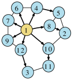
(a) First BFS from vertex 1. We visited all the vertices.

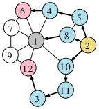
(b) Second BFS from vertex 2. We did not add labels to five vertices.

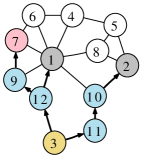
(c) Third BFS from vertex 3. We only visited the lower half of the vertices.

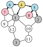
(d) Fourth BFS from vertex 4. This time we only visited the higher half.

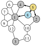
(e) Fifth BFS from vertex 5. The search space was even smaller.

Figure 1: Examples of pruned BFSs. Yellow vertices denote the roots, blue vertices denote those which we visited and labeled, red vertices denote those which we visited but pruned, and gray vertices denote those which are already used as roots.

4.2 Pruned Landmark Labeling

Then, we introduce pruning to the naive method. Similarly to the method above, we conduct pruned BFSs from vertices in the order of $v_{1},v_{2},\ldots,v_{n}$. We start with an empty index $L^{\prime}_{0}$ and create an index $L^{\prime}_{k}$ from $L^{\prime}_{k-1}$ using the information obtained by the $k$-th pruned BFS from vertex $v_{k}$.

We prune BFSs as follows. Suppose that we have an index $L^{\prime}_{k-1}$ and we are conducting a BFS from $v_{k}$ to create a new index $L^{\prime}_{k}$. Suppose that we are visiting a vertex $u$ with distance $\delta$. If $\textsc{Query}(v_{k},u,L^{\prime}_{k-1})\leq\delta$, then we prune $u$, that is, we do not add $(v_{k},\delta)$ to $L^{\prime}_{k}(u)$ (i.e. $L^{\prime}_{k}(u)=L^{\prime}_{k-1}(u)$) and we do not traverse any edge from vertex $u$. Otherwise, we set $L^{\prime}_{k}(u)=L^{\prime}_{k-1}(u)\cup\left\{(v_{k},\delta)\right\}$ and traverse all the edges from the vertex $u$ as usual. As with the previous method, we also set $L^{\prime}_{k}(u)=L^{\prime}_{k-1}(u)$ for all vertices $u\in V$ that were not visited in the $k$-th pruned BFS. This algorithm, performing pruned BFSs, is described as Algorithm 1, and the whole preprocessing algorithm is described as Algorithm 2.

Figure 1 shows examples of pruned BFSs. The first pruned BFS from vertex 1 visits all the vertices (Figure 1a). During the next pruned BFS from vertex 2 (Figure 1b), when we visit vertex 6, since $\textsc{Query}(2,6,L^{\prime}_{1})=d_{G}(2,1)+d_{G}(1,6)=3=d_{G}(2,6)$, we prune vertex 6 and we do not traverse edges from it. We also prune vertices 1 and 12. As the number of performed BFSs increases, we can confirm that the search space gets smaller and smaller (Figure 1c,1d and 1e).

Algorithm 1 Pruned BFS from $v_{k}\in V$ to create index $L^{\prime}_{k}$.

1:procedure PrunedBFS($G$, $v_{k}$, $L^{\prime}_{k-1}$)

2:     $Q\leftarrow$ a queue with only one element $v_{k}$.

3:     $P[v_{k}]\leftarrow 0$ and $P[v]\leftarrow\infty$ for all $v\in V(G)\setminus\left\{v_{k}\right\}$.

4:     $L^{\prime}_{k}[v]\leftarrow L^{\prime}_{k-1}[v]$ for all $v\in V(G)$.

5:     while $Q$ is not empty do

6:         Dequeue $u$ from $Q$.

7:         if Query($v_{k}$, $u$, $L^{\prime}_{k-1}$) $\leq P[u]$ then

8:              continue          

9:         $L^{\prime}_{k}[u]\leftarrow L^{\prime}_{k-1}[u]\cup\left\{(v_{k},P[v_{k}])\right\}$

10:         for all $w\in N_{G}(v)$ s.t. $P[w]=\infty$ do

11:              $P[w]\leftarrow P[u]+1$.

12:              Enqueue $w$ onto $Q$.               

13:     return $L^{\prime}_{k}$

Algorithm 2 Compute a 2-hop cover index by pruned BFS.

1:procedure Preprocess($G$)

2:     $L^{\prime}_{0}[v]\leftarrow\emptyset$ for all $v\in V(G)$.

3:     for $k=1,2,\ldots,n$ do

4:         $L^{\prime}_{k}\leftarrow$ PrunedBFS($G$, $v_{k}$, $L^{\prime}_{k-1}$)      

5:     return $L^{\prime}_{n}$

4.3 Proof of Correctness

In the following, we prove that this method computes a correct 2-hop cover index, that is, $\textsc{Query}(s,t,L^{\prime}_{n})=d_{G}(s,t)$ for any pair of vertices $s$ and $t$.

Theorem 4.1

For any $0\leq k\leq n$ and for any pair of vertices $s$ and $t$, $\textsc{Query}(s,t,L^{\prime}_{k})=\textsc{Query}(s,t,L_{k}).$

Proof 4.2.

We prove the theorem by mathematical induction on $k$. Since $L^{\prime}_{0}=L_{0}$, it is true for $k=0$. Now we assume it holds for $0,1,\ldots,k-1$ and prove it also holds for $k$.

Let $s,t$ be a pair of vertices. We assume these vertices are reachable in $G$, since otherwise the answer $\infty$ can be obviously obtained. Let $j$ be the smallest number such that $(v_{j},\delta_{v_{j}s})\in L_{k}(s),(v_{j},\delta_{v_{j}t})\in L_{k}(t)$ and $\delta_{v_{j}s}+\delta_{v_{j}t}=\textsc{Query}(s,t,L_{k})$. We prove that $(v_{j},\delta_{v_{j}s})$ and $(v_{j},\delta_{v_{j}t})$ are also included in $L^{\prime}_{k}(s)$ and $L^{\prime}_{k}(t)$. This immediately leads to $\textsc{Query}(s,t,L^{\prime}_{k})=\textsc{Query}(s,t,L_{k})$. Due to the symmetry between $s$ and $t$, we prove $(v_{j},\delta_{v_{j}s})\in L^{\prime}_{k}(s)$.

First, for any $i<j$, we prove by contradiction that $v_{i}\not\in P_{G}(v_{j},s)$. If we assume $v_{i}\in P_{G}(v_{j},s)$, from Inequality 1

$$\textsc{Query}(s,t,L_{k}) =d_{G}(s,v_{j})+d_{G}(v_{j},t)$$

$$=d_{G}(s,v_{i})+d_{G}(v_{i},v_{j})+d_{G}(v_{j},t)$$

$$\geq d_{G}(s,v_{i})+d_{G}(v_{i},t).$$

Since $(v_{i},d_{G}(s,v_{i}))\in L_{k}(s)$ and $(v_{i},d_{G}(t,v_{i}))\in L_{k}(t)$, this contradicts to the assumption of the minimality of $j$. Therefore, $v_{i}\not\in P_{G}(v_{j},s)$ holds for any $i<j$.

Now we prove that $(v_{j},d_{G}(v_{j},s))\in L^{\prime}_{k}(s)$. Actually, we prove a more general fact: $(v_{j},d_{G}(v_{j},u))\in L^{\prime}_{k}(u)$ for all $u\in P_{G}(v_{j},s)$. Note that $s\in P_{G}(v_{j},s)$. Suppose that we are conducting the $j$-th pruned BFS from $v_{j}$ to create $L_{j}$. Let $u\in P_{G}(v_{j},s)$. Since $P_{G}(v_{j},u)\subseteq P_{G}(v_{j},s)$ and $v_{i}\not\in P_{G}(v_{j},s)$ for any $i<j$, we have $v_{i}\not\in P_{G}(v_{j},u)$ for any $i<j$. Therefore, $\textsc{Query}(v_{j},u,L^{\prime}_{j-1})>d_{G}(v_{j},u)$ holds. Thus, we visit all vertices $u\in P_{G}(v_{j},s)$ without pruning, and it follows that $(v_{j},d_{G}(v_{j},u))\in L^{\prime}_{j}(u)\subseteq L^{\prime}_{k}(u)$.

As a corollary, our method is proved to be an exact distance querying method by instantiating the theorem with $k=n$.

Corollary 4.3.

For any pair of vertices $s$ and $t$,

$$\textsc{Query}(s,t,L^{\prime}_{n})=d_{G}(s,t).$$

4.4 Vertex Ordering Strategies

4.4.1 Motivation

In the algorithm description above, we conducted pruned BFSs from vertices in the order of $v_{1},v_{2},\ldots,v_{n}$. We can freely choose the order, and moreover it turns out that the order is crucial for the performance of this method as we will see in the experimental results presented in Section 7.3.4.

To decide the order of vertices, we should select central vertices first in the sense that many shortest paths pass through these vertices. Since we would like to prune later BFSs as much as possible, we want to cover larger part of pairs of vertices by earlier BFSs. That is, the earlier labels should offer correct distances for as many pairs of vertices as possible, and therefore the earlier vertices should be those who many shortest paths passes through.

This problem is quite similar to the problem of selecting good landmarks for landmark-based approximate methods, which is discussed well in [29]. In that problem, we also want to select good landmarks so that many shortest path passes through these vertices or nearby vertices.

4.4.2 Strategies

Based on the results on landmark-based methods [29], we propose and examine the following three strategies. In experiments, we basically use the Degree strategy, and compare them empirically in Section 7.3.4.

Random: We order vertices randomly. We use this method as a baseline to show the significance of other strategies.

Degree: We order vertices from those with higher degree. The idea behind this strategy is that vertices with higher degree have stronger connection to many other vertices and therefore many shortest paths would pass through them.

Closeness: We order vertices from those with the highest closeness centrality. Since computing exact closeness centrality for all vertices costs $O(nm)$ time, which is too expensive for large-scale networks, we approximate closeness centrality by randomly sampling a small number of vertices and computing distances from those vertices to all vertices.

4.5 Efficient Implementation

4.5.1 Preprocessing (Algorithm 1)

Index: First, in the description above, we treated $L^{\prime}_{k-1}$ and $L^{\prime}_{k}$ separately and explained as if we copy $L^{\prime}_{k-1}$ to $L^{\prime}_{k}$ for simplicity of explanation. However, this copy can be easily avoided by keeping only one index and adding labels to it after each pruned BFS.

Initialization: Another important note is to avoid $O(n)$ time initialization for each pruned BFS. The reason why this method is efficient is that the search space of pruned BFSs gets much more smaller than the whole graph. However if we spend $O(n)$ time for initialization, it would be the bottleneck. What we want to do in the initialization is to set all values in the array storing tentative distances as $\infty$ (Line 3). We can avoid $O(n)$ time initialization as follows. Before we conduct the first pruned BFS, we set all values in the array $P$ as $\infty$. (This takes $O(n)$ time but we do this only once.) Then, during each pruned BFS, we store all vertices we visited, and after each pruned BFS, we set $P[v]$ as $\infty$ for all each vertex $v$ we have visited.

Arrays: For the array storing tentative distances, it is better to use 8-bit integers. Since networks of our interest are small-world networks, 8-bit integers are enough to represent distances. Using 8-bit integers, the array fits into low-level cache memories of recent computers, resulting in the speed up by reducing cache misses.

Querying: To evaluate queries for pruning (Line 7), it is faster to use an algorithm different from the normal one since we can exploit the fact here that we issue many queries whose one endpoint is always $v_{k}$. Before starting the $k$-th pruned BFS from $v_{k}$, we prepare an array $T$ of length $n$ initialized with $\infty$ and set $T[w]=\delta_{wv_{k}}$ for all $(w,\delta_{wv_{k}})\in L^{\prime}_{k-1}(v_{k})$. To evaluate $\textsc{Query}(v_{k},u,L^{\prime}_{k-1})$, for all $(w,\delta_{wu})\in L^{\prime}_{k-1}(u)$, we compute $\delta_{wu}+T[w]$ and return the minimum. Though normal querying algorithm takes $O(\left|L^{\prime}_{k-1}(v_{k})\right|+\left|L^{\prime}_{k-1}(u)\right|)$ time, this algorithm runs in $O(\left|L^{\prime}_{k-1}(u)\right|)$ time. As Line 7 is the bottleneck of the algorithm, this technique speeds up preprocessing by about twice. Note that $T$ should be represented by 8-bit integers as the same reason described above, and $O(n)$ time initialization for array $T$ should be avoided in the same way for array $P$.

Prefetching: Unfortunately, we cannot fit the index and the adjacency lists into the cache memory for large-scale networks. However, we can manually prefetch them to reduce the cache misses, since vertices which we will access soon are in the queue. Manual prefetching speeds up preprocessing by about 20%.

Thread-Level Parallelism: As with parallel BFS algorithms [3], the pruned BFS algorithm can be also parallelized. However, for simple experimental analysis and fair comparison to previous methods, we did not parallelize our implementation in the experiments.

Sorting Labels: When applying merge-join-like algorithms to answer queries, pairs in labels need to be sorted by vertices. However, actually we do not need to sort explicitly by storing ranks of vertices instead of vertices. That is, when adding a pair $(u,\delta)$ in the $i$-th pruned BFS from vertex $u$, we add a pair $(i,\delta)$ instead. Then, since pairs are added from vertices with lower rank to those with higher rank, all the labels are automatically sorted.

4.5.2 Querying

Sentinel: We add a dummy entry, $(n,\infty)$, to the label $L(v)$ for each $v\in V$. This dummy entry ensures that we find the same vertices, $n$, in the end when scanning two labels. Thus we can avoid to separately test whether we have scanned till the end.

Arrays: For each label $L(v)$, it is faster to store the array for vertices and the array for distances separately since distances are only used when vertices match [1]. We also align arrays to cache lines.

4.6 Theoretical Properties

4.6.1 Minimality

Theorem 4.4.

Let $L^{\prime}_{n}$ be the index defined in Section 4.2. $L^{\prime}_{n}$ is minimal in the sense that, for any vertex $v$ and for any pair $(u,\delta_{uv})\in L^{\prime}_{n}(v)$, there is a pair of vertices $(s,t)$ such that, if we remove $(u,\delta_{uv})$ from $L^{\prime}_{n}(v)$, we cannot answer the correct distance between $s$ and $t$.

Proof 4.5.

Let $v_{i}\in V$ and $(v_{j},\delta_{v_{j}v_{i}})\in L^{\prime}_{n}(v_{i})$. This implies $j<i$. We show that if we remove $(v_{j},\delta_{v_{j}v_{i}})$ from $L^{\prime}_{n}(v_{i})$ then we cannot answer the correct distance between $v_{i}$ and $v_{j}$. We claim that, for any $k\neq j$, either (i) $(v_{k},\delta_{v_{k}v_{i}})\not\in L^{\prime}_{n}(v_{i})$ or $(v_{k},\delta_{v_{k}v_{j}})\not\in L^{\prime}_{n}(v_{j})$ holds, or (ii) $d_{G}(v_{i},v_{k})+d_{G}(v_{k},v_{j})>d_{G}(v_{i},v_{j})$ holds. Suppose $k<j$ and assume that (ii) does not hold. Then, (i) must hold since otherwise the $j$-th BFS should have pruned vertex $v_{i}$ and $(v_{j},\delta_{v_{j}v_{i}})\not\in L^{\prime}_{n}(v_{i})$. Suppose $k>j$ and assume that (ii) does not hold. Then, $v_{k}\in P_{G}(v_{i},v_{j})$ and therefore $(v_{j},\delta_{v_{j}v_{k}})\in L^{\prime}_{j}(v_{k})$, thus the $k$-th BFS prunes vertex $v_{j}$, leading to $(v_{k},\delta_{v_{k}v_{j}})\not\in L^{\prime}_{n}(v_{j})$.

4.6.2 Exploiting Existence of Highly Central Vertices

Then, we compare our method with landmark-based methods to show that our method also can exploit the existence of highly central vertices. We consider the standard landmark-based method [29, 40], which do not use any path heuristics. As we stated in Section 2.2, by selecting central vertices as landmarks, it attains remarkable average precision for real-world networks. From the following theorem, we can observe that our method is efficient for networks whose distance can be answered by landmark-based methods with such high precision, and our method also can exploit the existence of these central vertices.

Theorem 4.6.

If we assume that the standard landmark-based approximate method can answer correct distances to $(1-\epsilon)n^{2}$ pairs (out of $n^{2}$ pairs) using $k$ landmarks, then the pruned landmark labeling method gives an index with average label size $O(k+\epsilon n)$.

Proof 4.7 (Sketch).

After conducting pruned BFSs from the $k$ landmark vertices first, at most $\epsilon n^{2}$ pairs are added to the index in total, since we never add pairs whose distance can be answered from current labels.

4.6.3 Exploiting Small Tree-width of Fringes

Finally, we show a theoretical evidence that our method can also exploit tree-like fringes efficiently. As we mentioned in Section 2.1, methods based on tree decompositions were proposed for distance queries [41, 4]. Both of them extend methods which work efficiently for graphs of small tree-width, and they exploit low tree-width of fringes in real-world networks by tree decompositions. Interestingly, though we do not use tree decompositions explicitly, we can prove that our method can efficiently process graphs of small tree-width. Thus, our method implicitly exploits this property of real-world networks too. For definitions of tree-width and tree decompositions, see [35].

Theorem 4.8.

Let $w$ be the tree-width of $G$. There is an order of vertices with which the pruned landmark labeling method takes $O(wm\log n+w^{2}n\log^{2}n)$ time for preprocessing, stores an index with $O(wn\log n)$ space, and answers each query in $O(w\log n)$ time.

Proof 4.9 (Sketch).

The key ingredient is the centroid decomposition [18] of the tree decomposition. First we conduct pruned BFSs from all the vertices in a centroid bag. Then, later pruned BFSs never go beyond the bag. Therefore, we can consider as we divided the tree decomposition into disjoint components, each having at most half of the bags. We recursively repeat this procedure. The number of recurrences is at most $O(\log n)$. Since we add at most $w$ pairs to each vertex at each depth of recursion, the number of pairs in each label is $O(w\log n)$. At each depth of recursion, the total time consumed by pruned BFSs from the current components is $O(wm+w^{2}n\log n)$, where $O(wm)$ is the time for traversing edges and $O(w^{2}n\log n)$ is the time for pruning tests.

5 Bit-parallel Labeling

To further speed up both preprocessing and querying, we propose an optimizing method which exploits bit-level parallelism. Bit-parallel methods are those that perform different calculations on different bits in the same word to exploit the fact that computers can perform bitwise operations on a word at once. The word length is commonly 32 or 64 in computers of the day.

In the following, we denote the number of bits in a computer word as $b$ and assume bitwise operations on bit vectors of length $b$ can be done in $O(1)$ time. We propose an algorithm to conduct BFSs and compute labels from $b+1$ roots simultaneously in $O(m)$ time. Moreover, we also propose a method to answer distance queries for any pair of vertices via one of these $b+1$ vertices in $O(1)$ time.

5.1 Bit-parallel Labels

To describe the preprocessing algorithm and the querying algorithm, we first define what we store in the index.

As we explain in the next subsection, we conduct bit-parallel BFSs from a vertex $r$ and a subset of its neighbors $S_{r}\subseteq N_{G}(r)$ with size at most $b$. We define

$$S^{i}_{r}(v)=\left\{u\in S_{r}\mid d_{G}(u,v)-d_{G}(r,v)=i\right\}.$$

Since vertices in $S_{r}$ are neighbors of $r$, for any vertex $u\in S_{r}$ and any vertex $v\in V$, $\left|d_{G}(u,v)-d_{G}(r,v)\right|\leq 1$. Therefore, for each $v\in V$, $S_{r}$ can be partitioned into $S^{-1}_{r}(v),S^{0}_{r}(v)$, and $S^{+1}_{r}(v)$. That is, $S^{-1}_{r}(v)\cup S^{0}_{r}(v)\cup S^{+1}_{r}(v)=S_{r}$.

We compute bit-parallel labels and store them in the index. For each vertex $v\in V$, we precompute a bit-parallel label denoted as $L_{\textsc{BP}}(v)$. $L_{\textsc{BP}}(v)$ is a set of quadruples $(u,\delta_{uv},S^{-1}_{u}(v),S^{0}_{u}(v))$, where $u\in V$ is a vertex, $\delta_{uv}=d_{G}(u,v)$ and $S^{i}_{u}(v)\subseteq S_{u}$ is defined above. We store $S^{-1}_{u}(v)$ and $S^{0}_{u}(v)$ by bit vectors of $b$ bits. Note that $S^{+1}_{u}(v)$ can be obtained as $S_{u}\setminus(S^{-1}_{u}(v)\cup S^{0}_{u}(v))$, but actually we do not use $S^{+1}_{u}(v)$ in the querying algorithm.

In order to describe subsets of $S_{r}$ by bit vectors of $b$ bits, we assign an unique number between one and $\left|S_{r}\right|$ to each vertex in $S_{r}$, and express presence of the $i$-th vertex by setting the $i$-th bit.

5.2 Bit-parallel BFS

Algorithm 3 Bit-parallel BFS from $r\in V$ and $S_{r}\subseteq N_{G}(r)$.

1:procedure Bp-BFS($G$, $r$, $S_{r}$)

2:     $(P[v],S^{-1}_{r}[v],S^{0}_{r}[v])\leftarrow(\infty,\emptyset,\emptyset)$ for all $v\in V$

3:     $(P[r],S^{-1}_{r}[r],S^{0}_{r}[r])\leftarrow(0,\emptyset,\emptyset)$

4:     $(P[v],S^{-1}_{r}[v],S^{0}_{r}[v])\leftarrow(1,\left\{v\right\},\emptyset)$ for all $v\in S_{r}$

5:     $Q_{0},Q_{1}\leftarrow$ an empty queue

6:     Enqueue $r$ onto $Q_{0}$

7:     Enqueue $v$ onto $Q_{1}$ for all $v\in S_{r}$

8:     while $Q_{0}$ is not empty do

9:         $E_{0}\leftarrow\emptyset$ and $E_{1}\leftarrow\emptyset$

10:         while $Q_{0}$ is not empty do

11:              Dequeue $v$ from $Q_{0}$.

12:              for all $u\in N_{G}(v)$ do

13:                  if $P[u]=\infty\lor P[u]=P[v]+1$ then

14:                       $E_{1}\leftarrow E_{1}\cup\left\{(v,u)\right\}$

15:                       if $P[u]=\infty$ then

16:                           $P[u]\leftarrow P[v]+1$

17:                           Enqueue $u$ onto $Q_{1}$.                        

18:                  else if $P[u]=P[v]$ then

19:                       $E_{0}\leftarrow E_{0}\cup\left\{(v,u)\right\}$                                          

20:         for all $(v,u)\in E_{0}$ do

21:              $S^{0}_{r}[u]\leftarrow S^{0}_{r}[u]\cup S^{-1}_{r}[v]$          

22:         for all $(v,u)\in E_{1}$ do

23:              $S^{-1}_{r}[u]\leftarrow S^{-1}_{r}[u]\cup S^{-1}_{r}[v]$

24:              $S^{0}_{r}[u]\leftarrow S^{0}_{r}[u]\cup S^{0}_{r}[v]$          

25:         $Q_{0}\leftarrow Q_{1}$ and $Q_{1}\leftarrow\emptyset$      

26:     return $(P,S^{-1}_{r},S^{0}_{r})$

We once put aside the pruning discussed in Section 4.2 and we make a bit-parallel version of the naive labeling method discussed in Section 4.1. We introduce pruning later in Section 5.4.

Let $r\in V$ be a vertex and $S_{r}\subseteq N_{G}(r)$ be a subset of neighbors of $r$ with size at most $b$. We explain an algorithm to compute $d_{G}(r,v)$, $S^{-1}_{r}(v)$ and $S^{0}_{r}(v)$ for all $v\in V$ that are reachable from $\left\{r\right\}\cup S_{r}$. The algorithm is described as Algorithm 3. Basically we conduct a BFS from $r$ computing sets $S^{-1}$ and $S^{0}$.

Let $v$ be a vertex. Suppose that we have already computed $S^{-1}_{r}(w)$ for all $w$ such that $d_{G}(r,w)<d_{G}(r,v)$. We can compute $S^{-1}_{r}(v)$ as follows,

$$\left\{u\in S_{r}\mid u\in S^{-1}_{r}(w),w\in N_{G}(v),d_{G}(r,w)=d_{G}(r,v)-1\right\},$$

since if $u$ is in $S^{-1}_{r}(v)$, $d_{G}(u,v)=d_{G}(r,v)-1$ and therefore $u$ is on one of the shortest paths from $r$ to $v$. Similarly, assuming that we have already computed $S^{-1}_{r}(w)$ for all $w$ such that $d_{G}(r,w)\leq d_{G}(r,v)$ and $S^{0}_{r}(w)$ for all $w$ such that $d_{G}(r,w)<d_{G}(r,v)$, we can compute $S^{0}_{r}(v)$ as follows,

$$\left\{u\in S_{r}\mid u\in S_{r}^{0}(w),w\in N_{G}(v),d_{G}(r,w)=d_{G}(r,v)-1\right\}$$

$$\cup\left\{u\in S_{r}\mid u\in S_{r}^{-1}(w),w\in N_{G}(v),d_{G}(r,w)=d_{G}(r,v)\right\}.$$

Therefore, along with the breadth-first search, we can compute $S^{-1}_{r}$ and $S^{0}_{r}$ alternately by dynamic programming in the increasing order of distance from $r$. That is, first we compute $S^{-1}_{r}(v)$ for all $v\in V$ such that $d_{G}(r,v)=1$, next we compute $S^{0}_{r}(v)$ for all $v\in V$ such that $d_{G}(r,v)=1$, then we compute $S^{-1}_{r}(v)$ for all $v\in V$ such that $d_{G}(r,v)=2$, next we compute $S^{0}_{r}(v)$ for all $v\in V$ such that $d_{G}(r,v)=2$, and so on. Note that operations on sets can be done in $O(1)$ time by representing sets by bit vectors and using bitwise operations.

5.3 Bit-parallel Distance Querying

To process a distance query between a pair of vertices $s$ and $t$, as with normal labels, we scan bit-parallel labels $L_{\textsc{BP}}(s)$ and $L_{\textsc{BP}}(t)$. For each pair of quadruples that share the same root vertex, $(r,\delta_{rs},S^{-1}_{r}(s),S^{0}_{r}(s))\in L_{\textsc{BP}}(s)$ and $(r,\delta_{rt},S^{-1}_{r}(t),S^{0}_{r}(t))\in L_{\textsc{BP}}(t)$, from these quadruples we compute distance between $s$ and $t$ via one of vertices in $\left\{r\right\}\cup S_{r}$. That is, we compute $\delta=\min\limits_{u\in\left\{r\right\}\cup S_{r}}\left\{d_{G}(s,u)+d_{G}(u,t)\right\}$. A naive way is to compute $d_{G}(s,u)$ and $d_{G}(u,t)$ for all $u$ and take the minimum, which takes $O(\left|S_{r}\right|)$ time. However, we propose an algorithm to compute $\delta$ in $O(1)$ time by exploiting bitwise operations.

Let $\tilde{\delta}=d_{G}(s,r)+d_{G}(r,t)$. Since $\tilde{\delta}$ is an upper bound on $\delta$ and $d_{G}(s,u)\geq d_{G}(s,r)-1,d_{G}(u,t)\geq d_{G}(r,t)-1$ for all $u\in S_{r}$, $\tilde{\delta}-2\leq\delta\leq\tilde{\delta}$. Therefore, what we have to do is to judge whether the distance $\delta$ is $\tilde{\delta}-2$, $\tilde{\delta}-1$ or $\tilde{\delta}$.

This can be done as follows. If $S^{-1}_{r}(s)\cap S^{-1}_{r}(t)\not=\emptyset$, then $\delta=\tilde{\delta}-2$. Otherwise, if $S^{0}_{r}(s)\cap S^{-1}_{r}(t)\not=\emptyset$ or $S^{-1}_{r}(s)\cap S^{0}_{r}(t)\not=\emptyset$, then $\delta=\tilde{\delta}-1$, and otherwise $\delta=\tilde{\delta}$. Note that computing intersections of sets can be done by bitwise AND operations. Therefore, all these operations can be done in $O(1)$ time. Thus, the distance $\delta$ can be computed in $O(1)$ time, and, in total, we can answer each query in $O(\left|L_{\textsc{BP}}(s)\right|+\left|L_{\textsc{BP}}(t)\right|)$ time.

5.4 Introducing to Pruned Labeling

Now we discuss how to combine this bit-parallel labeling methods and the pruned labeling method discussed in Section 4.2. We propose a simple and efficient way as follows. First we conduct bit-parallel BFSs without pruning for $t$ times, where $t$ is a parameter. Then, we conduct pruned BFSs using both the bit-parallel labels and normal labels for pruning.

This method exploits different strength of the pruned labeling method and the bit-parallel labeling method. In the beginning, pruning does not work much and pruned BFSs visits large portion of the vertices. Therefore, instead of pruned labeling, we use bit-parallel labeling without pruning to efficiently cover a larger part of pairs of vertices. Skipping the overhead of vain pruning tests also contributes the speed-up.

As roots and neighbor sets for bit-parallel BFSs, we propose to greedily use vertices with the highest priority: we select a vertex with the highest priority as the root $r$ among remaining vertices, and we select up to $b$ vertices with the highest priority as the set $S_{r}$ among remaining neighbors.

As we see in the experimental results in Section 7, this method improves the preprocessing time, the index size and the query time. Moreover, as we also confirm in the experiments, if we do not set too large value as $t$, at least it does not spoil the performance. Therefore we do not have to be too serious about finding a proper value for $t$, and our method is still easy to use.

6 Variants and Extensions

Shortest-Path Queries: To answer not only distances but also shortest-paths, we store sets of tuples instead of pairs as labels. Label $L(v)$ is a set of triples $(u,\delta_{uv},p_{uv})$, where $p_{uv}\in V$ is the parent of $u$ in the pruned breadth-first search tree rooted at $u$ created by the pruned BFS from $u$. We can restore the shortest path between $v$ and $u$ by ascending the tree from $v$ to the parents.

Weighted Graphs: To treat weighted graphs, the only necessary change is to perform pruned Dijkstra’s algorithm instead of pruned BFSs. Bit-parallel labeling cannot be used for weighted graphs.

Directed Graphs: To treat directed graphs, we first redefine $d_{G}(u,v)$ as the distance from $u$ to $v$. Then, we store two labels $L_{\textsc{OUT}}(v)$ and $L_{\textsc{IN}}(v)$ for each vertex. Label $L_{\textsc{OUT}}(v)$ is a set of pairs $(u,\delta_{vu})$, where $u\in V$ and $\delta_{vu}=d_{G}(v,u)$, and Label $L_{\textsc{IN}}(v)$ is a set of pairs $(u,\delta_{uv})$, where $u\in V$ and $\delta_{uv}=d_{G}(u,v)$. We can answer the distance from vertex $s$ to vertex $t$ by $L_{\textsc{OUT}}(s)$ and $L_{\textsc{IN}}(t)$. To compute these labels, from each vertex, we conduct pruned BFSs twice: once in the forward direction and once in the reverse direction.

Disk-based Query Answering: To answer a distance query, our querying algorithm only refers to two contiguous regions. Thus, if the index is disk resident, we can answer queries with two disk seek operations, which would be still much faster than an in-memory BFS.

7 Experiments

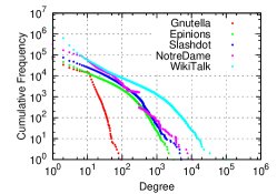
(a) Degree distribution of smaller five datasets.

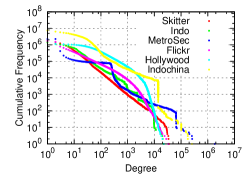
(b) Degree distribution of larger six datasets.

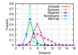
(c) Distance distribution of smaller five datasets.

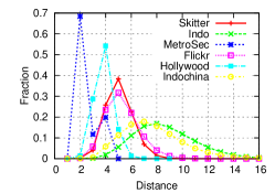
(d) Distance distribution of larger six datasets.

Figure 2: Properties of the datasets.

Table 3: Performance comparison between the proposed method and previous methods for the real-world datasets. IT denotes indexing time, IS denotes index size, QT denotes query time, and LN denotes average label size for each vertex. DNF means it did not finish in one day or ran out of memory.

Dataset	Pruned Landmark Labeling				Hierarchical Hub Labeling [2]				Tree Decomposition [4]			BFS
	IT	IS	QT	LN	IT	IS	QT	LN	IT	IS	QT
Gnutella	54 s	209 MB	5.2 $\mu$s	437+16	245 s	380 MB	11 $\mu$s	1,275	209 s	68 MB	19 $\mu$s	3.2 ms
Epinions	1.7 s	32 MB	0.5 $\mu$s	7+16	495 s	93 MB	2.2 $\mu$s	256	128 s	42 MB	11 $\mu$s	7.4 ms
Slashdot	6.0 s	48 MB	0.8 $\mu$s	14+16	670 s	182 MB	3.9 $\mu$s	464	343 s	83 MB	12 $\mu$s	12 ms
NotreDame	4.5 s	138 MB	0.5 $\mu$s	29+16	10,256 s	64 MB	0.4 $\mu$s	41	243 s	120 MB	39 $\mu$s	17 ms
WikiTalk	61 s	1.0 GB	0.6 $\mu$s	9+16	DNF	-	-	-	2,459 s	416 MB	1.8 $\mu$s	197 ms
Skitter	359 s	2.7 GB	2.3 $\mu$s	123+64	DNF	-	-	-	DNF	-	-	190 ms
Indo	173 s	2.3 GB	1.6 $\mu$s	133+64	DNF	-	-	-	DNF	-	-	150 ms
MetroSec	108 s	2.5 GB	0.7 $\mu$s	19+64	DNF	-	-	-	DNF	-	-	150 ms
Flickr	866 s	4.0 GB	2.6 $\mu$s	247+64	DNF	-	-	-	DNF	-	-	361 ms
Hollywood	15,164 s	12 GB	15.6 $\mu$s	2,098+64	DNF	-	-	-	DNF	-	-	1.2 s
Indochina	6,068 s	22 GB	4.1 $\mu$s	415+64	DNF	-	-	-	DNF	-	-	1.5 s

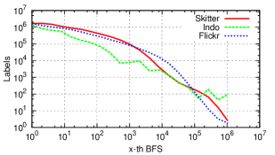
(a) Number of vertices labeled in each pruned BFS.

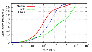
(b) Cumulative distribution of the number of vertices labeled in each pruned BFS.

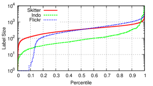
(c) Distribution of the sizes of labels.

Figure 3: Effect of pruning and sizes of labels.

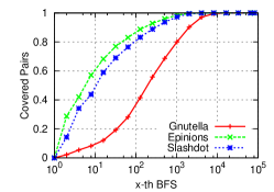
(a) Average

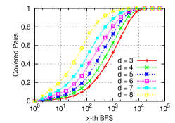
(b) Distance-wise, Gnutella

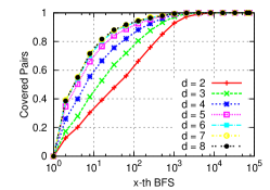
(c) Distance-wise, Epinions

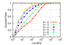
(d) Distance-wise, Slashdot

Figure 4: Fraction of pairs of vertices whose distance can be answered by index, against number of performed pruned BFS.

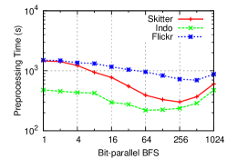
(a) Preprocessing time

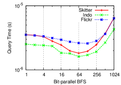
(b) Query time

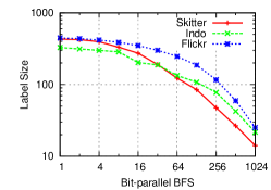
(c) Average size of a normal label

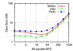
(d) Index size

Figure 5: Performance against number of bit-parallel BFSs.

We conducted experiments on a Linux server with Intel Xeon X5670 (2.93 GHz) and 48GB of main memory. The proposed method was implemented in C++. We used 8-bit integers to represent distances, 32-bit integers to represent vertices, and 64-bit integers to conduct bit-parallel BFSs. For vertex ordering, we mainly use the Degree strategy and we do not specify the vertex ordering strategy unless we use other strategies. For query time, we generally report the average time for 1,000,000 random queries.

7.1 Datasets

Table 4: Datasets

Dataset	Network	$\left|V\right|$	$\left|E\right|$
Gnutella	Computer	63 K	148 K
Epinions	Social	76 K	509 K
Slashdot	Social	82 K	948 K
Notredame	Web	326 K	1.5 M
WikiTalk	Social	2.4 M	4.7 M
Skitter	Computer	1.7 M	11 M
Indo	Web	1.4 M	17 M
MetroSec	Computer	2.3 M	22 M
Flickr	Social	1.8 M	23 M
Hollywood	Social	1.1 M	114 M
Indochina	Web	7.4 M	194 M

To show the efficiency and robustness of our method, we conducted experiments on various real-world networks: five social networks, three web graphs and three computer networks. We treated all the graphs as undirected, unweighted graphs. Basically we used five smaller datasets to compare the performance between the proposed method and previous methods and to analyze the behavior of these methods, and used larger six datasets to show the scalability of the proposed method. The types of networks, the numbers of vertices and edges are presented in Table 4.

7.1.1 Detailed Description

Gnutella: This is a graph created from a snapshot of the Gnutella P2P network in August 2002 [34].

Epinions: This graph is the on-line social network in Epinions (www.epinions.com), where each vertex represents a user and each edge represents a trust relationship [33].

Slashdot: This is the on-line social network in Slashdot (slashdot.org) obtained in February 2009. Vertices correspond to users and edges correspond to friend/foe links between the users [23].

NotreDame: This is a web graph between pages from University of Notre Dame (domain nd.edu) collected in 1999 [5].

WikiTalk: This is the on-line social network among editors of Wikipedia (www.wikipedia.org) created by communication on edits on talk pages by till January 2008 [21, 20].

Skitter: This is an Internet topology graph created from traceroutes run in 2005 by Skitter [22].

Indo: This is a web graph between pages in .in domain crawled in 2004 [9, 8].

MetroSec: This is a graph constructed from Internet traffic captured by MetroSec. Each vertex represents a computer and two vertices are linked if they appear in a packet as sender and destination [24].

Flickr: This is the on-line social network in a photo-sharing site, Flickr (www.flickr.com)[26].

Indochina: This is a web graph of web pages in the country domains of Indochina countries, crawled in 2004 [9, 8].

Hollywood: This is a social network of movie actors. Two actors are linked if they appeared in a movie together by 2009 [9, 8].

7.1.2 Statistics

First, we investigated the degree distribution of the networks, since degrees of vertices play important roles in our method when we use Degree strategy for vertex ordering. Figures 2a and 2b are the log-log plot of degree complementary cumulative distribution. As expected, we can confirm that all these networks generally exhibit power-law degree distributions.

Then, we also examined the distribution of distances. Figures 2c and 2d show distribution of distances for 1,000,000 random pairs of vertices. As we can observe from these figures, these networks are also small-world networks, in the sense that the average distance is very small.

7.2 Performance

First we present the performance of our method on the real-world datasets to show the efficiency and robustness of our method. Table 3 shows the performance of our method for the datasets. IT denotes preprocessing time, IS denotes index size, QT denotes average query time for 1,000,000 random queries, and LN denotes the average label size for each vertex, in the format of the size of normal labels (left) plus the size of bit-parallel labels (right). We set the number of times we conduct bit-parallel BFSs as 16 for first five datasets and 64 for the rest.

In Table 3, we also listed the performance of two of the state-of-the-art existing methods. One is hierarchical hub labeling [2], which is also based on distance labeling. The other one is based on tree decompositions [4], which is an improved version of TEDI [41]. For these previous methods, we used the implementations by the authors of these methods, both in C++. Experiments for hierarchical hub labeling were conducted on a Windows server with two Intel Xeon X5680 (3.33GHz) and 96GB of main memory. Experiments for the tree-decomposition-based method were conducted on our environment described above. We also described the average time to compute distance by breadth-first search for 1,000 random pairs of vertices. Among these four methods including the proposed method, only the preprocessing of hierarchical hub labeling [2] was parallelized to use all the 12 cores. All the other timing results are sequential.

7.2.1 Preprocessing Time and Scalability

Our emphasis is particularly on the large improvement in the preprocessing time, leading to much better scalability. First, we successfully preprocessed the largest two datasets Hollywood and Indochina with millions of vertices and hundreds of millions of edges in moderate preprocessing time. This is improvement of two orders of magnitude on the graph size we can handle since, as we listed in Table 1, other existing exact distance querying methods take thousands or tens of thousands of seconds to preprocess graphs with millions of edges.

For next four datasets with tens of millions of edges, it took less than one thousand seconds, while the previous methods did not finish after one day or ran out of memory. For smaller six datasets, they took at most one minute, and about at least 50 times faster than the previous methods for the most of them.

7.2.2 Query Time

The average query time was generally microseconds and at most 16 microseconds. For almost all the smaller five datasets, the query time of the proposed method is faster than the query time of the previous methods. Indeed, from Table 1, we can also observe that the query time of our method is comparable to all the existing methods for graphs of these sizes. Moreover, we can confirm that the query time does not increase much for larger networks.

7.2.3 Index Size

As for the smaller five networks, results demonstrate that our method is comparable to the previous methods with respect to index size. However, even though nowadays computers with tens of gigabytes of memory are neither rare nor expensive, reducing the index size can be an important next research issue.

7.3 Analysis

Next we analyze the behavior of our method to investigate why our method is efficient.

7.3.1 Pruned BFS

First we study how labels are computed and stored. Figure 3a shows the number of distances added to labels in each pruned BFS, and Figure 3b shows the cumulative distribution of it, that is, the ratio of the distances stored no later than each step to all the distances stored in the end. We did not use bit-parallel BFSs for these experiments.

From these figures, we can confirm the large impact of the pruning. Figure 3a shows that the number of distances added to labels in each BFS decreases so rapidly. For example, after 1,000 times of BFSs, for all the three datasets distances are added to the labels of only less than 10% of the vertices, and after conducting 10,000 times of BFSs, for all the three datasets distances are added to the labels of only less than 1% of the vertices. Figure 3b also shows that large portion of the labels are computed in the beginning.

7.3.2 Sizes of Labels

Figure 3c shows the distribution of the sizes of labels after the whole preprocessing, sorted in the ascending order of sizes. We can observe that the size of a label each vertex has do not differ much for different vertices, and few vertices have much larger labels than the average. This shows that the query time of our method is quite stable.

If you are anxious about vertices with unusually large labels, you can precompute the distance between these vertices and all the vertices and answer it directly, since the number of such vertices are few as shown in Figure 3c.

7.3.3 Pair Coverage

Figure 4a illustrates the ratio of the covered pairs of vertices, that is, the pairs of vertices whose distances can be answered correctly by current labels, at each step. We used 1,000,000 random pairs to estimate these ratios. We can observe that most pairs are covered in the beginning. This shows that such a large portion of pairs have the shortest paths that pass such a small portion of central vertices, which are selected by the Degree strategy. This is the reason why landmark-based approximate methods have good precision, and also the reason why our pruning works so effectively.

Figures 4b, 4c and 4d illustrate the ratio of the covered pairs of vertices at each step with pairs classified by distance. They show that generally distant pairs are covered earlier than close pairs. This is the reason why the precision of landmark-based approximate methods for close pairs are far worse than the precision for distant pairs. On the other hand, our method aggressively exploits this property: because distant pairs are covered in the beginning, we can prune distant vertices when processing other vertices, which results in fast preprocessing.

7.3.4 Vertex Ordering Strategies

Table 5: Average size of a label for each vertex against different vertex ordering strategies.

Dataset	Random	Degree	Closeness
Gnutella	6,171	781	865
Epinions	7,038	124	132
Slashdot	8,665	216	234
NotreDame	DNF	60	82
WikiTalk	DNF	118	158

Next we see the effect of vertex ordering strategies. Table 5 describes the average size of a label for each vertex using different vertex ordering strategies described in Section 4.4. We did not use bit-parallel BFSs for these experiments. As we can see, results are not so different between the Degree strategy and the Closeness strategy. The Degree strategy might be slightly better. On the other hand, the result of the Random strategy is much worse than other two strategies. This shows that by the Degree and Closeness strategies we can successfully capture central vertices.

7.3.5 Bit-parallel BFS

Finally, we see the effect of bit-parallel BFSs discussed in Section 5. Figure 5 shows the performance of our method against different number of times we conduct bit-parallel BFSs.

Figure 5a illustrates preprocessing time. It shows that, with a proper number of bit-parallel BFSs, preprocessing time gets two to ten times faster, resulting in the further enhancement to the scalability of our method. Figure 5b illustrates query time. We can confirm that query time also gets faster. Figure 5c shows the average size of a normal label for each vertex. As we increase the number of bit-parallel BFSs, many pairs are covered by special labels computed by bit-parallel BFSs, and the size of normal labels decreases. Figure 5d shows the index size. With a proper number of bit-parallel BFSs, index size also decreases.

Another important finding from these figures is that the performance of our method is not too sensitive to the parameter of the number of bit-parallel BFSs. As they show, the performance of our method does not become worse much unless we choose a too big number. The proper parameters seem to common between different networks. Therefore, our method still is easy to use with this bit-parallel technique.

8 Conclusions

In this paper, we proposed a novel and efficient method for exact shortest-path distance queries on large graphs. Our method is based on distance labeling to vertices, which is common to the existing exact distance querying methods, but our labeling algorithm stands on a totally new idea. Our algorithm conducts breadth-first search (BFS) from all the vertices with pruning. Though the algorithm is simple, our pruning surprisingly reduce the search space and the labels, resulting in fast preprocessing time, small index size and fast query time. Moreover, we also proposed another labeling scheme exploiting bit-level parallelism, which can be easily combined with the pruned labeling method to further improve the performance. Extensive experimental results on large-scale real-world networks of various types demonstrated the efficiency and robustness of our methods. In particular, our method can handle networks with hundreds of millions of vertices, which are two orders of magnitude larger than the limits of the previous methods, with comparable index size and query time.

We plan to investigate ways to handle even larger graphs, where indices and/or graphs might not fit in main memory. The first way is to reduce the index size by reducing graphs exploiting obvious parts and symmetry [30, 14] and compressing labels by making dictionaries of common subtrees for shortest path trees [1]. Another way is disk-based or distributed implementation. As we stated in Section 6, disk-based query answering is obvious and ready, and the challenges are particularly on preprocessing. However, since our preprocessing algorithm is a simple algorithm based on BFS, we can leverage the large body of existing work on BFS. In particular, since pruning can be done locally, the preprocessing algorithm would perform well on BSP-model-based distributed graph processing platforms [25].

9 Acknowledgments

We would like to thank Hiroshi Imai for critical reading of the manuscript, and Daniel Delling for providing us the experimental results of hierarchical hub labeling [2]. We would also like to thank the anonymous reviewers for their constructive suggestions on improving the paper. Yuichi Yoshida is supported by JSPS Grant-in-Aid for Research Activity Start-up (24800082), MEXT Grant-in-Aid for Scientific Research on Innovative Areas (24106001), and JST, ERATO, Kawarabayashi Large Graph Project.

References

- [1] I. Abraham, D. Delling, A. V. Goldberg, and R. F. Werneck. A hub-based labeling algorithm for shortest paths in road networks. In SEA, pages 230–241, 2011.
- [2] I. Abraham, D. Delling, A. V. Goldberg, and R. F. Werneck. Hierarchical hub labelings for shortest paths. In ESA, pages 24–35. 2012.
- [3] V. Agarwal, F. Petrini, D. Pasetto, and D. A. Bader. Scalable graph exploration on multicore processors. In SC, pages 1–11, 2010.
- [4] T. Akiba, C. Sommer, and K. Kawarabayashi. Shortest-path queries for complex networks: exploiting low tree-width outside the core. In EDBT, pages 144–155, 2012.
- [5] R. Albert, H. Jeong, and A. L. Barabasi. The diameter of the world wide web. Nature, 401:130–131, 1999.
- [6] L. Backstrom, D. Huttenlocher, J. Kleinberg, and X. Lan. Group formation in large social networks: membership, growth, and evolution. In KDD, pages 44–54, 2006.
- [7] S. Boccaletti, V. Latora, Y. Moreno, M. Chavez, and D. Hwang. Complex networks: Structure and dynamics. Physics reports, 424(4-5):175–308, 2006.
- [8] P. Boldi, M. Rosa, M. Santini, and S. Vigna. Layered label propagation: a multiresolution coordinate-free ordering for compressing social networks. In WWW, pages 587–596, 2011.
- [9] P. Boldi and S. Vigna. The webgraph framework I: compression techniques. In WWW, pages 595–602, 2004.
- [10] D. S. Callaway, M. E. J. Newman, S. H. Strogatz, and D. J. Watts. Network robustness and fragility: Percolation on random graphs. Physical Review Letters, 85:5468–5471, 2000.
- [11] W. Chen, C. Sommer, S.-H. Teng, and Y. Wang. A compact routing scheme and approximate distance oracle for power-law graphs. TALG, 9(1):4:1–26, 2012.
- [12] J. Cheng and J. X. Yu. On-line exact shortest distance query processing. In EDBT, pages 481–492, 2009.
- [13] E. Cohen, E. Halperin, H. Kaplan, and U. Zwick. Reachability and distance queries via 2-hop labels. In SODA, pages 937–946, 2002.
- [14] W. Fan, J. Li, X. Wang, and Y. Wu. Query preserving graph compression. In SIGMOD, pages 157–168, 2012.
- [15] A. Gubichev, S. Bedathur, S. Seufert, and G. Weikum. Fast and accurate estimation of shortest paths in large graphs. In CIKM, pages 499–508, 2010.
- [16] H. He, H. Wang, J. Yang, and P. S. Yu. Blinks: ranked keyword searches on graphs. In SIGMOD, pages 305–316, 2007.
- [17] R. Jin, N. Ruan, Y. Xiang, and V. Lee. A highway-centric labeling approach for answering distance queries on large sparse graphs. In SIGMOD, pages 445–456, 2012.
- [18] C. Jordan. Sur les assemblages de lignes. J. Reine Angew Math, 70:185–190, 1869.
- [19] D. Kempe, J. Kleinberg, and E. Tardos. Maximizing the spread of influence through a social network. In KDD, pages 137–146, 2003.
- [20] J. Leskovec, D. Huttenlocher, and J. Kleinberg. Predicting positive and negative links in online social networks. In WWW, pages 641–650, 2010.
- [21] J. Leskovec, D. Huttenlocher, and J. Kleinberg. Signed networks in social media. In CHI, pages 1361–1370, 2010.
- [22] J. Leskovec, J. Kleinberg, and C. Faloutsos. Graphs over time: Densification laws, shrinking diameters and possible explanations. In KDD, pages 177–187, 2005.
- [23] J. Leskovec, K. Lang, A. Dasgupta, and M. Mahoney. Community structure in large networks: Natural cluster sizes and the absence of large well-defined clusters. Internet Mathematics, 6(1):29–123, 2009.
- [24] C. Magnien, M. Latapy, and M. Habib. Fast computation of empirically tight bounds for the diameter of massive graphs. J. Exp. Algorithmics, 13:10:1.10–10:1.9, Feb. 2009.
- [25] G. Malewicz, M. H. Austern, A. J. Bik, J. C. Dehnert, I. Horn, N. Leiser, and G. Czajkowski. Pregel: a system for large-scale graph processing. In SIGMOD, pages 135–146, 2010.
- [26] A. Mislove, M. Marcon, K. P. Gummadi, P. Druschel, and B. Bhattacharjee. Measurement and analysis of online social networks. In IMC, pages 29–42, 2007.
- [27] M. E. J. Newman, S. H. Strogatz, and D. J. Watts. Random graphs with arbitrary degree distributions and their applications. Physical Review E, 64(2):026118 1–17, 2001.
- [28] R. Pastor-Satorras and A. Vespignani. Evolution and structure of the Internet: A statistical physics approach. Cambridge University Press, 2004.
- [29] M. Potamias, F. Bonchi, C. Castillo, and A. Gionis. Fast shortest path distance estimation in large networks. In CIKM, pages 867–876, 2009.
- [30] M. Qiao, H. Cheng, L. Chang, and J. X. Yu. Approximate shortest distance computing: A query-dependent local landmark scheme. In ICDE, pages 462–473, 2012.
- [31] S. A. Rahman, P. Advani, R. Schunk, R. Schrader, and D. Schomburg. Metabolic pathway analysis web service (pathway hunter tool at cubic). Bioinformatics, 21(7):1189–1193, 2005.
- [32] S. A. Rahman and D. Schomburg. Observing local and global properties of metabolic pathways: ‘load points’ and ‘choke points’ in the metabolic networks. Bioinformatics, 22(14):1767–1774, 2006.
- [33] M. Richardson, R. Agrawal, and P. Domingos. Trust management for the semantic web. In ISWC, volume 2870, pages 351–368. 2003.
- [34] M. Ripeanu, A. Iamnitchi, and I. Foster. Mapping the gnutella network. IEEE Internet Computing, 6(1):50–57, Jan. 2002.
- [35] N. Robertson and P. D. Seymour. Graph minors. III. Planar tree-width. J. Comb. Theory, Ser. B, 36(1):49–64, 1984.
- [36] L. Tang and M. Crovella. Virtual landmarks for the internet. In SIGCOMM, pages 143–152, 2003.
- [37] T. Tran, H. Wang, S. Rudolph, and P. Cimiano. Top-k exploration of query candidates for efficient keyword search on graph-shaped (RDF) data. In ICDE, pages 405–416, 2009.
- [38] K. Tretyakov, A. Armas-Cervantes, L. García-Bañuelos, J. Vilo, and M. Dumas. Fast fully dynamic landmark-based estimation of shortest path distances in very large graphs. In CIKM, pages 1785–1794, 2011.
- [39] A. Ukkonen, C. Castillo, D. Donato, and A. Gionis. Searching the wikipedia with contextual information. In CIKM, pages 1351–1352, 2008.
- [40] M. V. Vieira, B. M. Fonseca, R. Damazio, P. B. Golgher, D. d. C. Reis, and B. Ribeiro-Neto. Efficient search ranking in social networks. In CIKM, pages 563–572, 2007.
- [41] F. Wei. Tedi: efficient shortest path query answering on graphs. In SIGMOD, pages 99–110, 2010.
- [42] S. A. Yahia, M. Benedikt, L. V. S. Lakshmanan, and J. Stoyanovich. Efficient network aware search in collaborative tagging sites. PVLDB, 1(1):710–721, 2008.