A Method Based on Total Variation for Network Modularity Optimization using the MBO Scheme

Abstract

The study of network structure is pervasive in sociology, biology, computer science, and many other disciplines. One of the most important areas of network science is the algorithmic detection of cohesive groups of nodes called “communities”. One popular approach to find communities is to maximize a quality function known as modularity to achieve some sort of optimal clustering of nodes. In this paper, we interpret the modularity function from a novel perspective: we reformulate modularity optimization as a minimization problem of an energy functional that consists of a total variation term and an $\ell_{2}$ balance term. By employing numerical techniques from image processing and $\ell_{1}$ compressive sensing—such as convex splitting and the Merriman-Bence-Osher (MBO) scheme—we develop a variational algorithm for the minimization problem. We present our computational results using both synthetic benchmark networks and real data.

1 Introduction

Networks provide a useful representation for the investigation of complex systems, and they have accordingly attracted considerable attention in sociology, biology, computer science, and many other disciplines [48, 49]. Most of the networks that people study are graphs, which consist of nodes (i.e., vertices) to represent the elementary units of a system and edges to represent pairwise connections or interactions between the nodes.

Using networks makes it possible to examine intermediate-scale structure in complex systems. Most investigations of intermediate-scale structures have focused on community structure, in which one decomposes a network into (possibly overlapping) cohesive groups of nodes called communities [51]. There is a higher density of connections within communities than between them.

In some applications, communities have been related to functional units in networks [51]. For example, a community might be closely related to a functional module in a biological system [36] or a group of friends in a social system [59]. Because community structure in real networks can be very insightful [51, 25, 22, 49], it is useful to study algorithmic methods to detect communities. Such efforts have been useful in studies of the social organization in friendship networks [59], legislation cosponsorships in the United States Congress [61], functional modules in biology networks [27, 36], and many other situations.

To perform community detection, one needs a quantitative definition for what constitutes a community, though this relies on the goal and application one has in mind. Perhaps the most popular approach is to optimize a quality function known as modularity [44, 45, 47], and numerous computational heuristics have been developed for optimizing modularity [51, 22]. The modularity of a network partition measures the fraction of total edge weight within communities versus what one might expect if edges were placed randomly according to some null model. We give a precise definition of modularity in equation (1) in Section 2.1. Modularity gives one definition of the “quality” of a partition, and maximizing modularity is supposed to yield a reasonable partitioning of a network into disjoint communities.

Community detection is related to graph partitioning, which has been applied to problems in numerous areas (such as data clustering) [38, 57, 50]. In graph partitioning, a network is divided into disjoint sets of nodes. Graph partitioning usually requires the number of clusters to be specified to avoid trivial solutions, whereas modularity optimization does not require one to specify the number of clusters [51]. This is a desirable feature for applications such as social and biological networks.

Because modularity optimization is an NP-hard problem [7], efficient algorithms are necessary to find good locally optimal network partitions with reasonable computational costs. Numerous methods have been proposed [51, 22]. These include greedy algorithms [46, 12], extremal optimization [6, 17], simulated annealing [32, 28], spectral methods (which use eigenvectors of a modularity matrix) [47, 54], and more. The locally greedy algorithm by Blondel et al. [5] is arguably the most popular computational heuristic; it is a very fast algorithm, and it also yields high modularity values [22, 35].

In this paper, we interpret modularity optimization (using the Newman-Girvan null model [45, 49]) from a novel perspective. Inspired by the connection between graph cuts and the total variation (TV) of a graph partition, we reformulate the problem of modularity optimization as a minimization of an energy functional that consists of a graph cut (i.e., TV) term and an $\ell_{2}$ balance term. By employing numerical techniques from image processing and $\ell_{1}$ compressive sensing—such as convex splitting and the Merriman-Bence-Osher (MBO) scheme [41]—we propose a variational algorithm to perform the minimization on the new formula. We apply this method to both synthetic benchmark networks and real data sets, and we achieve performance that is competitive with the state-of-the-art modularity optimization algorithms.

The rest of this paper is organized as follows. In Section 2, we review the definition of the modularity function, and we then derive an equivalent formula of modularity optimization as a minimization problem of an energy functional that consists of a total variation term and an $\ell_{2}$ balance term. In Section 3, we explain the MBO scheme and convex splitting, which are numerical schemes that we employ to solve the minimization problem that we proposed in Section 2. In Section 4, we test our algorithms on several benchmark and real-world networks. We then review the similarity measure known as the normalized mutual information (NMI) and use it to compare network partitions with ground-truth partitions. We also evaluate the speed of our method, which we compare to classic spectral clustering [57, 38], modularity-based spectral partitioning [47, 54], and the GenLouvain code [31] (which is an implementation of a Louvain-like algorithm [5]). In Section 5, we summarize and discuss our results.

2 Method

Consider an $N$-node network, which we can represent as a weighted graph $(G,E)$ with a node set $G=\{n_{1},n_{2},\ldots,n_{N}\}$ and an edge set $E=\{w_{ij}\}_{i,j=1}^{N}$. The quantity $w_{ij}$ indicates the closeness (or similarity) of the tie between nodes $n_{i}$ and $n_{j}$, and the array of all $w_{ij}$ values forms the graph’s adjacency matrix $\textbf{W}=[w_{ij}]$. In this work, we only consider undirected networks, so $w_{ij}=w_{ji}$.

2.1 Review of the Modularity Function

The modularity of a graph partition measures the fraction of total edge weight within each community minus the edge weight that would be expected if edges were placed randomly using some null model [51]. The most common null model is the Newman-Girvan (NG) model [45], which assigns the expected edge weight between $n_{i}$ and $n_{j}$ to be $\frac{k_{i}k_{j}}{2m}$, where $k_{i}=\sum_{s=1}^{N}w_{is}$ is the strength (i.e., weighted degree) of $n_{i}$ and $2m=\sum_{i=1}^{N}k_{i}$ the total volume (i.e., total edge weight) of the graph $({G,E})$. When a network is unweighted, then $k_{i}$ is the degree of node $i$. An advantage of the NG null model is that it preserves the expected strength distribution of the network.

A partition $g=\{g_{i}\}_{i=1}^{N}$ of the graph $(G,E)$ consists of a set of disjoint subsets of the node set $G$ whose union is the entire set $G$. The quantity $g_{i}\in\{1,2,\ldots,\hat{n}\}$ is the community assignment of $n_{i}$, where there are $\hat{n}$ communities ($\hat{n}\leq N$). The modularity of the partition $g$ is defined as

$$Q(g)=\frac{1}{2m}\sum_{i,j=1}^{N}\left(w_{ij}-\gamma\frac{k_{i}k_{j}}{2m}\right)\delta(g_{i},g_{j})\,,$$ (1)

where $\gamma$ is a resolution parameter [53]. The term $\delta(g_{i},g_{j})=1$ if $g_{i}=g_{j}$ and $\delta(g_{i},g_{j})=0$ otherwise. The resolution parameter can change the scale at which a network is clustered [51, 22]. A network breaks into more communities as one increases $\gamma$.

By maximizing modularity, one expects to obtain a reasonable partioning of a network. However, this maximization problem is NP hard [7], so considerable effort has been put into the development of computational heuristics to obtain network partitions with high values of $Q$.

2.2 Reformulation of Modularity Optimization

In this subsection, we reformulate the problem of modularity optimization by deriving a new expression for $Q$ that bridges the network-science and compressive-sensing communities. This formula makes it possible to use techniques from the latter to tackle the modularity-optimization problem with low computational cost.

We start by defining the total variation (TV), weighted $\ell_{2}$-norm, and weighted mean of a function $f:G\rightarrow\mathbb{R}$:

$$|f|_{TV} :=\frac{1}{2}\sum_{i,j=1}^{N}w_{ij}\left|f_{i}-f_{j}\right|\,,$$

$$\quad\|f\|_{\ell_{2}}^{2} :=\sum_{i=1}^{N}k_{i}\left|f_{i}\right|^{2}\,,$$

$$\mathrm{mean}(f) :=\frac{1}{2m}\sum_{i=1}^{N}k_{i}f_{i}\,,$$ (2)

where $f_{i}=f(n_{i})$. The quantity $\frac{1}{2}\sum_{i,j=1}^{N}w_{ij}|f_{i}-f_{j}|$ is called the total variation because it enjoys many properties of the classical total variation $\int|\nabla f|$ of a function $f:\mathbb{R}^{n}\to\mathbb{R}$ [11]. For a vector-valued function $f=(f^{(1)},\ldots,f^{(\hat{n})})$: $G\rightarrow\mathbb{R}^{\hat{n}}$, we define

$$|f|_{TV} :=\sum_{l=1}^{\hat{n}}|f^{(l)}|_{TV}\,,$$

$$\|f\|_{\ell_{2}}^{2} :=\sum_{l=1}^{\hat{n}}\|f^{(l)}\|_{\ell_{2}}^{2}\,,$$ (3)

and $\mathrm{mean}(f):=\left(\mathrm{mean}(f^{(1)}),\ldots,\mathrm{mean}(f^{(\hat{n})})\right)$.

Given the partition $g=\{g_{i}\}_{i=1}^{N}$ defined in Section 2.1, let $A_{l}=\{n_{i}\in G,g_{i}=l\}$, where $l\in\{1,2,\ldots,\hat{n}\}$ ($\hat{n}\leq N$). Thus, $G=\cup_{l=1}^{\hat{n}}A_{l}$ is a partition of the network $(G,E)$ into disjoint communities. Note that every $A_{l}$ is allowed to be empty, so $g$ is a partition into at most $\hat{n}$ communities. Let $f^{(l)}:G\to\{0,1\}$ be the indicator function of community $l$; in other words, $f^{(l)}_{i}$ equals one if $g_{i}=l$, and it equals zero otherwise. The function $f=(f^{(1)},\ldots,f^{(\hat{n})})$ is then called the partition function (associated with $g$). Because each set $A_{l}$ is disjoint from all of the others, it is guaranteed that only a single entry of $f_{i}$ equals one for any node $i$. Therefore, $f:G\to V^{\hat{n}}\subset\mathbb{R}^{\hat{n}}$, where $V^{\hat{n}}$

$$V^{\hat{n}}:=\{(1,0,\ldots,0),(0,1,0,\ldots,0),\ldots,(0,\ldots,0,1)\}=\{\vec{e}_{l}\}_{l=1}^{\hat{n}}$$

is the standard basis of $\mathbb{R}^{\hat{n}}$.

The key observation that bridges the network-science and compressive-sensing communities is the following:

Theorem 1.

Maximizing the modularity functional $Q$ over all partitions that have at most $\hat{n}$ communities is equivalent to minimizing

$$|f|_{TV}-\gamma\|f-\mathrm{mean}(f)\|^{2}_{\ell_{2}}$$ (4)

over all functions $f:G\to V^{\hat{n}}$.

Proof.

In the language of graph partitioning, $\mathrm{vol}(A_{l}):=\sum_{n_{i}\in A_{l}}k_{i}$ denotes the volume of the set $A_{l}$, and $\mathrm{Cut}(A_{l},A_{l}^{c}):=\sum_{n_{i}\in A_{l},n_{j}\in A_{l}^{c}}w_{ij}$ is the graph cut of $A_{l}$ and $A_{l}^{c}$. Therefore,

$$Q(g) =\frac{1}{2m}\left[\big{(}2m-\sum_{g_{i}\neq g_{j}}w_{ij}\big{)}-\frac{\gamma}{2m}\sum_{l=1}^{\hat{n}}\left(\sum_{n_{i}\in A_{l},n_{j}\in A_{l}}k_{i}k_{j}\right)\right]$$

$$=1-\frac{1}{2m}\left(\sum_{l=1}^{\hat{n}}\mathrm{Cut}(A_{l},A_{l}^{c})+\frac{\gamma}{2m}\sum_{l=1}^{\hat{n}}\mathrm{vol}A_{l}^{2}\right)$$

$$=1-\gamma-\frac{1}{2m}\left(\sum_{l=1}^{\hat{n}}\mathrm{Cut}(A_{l},A_{l}^{c})-\frac{\gamma}{2m}\Big{(}\sum_{l=1}^{\hat{n}}\mathrm{vol}A_{l}\cdot\mathrm{vol}A_{l}^{c}\Big{)}\right)\,,$$ (5)

where the sum $\sum_{g_{i}\neq g_{j}}w_{ij}$ includes both $w_{ij}$ and $w_{ji}$. Note that if $\chi_{A}:G\to\{0,1\}$ is the indicator function of a subset $A\subset G$, then $\left|\chi_{A}\right|_{TV}=\mathrm{Cut}\left(A,A^{c}\right)$ and

$$\left\|\chi_{A}-\mathrm{mean}(\chi_{A})\right\|^{2}_{\ell_{2}} =\sum_{i=1}^{N}k_{i}\left|\chi_{A}(n_{i})-\frac{\mathrm{vol}(A)}{2m}\right|^{2}$$

$$=\mathrm{vol}(A)\left(1-\frac{\mathrm{vol}(A)}{2m}\right)^{2}+\mathrm{vol}\left(A^{c}\right)\left(\frac{\mathrm{vol}\left(A\right)}{2m}\right)^{2}$$

$$=\frac{\mathrm{vol}(A)\cdot\mathrm{vol}\left(A^{c}\right)}{2m}\,.$$

Because $f^{(l)}=\chi_{A_{l}}$ is the indicator function of $A_{l}$, it follows that

$$\left|f\right|_{TV}-\gamma\|f-\mathrm{mean}(f)\|^{2}_{\ell_{2}} =\sum_{l=1}^{\hat{n}}\left\{|f^{(l)}|_{TV}-\gamma\|f^{(l)}-\mathrm{mean}(f^{(l)})\|^{2}_{\ell_{2}}\right\}$$

$$=\sum_{l=1}^{\hat{n}}\left\{\mathrm{Cut}(A_{l},A_{l}^{c})-\gamma\frac{\mathrm{vol}(A_{l})\cdot\mathrm{vol}(A_{l}^{c})}{2m}\right\}\,.$$ (6)

Combining (5) and (6), we conclude that maximizing $Q$ is equivalent to minimizing (4). ∎

With the above argument, we have reformulated the problem of modularity maximization as the minimization problem (4), which corresponds to minimizing the total variation (TV) of the function $f$ along with a balance term. This yields a novel view of modularity optimization that uses the perspective of compressive sensing (see the references in [37]). In the context of compressive sensing, one seeks a solution of function $f$ that is compressible under the transform of a linear operator $\Phi$. That is, we want $\Phi f$ to be well-approximated by sparse functions. (A function is considered to be “sparse” when it is equal to or approximately equal to zero on a “large” portion of the whole domain.) Minimizing $\|\Phi f\|_{\ell^{1}}$ promotes sparsity in $\Phi f$. When $\Phi$ is the gradient operator (on a continuous domain) or the finite-differencing operator (on a discrete domain) $\nabla$, then the object $\|\Phi f\|_{\ell^{1}}=\|\nabla f\|_{\ell^{1}}$ becomes the total variation $|f|_{TV}$ [43, 37]. The minimization of TV is also common in image processing and computer vision [56, 43, 37, 10].

The expression in equation (5) is interesting because its geometric interpretation of modularity optimization contrasts with existing interpretations (e.g., probabilistic ones or in terms of the Potts model from statistical physics [47, 51]). For example, we see from (5) that finding the bipartition of the graph $G=A\cup A^{c}$ with maximal modularity is equivalent to minimizing

$$\mathrm{Cut}(A,A^{c})-\frac{\gamma}{2m}\mathrm{vol}(A)\cdot\mathrm{vol}\left(A^{c}\right)\,.$$

Note that the term $\mathrm{vol}(A)\cdot\mathrm{vol}\left(A^{c}\right)$ is maximal when $\mathrm{vol}(A)=\mathrm{vol}\left(A^{c}\right)=m$. Therefore, the second term is a balance term that favors a partition of the graph into two groups of roughly equal size. In contrast, the first term favors a partition of the graph in which few links are severed. This is reminiscent of the Balance Cut problem in which the objective is to minimize the ratio

$$\frac{\mathrm{Cut}\left(A,A^{c}\right)}{\mathrm{vol}(A)\cdot\mathrm{vol}\left(A^{c}\right)}\,.$$ (7)

In recent papers Refs. [58, 29, 30, 9, 52, 8], various TV-based algorithms were proposed to minimize ratios similar to (7).

3 Algorithm

Directly optimizing (4) over all partition functions $f:G\to V^{\hat{n}}$ is difficult due to the discrete solution space. Continuous relaxation is thus needed to simplify the optimization problem.

3.1 Ginzburg-Landau Relaxation of the Discrete Problem

Let $X^{p}$

$$X^{p}=\{f\;|\;f:G\to V^{\hat{n}}\}$$

denote the space of partition functions. Minimizing (4) over $X^{p}$ is equivalent to minimizing

$$H(f)=\begin{cases}|f|_{TV}-\gamma\|f-\mathrm{mean}(f)\|^{2}_{\ell_{2}}\,,&\text{if }f\in X^{p}\\ +\infty\,,&\text{otherwise}\end{cases}$$ (8)

over all $f:G\to\mathbb{R}^{\hat{n}}$.

The Ginzburg-Landau (GL) functional has been used as an alternative for the TV term in image processing (see the references in Ref. [4]) due to its $\Gamma$-convergence to the TV of the characteristic functions in Euclidean space [33]. Reference [4] developed a graph version of the GL functional and used it for graph-based high-dimensional data segmentation problems. The authors of Ref. [23] generalized the two-phase graphical GL functional to a multi-phase one.

For a graph $(G,E)$, the (combinatorial) graph Laplacian [11] is defined as

$$\textbf{L}=\textbf{D}-\textbf{W}\,,$$ (9)

where D is a diagonal matrix with nodes of strength $\{k_{i}\}_{i=1}^{N}$ on the diagonal and W is the weighted adjacency matrix. The operator L is linear on $\{z|z:G\to\mathbb{R}\}$, and satisfies:

$$\langle z,\textbf{L}z\rangle=\frac{1}{2}\sum_{i,j}w_{ij}(z_{i}-z_{j})^{2}\,,$$

where $z_{i}=z(n_{i})$ and $i\in\{1,2,\ldots,N\}$.

Following the idea in Refs. [4, 23], we define the Ginzburg-Landau relaxation of $H$ as follows:

$$H_{\epsilon}(f)=\frac{1}{2}\sum_{l=1}^{\hat{n}}\langle f^{(l)},\textbf{L}f^{(l)}\rangle+\frac{1}{\epsilon^{2}}\sum_{i=1}^{N}W_{\mathrm{multi}}(f_{i})-\gamma\|f-\mathrm{mean}(f)\|^{2}_{\ell_{2}}\,,$$ (10)

where $\epsilon>0$. In equation (10), $W_{\mathrm{multi}}:\mathbb{R}^{\hat{n}}\to\mathbb{R}$ is a multi-well potential (see Ref. [23]) with equal-depth wells. The minima of $W_{\mathrm{multi}}$ are spaced equidistantly, take the value $0$, and correspond to the points of $V^{\hat{n}}$. The specific formula for $W_{\mathrm{multi}}$ does not matter for the present paper, because we will discard it when we implement the MBO scheme. Note that the purpose of this multi-well term is to force $f_{i}$ to go to one of the minima, so that one obtains an approximate phase separation.

Our next theorem states that modularity optimization with an upper bound on the number of communities is well-approximated (in terms of $\Gamma$-convergence) by minimizing $H_{\epsilon}$ over all $f:G\to\mathbb{R}^{\hat{n}}$. Therefore, the discrete modularity optimization problem (4) can be approximated by a continuous optimization problem. We give the mathematical definition and relevant proofs of $\Gamma$-convergence in the Appendix.

Theorem 2 ($\Gamma$–convergence of $H_{\epsilon}$ towards $H$).

The functional $H_{\epsilon}$ $\Gamma$-converges to $H$ on the space $X=\{f\;|\;f:G\to\mathbb{R}^{\hat{n}}\}$.

Proof.

As shown in Theorem 5 (in the Appendix), $H_{\epsilon}+\gamma\|f-\mathrm{mean}(f)\|^{2}_{\ell_{2}}$ $\Gamma$-converges to $H+\gamma\|f-\mathrm{mean}(f)\|^{2}_{\ell_{2}}$ on $X$. Because $\gamma\|f-\mathrm{mean}(f)\|^{2}_{\ell_{2}}$ is continuous on the metric space $X$, it is straightforward to check that $H_{\epsilon}$ $\Gamma$-converges to $H$ according to the definition of $\Gamma$-convergence. ∎

By definition of $\Gamma$-convergence, Theorem 2 directly implies the following:

Corollary 3.

Let $f^{\epsilon}$ be the global minimizer of $H_{\epsilon}$. Any convergent subsequence of $f_{\epsilon}$ then converges to a global maximizer of the modularity $Q$ with at most $\hat{n}$ communities.

3.2 MBO Scheme, Convex splitting, and Spectral Approximation

In this subsection, we use techniques from the compressive-sensing and image-processing literatures to develop an efficient algorithm that (approximately) optimizes $H_{\epsilon}$.

In Ref. [41], an efficient algorithm (which is now called the MBO scheme) was proposed to approximate the gradient descent of the GL functional using threshold dynamics. See Refs. [2, 20, 18] for discussions of the convergence of the MBO scheme. Inspired by the MBO scheme, the authors of Ref. [19] developed a method using a PDE framework to minimize the piecewise-constant Mumford-Shah functional (introduced in Ref. [42]) for image segmentation. Their algorithm was motivated by the Chan-Vese level-set method [10] for minimizing certain variants of the Mumford-Shah functional. Note that the Chan-Vese method is related to our reformulation of modularity, because it uses the TV as a regularizer along with $\ell_{2}$ based fitting terms. The authors of Refs. [40, 23] applied the MBO scheme to graph-based problems.

The gradient-descent equation of (10) is

$$\frac{\partial f}{\partial t}=-(\mathbf{L}f^{(1)},\ldots,\mathbf{L}f^{(\hat{n})})-\frac{1}{\epsilon^{2}}\nabla W_{\mathrm{multi}}(f)+\frac{\delta}{\delta f}\left(\gamma\|f-\mathrm{mean}(f)\|^{2}_{\ell_{2}}\right)\,,$$ (11)

where $\nabla W_{\mathrm{multi}}(f):G\to\mathbb{R}^{\hat{n}}$ is the composition of the functions $\nabla W_{\mathrm{multi}}$ and $f$. Thus, one can follow the idea of the original MBO scheme to split (11) into two parts and replace the forcing part $\frac{\partial f}{\partial t}=-\frac{1}{\epsilon^{2}}\nabla W_{\mathrm{multi}}(f)$ by an associated thresholding.

We propose a Modularity MBO scheme that alternates between the following two primary steps to obtain an approximate solution $f^{n}:G\rightarrow V^{\hat{n}}$:

Step 1.

A gradient-descent process of temporal evolution consists of a diffusion term and an additional balance term:

$$\frac{\partial f}{\partial t}=-(\mathbf{L}f^{(1)},\ldots,\mathbf{L}f^{(\hat{n})})+\frac{\delta}{\delta f}\left(\gamma\|f-\mathrm{mean}(f)\|^{2}_{\ell_{2}}\right)\,.$$ (12)

We apply this process on $f^{n}$ with time $\tau_{n}$, and we repeat it for $\eta$ time steps to obtain $\hat{f}$.

Step 2.

We threshold $\hat{f}$ from $R^{\hat{n}}$ into $V^{\hat{n}}$:

$$f^{n+1}_{i}=\vec{e}_{g_{i}}\in V^{\hat{n}}\,,~{}\mathrm{where}~{}g_{i}=\mathrm{argmax}_{\{1\leq l\leq\hat{n}\}}\{\hat{f}_{i}^{(l)}\}\,.$$

This step assigns to $f_{i}^{n+1}$ the node in $V^{\hat{n}}$ that is the closest to $\hat{f}_{i}$.

To solve (12), we implement a convex-splitting scheme [21, 60]. Equation (12) is the gradient flow of the energy $H_{1}+H_{2}$, where $H_{1}(f):=\frac{1}{2}\sum_{l=1}^{\hat{n}}\langle f^{(l)},\textbf{L}f^{(l)}\rangle$ is convex and $H_{2}(f):=-\gamma\|f-\mathrm{mean}(f)\|^{2}_{\ell_{2}}$ is concave. In a discrete-time stepping scheme, the convex part is treated implicitly in the numerical scheme, whereas the concave part is treated explicitly. Note that the convex-splitting scheme for gradient-descent equations is an unconditionally stable time-stepping scheme.

The discretized time-stepping formula is

$$\frac{\hat{f}-f^{n}}{\tau_{n}} =-\frac{\delta H_{1}}{\delta f}(\hat{f})-\frac{\delta H_{2}}{\delta f}(f^{n})$$

$$=-(\mathbf{L}\hat{f}^{(1)},\ldots,\mathbf{L}\hat{f}^{(\hat{n})})+2\gamma\vec{k}\odot(f^{n}-\mathrm{mean}(f^{n}))\,,$$ (13)

where $(\vec{k}\odot f)(n_{i}):=k_{i}f_{i}$, $\hat{f}:G\rightarrow\mathbb{R}^{\hat{n}}$, ($k_{i}$ is the strength of node $n_{i}$), and $f^{n}:G\rightarrow V^{\hat{n}}$. At each step, we thus need to solve

$$\left((1+\tau_{n}\textbf{L})\hat{f}^{(1)},\ldots,(1+\tau_{n}\textbf{L})\hat{f}^{(\hat{n})}\right)=f^{n}+2\gamma\tau_{n}\vec{k}\odot\left[f^{n}-\mathrm{mean}(f^{n})\right]\,.$$ (14)

For the purpose of computational efficiency, we utilize the low-order (leading) eigenvectors (associated with the smallest eigenvalues) of the graph Laplacian $\mathbf{L}$ to approximate the operator L. The eigenvectors with higher order are more oscillatory, and resolve finer scale. Leading eigenvectors provide a set of basis to approximately represent graph functions. The more leading eigenvectors are used, the finer scales can be resolved. In the graph-clustering literature, scholars usually use a small portion of leading eigenvectors of L to find useful structural information in a graph [11, 57, 13, 3, 47], (note however that some recent work has explored the use of other eigenvectors [14]). In contrast, one typically uses much more modes when solving partial differential equations numerically (e.g., consider a psuedospectral scheme), because one needs to resolve the solution at much finer scales.

Motivated by the known utility and many successes of using leading eigenvectors (and discarding higher-order eigenvectors) in studying graph structure, we project $f$ onto the space of the $N_{\mathrm{eig}}$ leading eigenvectors to approximately solve (14). Assume that $f^{n}=\sum_{s}\phi_{s}\mathbf{a}^{n}_{s}$, $\hat{f}=\sum_{s}\phi_{s}\mathbf{\hat{a}}_{s}$, and $2\gamma\tau_{n}\vec{k}\odot(f^{n}-\mathrm{mean}(f^{n}))=\sum_{s}\phi_{s}\mathbf{b}^{n}_{s}$, where $\{\lambda_{s}\}$ are the $N_{\mathrm{eig}}$ smallest eigenvalues of the graph Laplacian L. We denote the corresponding eigenvectors (eigenfunctions) by $\{\phi_{s}\}$. Note that $\mathbf{a}^{n}_{s}$, $\mathbf{\hat{a}}_{s}$, and $\mathbf{b}^{n}_{s}$ all belong to $\mathbb{R}^{\hat{n}}$. With this representation, we obtain

$$\mathbf{\hat{a}}_{s}=\frac{\mathbf{a}^{n}_{s}+\mathbf{b}^{n}_{s}}{1+\tau_{n}\lambda_{s}}\,,\quad l\in\{1,2,\ldots,N_{\mathrm{eig}}\}$$ (15)

from (14) and are able to solve (14) more efficiently.

We summarize our Modularity MBO scheme in Algorithm 1. Note that the time complexity of each MBO iteration step is $O(N)$.

Set values for $\gamma$, $\hat{n}$, $\eta$, and $\tau_{n}=dt$.

Input $\leftarrow$ an initial function $f^{0}:G\rightarrow V^{\hat{n}}$ and the eigenvalue-eigenvector pairs $\{(\lambda_{s},\phi_{s})\}$ of the graph Laplacian L corresponding to the $N_{\mathrm{eig}}$ smallest eigenvalues.

Initialize:

$\mathbf{a}^{0}_{s}=\langle f^{0},\phi_{s}\rangle$;

$\mathbf{b}^{0}_{s}=\langle 2\gamma dt\vec{k}\odot(f^{0}-\mathrm{mean}(f^{0})),\phi_{s}\rangle$.

while $f^{n}\not=f^{n-1}$ and $n\leq 500$: do

     Diffusion:

     for $i=1\to\eta$ do

         $\mathbf{a}^{n}_{s}\leftarrow\frac{\mathbf{a}^{n}_{s}+\mathbf{b}^{n}_{s}}{1+dt\lambda_{s}}\,,~{}\mathrm{for}~{}~{}s\in\{1,2,\ldots,N_{\mathrm{eig}}\}$;

         $f^{n}\leftarrow\sum_{s}\phi_{s}\mathbf{a}^{n}_{s}$;

         $\mathbf{b}^{n}_{s}=\langle 2\gamma dt\vec{k}.*(f^{n}-\mathrm{mean}(f^{n})),\phi_{s}\rangle$;

         i=i+1;

     end for

     Thresholding:

$$f^{n+1}_{i}=\vec{e}_{g_{i}}\in V^{\hat{n}},~{}\mathrm{where}~{}g_{i}=\mathrm{argmax}_{\{1\leq l\leq\hat{n}\}}\{\hat{f}_{i}^{(l)}\}.$$

     $n=n+1;$

end while

Output $\leftarrow$ the partition function $f^{n}$.

Algorithm 1 The Modularity MBO scheme.

Unless specified otherwise, the numerical experiments in this paper using a random initial function $f^{0}$. (It takes its value in $V^{\hat{n}}$ with uniform probability by using the command rand in Matlab.)

3.3 Two Implementations of the Modularity MBO Scheme

Given an input value of the parameter $\hat{n}$, the Modularity MBO scheme partitions a graph into at most $\hat{n}$ communities. In many applications, however, the number of communities is usually not known in advance [51, 22], so it can be difficult to decide what values of $\hat{n}$ to use. Accordingly, we propose two implementations of the Modularity MBO scheme. The Recursive Modularity MBO (RMM) scheme is particularly suitable for networks that one expects a large number of communities, whereas the Multiple Input-$\hat{n}$ Modularity MBO (Multi-$\hat{n}$ MM) scheme is particularly suitable for networks that one expects to have a small number of communities.

Implementation 1. The RMM scheme performs the Modularity MBO scheme recursively, which is particular suitable for networks that one expects to have a large number of communities. In practice, we set the value of $\hat{n}$ to be large in the first round of applying the scheme, and we then let it be small for the rest of the recursion steps. In the experiments that we report in the present paper, we use $\hat{n}=50$ for the first round and $\hat{n}=\mathrm{min}(10,|S|)$ thereafter, where $|S|$ is the size of the subnetwork that one is partitioning in a given step. (We also tried $\hat{n}=10$, $20$ or $30$ for the first round and $\hat{n}=\mathrm{min}(10,|S|)$ thereafter. The results are similar.)

Importantly, the minimization problem (4) needs a slight adjustment for the recursion steps. Assume for a particular recursion step that we perform the Modularity MBO partitioning with parameter $\hat{n}$ on a network $S\subset G$ containing a subset of the nodes of the original graph. Our goal is to increase the modularity for the global network instead of the subnetwork $S$. Hence, the target energy to minimize is

$$H^{(S)}(f):=|f|^{(S)}_{TV}-\gamma\frac{m^{(S)}}{m}\left\|f-\mathrm{mean}^{(S)}(f)\right\|^{2}_{\ell_{2}}\,,$$

where $f:S\rightarrow V^{\hat{n}}\subset\mathbb{R}^{\hat{n}}$, the TV norm is $|f|^{(S)}_{TV}=\frac{1}{2}\sum_{i,j\in S}w_{ij}|f_{i}-f_{j}|_{\ell_{1}}$, the total edge weight of $S$ is $2m^{(S)}=\sum_{i\in S}k_{i}$, and $\mathrm{mean}^{(S)}(f)=\frac{1}{2m^{(S)}}\sum_{i\in S}k_{i}f_{i}$. The rest of the minimization procedures are the same as described previously.

Note that this recursive scheme is adaptive in resolving the network structure scale. The eigenvectors of the subgroups are recalculated at each recursive step, so the scales being resolved get finer as the recursion step goes. Therefore $N_{\mathrm{eig}}$ need not to be very large.

Implementation 2. For the Multi-$\hat{n}$ MM scheme, one sets a search range $T$ for $\hat{n}$, runs the Modularity MBO scheme for each $\hat{n}\in T$, and then chooses the resulting partition with the highest modularity score. It works well if one knows the approximate maximum number of communities and that number is reasonably small. One can then set the search range $T$ to be all integers between 2 and the maximum number. Even though the Multi-$\hat{n}$ MM scheme allows partitions with fewer than $\hat{n}$ clusters, it is still necessary to include small values of $\hat{n}$ in the search range to better avoid local minimums. (See the discussion of the MNIST “4-9” digits network in Section 4.2.1.) For different values of $\hat{n}$, one can reuse the previously computed eigenvectors because $\hat{n}$ does not affect the graph Laplacian. Inputting multiple choices for the random initial function $f^{0}$ (as described at the end of Section 3) also helps to reduce the chance of getting stuck in a minimum and thereby to achieve a good optimal solution for the Modularity MBO scheme. Because this initial function is used after the computation of eigenvectors, it only takes a small amount of time to rerun the MBO steps.

In Section 4, we test these two schemes on several real and synthetic networks.

4 Numerical Results

In this section, we present the numerical results of experiments that we conducted using both synthetic and real network data sets. Unless otherwise specified, our Modularity MBO schemes are all implemented in Matlab, (which are not optimized for speed). In the following tests, we set the parameters of the Modularity MBO scheme to be $\eta=5$ and $\tau_{n}=1$.

4.1 LFR Benchmark

In Ref. [34], Lancichinetti, Fortunato, and Radicchi (LFR) introduced an eponymous class of synthetic benchmark graphs to provide tougher tests of community-detection algorithms than previous synthetic benchmarks. Many real networks have heterogeneous distributions of node degree and community size, so the LFR benchmark graphs incorporate such heterogeneity. They consist of unweighted networks with a predefined set of non-overlapping communities. As described in Ref. [34], each node is assigned a degree from a power-law distribution with power $\xi$; additionally, the maximum degree is given by $k_{\mathrm{max}}$ and mean degree is $\langle k\rangle$. Community sizes in LFR graphs follow a power-law distribution with power $\beta$, subject to the constraint that the sum of the community sizes must equal the number of nodes $N$ in the network. Each node shares a fraction $1-\mu$ of its edges with nodes in its own community and a fraction $\mu$ of its edges with nodes in other communities. (The quantity $\mu$ is called the mixing parameter.) The minimum and maximum community sizes, $q_{\mathrm{min}}$ and $q_{\mathrm{max}}$, are also specified. We label the LFR benchmark data sets by $(N,\langle k\rangle,k_{\mathrm{max}},\xi,\beta,\mu,q_{\mathrm{min}},q_{\mathrm{max}})$. The code used to generate the LFR data is publicly available provided by the authors in [34].

The LFR benchmark graphs has become a popular choice for testing community detection-algorithms, and Ref. [35] uses them to test the performance of several community-detection algorithms. The authors concluded, for example, that the locally greedy Louvain algorithm [5] is one of the best performing heuristics for maximizing modularity based on the evaluation of the normalized mutual information (NMI) (discussed below in this section). Note that the time complexity of this Louvain algorithm is $O(M)$ [22], where $M$ is the number of nonzero edges in the network. In our tests, we use the GenLouvain code (in Matlab) Ref. [31], which is an implementation of a Louvain-like algorithm. The GenLouvain code a modification of the Louvain locally greedy algorithm [5], but it was not designed to be optimal for speed. We implement our RMM scheme on the LFR benchmark, and we compare our results with those of running the GenLouvain code. We use the recursive version of the Modularity MBO scheme because the LFR networks used here contain about $0.04N$ communities.

We implement the modularity-optimization algorithms on severals sets of LFR benchmark data. We then compare the resulting partitions with the known community assignments of the benchmarks (i.e., the ground truth) by examining the normalized mutual information (NMI) [15].

Normalized mutual information (NMI) is a similarity measure for comparing two partitions based on the information entropy, and it is often used for testing community-detection algorithms [34, 35]. The NMI equals 1 when two partitions are identical, and it has an expected value of $0$ when they are independent. For an $N$-node network with two partitions, $C=\{C_{1},C_{2},\ldots,C_{K}\}$ and $\hat{C}=\{\hat{C}_{1},\hat{C}_{2},\ldots,\hat{C}_{\hat{K}}\}$, that consist of non-overlapping communities, the NMI is

$$\mathrm{NMI}(C,\hat{C})=\frac{2\sum_{k=1}^{K}\sum_{\hat{k}=1}^{\hat{K}}P(k,\hat{k})\mathrm{log}\left[\frac{P(k,\hat{k})}{P(k)P(\hat{k})}\right]}{-\sum_{k=1}^{K}P(k)\mathrm{log}\left[P(k)\right]-\sum_{\hat{k}=1}^{\hat{K}}P(\hat{k})\mathrm{log}\left[P(\hat{k})\right]}\,,$$ (16)

where $P(k,\hat{k})=\frac{|C_{k}\cap\hat{C}_{\hat{k}}|}{N}$, $P(k)=\frac{|C_{k}|}{N}$, and $P(\hat{k})=\frac{|\hat{C}_{\hat{k}}|}{N}$.

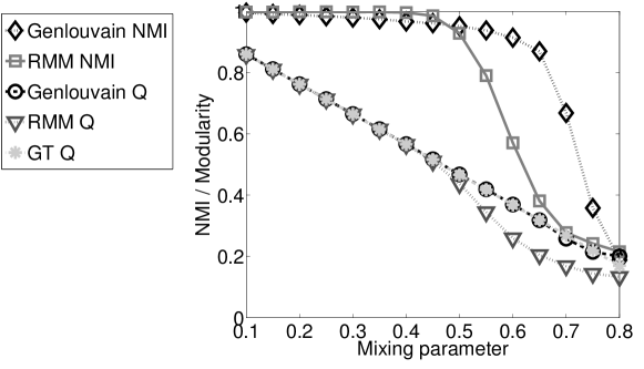
(a) NMI and Modularity ($Q$).

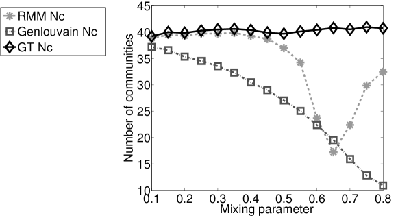
(b) Number of Communities ($N_{c}$).

Fig. 1: Tests on LFR1k networks with RMM and GenLouvain. The ground-truth communities are denoted by GT.

We examine two types of LFR networks. One is the 1000-node ensembles used in Ref. [35]:

$$\mathrm{LFR1k}:(1000,20,50,2,1,\mu,10,50)\,,$$

where $\mu\in\{0.1,0.15,\ldots,0.8\}$. The other is a 50,000-node network, which we call “LFR50k” and construct as a composition of 50 LFR1k networks. (See the detailed description below.)

4.1.1 LFR1k Networks

We use the RMM scheme (with $N_{\mathrm{eig}}=80$) and the GenLouvain code on ensembles of LFR1k$(1000,20,50,2,1,\mu,10,50)$ graphs with mixing parameters $\mu\in\{0.1,0.15,\ldots,0.8\}$. We consider 100 LFR1k networks for each value of $\mu$. The resolution parameter $\gamma$ equals one here.

In Fig. 1, we plot the mean maximized modularity score ($Q$), the number of communities ($N_{c}$), and the NMI of the partitions compared with the ground truth (GT) communities as a function of the mixing parameter $\mu$. As one can see from panel (a), the RMM scheme performs very well for $\mu<0.5$. Both its NMI score and modularity score are competitive with the results of GenLouvain. However, for $\mu\geq 0.5$, its performance drops with respect to both NMI and the modularity scores of its network partitions. From panel (b), we see that RMM tends to give partitions with more communities than GenLouvain, and this provides a better match to the ground truth. However, it is only trustworthy for $\mu<0.5$, when its NMI score is very close to $1$.

The mean computational time for one ensemble of LFR1k, which includes 15 networks corresponding to 15 values of $\mu$, is 22.7 seconds for the GenLouvain code and 17.9 seconds for the RMM scheme. As we will see later when we consider large networks, the Modularity MBO scheme scales very well in terms of its computational time.

4.1.2 LFR50k Networks

To examine the performance of our scheme on larger networks, we construct synthetic networks (LFR50k) with 50,000 nodes. To construct an LFR50k network, we start with 50 different LFR1k networks $N_{1},N_{2},\ldots,N_{50}$ with mixing parameter $\mu$, and we connect each node in $N_{s}$ ($s\in\{1,2,\ldots,50\}$) to $20\mu$ nodes in $N_{s+1}$ uniformly at random (where we note that $N_{51}=N_{1}$). We thereby obtain an LFR50k network of size $50,000$. Each community in the original $N_{s},s=1,2,\ldots,50$ is a new community in the LFR50k network. We build four such LFR50k networks for each value of $\mu=0.1,0.15,\ldots,0.8$, and we find that all such networks contain about 2000 communities. The mixing parameter of the LFR50k network constructed from LFR1k($\mu$) is approximately $\frac{2\mu}{1+\mu}$.

By construction, the LFR50k network has a similar structure as LFR1k. Importantly, simply increasing $N$ in LFR$(N,\langle k\rangle,k_{\mathrm{max}},\xi,\beta,\mu,q_{\mathrm{min}},q_{\mathrm{max}})$ to 50,000 is insufficient to preserve similarity of the network structure. A large $N$ results in more communities, so if the mixing parameter $\mu$ is held constant, then the edges of each node that are connected to nodes outside of its community will be distributed more sparsely. In another words, the mixing parameter does not entirely reflect the balance between a node’s connection within its own community versus to its connections to other communities, as there is also a dependence on the total number of communities.

The distribution of node strengths in LFR50k is scaled approximately by a factor of $(1+2\mu)$ compared to LFR1k, while the total number of edges in LFR50k is scaled approximately by a factor of $50(1+2\mu)$. Therefore, the probability null model term $\frac{k_{i}k_{j}}{2m}$ in modularity (1) is also scaled by a factor of $\frac{(1+2\mu)}{50}$. Hence, in order to probe LFR50k with a resolution scale similar to that in LFR1k, it is reasonable to use the resolution $\gamma=50$ to try to minimize issues with modularity’s resolution limit [53]. We then implement the RMM scheme ($N_{\mathrm{eig}}=100$) and the GenLouvain code. Note that we also implemented the RMM scheme with $N_{\mathrm{eig}}=500$, but there is no obvious improvement in the result even though there are about $2000$ communities. This is because the eigenvectors of the subgroups are recalculated at each recursive step, so the scales being resolved get finer as the recursion step goes.

(a) NMI and Modularity ($Q$).

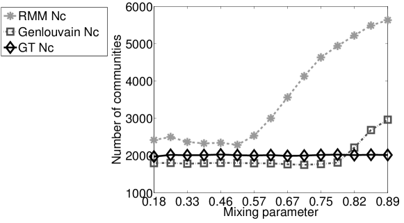
(b) Number of Communities ($N_{c}$).

Fig. 2: Tests on LFR50k data with RMM and GenLouvain.

We average the network diagnostics over the four LFR50k networks for each value of mixing parameter. In Fig. 2, we plot the network diagnostics versus the mixing parameter $\frac{2\mu}{1+\mu}$ for $\mu\in\{0.1,0.15,\ldots,0.8\}$. In panel (a), we see that the performance of RMM is good only when the mixing parameter is less than 0.5, though it is not as good as GenLouvain. It seems that the recursive Modularity MBO scheme has some difficulties in dealing with networks with very large number of clusters.

However the computational time of RMM is lower than that of the GenLouvain code [31] (though we note that it is an implementation that was not optimized for speed). The mean computational time for an ensemble of LFR50k networks, which includes 15 networks corresponding to 15 values of $\mu$, is 690 seconds for GenLouvain and 220 seconds for the RMM scheme. In Table 1, we summarize the mean computational time (in seconds) on each ensemble of LFR data.

	LFR1k	LFR50k
GenLouvain	22.7 s	690 s
RMM	17.9 s	220 s

Table 1:

4.2 MNIST Handwritten Digit Images

The MNIST database consists of 70,000 images of size $28\times 28$ pixels containing the handwritten digits “0” through “9” [62]. The digits in the images have been normalized with respect to size and centered in a fixed-size grey image. In this section, we use two networks from this database. We construct one network using all samples of the digits “4” and digit “9”, which are difficult to distinguish from each other and which constitute 13782 images of the 70000. We construct the second network using all images. In each case, our goal is to separate the distinct digits into distinct communities.

We construct the adjacency matrices (and hence the graphs) W of these two data sets as follows. First, we project each image (a $28^{2}$-dimensional datum) onto 50 principal components. For each pair of nodes $n_{i}$ and $n_{j}$ in the 50-dimensional space, we then let $w_{ij}=\exp\left(-\frac{d_{ij}^{2}}{3\sigma^{2}}\right)$ if either $n_{i}$ is among the 10 nearest neighbors of $n_{j}$ or vice versa; otherwise, we let $w_{ij}=0$. The quantity $d_{ij}$ is the $\ell_{2}$ distance between $n_{i}$ and $n_{j}$, the parameter $\sigma$ is the mean of distances between $n_{i}$ and its 10th nearest neighbor.

In this data set, the maximum number of communities is 2 when considering only the digits “4” and “9”, and it is 10 when considering all digits. We can thus choose a small search range for $\hat{n}$ and use the Multi-$\hat{n}$ Modularity MBO scheme.

4.2.1 MNIST “4-9” Digits Network

This weighted network has 13782 nodes and 194816 weighted edges. We use the labeling of each digit image as the ground truth. There are two groups of nodes: ones containing the digit “4” and ones containing the digit “9”. We use these two digits because they tend to look very similar when they are written by hand. In Fig. 3(f)(a), we show a visualization of this network, where we have projected the data projected onto the second and third leading eigenvectors of the graph Laplacian L. The difficulty of separating the “4” and “9” digits has been observed in the graph-partitioning literature (see, e.g., Ref. [30]). For example, there is a near-optimal partition of this network using traditional spectral clustering [38, 57] (see below) that splits both the “4”-group and the “9”-group roughly in half.

The modularity-optimization algorithms that we discuss for the “4-9” network use $\gamma=0.1$. We choose this resolution-parameter value so that the network is partitioned into two groups by the GenLouvain code. The question about what value of $\gamma$ to choose is beyond the scope of this paper, but it has been discussed at some length in the literature on modularity optimization [22]. Instead, we focus on evaluating the performance of our algorithm with the given value of the resolution parameter. We implement the Modularity MBO scheme with $\hat{n}=2$ and the Multi-$\hat{n}$ MM scheme, and we compare our results with that of the GenLouvain code as well as traditional spectral clustering method [38, 57].

Traditional spectral clustering is an efficient clustering method that has been used widely in computer science and applied mathematics because of its simplicity. It calculates the first $k$ nontrivial eigenvectors $\phi_{1},\phi_{2},\ldots,\phi_{k}$ (corresponding to the smallest eigenvalues) of the graph Laplacian L. Let $U\in\mathbb{R}^{N\times k}$ be the matrix containing the vectors $\phi_{1},\phi_{2},\ldots,\phi_{k}$ as columns. For $i\in\{1,2,\ldots,N\}$, let $y_{i}\in\mathbb{R}^{k}$ be the $i$th row vector of $U$. Spectral clustering then applies the $k$-means algorithm to the points $(y_{i})_{\{i=1,\ldots,N\}}$ and partitions them into $k$ groups, where $k$ is the number of clusters that was specified beforehand.

On this MNIST “4-9” digits network, we specify $k=2$ and implement spectral clustering to obtain a partition into two communities. As we show in Fig. 3(f)(b), we obtain a near-optimal solution that splits both the “4”-group and the “9”-group roughly in half. This differs markedly from the ground-truth partition in panel (a).

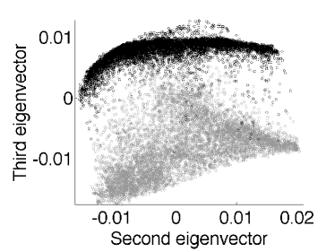
(a) Ground Truth

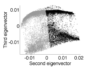
(b) Spectral Clustering with $k$-Means

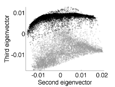
(c) Modularity MBO Scheme with $\hat{n}$=2

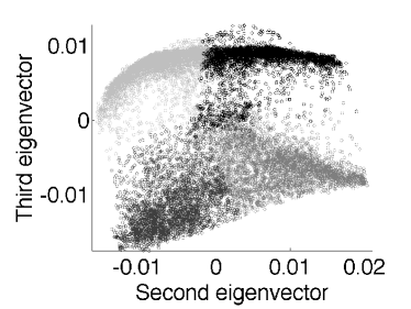
(d) Modularity MBO Scheme with $\hat{n}=8$

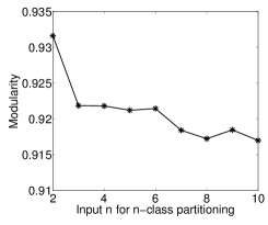
(e) Modularity Score

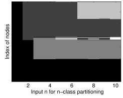
(f) Group Assignments Visualization

Fig. 3: (a)–(d) Visualization of partitions on the MNIST “4-9” digit image network by projecting it onto the second and third leading eigenvectors of the graph Laplacian. Shading indicates the community assignment. (e)–(f) Implementation results of the Multi-$\hat{n}$ Modularity MBO scheme on the MNIST “4-9” digit images. In panel (a), shading indicates the community assignment. The horizontal axis represents the input $\hat{n}$ (i.e., the maximum number of communities), and the vertical axis gives the (sorted) index of nodes. In panel (b), we plot the optimized modularity score as a function of the input $\hat{n}$.

For the Multi-$\hat{n}$ MM scheme, we use $N_{\mathrm{eig}}=80$ and the search range $\hat{n}\in\{2,3,\ldots,10\}$. We show visualizations of the partition at $\hat{n}=2$ and $\hat{n}=8$ in Figs. 3(f)(c,d). For this method, computing the spectrum of the graph Laplacian takes a significant portion of the run time (9 seconds for this data set). Importantly, however, this information can be reused for multiple $\hat{n}$, which saves time. In Fig. 3(f)(e), we show a plot of this method’s optimized modularity scores versus $\hat{n}$. Observe that the optimized modularity score achieves its maximum when we choose $\hat{n}=2$, which yields the best partition that we obtain using this method. In Fig. 3(f)(f), we show how the partition evolves as we increase the input $\hat{n}$ from 2 to 10. At $\hat{n}=2$, the network is partitioned into two groups (which agrees very well with the ground truth). For $\hat{n}>2$, however, the algorithm starts to pick out worse local optima, and either “4”-group or the “9”-group gets split roughly in half. Starting from $\hat{n}=7$, the number of communities stabilizes at about 4 instead of increasing with $\hat{n}$. This indicates that the Modularity MBO scheme allows one to obtain partitions with $N_{c}\leq\hat{n}$.

In Table 2, we show computational time and some network diagnostics for all of the resulting partitions. The modularity of the ground truth is $Q_{GT}\approx 0.9277$. Our schemes obtain high modularity and NMI scores that are comparable to those obtained using the GenLouvain code (which was not intended by its authors to be optimized for speed). The number of iterations for the Modluarity MBO scheme ranges approximately from 15 to 35 for $\hat{n}\in\{2,3,\ldots,10\}$.

	$N_{c}$	$Q$	NMI	Purity	Time (seconds)
GenLouvain	2	0.9305	0.85	0.975	110 s
Modularity MBO ($\hat{n}=2$)	2	0.9316	0.85	0.977	11 s
Multi-$\hat{n}$ MM ($\hat{n}\in\{2,3,\ldots,10\}$)	2	0.9316	0.85	0.977	25 s
Spectral Clustering ($k$-Means)	2	NA	0.003	0.534	1.5 s

Table 2:

The purity score, which we also report in Table 2, measures the extent to which a network partition matches ground truth. Suppose that an $N$-node network has a partition $C=\{C_{1},C_{2},\ldots,C_{K}\}$ into non-overlapping communities and that the ground-truth partition is $\hat{C}=\{\hat{C}_{1},\hat{C}_{2},\ldots,\hat{C}_{\hat{K}}\}$. The purity of the partition $C$ is then defined as

$$\mathrm{Prt}(C,\hat{C})=\frac{1}{N}\sum_{k=1}^{K}\mathrm{max}_{l\in\{1,\ldots,\hat{K}\}}|C_{k}\cap\hat{C}_{l}|\in[0,1]\,.$$ (17)

Intuitively, purity can by viewed as the fraction of nodes that have been assigned to the correct community. However, the purity score is not robust in estimating the performance of a partition. When the partition $C$ breaks the network into communities that consist of single nodes, then the purity score achieves a value of $1$. hence, one needs to consider other diagnostics when interpreting the purity score. In this particular data set, a high purity score does indicate good performance because the ground truth and the partitions each consist of two communities.

Observe in Table 2 that all modularity-based algorithms identified the correct community assignments for more than 97% of the nodes, whereas standard spectral clustering was only correct for just over half of the nodes. The Multi-$\hat{n}$ MM scheme takes only 25 seconds. If one specifies $\hat{n}=2$, then the Modularity MBO scheme only takes 11 seconds.

4.2.2 MNIST 70k Network

We test our new schemes further by consider the entire MNIST network of 70,000 samples containing digits from “0” to “9”. This network contains about five times as many nodes as the MNIST “4-9” network. However, the node strengths in the two networks are very similar because of how we construct the weighted adjacency matrix. We thus choose $\gamma=0.5$ so that the modularity optimization is performed at a similar resolution scale in both networks. There are 1001664 weighted edges in this network.

We implement the Multi-$\hat{n}$ MM scheme with $N_{\mathrm{eig}}=100$ and the search range $\hat{n}\in\{2,3,\ldots,20\}$. Even if $N_{c}$ is the number of communities in the true optimal solution, the input $\hat{n}=N_{c}$ might not give a partition with $N_{c}$ groups. The modularity landscape in real networks is notorious for containing a huge number of nearly degenerate local optima (especially for values of modularity $Q$ near the globally optimum value) [26], so we expect the algorithm to yield a local minimum solution rather than a global minimum. Consequently, it is preferable to extend the search range to $\hat{n}>N_{c}$, so that the larger $\hat{n}$ gives more flexibility to the algorithm to try to find the partition that optimizes modularity.

The best partition that we obtained using the search range $\hat{n}\in\{2,3,\ldots,20\}$ contains 11 communities. All of the digit groups in the ground truth except for the “1”-group are correctly matched to those communities. In the partition, the “1”-group splits into two parts, which is unsurprising given the structure of the data. In particular, the samples of the digit “1” include numerous examples that are written like a “7”. This set of samples are thus easily disconnected from the rest of “1”-group. If one considers these two parts as one community associated with “1”-group, then the partition achieves a 96% correctness in its classification of the digits.

As we illustrate in Table 3, the GenLouvain code yields comparably successful partitions as those that we obtained using the Multi-$\hat{n}$ MM scheme. By comparing the running time of the Multi-$\hat{n}$ MM scheme on both MNIST networks, one can see that our algorithm scales well in terms of speed when the network size increases. While the network size increases five times ($5\times$) and the search range gets doubled ($2\times$), the computational time increases by a factor of $11.6\approx 5\times 2$.

The number of iterations for the Modluarity MBO scheme ranges approximately from 35 to 100 for $\hat{n}\in\{2,3,\ldots,20\}$. Empirically, even though the total number of iterations can be as large as over a hundred, the modularity score quickly gets very close to its final value within the first 20 iteration.

The computational cost of the Multi-$\hat{n}$ MM scheme consists of two parts: the calculation of the eigenvectors and the MBO iteration steps. Because of the size of the MNIST 70k network, the first part costs about 90 seconds in Matlab. However, one can incorporate a faster eigenvector solver, such as the Rayleigh-Chebyshev (RC) procedure of [1], to improve the computation speed of an eigen-decomposition. This solver is especially fast for producing a small portion (in this case, ${1}/{700}$) of the leading eigenvectors for a sparse symmetric matrix. Upon implementing the RC procedure in C++ code, it only takes 12 seconds to compute the 100 leading eigenvector-eigenvalue pairs. Once the eigenvectors are calculated, they can be reused in the MBO steps for multiple values of $\hat{n}$ and different initial functions $f^{0}$. This allows good scalability, which is a particularly nice feature of using this MBO scheme.

	Nc	Q	NMI	Purity	Time (second)
GenLouvain	11	0.93	0.916	0.97	10900 s
Multi-$\hat{n}$ MM ($\hat{n}\in\{2,3,\ldots,20\}$)	11	0.93	0.893	0.96	290 s / 212 s*
Modularity MBO 3% GT ($\hat{n}=10$)	10	0.92	0.95	0.96	94.5 s / 16.5 s*

^∗Calculated with the RC procedure.

Table 3:

Another benefit of the Modularity MBO scheme is that it allows the possibility of incorporating a small portion of the ground truth in the modularity optimization process. In the present paper, we implement the Modularity MBO using 3% of the ground truth by specifying the true community assignments of 2100 nodes, which we chose uniformly at random in the initial function $f^{0}$. We also let $\hat{n}=10$. With the eigenvectors already computed (which took 12 seconds using the RC process), the MBO steps take a subsequent 4.5 seconds to yield a partition with exactly 10 communities and 96.4% of the nodes classified into the correct groups. The authors of Ref. [23] also implemented a segmentation algorithm on this MNIST 70k data with 3% of the ground truth, and they obtained a partition with a correctness 96.9% in 15.4 seconds. In their algorithm, the ground truth was enforced by adding a quadratic fidelity term to the energy functional (semi-supervised). The fidelity term is the $\ell_{2}$ distance of the unknown function $f$ and the given ground truth. In our scheme, however, it is only used in the initial function $f^{0}$. Nevertheless, it is also possible to add a fidelity term to the Modularity MBO scheme and thereby perform semi-supervised clustering.

4.3 Network-Science Coauthorships

Another well-known graph in the community detection literature is the network of coauthorships of network scientists. This benchmark was compiled by Mark Newman and first used in Ref. [47].

In the present paper, we use the graph’s largest connected component, which consists of 379 nodes representing authors and 914 weighted edges that indicate coauthored papers. We do not have any so-called ground truth for this network, but it is useful to compare partitions obtained from our algorithm with those obtained using more established algorithms. In this section, we use GenLouvain’s result as this pseudo-ground truth. In addition to Modularity-MBO, RMM, and GenLouvain, we also consider the results of modularity-based spectral partitioning methods that allow the option of either bipartitioning or tripartitioning at each recursive stage [47, 54]..

In Ref. [47], Newman proposed a spectral partitioning scheme for modularity optimization by using the leading eigenvectors (associated with the largest eigenvalues) of a so-called modularity matrix $\textbf{B}=\textbf{W}-\textbf{P}$ to approximate the modularity function $Q$. In the modularity matrix, P is the probability null model and $P_{ij}=\frac{k_{i}k_{j}}{2m}$ is the NG null model with $\gamma=1$. Assume that one uses the first $p$ leading eigenvectors $\{\textbf{u}_{1},\textbf{u}_{2},\ldots,\textbf{u}_{p}\}$, and let $\beta_{j}$ denote the eigenvalue of $\textbf{u}_{j}$ and $\textbf{U}=(\textbf{u}_{1}|\textbf{u}_{2}|\ldots|\textbf{u}_{p})$. We then define $N$ node vectors $\textbf{r}_{i}\in\mathbb{R}^{p}$ whose $j$th component is

$$(\textbf{r}_{i})_{j}=\sqrt{\beta_{j}-\alpha}U_{ij}\,,$$

where $\alpha\leq\beta_{p}$ and $j\in\{1,2,\ldots,p\}$. The modularity $Q$ is therefore approximated as

$$Q\simeq\hat{Q}=N\alpha+\sum_{l=1}^{\hat{n}}\|\textbf{R}_{l}\|_{\ell_{2}}^{2}\,,$$ (18)

where $\textbf{R}_{l}=\sum_{g_{i}=l}\textbf{r}_{i}$ is sum of all node vectors in the $l$th community (where $l\in\{1,2,\ldots,\hat{n}\}$).

A partition that maximize (18) in a given step must satisfy the geometric constraints $\textbf{R}_{l}\cdot\textbf{r}_{i}>0$, $g_{i}=l$, and $\textbf{R}_{l}\cdot\textbf{R}_{h}<0$ for all $l,h\in\{1,2,\ldots,\hat{n}\}$. Hence, if one constructs an approximation $\hat{Q}$ using $p$ eigenvectors, a network component can be split into at most $p+1$ groups in a given recursive step. The choice $p=2$ allows either bipartitioning or tripartitioning in each recursive step. Reference [47] discussed the case of general $p$ but reported results for recursive bipartitioning with $p=1$. Reference [54] implemented this spectral method with $p=2$ and a choice of bipartitioning or tripartioning at each recursive step.

In Table 4, we report diagnostics for partitions obtained by several algorithms (for $\gamma=1$). For the recursive spectral bipartitioning and tripartitioning, we use Matlab code that has been provided by the authors of Ref. [54]. They informed us that this particular implementation was not optimized for speed, so we expect it to be slow. One can create much faster implementations of the same spectral method. The utility of this method for the present comparison is that Ref. [54] includes a detailed discussion of its application to the network of network scientists. Each partitioning step in this spectral scheme either bipartitions or tripartitions a group of nodes. Moreover, as discussed in Ref. [54], a single step of the spectral tripartitioning is by itself interesting. Hence, we specify $\hat{n}=3$ for the Modularity MBO scheme as a comparison.

	$N_{c}$	Q	NMI	Purity	Time (seconds)
GenLouvain	19	0.8500	1	1	0.5 s
Spectral Recursion	39	0.8032	0.8935	0.9525	60 s
RMM	23	0.8344	0.9169	0.9367	0.8 s
Tripartition	3	0.5928	0.3993	0.8470	50 s
Modularity MBO	3	0.6165	0.5430	0.9974	0.4 s

Table 4:

From Table 4, we see that the Modularity MBO scheme with $\hat{n}=3$ gives a higher modularity than a single tripartition, and the former’s NMI and purity are both significantly higher. When we do not specify the number of clusters, the RMM scheme achieves a higher modularity score and NMI than recursive bipartitioning/tripartitioning, though the former’s purity is lower (which is not surprising due to its larger $N_{c}$). The RMM scheme and GenLouvain have similar run times. For any of these methods, one can of course use subsequent post-processing, such as Kernighan-Lin node-swapping steps [47, 54, 51], to find higher-modularity partitions.

5 Conclusion and Discussion

In summary, we have presented a novel perspective on the problem of modularity optimization by reformulating it as a minimization of an energy functional involving the total variation on a graph. This provides an interesting bridge between the network science and compressive sensing communities, and it allows the use of techniques from compressive sensing and image processing to tackle modularity optimization. In this paper, we have proposed MBO schemes that can handle large data at very low computational cost. Our algorithms produce competitive results compared to existing methods, and they scale well in terms of speed for certain networks (such as the MNIST data). In our algorithms, after computing the eigenvectors of the graph Laplacian, the time complexity of each MBO iteration step is $O(N)$.

One major part of our schemes is to calculate the leading eigenvector-eigenvalue pairs, so one can benefit from the fast numerical Rayleigh-Chebyshev procedure in Ref. [1] when dealing with large, sparse networks. Furthermore, for a given network (which is represented by a weighted adjacency matrix), one can reuse previously computed eigen-decompositions for different choices of initial functions, different values of $\hat{n}$, and different values of the resolution parameter $\gamma$. This provides welcome flexibility, and it can be used to significantly reduce computation time because the MBO step is extremely fast, as each step is $O(N)$ and the number of iterations is empirically small.

Importantly, our reformulation of modularity also provides the possibility to incorporate partial ground truth. This can accomplished either by feeding the information into the initial function or by adding a fidelity term into the functional. (We only pursued the former approach in this paper.) It is not obvious how to incorporate partial ground truth using previous optimization methods. This ability to use our method either for unsupervised or for semi-supervised clustering is a significant boon.

Appendix

The notion of $\Gamma$-convergence of functionals is now commonly used for minimization problems. See Ref. [39] for detailed introduction. In this appendix, we briefly review the definition of $\Gamma$-convergence and then prove the claim that the graphical multi-phase Ginzburg-Landau functional $\Gamma$-converges to the graph TV. This proof is a straightforward extension of the work in Ref. [24] for the two-phase graph GL functional.

Definition 4.

Let $X$ be a metric space and let $\left\{F_{n}:X\rightarrow\mathbb{R}\cup\{\pm\infty\}\right\}^{\infty}_{n=1}$ be a sequence of functionals. The sequence $F_{n}$ $\Gamma$-converges to the functional $F:X\rightarrow R\cup\{\pm\infty\}$ if, for all $f\in X$, the following lower and upper bound conditions hold:

(lower bound condition)

for every sequence $\{f_{n}\}_{n=1}^{\infty}$ such that $f_{n}\rightarrow f$, we have

$$F(f)\leq\liminf_{n\rightarrow\infty}F_{n}(f_{n})\,;$$

(upper bound condition)

there exists a sequence $\{f_{n}\}_{n=1}^{\infty}$ such that

$$F(f)\geq\limsup_{n\rightarrow\infty}F_{n}(f_{n})\,.$$

Reference [23] proposed the following multi-phase graph GL functional:

$$GL^{\mathrm{multi}}_{\epsilon}(\hat{f})=\frac{1}{2}\sum_{l=1}^{\hat{n}}\langle\hat{f}^{(l)},\textbf{L}\hat{f}^{(l)}\rangle+\frac{1}{\epsilon^{2}}\sum_{i=1}^{N}W_{\mathrm{multi}}(\hat{f}(n_{i}))$$

where $\hat{f}:G\rightarrow\mathbb{R}^{\hat{n}}$ and $W_{\mathrm{multi}}(\hat{f}(n_{i}))=\prod_{l=1}^{\hat{n}}\|\hat{f}(n_{i})-\vec{e}_{l}\|^{2}_{\ell_{1}}$. See Sections 2 and 3 for the definitions of all of the relevant graph notation. Let $X=\{\hat{f}\;|\;\hat{f}:G\rightarrow\mathbb{R}^{\hat{n}}\}$, $X^{p}=\{f\;|\;f:G\to V^{\hat{n}}\}\subset X$, and $F_{\epsilon}=GL^{\mathrm{multi}}_{\epsilon}$ for all $\epsilon>0$. Because $\hat{f}$ can be viewed as a matrix in $\mathbb{R}^{N\times\hat{n}}$, the metric for space $X$ can be defined naturally using the $\ell_{2}$ norm.

Theorem 5.

($\Gamma$-convergence). The sequence $F_{\epsilon}$ $\Gamma$-converges to $F_{0}$ as $\epsilon\rightarrow 0^{+}$, where

$$F_{0}(\hat{f}):=\begin{cases}|\hat{f}|_{TV}=\frac{1}{2}\sum_{i,j=1}^{N}w_{ij}\|\hat{f}(n_{i})-\hat{f}(n_{j})\|_{\ell_{1}}\,,\quad&\mathrm{if}~{}\hat{f}\in X^{p}\,,\\ +\infty\,,\quad&\mathrm{otherwise}\,.\end{cases}$$

Proof.

Consider the functional $W_{\epsilon}(f)=\frac{1}{\epsilon^{2}}\sum_{i=1}^{N}W_{\mathrm{multi}}(f(n_{i}))$ and

$$W_{0}(f):=\begin{cases}0\,,\quad&\mathrm{if}~{}f\in X^{p}\,,\\ +\infty\,,\quad&\mathrm{otherwise}\,.\end{cases}$$

First, we show that $W_{\epsilon}$ $\Gamma$-converges to $W_{0}$ as $\epsilon\rightarrow 0^{+}$. Let $\{\epsilon_{n}\}_{n=1}^{\infty}\subset(0,\infty)$ be a sequence such that $\epsilon_{n}\rightarrow 0$ as $n\rightarrow\infty$. For the lower bound condition, suppose that a sequence $\{f_{n}\}_{n=1}^{\infty}$ satisfies $f_{n}\rightarrow f$ as $n\rightarrow\infty$. If $f\in X^{p}$, then it follows that $W_{0}(f)=0\leq\liminf_{n\rightarrow\infty}W_{\epsilon_{n}}(f_{n})$ because $W_{\epsilon}\geq 0$. If $f$ does not belong to $X^{p}$, then there exists $i\in\{1,2,\ldots,N\}$ such that $f(n_{i})\not\in V^{\hat{n}}$ and $f_{n}(n_{i})\rightarrow f(n_{i})$. Therefore, $\liminf_{n\rightarrow\infty}W_{\epsilon_{n}}(f_{n})=+\infty\geq W_{0}(f)=+\infty$. For the upper bound condition, assume that $f\in X^{p}$ and $f_{n}=f$ for all $n$. It then follows that $W_{0}(f)=0\geq\limsup_{n\rightarrow\infty}W_{\epsilon_{n}}(f_{n})=0$. Thus, $W_{\epsilon}$ $\Gamma$-converges to $W_{0}$.

Because $Z(f):=\frac{1}{2}\sum_{l=1}^{\hat{n}}\langle f^{(l)},\textbf{L}f^{(l)}\rangle$ is continuous on the metric space $X$, it is straightforward to check that the functional $F_{\epsilon_{n}}=Z+W_{\epsilon_{n}}$ satisfies the lower and upper bound condition and therefore $\Gamma$-converges to $Z+W_{0}$.

Finally, note that $Z(f)=|f|_{TV}$ for all $f\in X^{p}$. Therefore, $Z+W_{0}=F_{0}$ and one can conclude that $F_{\epsilon_{n}}$ $\Gamma$-converges to $F_{0}$ for any sequence $\epsilon_{n}\rightarrow 0^{+}$. ∎

References

- [1] C. Anderson, A Rayleigh-Chebyshev procedure for finding the smallest eigenvalues and associated eigenvectors of large sparse Hermitian matrices, Journal of Computational Physics, 229 (2010), pp. 7477–7487.
- [2] G. Barles, and C. Georgelin, A simple proof of convergence for an approximation scheme for computing motions by mean curvature, SIAM Journal on Numerical Analysis, 32(2) (1995), pp. 484–500.
- [3] M. Belkin, and P. Niyogi, Laplacian eigenmaps for dimensionality reduction and data representation, Neural Computation, 15(6) (2003), pp. 1373–1396.
- [4] A. L. Bertozzi, and A. Flenner, Diffuse interface models on graphs for classification of high dimensional data, Multiscale Modeling & Simulation, 10(3) (2012), pp. 1090–1118.
- [5] V. D. Blondel, J.-L. Guillaume, R. Lambiotte, and E. Lefebvre, Fast unfolding of communities in large networks, Journal of Statistical Mechanics: Theory and Experiment, 10 (2008), p. P10008.
- [6] S. Boettcher, and A. G. Percus, Optimization with extremal dynamics, Complexity, 8 (2002), pp.57–62.
- [7] U. Brandes, D. Delling, M. Gaertler, R. Grke, M. Hoefer, Z. Nikoloski, and D. Wagner, On modularity clustering, IEEE Transactions on Knowledge and Data Engineering, 20(2) (2008), pp. 172–188.
- [8] X. Bresson, T. Laurent, D. Uminsky, and J. von Brech, Convergence and energy landscape for Cheeger cut clustering, Advances in Neural Information Processing Systems (NIPS), (2012), pp. 1394–1402.
- [9] X. Bresson, X.-C. Tai, T. F. Chan, and A. Szlam, Multi-class transductive learning based on relaxations of Cheeger cut and Mumford-Shah-Potts model, UCLA CAM Report, available at: ftp://ftp.math.ucla.edu/pub/camreport/cam12-03.pdf, (2012).
- [10] T. F. Chan, and L. A. Vese, Active contours without edges, IEEE Transactions on Image Processing, 10(2) (2001), pp. 266–277.
- [11] F. R. K. Chung, Spectral Graph Theory, CBMS Regional Conference Series in Mathematics, 92 (1997).
- [12] A. Clauset, M. E. J. Newman, and C. Moore, Finding community structure in very large networks, Physics Review E, 70(6) (2004), p. 066111.
- [13] R. R. Coifman, and S. Lafon, Diffusion maps, Applied and Computational Harmonic Analysis 21 (2006), pp. 5–30.
- [14] M. Cucuringu, V. D. Blondel, and P. V. Dooren, Extracting spatial information from networks with low-order eigenvectors, arXiv:1111.0920, (2011).
- [15] L. Danon, A. Diaz-Guilera, J. Duch, and A. Arenas, Comparing community structure identification, Journal of Statistical Mechanics: Theory and Experiment, 9 (2005), p. P09008.
- [16] P. Doreian, V. Batagelj, and A. Ferligoj, Generalized Blockmodeling, Cambridge University Press, (2004).
- [17] J. Duch, and A. Arenas, Community detection in complex networks using extremal optimization, Physics Review E, 72(2) (2005), p. 027104.
- [18] S. Esedoglu, and F. Otto, Threshold dynamics for networks with arbitrary surface tensions, submitted, available at: http://www.mis.mpg.de/publications/preprints/2013/prepr2013-2.html, (2013).
- [19] S. Esedoglu, and Y.-H. Tsai, Threshold dynamics for the piecewise constant Mumford-Shah functional, Journal of Computational Physics, 211(1) (2006), pp. 367–384.
- [20] L. C. Evans, Convergence of an algorithm for mean curvature motion, Indiana University Mathematics Journal, 42(2) (1993), pp. 533–557.
- [21] D. Eyre, An unconditionally stable one-step scheme for gradient systems, unpublished paper, available at: www.math.utah.edu/$\sim$eyre/research/methods/stable.ps, (1998).
- [22] S. Fortunato, Community detection in graphs, Physics Reports, 486 (2010), pp. 75–174.
- [23] C. Garcia-Cardona, E. Merkurjev, A. L. Bertozzi, A. Flenner, and A. Percus, Fast multiclass segmentation using diffuse interface methods on graphs, arXiv:1302.3913, (2013).
- [24] Y. van Gennip, and A. L. Bertozzi, Gamma-convergence of graph Ginzburg-Landau functionals, Advances in Differential Equations, 17 (2012), pp. 1115–1180.
- [25] M. Girvan, and M. E. J. Newman, Community structure in social and biological networks, Proceedings of the National Academy of Sciences, 99(12) (2002), pp. 7821–7826.
- [26] B. H. Good, Y.-A. de Montjoye, and A. Clauset, Performance of modularity maximization in practical contexts, Physics Review E, 81(4) (2010), p. 046106.
- [27] R. Guimerà, and L. A. N. Amaral, Functional cartography of complex metabolic networks, Nature, 433 (2005), pp. 895–900.
- [28] R. Guimerà, M. Sales-Pardo, and L. A. N. Amaral, Modularity from fluctuations in random graphs and complex networks, Physics Review E, 70(2) (2004), p. 025101.
- [29] M. Hein, and T. Bühler, An inverse power method for nonlinear eigenproblems with applications in 1-spectral clustering and sparse PCA, In Advances in Neural Information Processing Systems (NIPS), (2010), pp. 847–855.
- [30] M. Hein, and S. Setzer, Beyond spectral clustering - tight relaxations of balanced graph cuts, In Advances in Neural Information Processing Systems (NIPS), (2011).
- [31] I. S. Jutla, L. G. S. Jeub, and P. J. Mucha, A generalized Louvain method for community detection implemented in MATLAB, available at: http://netwiki.amath.unc.edu/GenLouvain, (2011–2012).
- [32] S. Kirkpatrick, C. D. Gelatt, and M. P. Vecchi, Optimization by simulated annealing, Science, 220(4598) (1983), pp. 671–680.
- [33] R. V. Kohn, and P. Sternberg, Local minimizers and singular perturbations, Proceedings of the Royal Society of Edinburgh: Section A Mathematics, 111 (1989), pp. 69–84.
- [34] A. Lancichinetti, S. Fortunato, and F. Radicchi, Benchmark graphs for testing community detection algorithms, Physics Review E, 78(4) (2008), p. 046110.
- [35] A. Lancichinetti, and S. Fortunato, Community detection algorithms: a comparative analysis, Physics Review E, 80(5) (2009), p. 056117.
- [36] A. C. F. Lewis, N. S. Jones, M. A. Porter, and C. M. Deane, The function of communities in protein interaction networks at multiple scales, BMC Systems Biology, 4 (2010), p. 100.
- [37] M. Lustig, D. L. Donoho, J. M. Santos, and J. M. Pauly, Compressed sensing MRI, IEEE Signal Processing Magazine, 25(2) (2008), pp. 72–82.
- [38] U. von Luxburg, A tutorial on spectral clustering, Statistics and Computing, 17(4) (2007), pp. 395–416.
- [39] G. D. Maso, An introduction to -convergence, Progress in Nonlinear Differential Equations and Their Applications, 8 (1993).
- [40] E. Merkurjev, T. Kostic, and A. L. Bertozzi, An MBO scheme on graphs for segmentation and image processing, submitted, available at: www.math.ucla.edu/~bertozzi/papers/MKB12.pdf, (2013).
- [41] B. Merriman, J. K. Bence, and S. J. Osher, Motion of multiple junctions: a level set approach, Journal of Computational Physics, 112 (2) (1994), pp. 334–363.
- [42] D. Mumford, and J. Shah, Optimal approximations by piecewise smooth functions and associated variational problems, Communications on Pure and Applied Mathematics, 42 (1989), pp. 577–685.
- [43] D. Needell, and R. Ward, Stable image reconstruction using total variation minimization, arXiv:1202.6429, (2012).
- [44] M. E. J. Newman, and M. Girvan, Mixing patterns and community structure in networks, Statistical Mechanics of Complex Networks, 625 (2003), pp. 66–87.
- [45] M. E. J. Newman, and M. Girvan, Finding and evaluating community structure in networks, Physical Review E, 69(2) (2004), p. 026113.
- [46] M. E. J. Newman, Fast algorithm for detecting community structure in networks, Physics Review E, 69(6) (2004), p. 066133.
- [47] M. E. J. Newman, Finding community structure in networks using the eigenvectors of matrices, Physical Review E, 74(3) (2006), p. 036104.
- [48] M. E. J. Newman, The physics of networks, Physics Today, 61(11) (2008), pp. 33–38.
- [49] M. E. J. Newman, Networks: An Introduction, Oxford University Press, (2010).
- [50] A. Y. Ng, M. I. Jordan, and Y. Weiss, On spectral clustering: analysis and an algorithm, Advances in Neural Information Processing Systems, (2001), pp. 849–856.
- [51] M. A. Porter, J.-P. Onnela, and P. J. Mucha, Communities in networks, Notices of the American Mathematical Society, 56(9) (2009), pp. 1082–1097, 1164–1166.
- [52] S. Rangapuram, and M. Hein, Constrained 1-spectral clustering, International conference on Artificial Intelligence and Statistics (AISTATS), (2012), pp. 1143–1151.
- [53] J. Reichardt, and S. Bornholdt, Statistical mechanics of community detection, Physics Review E, 74(1) (2006), p. 016110.
- [54] T. Richardson, P. J. Mucha, and M. A. Porter, Spectral tripartitioning of networks, Physics Review E, 80(3) (2009), p. 036111.
- [55] M. P. Rombach, M. A. Porter, J. H. Fowler, and P. J. Mucha, Core-periphery structure in networks, arXiv:1202.2684, (2012).
- [56] L. Rudin, S. Osher, and E. Fatemi, Nonlinear total variation noise removal algorithm, Physics D, 60 (1992), pp. 259–268.
- [57] J. Shi, and J. Malik, Normalized cuts and image segmentation, IEEE Transactions on Pattern Analysis and Machine Intelligence, 22 (8) (2000), pp. 888–905.
- [58] A. Szlam, and X. Bresson, A total variation-based graph clustering algorithm for Cheeger ratio cuts, Proceedings of the 27th International Conference on Machine Learning, (2010), pp. 1039–1046.
- [59] A. L. Traud, P. J. Mucha, and M. A. Porter, Social structure of Facebook networks, Physica A, 391(16) (2012), pp. 4165–4180.
- [60] B. P. Vollmayr-Lee, and A. D. Rutenberg, Fast and accurate coarsening simulation with an unconditionally stable time step, Physics Review E, 68(6) (2003), p. 066703.
- [61] Y. Zhang, A. J. Friend, A. .L. Traud, M. A. Porter, J. H. Fowler, and P. J. Mucha, Community structure in Congressional cosponsorship networks, Physica A, 387(7) (2008), pp. 1705–1712.
- [62] MNIST Database, available at: http://yann.lecun.com/exdb/mnist/.