On Synchronization of Interdependent Networks

Abstract

It is well-known that the synchronization of diffusively-coupled systems on networks strongly depends on the network topology. In particular, the so-called algebraic connectivity $\mu_{N-1}$, or the smallest non-zero eigenvalue of the discrete Laplacian operator plays a crucial role on synchronization, graph partitioning, and network robustness. In our study, synchronization is placed in the general context of networks-of-networks, where single network models are replaced by a more realistic hierarchy of interdependent networks. The present work shows, analytically and numerically, how the algebraic connectivity experiences sharp transitions after the addition of sufficient links among interdependent networks.

I Introduction

In the past decades, there has been a significant advance in understanding the structure and function of complex networks A.L.Barabasi1999 ; WatStr98 . Mathematical models of networks are now widely used to describe a broad range of complex systems, from networks of human contacts to interactions amongst proteins. In particular, synchronization as an emerging phenomenon of a population of dynamically interacting units has always fascinated humans. The scientific interest in synchronization of coupled oscillators can be traced back to the work by Christiaan Huygens on “An odd kind sympathy”, between coupled pendulum clocks Huygens1673 , where he noticed that two pendulum clocks mounted on the same frame will synchronize after some time. Synchronization phenomena and processes are ubiquitous in nature and play a vital role within various contexts in biology, chemistry, ecology, sociology, and technology Bergen1981 , extending topics as epidemic spread VanMieghem2011 and coupled oscillators Strogatz2000 ; Jadbabaie04 ; abprs05 . To date, the problem of how the structural properties of a network influence the performance and stability of the fully synchronized states of the network have been extensively investigated and discussed, both numerically and theoretically Atay06 ; Chen12 ; Dorfler12 ; Wang2002 .

There exist many different definitions for synchronization (most of which are related). However, in the present paper, we will employ a definition based on the following equations:

$$\frac{ds_{i}}{dt}\approx\sum_{j\in N_{i}}(s_{i}(t)-s_{j}(t))\approx\sum\nolimits_{j=1}^{N}{{Q_{ij}}{s_{j}}(t)};$$ (1)

where $s_{i}$ represents the (relative) deviation of the $i-th$ component state from its equilibrium, $N_{i}$ its neighbors, and $Q$ the Laplacian matrix, as will be defined in section II. In words, we model each component by a differential equation, such that the equations of the whole system become coupled due to the linking of the components in the network. Assuming such a perspective, the synchronization of a network maps into the dynamics of (1). The paper has been mostly written with this type of application in mind. Nevertheless, results extend to all phenomena dominated by the Laplacian, such as diffusion delivery of any commodity on a network.

It is well-known that the synchronization of diffusively-coupled systems on networks is crucially affected by the network topology Olfati-Saber2005 ; Olfati-Saber2007 ; Simpson-Porco2012 ; Yamamoto2011 . However, current research methods focus almost exclusively on individual networks treated as isolated systems. In reality, an individual network is often a combined system of multiple networks with distinct topologies and functions. This motivates us to study the effect of interdependent topologies on the mutual synchronization of networks. Recently, effort has been directed to these complex systems composed of many interdependent networks, which seem to model complex systems better than single networks Wang2013 ; Shlomo10 . For instance, a pathogen spreads on a network of human contacts supported by global and regional transportation networks; or in a power grid and a communication network, that are coupled together Simpson-Porco2012 , a power station depends on a communication node for control, while a communication node depends on a power station for electricity. Cascading failures on interdependent networks, where the failure of a node at one end of an interdependent link implies the failure of the node at the other end of the link, have been widely studied Shlomo10 ; Leicht2009 . The latter studies show that results obtained in the context of a single isolated network can change dramatically once interactions with other networks are incorporated.

In particular, we will focus on the the so-called algebraic connectivity of interdependent networks, which is defined as the second smallest eigenvalue $\mu_{N-1}$ of the discrete Laplacian matrix. This eigenvalue plays an important role on, among others, synchronization dynamics, network robustness, consensus problems, flocking and swarming, belief propagation, synchronization of coupled oscillators, graph partitioning, distributed filtering in sensor networks Olfati-Saber2005 ; Olfati-Saber2007 ; Simpson-Porco2012 ; Yamamoto2011 ; Shang2012 ; Olfati-Saber2005 ; Freeman2006 ; Jamakovic2007 ; Fiedler1975 ; Strogatz2001 . In the present work, we interpret the algebraic connectivity as the inverse of a “proper time”, since the deviations from equilibrium in (1) decay exponentially with such scale. Larger values of $\mu_{N-1}$ enable synchronization in both discrete and continuous-time systems, even in the presence of transmission delays Lin2008303 ; Shang2012 . From a graph theoretic perspective, we will show that the algebraic connectivity experiences a phase transition upon the addition of a sufficient number of links among two interdependent networks. In other words, system synchronizability does not experience any depletion when the operability of the control channel is softly reduced.

This paper is structured as follows. Section II introduces the necessary notation and exposes both the Laplacian matrix and the graph spectra. Sections III and IV provide a mean-field approach for the algebraic connectivity, and exploit the perturbation theory of interdependent networks, respectively. Finally, numerical results are presented in Section V. The latter will expose properties of regular, random, small-world, and scale-free networks. Conclusions are drawn in Section VI.

II Definitions

II.1 Graph Theory Basics

A graph $G$ is composed by a set of nodes interconnected by a set of links $G\left(\mathcal{N},\mathcal{L}\right)$. Suppose one has two networks $G_{1}=(\mathcal{N}_{1},\mathcal{L}_{1})$ and $G_{2}=(\mathcal{N}_{2},\mathcal{L}_{2})$, each with a set of nodes $\left(\mathcal{N}_{1},\mathcal{N}_{2}\right)$ and a set of links $\left(\mathcal{L}_{1},\mathcal{L}_{2}\right)$ respectively. For simplicity, in this paper we only study the case where $G_{1}$ and $G_{2}$ are identical, i.e. $G_{1}=G_{2}$, meaning that the $i$-th node of $G_{1}$ is topologically equivalent to the $i$-th node in $G_{2}$. In the following, we will suppose any dependence relation to be symmetric, i.e. all networks are undirected.

The global system resulting from the connection of the two networks is a network $G$ with $\mathcal{N}_{1}\cup\mathcal{N}_{2}$ nodes and $\mathcal{L}_{1}\cup\mathcal{L}_{2}$ ”intralinks” plus a number of ”interlinks” $\mathcal{L}_{12}$ joining the two networks; that is $\mathcal{N}=\mathcal{N}_{1}\cup\mathcal{N}_{2}$ and $\mathcal{L}=\mathcal{L}_{1}\cup\mathcal{L}_{2}\cup\mathcal{L}_{12}$, thus $(\mathcal{N},\mathcal{L})=G\stackrel{{\scriptstyle def}}{{=}}(\mathcal{N}_{1}\cup\mathcal{N}_{2},\mathcal{L}_{1}\cup\mathcal{L}_{2}\cup\mathcal{L}_{12})$.

Let us denote $N_{i}$ as the number of nodes in $|\mathcal{N}_{i}|$, and $L_{i}$ as the number of links in as $|\mathcal{L}_{i}|$, also $N=N_{1}+N_{2}$, and $L=L_{1}+L_{2}$; let $A_{1}$ and $A_{2}$ be the adjacency matrices of the two networks $G_{1}$ and $G_{2}$, and $A$ that of the whole system $G$, whose entries or elements are $a_{ij}=1$ if node $i$ is connected to node $j$, otherwise $a_{ij}=0$. When the two networks are disconnected ($\mathcal{L}_{12}=\emptyset$), the matrix $A$ is defined as the $N\times N$ matrix:

$$A=\left[\begin{array}[]{cc}A_{1}&\mathbf{0}\\ \mathbf{0}&A_{2}\end{array}\right].$$

When an interaction is introduced ($\mathcal{L}_{12}\neq\emptyset$), the adjacency matrix acquires non-trivial off-block terms denoted by $B_{ij}$, defined as the $N_{i}\times N_{j}$ interconnection matrix representing the interlinks between $G_{1}$ and $G_{2}$. The interdependency matrix $B$ is then

$$B=\left[\begin{array}[]{cc}\mathbf{0}&B_{12}\\ B_{12}^{T}&\mathbf{0}\end{array}\right].$$

When the two networks $G_{1}$ and $G_{2}$ are equal, the adjacency matrix of the total system can be written as:

$$A+\alpha B=\left[\begin{array}[]{cc}A_{1}&\alpha B_{12}\\ \alpha B^{T}_{12}&A_{2}\end{array}\right].$$ (2)

where $\alpha$ represents coupling strength of the interaction. If the type of relation inside the $A$ and $B$ networks is the same (i.e. if they represent infrastructures of the same type, such as for instance electric systems), one may study the properties of non-weighted adjacency matrices.

Similarly to the adjacency matrix, one may introduce the Laplacian matrix $Q=D-A$; where $D$ is the diagonal matrix of the degrees, where the degree of the $i$-th node is
$d_{i}\stackrel{{\scriptstyle def}}{{=}}\sum_{j}a_{ij}$. In the same vein, one may define the diagonal matrices:

$$\left\{\begin{array}[]{lll}(D_{1})_{ii}&\stackrel{{\scriptstyle def}}{{=}}&\sum_{j}(B_{12})_{ij},\\ (D_{2})_{ii}&\stackrel{{\scriptstyle def}}{{=}}&\sum_{j}(B_{21})_{ij}=\sum_{j}(B^{T}_{12})_{ij};\end{array}.\right.$$

and the Laplacian $Q$ of the total system $G$ reads:

$$Q=Q_{A}+\alpha Q_{B}=\left[\begin{array}[]{cc}Q_{1}+\alpha D_{1}&-\alpha B_{12}\\ -\alpha B^{T}_{12}&Q_{2}+\alpha D_{2}\end{array}\right].$$ (3)

where $Q_{1}=Q_{2}$ is the Laplacian matrix of $A_{1}=A_{2}$, and $Q_{B}$ is the Laplacian only representing the interlinks:

$$Q_{B}=D-B=\left[\begin{array}[]{cc}D_{1}&-B_{12}\\ -B^{T}_{12}&D_{2}\end{array}\right].$$ (4)

II.2 Fiedler Partitioning

Since $Q$ is a real symmetric matrix, it has $N$ real eigenvalues VanMieghemSpectra , which we order non-decreasingly $0={\mu_{N}}\leq{\mu_{N-1}}\leq\cdots\leq{\mu_{1}}$. The eigenvector $x_{N-1}$ corresponding to the first non-zero eigenvalue $\mu_{N-1}$ provides a graph partition named after Fiedler, who derived the majority of its properties Fiedler1973a ; Fiedler1975 . The $N-1$ largest Laplacian eigenvectors and eigenvalues satisfy the following equations:

$$\left\{\begin{array}[]{rl}Qx&=\mu x,\\ x^{T}x&=1,\\ x^{T}u&=0.\end{array}\right.$$ (5)

where $u$ is the all ones vector, which is the Laplacian eigenvector belonging to $\mu_{N}=0$. The algebraic connectivity $\mu_{N-1}$ is the smallest of the $N-1$ eigenvalues satisfying the equations in (5). Equivalently, $x_{N-1}$ and $\mu_{N-1}$ optimize the quadratic form $x^{T}Qx$ subject to two constraints:

$$\mu_{N-1}=\min_{x^{2}=1,x^{T}u=0}{x^{T}Qx}.$$ (6)

Since we will only deal with the Fiedler eigenvector, we will simplify the notation of the eigenpair $\left(\mu_{N-1},x_{N-1}\right)$ by simply writing $\left(\mu,x\right)$.

III Exact results for mean-field theory

III.1 Diagonal interlinking

Let us start with the case of two exactly identical networks connected by $\mathcal{L}_{12}$ corresponding interlinks. The mean-field approach to such a system consists in studying a graph of two identical networks interacting via $N_{1}$ weighted connections among all corresponding nodes. The weight of each link, represented by $\alpha=\frac{L_{12}}{N_{1}}$, equals the fraction of nodes linked to their corresponding in the exact network. In other words $B_{12}=I$, such that the synchronization interdependence is modulated by the parameter $\alpha$:

$$Q_{B}=\left[\begin{array}[]{cc}I&-I\\ -I&I\end{array}\right].$$ (7)

and

$$Q_{A}+\alpha Q_{B}=\left[\begin{array}[]{cc}Q_{1}+\alpha I&-\alpha I\\ -\alpha I&Q_{2}+\alpha I\end{array}\right].$$ (8)

In the language of physics, $\alpha$ represents the coupling constant of the interaction between the networks. Consistently with the rest of the paper, this system will also be referred to as the mean-field model of the diagonal interlinking strategy. Regardless of its origin, this system exhibits some interesting properties worth discussing.

Let $\xi_{N_{1}},\xi_{N_{1}-1},...,\xi_{1}$ be the set of eigenvectors for the Laplacian of the single network $A_{1}$, and $\omega_{N_{1}},\omega_{N_{1}-1},...,\omega_{1}$ be their relative eigenvalues. Since the perturbation $Q_{B}$ commutes with $Q_{A}$, all the eigenvectors of the interdependent graph are kept unchanged VanMieghemSpectra . All the (unperturbed) eigenvalues are degenerate in pairs and, hence, one may define a set of eigenvectors based on those of the single networks:

$$\left\{\begin{array}[]{l}x_{2i}=\left[\begin{array}[]{c}\xi_{i}\\ \xi_{i}.\end{array}\right]\\ x_{2i+1}=\left[\begin{array}[]{c}\xi_{i}\\ -\xi_{i}.\end{array}\right]\end{array}\right.$$ (9)

The eigenvalues for the total non-interacting system (i.e. $\alpha=0$) are the same as for the unperturbed system $\mu_{2i}=\mu_{2i+1}=\omega_{i}$, hence, the ascending sequence of eigenvalues for the non-interactive system is $\omega_{N_{1}}=0,0,\omega_{N_{1}-1},\omega_{N_{1}-1}\ldots,\omega_{1},\omega_{1}$. When the interaction is switched on (i.e. $\alpha\neq 0$), the even eigenvalues are kept unaltered, while the odd ones increase linearly with $2\alpha$,

$$\left\{\begin{array}[]{l}\mu_{2i}=\omega_{i},\\ \mu_{2i+1}=\omega_{i}+2\alpha.\end{array}\right.$$ (10)

For $\alpha$ close to zero, the eigenvector ranking is kept unchanged $\mu_{N}=\omega_{N_{1}}=0,\mu_{N-1}=\alpha,\mu_{N-2}=\omega_{{N_{1}}-1},\mu_{N-3}=\omega_{{N_{1}}-1}+2\alpha,\ldots,\omega_{1},\omega_{1}+2\alpha$. However, when $\alpha>\frac{\omega_{{N_{1}}-1}}{2}$ the second and third eigenvalues of the interdependent network ($\mu_{N-1}$ and $\mu_{N-2}$) swap. Therefore, the first non-zero eigenvalue increases linearly with $2\alpha$ up to the value of the isolated networks $\omega_{{N_{1}}-1}$ at which it reaches a plateau. In other words, when $\alpha$ is greater than the threshold $\alpha_{I}=\frac{\omega_{{N_{1}}-1}}{2}$ the interactive system is capable of synchronizing with the same swiftness as the single isolated network. Thus when the system intercommunication channel is quicker than the proper time (the inverse of the algebraic connectivity), then the proper time of the interactive system equals that of the single network. The critical value $\alpha_{I}$ for the exact model corresponds to a critical value of links $l_{I}$ to be included to achieve the swiftness of the single network:

$$l_{I}=\alpha_{I}N_{1}=\frac{\omega_{N-1}\cdot N_{1}}{2}.$$ (11)

If we interpret network robustness as the ability of a system to perform its function upon damage or attacks, then it is worth discussing what happens when two networks, $A_{1}$ and $A_{2}$, originally fully connected by diagonal interlinking $B$, are subject to some interlink loss. Our simple, exact model shows that when these two fully connected networks are subject to minor interlink loss, the response of the total interacting system $A+\alpha B$ takes place at the same speed as the single component network $A_{1}$. In other words, when the operability of the control channel via $\alpha$ is mildly reduced, the global system synchronizability does not decrease. However if the operability of the connection devices degrades below the critical value $\alpha_{I}$, the synchronization process starts to slow down. From the mean-field approach point of view, this means that the system may lose a fraction of interlinks while keeping its synchronization time unchanged.

Following the statistical variant, the parameter $\alpha$ can be regarded as a coupling constant or inverse temperature. If one identifies the Fiedler eigenvalue $\mu_{N-1}$ with the internal energy of a thermodynamical system, then its first derivative exhibits a jump from zero to a finite value. Nevertheless, this derivative does not diverge as expected for a second order transition Blundell2010 .

On the other hand, if one employs the Fiedler eigenvalue as a metric for the synchronizability and regards it as a thermodynamical potential such as the free enthalpy, its Legendre transform corresponds to the internal energy and exhibits a discontinuity at $\alpha=\alpha_{I}$. In this perspective, one may interpret the observed abrupt change as a first order phase transition. Despite this interesting parallel, it is worth noting that the Fiedler eigenvalue and its Legendre transform are not extensive quantities and, hence, they cannot be properly regarded as thermodynamical potentials. However, the behavior of the system closely resembles a phase transition.

To understand the intimate nature of the phase transition, one may inspect the topological properties of the eigenvectors. Below the critical value $\alpha_{I}$, the cut links associated to the Fiedler partition lay outside the originally isolated networks (i.e.interlinks are cut), whereas just above the critical value, all cut links lay inside the originally isolated networks (i.e. intralinks are cut). This means that, below $\alpha_{I}$, the synchronization is dominated by the intralinks in $\alpha B$, while beyond $\alpha_{I}$ the synchronization involves the whole system, $A+\alpha B$.

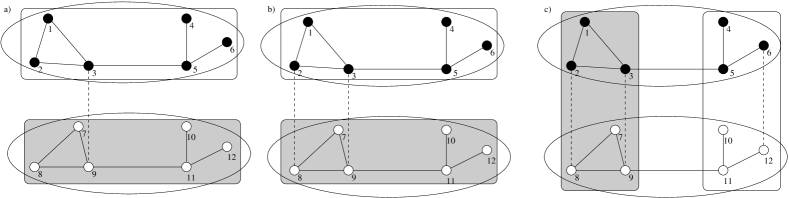
Figure 1: Two graphs with $6$ black and white nodes respectively and $7$ links each are progressively interconnected with a) $1$ interlink, b) $2$ interlinks and c) $3$ interlinks. Adding $1$ or $2$ interlinks causes the Fiedler eigenvector to split (depicted by the rectangles) the network into the natural partitions $G_{1}$ and $G_{2}$ . For both cases, the confining links match the added interlinks (dashed lines). However, when adding $3$ interlinks the Fiedler partition experiences a brusque shift, causing the intralinks of the single networks to become the confining links. Thus the added interlinks become a part of the Fiedler partitions.

III.2 General interlinking

A second important example that may be treated algebraically corresponds to the mean-field approximation of the general interlinking strategy. The mean-field approach consists of studying a graph with two identical networks interacting via $N_{1}^{2}$ weighted connections. The interdependence matrix is a matrix with all unitary components: $B_{12}=J$, where $J$ is the all ones matrix; the weight of each interlink is $\alpha=\frac{L_{12}}{N_{1}^{2}}$, and

$$Q=Q_{A}+\alpha Q_{B}=\left[\begin{array}[]{cc}Q_{1}+\alpha N_{1}I&-\alpha J\\ -\alpha J&Q_{2}+\alpha N_{1}I\end{array}\right].$$ (12)

As in the previous case, the $Q_{B}$ matrix commutes with $Q_{A}$ and hence a common set of eigenvectors can be chosen as in (9). The null eigenvalue $\mu_{N}$ is always present, while all the others experience some increase for a non-trivial $\alpha$: all eigenvalues $\mu_{i}$ for $i$ smaller than $N-1$, increase for a fixed amount $\alpha N_{1}$, while $\mu_{N-1}$ increases by twice that quantity,

$$\left\{\begin{array}[]{ll}\mu_{N}&=0,\\ \mu_{N-1}&=2\alpha N_{1},\\ \mu_{i}&=\omega_{i}+\alpha N_{1}\text{, for $i\leq N-1$. }\end{array}\right.$$ (13)

This different rate of growth again implies that there exists a critical value $\alpha_{J}$ beyond which the second and third eigenvectors ($\mu_{N-1}$ and $\mu_{N-2}$) swap. The threshold $\alpha_{J}$ can be easily calculated imposing the crossing condition $\mu_{N-1}=\mu_{N-2}$:

$$\alpha_{J}=\frac{\omega_{N-1}}{N_{1}}.$$ (14)

With $\alpha=\frac{L_{12}}{N_{1}^{2}}$, the critical number of links for the general interlinking strategy can be also estimated in the mean-field approximation:

$$l_{J}=\alpha_{J}N_{1}^{2}=\omega_{N-1}\cdot N_{1}.$$ (15)

It is worth noting that, the critical number of interlinks corresponding to the mean-field theory of the diagonal (11), and general (15) interlink strategies, differ simply by a factor of $2$.

IV Approximating $\mu_{N-1}$ using perturbation theory

The problem consists in finding the minimum of the associated quadratic form in the unitary sphere ($x^{T}x=1$), with the constraint $u^{T}x=0$.

$$\mu=\mu_{N-1}=\inf_{x\neq 0,u^{T}x=0}\frac{x^{T}Qx}{x^{T}x};$$ (16)

In our case, the matrix $Q$ is the sum of a matrix $Q_{A}$ linking only nodes inside the same net, and a “perturbation” $\alpha Q_{B}$ that only connects nodes in different networks ($Q_{A}+\alpha Q_{B}$). Therefore, we want to find the minimum that satisfies the spectral equations:

$$\left\{\begin{array}[]{rcr}(Q_{A}+\alpha Q_{B}-\mu I)x&=0,\\ x^{T}x&=1,\\ u^{T}x&=0.\end{array}\right.$$ (17)

When the solution is analytical in $\alpha$, one may express $\mu$ and $x$ by Taylor expansion as

$$\mu = \sum_{k=0}^{\infty}\mu^{(k)}\alpha^{k}$$ (18)

$$x = \sum_{k=0}^{\infty}x^{(k)}\alpha^{k}$$ (19)

Substituting the expansion in the eigenvalue equation (16) gives the hierarchy of equations:

$$\left\{\begin{array}[]{lccl}Q_{A}x^{(k)}+\alpha Q_{B}x^{(k-1)}&=&\sum_{i=0}^{k}\mu^{(k-i)}x^{(i)}&\textit{for all k},\\ \sum_{i=0}^{k}x^{(k-i)}x^{(i)}&=&0&\textit{for $k\geq 1$},\\ u^{T}x^{(k)}&=&0&\textit{for all k}.\end{array}\right.$$ (20)

IV.1 Explicit approximations up to the second order

The zero order expansion just provides a simple set of equations:

$$\left\{\begin{array}[]{lll}Q_{A}x^{(0)}&=\mu^{(0)}x^{(0)},\\ x^{(0)}x^{(0)}&=1,\\ u^{T}x^{(0)}&=0.\end{array}\right.$$ (21)

Let $\left(\mu_{N-1}\right)_{A1},\left(\mu_{N-1}\right)_{A2}$ and $\left(x_{N-1}\right)_{A1},\left(x_{N-1}\right)_{A2}$ denote the smallest non-zero eigenvalue and the corresponding eigenvector of $Q_{1},Q_{2}$, respectively. Similarly

$$\left\{\begin{array}[]{lcl}(x_{N_{1}})_{A1}&=&1/\sqrt{N_{1}}(1,1,\ldots,1,0,0,\ldots,0),\\ (x_{N_{2}})_{A2}&=&1/\sqrt{N_{2}}(0,0,\ldots,0,1,1,\ldots,1).\end{array}\right.$$ (22)

will represent the null eigenvectors of network $G_{1}$ and $G_{2}$, respectively. When the networks are put together, any combination of the former is a null eigenvector. Two special combinations are worth employing: the trivial solution corresponding to the constant vector:

$$x_{N}=\frac{1}{\sqrt{N}}(1,\ldots,1)=\sqrt{\frac{N_{1}}{N}}(x_{N_{1}})_{A1}+\sqrt{\frac{N_{2}}{N}}(x_{N_{2}})_{A2}.$$ (23)

and the other combination orthogonal to the former that represents a useful starting point for the perturbation theory:

$$x_{N-1}^{(0)}=x^{(0)}=\frac{1}{\sqrt{N}}(1,\ldots,1,-1,\ldots,-1)=\sqrt{\frac{N_{1}}{N}}(x_{N_{1}})_{A1}-\sqrt{\frac{N_{2}}{N}}(x_{N_{2}})_{A2}.$$ (24)

which satisfies the zero order approximation (21). The zero order approximation to the Fiedler eigenvalue is then null:

$$\mu^{(0)}=0.$$ (25)

The first order approximation equations follow from (20) as:

$$\left\{\begin{array}[]{rcl}Q_{A}x^{(1)}+\alpha Q_{B}x^{(0)}&=&\mu^{(1)}x^{(0)}\\ \left(x^{(0)}\right)^{T}x^{(1)}&=&0\\ u^{T}x^{(1)}&=&0.\end{array}\right.$$ (26)

Taking the projection over $x^{(0)}$ of the first equation of (26), one obtains the first order correction $\mu^{(1)}$ that depends on the zero order eigenvector only:

$$\mu^{(1)}=\left(x^{(0)}\right)^{T}\alpha Q_{B}x^{(0)}$$ (27)

A simple case to analyze is that where only one interlink joins $A_{1}$ with $A_{2}$: $(B_{12})_{ij}=\delta_{ik}\delta_{kj}$; in this case $(d_{1})_{kk}=\delta_{ik}$ and $(d_{2})_{ll}=\delta_{jl}$ and the perturbation estimate gives:

$$\mu^{(1)}=(\frac{1}{2}(1+1)+1)(\eta_{i})^{2}=\frac{2}{N_{1}}\geq\mu_{N-1}(Q).$$ (28)

where $\eta$ is the single net ($N_{1}$ dimensional) unitary vector $\eta\stackrel{{\scriptstyle def}}{{=}}1/\sqrt{N_{1}}(1,1,\ldots,1)$. When $k$ interlinks are included, $Q_{B}$ is just the sum of $k$ contributions of the previous type thus $\mu^{(1)}=\frac{2k}{N_{1}}$. That is, the first order correction to the Fiedler eigenvalue increases linearly with the number of interlinks. The first order correction to the eigenvector can be evaluated from (26) as a solution of the linear equation:

$$Q_{A}x^{(1)}=-\left(\alpha Q_{B}-\mu^{(1)}\right)x^{(0)}.$$ (29)

where the operator $Q_{A}$ is invertible out of its kernel ($Q_{A}v=0$); since $\left(\alpha Q_{B}-\mu^{(1)}\right)x^{(0)}$ is orthogonal to the kernel, (29) is solvable.

The second order equations follow from (20) as

$$\left\{\begin{array}[]{rl}Q_{A}x^{(2)}+\alpha Q_{B}x^{(1)}&=\mu^{(0)}x^{(2)}+\mu^{(1)}x^{(1)}+\mu^{(2)}x^{(0)}\\ \left(x^{(0)}\right)^{T}x^{(2)}+\left(x^{(1)}\right)^{T}x^{(1)}+\left(x^{(2)}\right)^{T}x^{(0)}&=0\\ ux^{(2)}&=0\end{array}\right.$$ (30)

that is, the second order correction is quadratic and equals:

$$\mu^{(2)}=\left(x^{(0)}\right)^{T}\alpha Q_{B}\left(x^{(1)}\right)=-\left(x^{(1)}\right)^{T}Q_{A}\left(x^{(1)}\right)\leq 0.$$ (31)

As expected $\mu^{(2)}$ is negative, thus improving the estimate of the algebraic connectivity. The former perturbation estimates are illustrated in Fig. 2 together with numerical simulations.

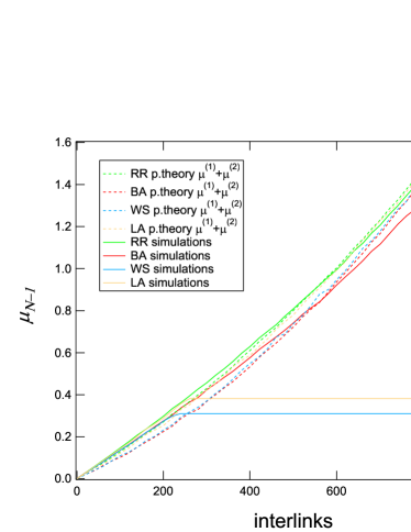
(a) Diagonal strategy

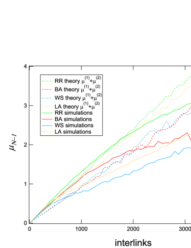
(b) General strategy

Figure 2: Simulated (solid lines) and theorized (dashed lines) algebraic connectivity $\mu_{N-1}$ of four graph models with $N=1000$ nodes, as interlinks are added between single networks following two strategies: diagonal interlinks (left image) and general interlinks (right image). Perturbation theory best approaches $\mu_{N-1}$ for the parabolic region of the diagonal interlinks strategy, which saturates after adding $\frac{\alpha_{Th}\cdot N}{2}$ links, as we detailed in section III.

Perturbation theory may also be applied to any initial eigenvector of the unperturbed networks. Different perturbations $\alpha B$ will have different effects on the quadratic form of (16) associated with all initial eigenvectors. Therefore, it may happen that the perturbed value of $\mu$ obtained starting from $x^{(0)}$ is smaller than the quadratic form associated with the $x_{N-1}$ (the unperturbed eigenvector in (9)) or some other educated guess. This is precisely the origin of the phase transition.

The estimates resulting form the second order perturbation theory are compared in Fig. 2 with the results of numerical calculations. As can be seen, for both the diagonal and the general strategies the agreement is good up to the phase transition where the starting point of the perturbation theory should be changed.

IV.2 Perturbative approximations and upper bounds

Since we are dealing with a constraint optimization problem, finding a minimum of a positive form, any test vector $v$ provides an upper bound for the actual minimum value:

$$\mu=\mu_{N-1}\leq\frac{v^{T}Qv}{v^{T}v}.$$ (32)

The perturbation theory provides natural candidates as test vectors. The zero order solution provides the simplest inequality:

$$\mu_{N-1}(Q)\leq\alpha\frac{(x^{(0)})^{T}Qx^{(0)}}{(x^{(0)})^{T}x^{(0)}}=\alpha\mu^{(1)}.$$ (33)

The first order approximation provides a better (i.e. lower) upper bound:

$$\mu_{N-1}(Q)\leq\frac{(x^{(0)}+\alpha x^{(1)})^{T}Q(x^{(0)}+\alpha x^{(1)})}{(x^{(0)}+\alpha x^{(1)})^{T}(x^{(0)}+\alpha x^{(1)})}.$$

that is:

$$\mu_{N-1}(Q)\leq\frac{\alpha\mu^{(1)}+\alpha^{2}\mu^{(2)}+\alpha^{3}(x^{(1)})^{T}Q_{B}x^{(1)}}{1+\alpha^{2}(x^{(1)})^{2}}.$$ (34)

which for small enough $\alpha$ is always lower than $\alpha\mu^{(1)}$.

V Simulations

Previous sections provided basic means to understand the dependence of the algebraic connectivity on the topology of the interdependence links. In this section we will introduce model networks to test the predictability and the limits of the mean-field and the perturbation approximations.

V.1 Interdependent networks model

Our interdependent network model consists of two main components: a network model for the single networks, and the rules by which the two networks are linked. In other words, to model two interdependent networks one needs to select two model networks and one interlinking strategy.

In the numerical simulations discussed here, we considered four different graph models for our coupled networks. These models exhibit a wide variety of topological features and represent the four different building blocks:

• Random Regular (RR): random configuration model introduced by Bollobas Bollobas2001 . All nodes are initially assigned a fixed degree $d_{i}=k,i\in\mathcal{N}$. The $k$ degree stubs are then randomly interconnected while avoiding self-loops and multiple links.

• Barabási-Albert (BA): growth model proposed by Barabási et. al. A.L.Barabasi1999 whereby new nodes are attached to $m$ already existing nodes in a preferential attachment fashion. For large enough values of $N$, this method ensures the emergence of power-law behavior observed in many real-world networks.

• Watts-Strogatz (WS): randomized circular lattice proposed by Watts et. al. WatStr98 where all nodes start with a fixed degree $k$ and are connected to their $\frac{k}{2}$ immediate neighbors. In a second stage, all existing links are rewired with a small probability $p$, which produces graphs with low average hopcount yet high clustering coefficient, which mimics the small-world property found in real-world networks.

• Lattice (LA): a deterministic three-dimensional grid which loops around its boundaries (i.e. a geometrical torus).

The input parameters for each model are set such that all graphs have the same number of nodes and links. In addition, all simulated graphs consist of a single connected component, i.e. random graphs containing more than one connected component were discarded.

We define two strategies to generate the interdependency matrix $B$, which we analytically solved in section III:

• diagonal interlinking strategy: links are randomly added to the diagonal elements of $B$, thus linking single network’s analogous nodes.

• general interlinking strategy: random links are added to $B$ without restrictions, generating a random interconnection pattern.

In the next sections, we explore the effects of the two interlinking strategies on the Fiedler partition. However, some results can be extended to more complicated situations, including different synthetic networks or more complex linking strategies.

V.2 Partition quality metrics

Let us introduce some preliminary definitions, required for understanding of our numerical results. We define a graph bipartition of $G$ as the two disjoint sets of nodes $\left\{\mathcal{R},\mathcal{S}\right\}$, where $\mathcal{R}\cup\mathcal{S}=\mathcal{N}$. We define the natural partition of $G$ as the partition with the two original node sets: $\mathcal{R}=\mathcal{N}_{1}$, and $\mathcal{S}=\mathcal{N}_{2}$. The number of nodes in $\mathcal{R}$ and $\mathcal{S}$ is counted by their cardinality $\left|\mathcal{R}\right|$ and $\left|\mathcal{S}\right|$, respectively. In addition, we express the number of links with one end node in $\mathcal{R}$ an another end node in $\mathcal{S}$ as $l\left(\mathcal{R},\mathcal{S}\right)=l\left(\mathcal{S},\mathcal{R}\right)$. Fiedler partitioning bisects the nodes in $\mathcal{N}$ into two clusters, such that two nodes $i$ and $j$ belong to the same cluster if ${x_{i}}{x_{j}}>0$, i.e. the corresponding components of the Fiedler eigenvector $x$ have the same sign. For example, if the coupling strength $\alpha$ in (3) is zero, the bipartition resulting from Fiedler partitioning is equivalent to the two natural clusters, i.e. $\mathcal{R}=G_{1}$ and $\mathcal{S}=G_{2}$.

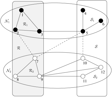
Figure 3: The four main partition sets are displayed: $\mathcal{N}_{1}$ (set of black nodes), $\mathcal{N}_{2}$ (set of white nodes), $\mathcal{R}$ (set of nodes within the gray rectangle), and $\mathcal{S}$ (set of nodes within the white rectangle). Both, the partition sets and the interlinks (dashed lines) were arbitrary chosen for illustration purposes and do not represent the corresponding Fiedler partition.

The intersection between the two single graphs $\left(\mathcal{N}_{1},\mathcal{N}_{2}\right)$ and the Fiedler partitions $\left(\mathcal{R},\mathcal{S}\right)$ of the interdependent network yields four node subsets, defined as follows and illustrated in Fig. 3: (a) $\mathcal{R}_{1}$ as the intersection between the positive Fielder partition and $\mathcal{N}_{1}$, (b) $\mathcal{S}_{1}$ as the intersection between the negative Fielder partition and $\mathcal{N}_{1}$, (c) $\mathcal{R}_{2}$ as the intersection between the positive Fielder partition and $\mathcal{N}_{2}$, (d) $\mathcal{S}_{2}$ as the intersection between the positive Fielder partition and $\mathcal{N}_{2}$. By construction the four defined groups are disjoint, and the union of all groups equals the full set of nodes.

In order to quantify the properties of the Fiedler partition, we study the following set of metrics:

• Fiedler cut-size $\stackrel{{\scriptstyle def}}{{=}}\frac{{l\left({{{\mathcal{R}}},{{\mathcal{S}}}}\right)}}{{{L_{1}}+{L_{2}}}}$. It represents the fraction of links with one end in $\mathcal{R}$ and another end in $\mathcal{S}$ (irrespective of the directionality of the link) over the starting number of links.

• interdependence angle, defined as the angle between the normalized Fielder vector $x$ and the versor $x^{(0)}$, introduced in (23). The interdependence angle is minimized when the Fiedler vector is parallel to the natural partition, i.e. $x^{(0)}$.

• entropy of the squared Fiedler vector components $\mathop{=}\limits^{def}-\sum\nolimits_{i=1}^{N}{{x_{i}}^{2}\log{x_{i}}^{2}}$. Based on Shannon’s information theory metric, the entropy indicates how homogeneous the values in $x$ are, similarly to the participation ratio or vector localization. The higher the entropy, the lower is the dispersion among the values in $x$.

Some partition quality metrics may be undefined if the Laplacian matrix $Q$ is defective Wilkinson1965 . In particular, if the second and third largest eigenvalues of $Q_{A}+\alpha Q_{B}$ are equal $\mu_{N-1}=\mu_{N-2}$ then any linear combination $x^{\prime}=ax_{N-1}+bx_{N-2}$ is also an eigenvector of $Q$ with eigenvalue $\mu_{N-1}$, thus the Fiedler vector is not uniquely defined. However we will ignore these cases, which tend to occur only in graphs with deterministic structures (e.g. the cycle graph VanMieghemSpectra ).

V.3 Diagonal Interlinking Strategy

V.3.1 Strategy Description

The diagonal interlinking strategy consists of adding links between the respective components of two identical networks. We can add as little as $1$ link and as many as $N$ links. This strategy was chosen to achieve the maximum effect by meticulously adding a small number of interlinks. A simplified physical example would be that of two flat metal plates: a hot one, and a cold one. If the objective is to equalize their temperature as fast as possible, we should adjust the plates side by side so as to maximize the heat transfer, which is equivalent to the diagonal interlinks strategy.

V.3.2 Initial and final states

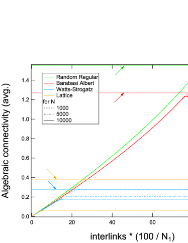
(a) Algebraic Connectivity

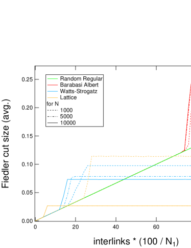
(b) Fiedler cut

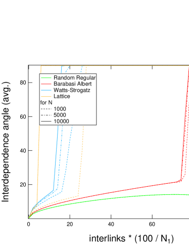
(c) Interdependence angle

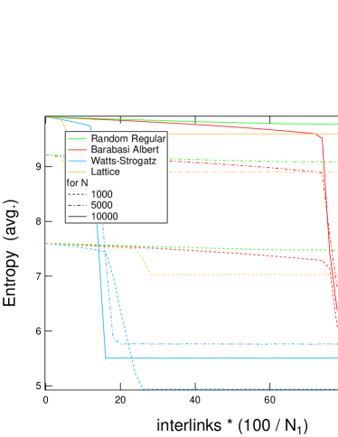
(d) Entropy

Figure 4: (Color online) Four metrics’ averages are displayed to evaluate the effect of adding interlinks following the diagonal strategy: algebraic connectivity ($\mu_{N-1}$), Fiedler cut (${l\left({{{\mathcal{R}}},{{\mathcal{S}}}}\right)}/{{L_{1}}+{L_{2}}}$), interdependence angle ($acos\left(x^{T}x^{(0)}/\left\|x\right\|\left\|x^{(0)}\right\|\right)$), and entropy ($-\sum\nolimits_{i=1}^{N}{{x_{i}}^{2}\log{x_{i}}^{2}}$). All metrics experience a transition that sharpens for increasing $N$. BA and RR graphs transition around $~{}80\%$ added interlinks, whereas WS and LA graphs transition around $~{}20\%$. The size of the network $N_{1}$ has a relatively little impact on BA and RR curves, which suggests that the transition is independent of the network size $N_{1}$. The flat lines signaled with arrows in the top left plot benchmark the average algebraic connectivity of the $N_{1}=1,000$ respective single networks.

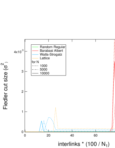
(a) Fiedler cut

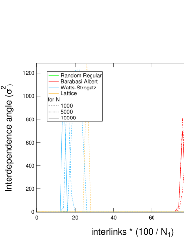
(b) Interdependence angle

Figure 5: (Color online) The fluctuation $\sigma^{2}$ of the Fiedler cut and the interdependence angle are displayed to evaluate the effect of adding interlinks following the diagonal strategy. The narrowing peaks illustrate the sharpening of the transition observed in Fig. 4.

We will refer to the natural, initial or unperturbed state as the scenario where there exist no interlink connecting the two networks $G_{1}$ and $G_{2}$. The left hand side of Fig. 1 and Fig. 4 illustrate the network configuration and partition quality metrics, respectively. In this case the algebraic connectivity dips to a null value, as no communication is possible; the Fiedler partition then becomes undetermined. However, the sign of $x^{(0)}$ in (29) allows splitting the network into two clusters ${\cal P}=G_{1}$ and ${\cal Q}=G_{2}$, corresponding to the isolated component networks.

The final state of the diagonal interlink strategy corresponds to $100\%$ or $N$ added interlinks, thus $B=I$ and the Fiedler vector becomes the vector $\left(x_{N-1}(Q_{1}),x_{N-1}(Q_{1})\right)$, as demonstrated in section III. The final partition depends exclusively on $G_{1}$ and $G_{2}$, independently of $B$. Since we assume $G_{1}=G_{2}$, the final cut consists purely of a subset of intralinks of $A_{1}$, as illustrated in the right hand side of Fig. 1. By adding (or removing) interlinks between the two independent networks we switched from a purely interlink cut to a purely intralink cut, which is the essence of the phase transition.

The sudden partition quality metric shifts reflect the change observed in the Fiedler partition, while providing evidence for the existence of the transition. This is testified by the narrowing of the region where the shifts occurs while increasing (or decreasing) $N$ in Fig. 4. Similarly, the fluctuations of the same quantities exhibit shrinking peaks as can be seen in Fig. 5. Upon increasing the size $N$ of the system, the transition point seems to approach an asymptotic value. As discussed in section III, the mean-field theory predicts this critical value to be $l_{I}=\frac{\mu_{N-1}(Q_{1})\cdot N_{1}}{2}$. Since $\mu_{N-1}(Q_{1})$ has a non-trivial lower bound for increasing $N$ Wu2001 , and its algebraic connectivity is kept unchanged by the perturbation, there will be a critical number of links beyond which $\mu_{N-1}(Q)$ does not change. This critical point corresponds to the transition from an interlink cut to an intralink cut.

The precise location of the jump in the simulated experiment, i.e. the critical value of interlinks per node, depends on the graph model. However, the phase transition is a general phenomenon, which occurrence only depends on the fact that there exists a Fiedler cut for the single networks.

V.3.3 Effect on partition quality metrics

We further investigate the properties of the phase transition by looking at how partition metrics in Fig. 4 evolve as interlinks are added to the $B$ matrix.

The algebraic connectivity starts at its minimum value $\approx\frac{1}{{2N_{1}}}$ as predicted by (28), which grows until it reaches its maximum value $\mu_{N-1}(Q_{1})$ when sufficient interlinks are added. This means that a network with $100\%$ diagonal interlinks and the same network with $90\%$ interlinks synchronize virtually at the same speed. Comparing the final values of the algebraic connectivity, it is remarkable that random networks synchronize faster than lattice networks. This is reasonably due to the longer average distance in the latter.

The Fiedler cut starts at $\frac{1}{{2L_{1}}}$ for a single added interlink. Notice that it increases linearly with the percentage of interlinks, because all added interlinks directly become part of the Fiedler cut. For all networks, we observe a tipping point (which depends on the network type) upon which adding a single link abruptly readjusts the partition: the Fiedler cut switches from pure interlink cutting to a cutting of an invariable set of intralinks. This abrupt change breaks the linearity.

The interdependence angle metric tells us that the Fiedler vector starts being parallel to the first order approximation $x^{(0)}$ for $1$ added interlink. Progressively, the Fiedler vector crawls the $N$-dimensional space up to the transition point, where it abruptly jumps to the final (orthogonal) state $\left(x_{N-1}(Q_{1}),x_{N-1}(Q_{1})\right)$. Similarly to the interdependence angle, the high values of entropy reflect the flatness of $x^{(0)}$, where all components have (almost) the same absolute value. At this initial point, entropy is maximum and almost equal to $log(2N_{1})$, which tells us that the initial partition consists purely of interlinks. When the partition turns to the final state, the entropy is instantly shaped by the network topologies of $A_{1}$ thus dropping to relatively much lower values. Notice that, for all values of $N$, the highest final entropy is attained by the lattice graph due to its regular structure, as seen in Fig. 4.

V.3.4 Network Model Differences

RR and BA synchronize relatively faster than deterministic networks because random interconnections shorten the average hopcount, thus bringing all elements of the network closer (creating the small-world effect WatStr98 ). For the particular case of BA, we observe the emergence of a dominant partition which contains approximately $90\%$ of the total number of nodes.

There exists a significant difference between the $1,000$ node lattice and the $10,000$ node lattice, which is expected due to the variable size response of network models. We conjecture that this difference is caused by the average geodesic distance: the average node distance for a three dimensional lattice lattice graphs grows with $\sqrt[3]{N}$, as opposed to random models, which usually display logarithmic increases. Interestingly, Fig. 4 shows that small lattices synchronize faster than WS, but the situation is soon reversed for higher $N$.

To test whether the phase transition is merely an artifact of our synthetic models, additional simulations were carried out using real topologies from the KONECT dataset. Simulations verify that the transition from the natural partition to the final orthogonal partition also occurs in real networks. However, the transition takes place very early in the link addition process, due to the poor synchronization capabilities of networks not designed for such purpose. The interpretation of such result is that, to provide that real network with a complete backup mirror without synchronization delays, a small number of interlinks are required.

V.4 General Interlinks Strategy

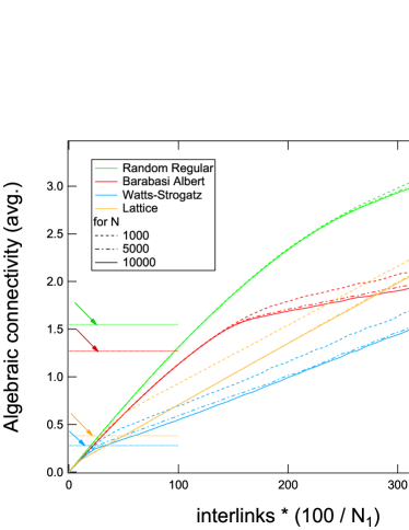
(a) Algebraic Connectivity

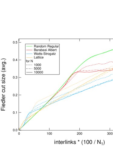
(b) Fiedler cut

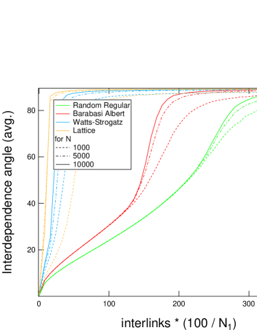
(c) Interdependence angle

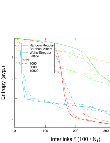
(d) Entropy

Figure 6: (Color online) Four metrics’ averages are displayed to qualitatively evaluate the effect of adding interlinks following the general strategy: algebraic connectivity ($\mu_{N-1}$), Fiedler cut (${l\left({{{\mathcal{R}}},{{\mathcal{S}}}}\right)}/{{L_{1}}+{L_{2}}}$), interdependence angle ($acos\left(x^{T}x^{(0)}/\left\|x\right\|\left\|x^{(0)}\right\|\right)$), and entropy ($-\sum\nolimits_{i=1}^{N}{{x_{i}}^{2}\log{x_{i}}^{2}}$). The four metrics indicate the existence of up to three regimes, but the regime transitions are not as sharp as in the diagonal strategy scenario. The flat lines signaled with arrows in the top left plot represent the average algebraic connectivity of the $N_{1}=1,000$ respective single networks.

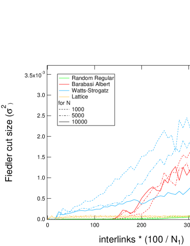
(a) Fiedler cut

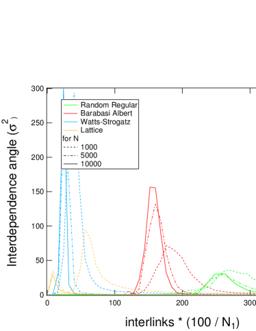
(b) Interdependence angle

Figure 7: (Color online) The fluctuation $\sigma^{2}$ of the Fiedler cut and the interdependence angle are displayed to evaluate the effect of adding interlinks following the general strategy. The increasing Fiedler cut’s fluctuations do not hint the existence of a transition. However the peaking fluctuation displayed by the interdependence angle suggests the presence of a narrowing transition.

V.4.1 Strategy Description

As a variation of the localized diagonal interlinking strategy, our second strategy randomly draws interlinks among any pair of nodes belonging to different networks. Mean-field approximation provides us with exact results, however perturbation analysis loses its power when too many links are added, i.e. the perturbation can no longer be regarded as small. For this reason, we cannot predict an exact asymptotic state as for the diagonal strategy. We have limited our simulations to the inclusion of up to $4$ interlinks per node.

V.4.2 Effect on partition quality metrics

We can observe that the algebraic connectivity of all models experiences two regimes, upon the progressive addition of interlinks as illustrated in Fig. 6. Initially, for a small number of added links, the initial state dips to a minimum as is the case for the diagonal strategy and represents a good starting point for the perturbation theory. As we increase the number of interlinks, the average algebraic connectivity and Fiedler cut curves show a linear increase. At the critical number of links $l_{J}=\mu_{N-1}\cdot N$, the average slope switches regime by damping to half its value, as seen in Fig.6a and Fig. 6b, which is in perfect agreement with our theoretical prediction (12). However not only the average, but also the fluctuations steadily increase, as illustrated by Fig. 7a. High fluctuations are expected, due to the large set of available graph configurations.

As we can see from the interdependence angle in Fig. 6, in the first regime the natural partition is partially preserved up to $l_{J}$. The interdependence angle experiences a sharp increase at the turning point, which further narrows as $N$ increases as seen in Fig. 7b. This is due to the fact that the Fiedler cut in all our isolated model networks scales less than linearly with the network size, which is consistent with the picture of a phase transition between a Fiedler cut dominated by interlinks and an other dominated by intralinks. As opposed to the diagonal strategy, the final eigenvector is not strictly identical to the Fiedler eigenvector of the isolated networks $x_{N-1}$, but it also involves interlink cuts. This is due to the fact that in the general case $x_{N-1}$ does not belong to the kernel of $Q_{B}$ as opposed to the diagonal case.

The exact location of the phase transition can also be predicted employing perturbation theory, by imposing the perturbed value $x_{N-1}(Q)$ of the configuration to be equal to that achieved starting from the $x_{N-1}(Q_{1})$ initial state. However, the resulting formulas are not particularly simple and their numerical calculation requires a time comparable with the Fiedler eigenvalue evaluation of the sparse metrics. For this reasons such estimates are not reported here.

V.4.3 Network Model Differences

Let us focus on the case of adding a small number of interlinks in the range $\left[1,N\right]$. The diagonal strategy will synchronize faster than the general strategy in the case of RR and BA, as illustrated in Fig. 6a. On the other hand, the general strategy synchronizes faster in WS and LA models. Thus if we were to add precisely $N_{1}$ general interlinks between two identical networks, regular structures would (relatively) benefit the most.

For BA, the fraction of intralinks belonging to the Fiedler partition decreases with increasing number of interlinks, whereas the $\frac{\mathcal{R}}{\mathcal{S}}$ ratio increases. This hints that nodes group into high degree clusters (with a high link/node ratio) and a low degree clusters (with a low link/node ratio). In addition, BA’s entropy experiences the highest drop, which indicates that the Fiedler vector is highly localized around a small set of nodes.

The difference between random and grid networks still exists for the general strategy, but it is not as predominant as in the diagonal case. This effect is expected due to the randomization resulting from the random addition of links to regular structures, which is the conceptual basis of the WS model. In general, we observe that the optimal link addition strategy depends on the network topology.

VI Conclusions

This paper aims to provide general results concerning the synchronization of interdependent identical networks. We provided evidence that upon increasing the number of interlinks between two originally isolated networks, their synchronizability experiences a phase transition. That is, there exists a critical number of diagonal interlinks beyond which any further inclusion does not enhance synchronization capabilities at all. Similarly, there exists a critical number of general interlinks beyond which algebraic connectivity increments at half the original rate.

The exact location of the transition depends exclusively on the algebraic connectivity of the graph models, and it is always observed regardless of the interconnected graphs. For the two proposed interconnection strategies, the critical number of interlinks that triggers the transitions can be predicted correctly by mean-field approximations : $\frac{\mu_{N-1}(Q_{1})\cdot N_{1}}{2}$ links for the diagonal interlinks strategy, and $\mu_{N-1}(Q_{1})\cdot N_{1}$ links for the general interlinks strategy. By resorting to perturbation theory we have provided upper bounds for the total algebraic connectivity of the interdependent system and means to estimate it.

This paper beacons a significant starting point to the understanding of the mutual networks synchronization phenomena, as we have just started studying this extremely interesting field. Nonetheless, different linking strategies should be researched and general theory developed. Regarding the mutual synchronization of heterogeneous networks (i.e. $A_{1}\neq A_{2}$), preliminary results confirm the existence of phase transitions with similar features to the general random linkage of identical networks. However, we could not observe any dominant strategy as in the case with the diagonal interlinking.

Acknowledgements

This research has been partly supported by the European project MOTIA (Grant JLS-2009-CIPS-AG-C1-016); the EU Research Framework Programme 7 via the CONGAS project (Grant FP7-ICT 317672); and the EU Network of Excellence EINS (Grant FP7-ICT 288021).

References

- (1) R. A. A. L. Barabasi, Emergence of scaling in random networks, Science 286 (5439) (1999) 509–512.
- (2) D. J. Watts, S. H. Strogatz, Collective dynamics of small world networks, Nature (393) (1998) 440–442.
- (3) C. Huygens, Horologium Oscillatorium, Paris, France, 1673.
- (4) A. Bergen, D. Hill, A structure preserving model for power system stability analysis, Power Apparatus and Systems, IEEE Transactions on PAS-100 (1) (1981) 25 –35.
- (5) P. Van Mieghem, The N-intertwined SIS epidemic network model, Computing 93 (2-4) (2011) 147–169.
- (6) S. Strogatz, From kuramoto to crawford: Exploring the onset of synchronization in populations of coupled oscillators., Physica D 143 (2000) 1–20.
- (7) A. Jadbabaie, N. Motee, M. Barahona, On the Stability of the Kuramoto Model of Coupled Nonlinear Oscillators, in: In Proceedings of the American Control Conference, 2004, pp. 4296–4301.
- (8) J. A. Acebrón, L. L. Bonilla, C. J. Pérez-Vicente, F. Ritort, R. Spigler, The Kuramoto model: A simple paradigm for synchronization phenomena, Rev. Mod. Phys. 77 (2005) 137–185.
- (9) F. M. Atay, T. Biyikoglu, J. Juergen, Synchronization of networks with prescribed degree distributions, IEEE Transactions on Circuits and Systems-I 53 (1) (2006) 92–98.
- (10) J. Chen, J. Lu, C. Zhan, G. Chen, Laplacian Spectra and Synchronization Processes on Complex Networks, Springer Optimization and Its Applications, 2012, Ch. 4, pp. 81–113.
- (11) F. B. Florian Dörfler, Exploring synchronization in complex oscillator networks, Synchronization tutorial paper for 51st IEEE Conference on Decision and Control (CDC).
- (12) X. F. Wang, G. Chen, Synchronization in scale-free dynamical networks: robustness and fragility, Circuits and Systems I: Fundamental Theory and Applications, IEEE Transactions on 49 (1) (2002) 54 –62.
- (13) R. Olfati-Saber, Ultrafast consensus in small-world networks, in: Proceedings of the American Control Conference, IEEE, Los Alamitos, CA, USA, 2005, pp. 2371–2378.
- (14) R. Olfati-Saber, H. Dartmouth Coll., Algebraic connectivity ratio of ramanujan graphs, in: American Control Conference, 2007.
- (15) Simpson-Porco, J. W. Dorfler, B. F. Florian, Droop-controlled inverters are kuramoto oscillators, in: IFAP Workshop on Distributed Estimation and Control of Networked Systems, Vol. 3, 2012, pp. 264–269.
- (16) T. Yamamoto, H. Sato, A. Namatame, Evolutionary optimised consensus and synchronisation networks, IJBIC 3 (3) (2011) 187–197.
- (17) H. Wang, Q. Li, G. D’Agostino, S. Havlin, H. E. Stanley, P. Van Mieghem, Effect of the interconnected network structure on the epidemic threshold, arXiv:1303.0781.
- (18) S. V. Buldyrev, R. Parshani, G. Paul, H. E. Stanley, S. Havlin, Catastrophic cascade of failures in interdependent networks, Nature 464 (7291) (2010) 1025–1028.
- (19) E. A. Leicht, M. D. Raissa, Percolation on interacting networks, arXiv:0907.0894.
- (20) Y. Shang, Synchronization in networks of coupled harmonic oscillators with stochastic perturbation and time delays, Mathematics and its Applications : Annals of the Academy of Romanian Scientists 4 (1) (2012) 44.
- (21) R. Freeman, P. Yang, K. Lynch, Distributed estimation and control of swarm formation statistics, in: American Control Conference, 2006, 2006, pp. 7 pp.–. doi:10.1109/ACC.2006.1655446.
- (22) A. Jamakovic, S. Uhlig, On the relationship between the algebraic connectivity and graph’s robustness to node and link failures, in: Next Generation Internet Networks, 3rd EuroNGI Conference on, Trondheim, Norway, 2007.
- (23) M. Fiedler, A property of eigenvectors of nonnegative symmetric matrices and its application to graph theory, Czechoslovak Mathematical Journal 25.
-
(24)
S. H. Strogatz, Exploring complex
networks, Nature 410 (6825) (2001) 268–276.
doi:10.1038/35065725.
URL http://dx.doi.org/10.1038/35065725 - (25) P. Lin, Y. Jia, Average consensus in networks of multi-agents with both switching topology and coupling time-delay, Physica A: Statistical Mechanics and its Applications 387 (1) (2008) 303 – 313.
- (26) P. Van Mieghem, Graph Spectra for Complex Networks, Cambridge University Press, 2010.
- (27) M. Fiedler, Algebraic connectivity of graphs, Czechoslovak Math 23/98 (1973) 298–305.
- (28) S. J. Blundell, K. M. Blundell, Concepts in thermal physics, Oxford University Press, 2010.
- (29) B. Bollobas, Random Graphs, 2nd Edition, Cambridge University Press, Cambridge, 2001.
- (30) J. Wilkinson, The Algebraic Eigenvalue Problem, Oxford University Press, New York, 1965.
- (31) C. W. Wu, Synchronization in arrays of coupled nonlinear systems: passivity, circle criterion, and observer design, Circuits and Systems I: Fundamental Theory and Applications, IEEE Transactions on 48 (10) (2001) 1257 –1261.