Newton-Based Optimization for Kullback-Leibler Nonnegative Tensor Factorizations

Abstract

Tensor factorizations with nonnegative constraints have found application in analyzing data from cyber traffic, social networks, and other areas. We consider application data best described as being generated by a Poisson process (e.g., count data), which leads to sparse tensors that can be modeled by sparse factor matrices. In this paper we investigate efficient techniques for computing an appropriate canonical polyadic tensor factorization based on the Kullback-Leibler divergence function. We propose novel subproblem solvers within the standard alternating block variable approach. Our new methods exploit structure and reformulate the optimization problem as small independent subproblems. We employ bound-constrained Newton and quasi-Newton methods. We compare our algorithms against other codes, demonstrating superior speed for high accuracy results and the ability to quickly find sparse solutions.

1 Introduction

Multilinear models have proved useful in analyzing data in a variety of fields. We focus on data that derives from a Poisson process, such as the number of packets sent from one IP address to another on a specific port [36], the number of papers published by an author at a given conference [15], or the count of emails between users in a given time period [3]. Data in these applications is nonnegative and often quite sparse, i.e., most tensor elements have a count of zero. The tensor factorization model corresponding to such sparse count data is computed from a nonlinear optimization problem that minimizes the Kullback-Leibler (K-L) divergence function and contains nonnegativity constraints on all variables.

In this paper we show how to make second-order optimization methods suitable for Poisson-based tensor models of large sparse count data. Multiplicative update is one of the most widely implemented methods for this model, but it suffers from slow convergence and inaccuracy in discovering the underlying sparsity. In large sparse tensors, the application of nonlinear optimization techniques requires consideration of sparsity and problem structure to get better performance. We show that, by exploiting the partial separability of the subproblems, we can successfully apply second-order methods. We develop algorithms that scale to large sparse tensor applications and are quick in identifying sparsity in the factors of the model.

There is a need for second-order methods because computing factor matrices to high accuracy, as measured by satisfaction of the first-order KKT conditions, is effective in revealing sparsity. By contrast, multiplicative update methods can make elements small but are slow to reach the variable bound at zero, forcing the user to guess when “small” means zero. We demonstrate that guessing a threshold is inherently difficult, making the high accuracy obtained with second-order methods desirable.

We start from a standard Gauss-Seidel alternating block framework and show that each block subproblem is further separable into a set of independent functions, each of which depends on only a subset of variables. We optimize each subset of variables independently, an obvious idea which has nevertheless not previously appeared in the setting of sparse tensors. We call this a row subproblem formulation because the subset of variables corresponds to one row of a factor matrix. Each row subproblem amounts to minimizing a strictly convex function with nonnegativity constraints, which we solve using two-metric gradient projection techniques and exact or approximate second-order information.

The importance of the row subproblem formulation is demonstrated in Section 4.1, where we show that applying a second-order method directly to the block subproblem is highly inefficient. We provide evidence that a more effective way to apply second-order methods is through the use of the row subproblem formulation.

Our contributions in this paper are as follows:

1. A new formulation for nonnegative tensor factorization based on the Kullback-Leibler divergence objective that allows for the effective use of second-order optimization methods. The optimization problem is separated into row subproblems containing $R$ variables, where $R$ is the number of factors in the model. The formulation makes row subproblems independent, suggesting a parallel method, although we do not explore parallelism in this paper.

2. Two Matlab algorithms for computing factorizations of sparse nonnegative tensors: one using second derivatives and the other using limited-memory quasi-Newton approximations. The algorithms are made robust with an Armijo line search, damping modifications when the Hessian is ill conditioned, and projections to the bound of zero based on two-metric gradient projection ideas in [6]. The two algorithms have different computational costs: the second derivative method is preferred when $R$ is small, and the quasi-Newton when $R$ is large.

3. Test results that compare the performance of our two new algorithms with the best available multiplicative update method and a related quasi-Newton algorithm that does not formulate using row subproblems. The most significant test results are reported in this paper; detailed results of all experiments are available in the supplementary material (Appendix B).

4. Test results showing the ability of our methods to quickly and accurately determine which elements of the factorization model are zero without using problem-specific thresholds.

The paper is outlined as follows: the remainder of Section 1 surveys related work and provides a review of basic tensor properties. Section 2 formalizes the Poisson nonnegative tensor factorization optimization problem, shows how the Gauss-Seidel alternating block framework can be applied, and converts the block subproblem into independent row subproblems. Section 3 outlines two algorithms for solving the row subproblem, one based on the damped Hessian (PDN-R for projected damped Newton), and one based on a limited-memory approximation (PQN-R for projected quasi-Newton). Section 4 details numerical results on synthetic and real data sets and quantifies the accuracy of finding a truly sparse factorization. Additional test results are available in the supplementary material. Section 5 contains a summary of the paper and concluding remarks.

1.1 Related Work

In this paper, we specifically consider nonnegative tensor factorization (NTF) in the case of the canonical polyadic (also known as CANDECOMP/PARAFAC) tensor decomposition. Our focus is on the K-L divergence objective function, but we also mention related work for the least squares (LS) case. Additionally, we consider related work for nonnegative matrix factorization (NMF) for both K-L and LS. Note that there is much more work in the LS case, but the K-L objective function is different enough that it deserves its own attention. We do not discuss other decompositions such as Tucker.

NMF in the LS case was first proposed by Paatero and Tapper [32] and also studied by Bro [7, p. 169]. Lee and Seung later consider the problem for both LS and K-L formulations and introduce multiplicative updates based on the convex subproblems [25, 26]. Their work is extended to tensors by Welling and Weber [39]. Many other works have been published on the LS versions of NMF [27, 21, 22, 32, 44] and NTF [8, 12, 16, 23, 40].

Lee and Seung’s multiplicative update method [25, 26, 39] is the basis for most NTF algorithms that minimize the K-L divergence function. Chi and Kolda provide an improved multiplicative update scheme for K-L that addresses performance and convergence issues as elements approach zero [11]; we compare to their method in Section 4. By interpreting the K-L divergence as an alternative Csiszar-Tusnady procedure, Zafeiriou and Petrou [41] provide a probabilistic interpretation of NTF along with a new multiplicative update scheme. The multiplicative update is equivalent to a scaled steepest-descent step [26], so it is a first-order optimization method. Since our method uses second-order information, it allows for convergence to higher accuracy and a better determination of sparsity in the factorization.

Second-order information has been used before in connection with the K-L objective. Zdunek and Cichocki [42, 43] propose a hybrid method for blind source separation applications via NMF that uses a damped Hessian method similar to ours. They recognize that the Hessian of the K-L objective has a block diagonal structure but do not reformulate the optimization problem further as we do. Consequently, their Hessian matrix is large, and they switch to the LS objective function for the larger mode of the matrix because their Newton method cannot scale up. Mixing objective functions in this manner is undesirable because it combines two different underlying models. As a point of comparison, a problem in [43] of size $200\times 1000$ is considered too large for their Newton method, but our algorithms can factor a data set of this size with $R=50$ components to high accuracy in less than ten minutes (see the supplementary material). The Hessian-based method in [43] has most of the advanced optimization features that we use (though details differ), including an Armijo line search, active set identification, and an adjustable Hessian damping factor. We also note that Zheng and Zhang [44] compute a damped Hessian search direction and find an iterate with a backtracking line search, though this work is for the LS objective in NMF.

Recently, Hsiel and Dhillon [19] reported algorithms for NMF with both LS and K-L objectives. Their method updates one variable at a time, solving a nonlinear scalar function using Newton’s method with a constant step size. They achieve good performance for the LS objective by taking the variables in a particular order based on gradient information; however, for the more complex K-L objective, they must cycle through all the variables one by one. Our algorithms solve convex row subproblems with $R$ variables using second-order information; solving these subproblems one variable at a time by coordinate descent will likely have a much slower rate of convergence [30, pp. 230-231].

A row subproblem reformulation similar to ours is noted in earlier papers exploring the LS objective, but it never led to Hessian-based methods that exploit sparsity as ours do. Gonzales and Zhang use the reformulation with a multiplicative update method for NMF [17] but do not generalize to tensors or the K-L objective. Phan et al. [33] note the reformulation is suitable for parallelizing a Hessian-based method for NTF using LS. Kim and Park use the reformulation for NTF with LS [23], deriving small bound-constrained LS subproblems. Their method solves the LS subproblems by exact matrix factorization, without exploiting sparsity, and features a block principal pivoting method for choosing the active set. Other works solve the LS objective by taking advantage of row-by-row or column-by-column subproblem decomposition [12, 28, 34].

Our algorithms are similar in spirit to the work of Kim, Sra and Dhillon [20], which applies a projected quasi-Newton algorithm (called PQN in this paper) to solving NMF with a K-L objective. Like PQN, our algorithms identify active variables, compute a Newton-like direction in the space of free variables, and find a new iterate using a projected backtracking line search. We differ from PQN in reformulating the subproblem and in computing a damped Newton direction; both improvements make a huge difference in performance for large-scale tensor problems. We compare to PQN in Section 4.

All-at-once optimization methods, including Hessian-based algorithms, have been applied to NTF with the LS objective function. As an example, Paatero replaces the nonnegativity constraints with a barrier function [31] to yield an unconstrained optimization problem, and Phan, Tichavsky and Cichocki [34] apply a fast damped Gauss-Newton algorithm for minimizing a similar penalized objective. We are not aware of any work on all-at-once methods for the K-L objective in NTF.

Finally, we note that all methods, including ours, find only a locally optimal solution to the NTF problem. Finding the global solution is generally much harder; for instance, Vavasis [38] proves it is NP-hard for an NMF model that fits the data exactly.

1.2 Tensor Review

For a thorough introduction to tensors, see [24] and references therein; we only review concepts that are necessary for understanding this paper. A tensor is a multidimensional array. An $N$-way tensor $\bm{\mathscr{{X}}}$ has size $I_{1}\times I_{2}\times\ldots\times I_{N}$. To differentiate between tensors, matrices, vectors, and scalars, we use the following notational convention: $\bm{\mathscr{{X}}}$ is a tensor (bold, capitalized, calligraphic), ${\bm{\mathbf{{X}}}}$ is a matrix (bold, capitalized), ${\bm{\mathbf{{x}}}}$ is a vector (bold, lowercase), and $x$ is a scalar (lowercase). Additionally, given a matrix ${\bm{\mathbf{{X}}}}$, ${\bm{\mathbf{{x}}}}_{j}$ denotes its $j$th column and $\hat{{\bm{\mathbf{{x}}}}}_{i}$ denotes its $i$th row.

Just as a matrix can be decomposed into a sum of outer products between two vectors, an $N$-way tensor can be decomposed into a sum of outer products between $N$ vectors. Each of these outer products (called components) yields an $N$-way tensor of rank one. The CP (CANDECOMP/PARAFAC) decomposition [10, 18] represents a tensor as a sum of rank-one tensors (see Figure 1):

$$\bm{\mathscr{{X}}}\approx\left\llbracket{\bm{\mathbf{{\lambda}}}};{\bm{\mathbf{{A}}}}^{(1)},\dots,{\bm{\mathbf{{A}}}}^{(N)}\right\rrbracket=\sum_{r=1}^{R}\lambda_{r}\,{\bm{\mathbf{{a}}}}^{(1)}_{r}\circ\ldots\circ{\bm{\mathbf{{a}}}}^{(N)}_{r}$$ (1)

where ${\bm{\mathbf{{\lambda}}}}$ is a vector and each ${\bm{\mathbf{{A}}}}^{(n)}$ is an $I_{n}\times R$ factor matrix containing the $R$ vectors contributed to the outer products by mode $n$, i.e.,

$${\bm{\mathbf{{A}}}}^{(n)}=[{\bm{\mathbf{{a}}}}^{(n)}_{1}\cdots{\bm{\mathbf{{a}}}}^{(n)}_{R}].$$ (2)

Equality holds in (1) when $R$ equals the rank of $\bm{\mathscr{{X}}}$, but often a tensor is approximated by a smaller number of terms. We let ${\bm{\mathbf{{i}}}}$ denote the multi-index $(i_{1},i_{2},\ldots,i_{N})$ of an element ${x}_{\mathbf{i}}$ of $\bm{\mathscr{{X}}}$.

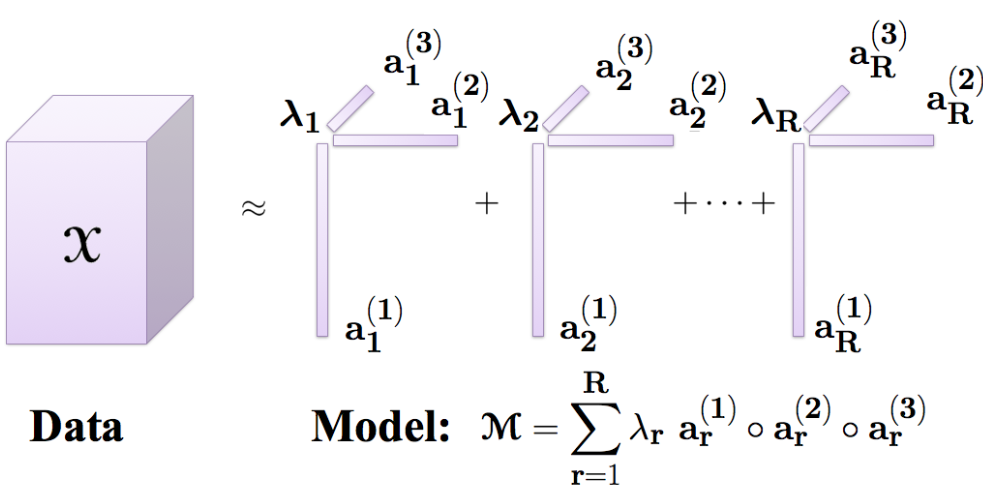
Fig. 1: CANDECOMP/PARAFAC decomposition of a three-way tensor into $R$ components.

We use of the idea of matricization, or unfolding a tensor into a matrix. Specifically, unfolding along mode $n$ yields a matrix of size $I_{n}\cdot J_{n}$, where

$$J_{n}=I_{1}\cdot I_{2}\;\cdots\;I_{n-1}\cdot I_{n+1}\;\cdots\;I_{N-1}\cdot I_{N}.$$

We use the notation ${\bm{\mathbf{{X}}}}_{(n)}$ to represent a tensor $\bm{\mathscr{{X}}}$ that has been unfolded so that its $n$th mode forms the rows of the matrix, and $x^{(n)}_{ij}$ for its $(i,j)$ element. If a tensor $\bm{\mathscr{{X}}}$ is written in Kruskal form (1), then the mode-$n$ matricization is given by

$${\bm{\mathbf{{X}}}}_{(n)}={\bm{\mathbf{{A}}}}^{(n)}{\bm{\mathbf{{\Lambda}}}}({\bm{\mathbf{{A}}}}^{(N)}\odot\ldots\odot{\bm{\mathbf{{A}}}}^{(n+1)}\odot{\bm{\mathbf{{A}}}}^{(n-1)}\odot\ldots\odot{\bm{\mathbf{{A}}}}^{(1)})^{T}$$ (3)

where ${\bm{\mathbf{{\Lambda}}}}=\text{diag}({\bm{\mathbf{{\lambda}}}})$ and $\odot$ denotes the Khatri-Rao product [24].

Tensor results are generally easier to interpret when the factors (2) are sparse. Moreover, many sparse count applications can reasonably expect sparsity in the factors. For example, the 3-way data considered in [15] counts publications by authors at various conferences over a ten year period. The tensor representation has a sparsity of 0.14% (only 0.14% of the data elements are nonzero), and the factors computed by our algorithm with $R=60$ (see Section 4.2) have sparsity 9.3%, 2.7%, and 77.5% over the three modes. One meaning of sparsity in the factors is to say that a typical outer product term connects about 9% of the authors with 3% of the conferences in 8 of the 10 years. Linking particular authors and conferences is an important outcome of the tensor analysis, requiring clear distinction between zero and nonzero elements in the factors.

2 Poisson Nonnegative Tensor Factorization

In this section we state the optimization problem, examine its structure, and show how to separate it into simpler subproblems.

2.1 Gauss-Seidel Alternating Block Formulation

We seek a tensor model in CP form to approximate data $\bm{\mathscr{{X}}}$:

$$\bm{\mathscr{{X}}}\approx\bm{\mathscr{{M}}}=\left\llbracket{\bm{\mathbf{{\lambda}}}};{\bm{\mathbf{{A}}}}^{(1)},\dots,{\bm{\mathbf{{A}}}}^{(N)}\right\rrbracket=\sum_{r=1}^{R}\lambda_{r}\,{\bm{\mathbf{{a}}}}^{(1)}_{r}\circ\ldots\circ{\bm{\mathbf{{a}}}}^{(N)}_{r}.$$

The value of $R$ is chosen empirically, and the scaling vector ${\bm{\mathbf{{\lambda}}}}$ and factor matrices ${\bm{\mathbf{{A}}}}^{(n)}$ are the model parameters that we compute.

In [11], it is shown that a K-L divergence objective function results when data elements follow Poisson distributions with multilinear parameters. The best-fitting tensor model under this assumption satisfies:

$$\min_{{\bm{\mathbf{{\lambda}}}},{\bm{\mathbf{{A}}}}^{(1)},\ldots,{\bm{\mathbf{{A}}}}^{(N)}}\; f(\bm{\mathscr{{M}}})=\sum_{{\bm{\mathbf{{i}}}}}{m}_{\mathbf{i}}-{x}_{\mathbf{i}}\log{m}_{\mathbf{i}}$$

s.t. $$\displaystyle\bm{\mathscr{{M}}}=\sum_{r=1}^{R}\lambda_{r}\,{\bm{\mathbf{{a}}}}^{(1)}_{r}\circ\ldots\circ{\bm{\mathbf{{a}}}}^{(N)}_{r},$$ (4)

$$\lambda_{r}\geq 0,{\bm{\mathbf{{a}}}}^{(n)}_{r}\geq 0,\|{\bm{\mathbf{{a}}}}^{(n)}_{r}\|_{1}=1,\;\;\forall r\in\{1,\ldots R\},\;\forall n\in\{1,\ldots N\},$$

where ${x}_{\mathbf{i}}$ denotes element $(i_{1},\ldots,i_{n})$ of tensor $\bm{\mathscr{{X}}}$ and ${m}_{\mathbf{i}}$ denotes element $(i_{1},\ldots,i_{n})$ of the model $\bm{\mathscr{{M}}}$. The model may have terms where ${m}_{\mathbf{i}}=0$ and ${x}_{\mathbf{i}}=0$; for this case we define $0\log 0=0$. Note that for matrix factorization, (4) reduces to the K-L divergence used by Lee and Seung [25, 26]. The constraint that normalizes the column sum of the factor matrices serves to remove an inherent scaling ambiguity in the CP factor model.

As in [11], we unfold $\bm{\mathscr{{X}}}$ and $\bm{\mathscr{{M}}}$ into their $n$th matricized mode, and use (3) to express the objective as

$$f(\bm{\mathscr{{M}}})={\bm{\mathbf{{e}}}}^{T}[{\bm{\mathbf{{A}}}}^{(n)}{\bm{\mathbf{{\Lambda}}}}{\bm{\mathbf{{\Pi}}}}^{(n)}-{\bm{\mathbf{{X}}}}_{(n)}\ast\log({\bm{\mathbf{{A}}}}^{(n)}{\bm{\mathbf{{\Lambda}}}}{\bm{\mathbf{{\Pi}}}}^{(n)})]{\bm{\mathbf{{e}}}}\;,$$

where ${\bm{\mathbf{{e}}}}$ is a vector of all ones, the operator $\ast$ denotes elementwise multiplication, $\log(\cdot)$ is taken elementwise,

$${\bm{\mathbf{{\Pi}}}}^{(n)} = ({\bm{\mathbf{{A}}}}^{(N)}\odot\ldots\odot{\bm{\mathbf{{A}}}}^{(n+1)}\odot{\bm{\mathbf{{A}}}}^{(n-1)}\odot\ldots\odot{\bm{\mathbf{{A}}}}^{(1)})^{T}\in{\bf R}^{R\times J_{n}}\;,\;\mbox{and}$$ (5)

$${\bm{\mathbf{{\Lambda}}}} = \text{diag}({\bm{\mathbf{{\lambda}}}})\in{\bf R}^{R\times R}.$$

Note that by expanding the Khatri-Rao products in (5) and remembering that column vectors ${\bm{\mathbf{{a}}}}^{(n)}_{r}$ are normalized, each row of ${\bm{\mathbf{{\Pi}}}}^{(n)}$ conveniently sums to one. This is a consequence of using the $\ell_{1}$ norm in (4).

The above representation of the objective motivates the use of an alternating block optimization method where only one factor matrix is optimized at a time. Holding the other factor matrices fixed, the optimization problem for ${\bm{\mathbf{{A}}}}^{(n)}$ and ${\bm{\mathbf{{\Lambda}}}}$ is

$$\begin{split}\min_{{\bm{\mathbf{{\Lambda}}}},{\bm{\mathbf{{A}}}}^{(n)}}\;&f({\bm{\mathbf{{\Lambda}}}},\;{\bm{\mathbf{{A}}}}^{(n)})={\bm{\mathbf{{e}}}}^{T}[{\bm{\mathbf{{A}}}}^{(n)}{\bm{\mathbf{{\Lambda}}}}{\bm{\mathbf{{\Pi}}}}^{(n)}-{\bm{\mathbf{{X}}}}_{(n)}\ast\log({\bm{\mathbf{{A}}}}^{(n)}{\bm{\mathbf{{\Lambda}}}}{\bm{\mathbf{{\Pi}}}}^{(n)})]{\bm{\mathbf{{e}}}}\\ \text{s.t.}\quad&{\bm{\mathbf{{\Lambda}}}}\geq 0,\;{\bm{\mathbf{{A}}}}^{(n)}\geq 0,\;{\bm{\mathbf{{e}}}}^{T}{\bm{\mathbf{{A}}}}^{(n)}={\bm{\mathbf{{1}}}}.\end{split}$$ (6)

Problem (6) is not convex. However, ignoring the equality constraint and letting ${\bm{\mathbf{{B}}}}^{(n)}={\bm{\mathbf{{A}}}}^{(n)}{\bm{\mathbf{{\Lambda}}}}$, we have

$$\min_{{\bm{\mathbf{{B}}}}^{(n)}\geq 0}\;\;f({\bm{\mathbf{{B}}}}^{(n)})={\bm{\mathbf{{e}}}}^{T}[{\bm{\mathbf{{B}}}}^{(n)}{\bm{\mathbf{{\Pi}}}}^{(n)}-{\bm{\mathbf{{X}}}}_{(n)}\ast\log({\bm{\mathbf{{B}}}}^{(n)}{\bm{\mathbf{{\Pi}}}}^{(n)})]{\bm{\mathbf{{e}}}}$$ (7)

which is convex with respect to ${\bm{\mathbf{{B}}}}^{(n)}$. The two formulations are equivalent in that a KKT point of (7) can be used to find a KKT point of (6). Chi and Kolda show in [11] that (7) is strictly convex given certain assumptions on the sparsity pattern of ${\bm{\mathbf{{X}}}}_{(n)}$.

We pause to think about (7) when the tensor is two-way. In this case, we solve for two factor matrices by alternating over two block subproblems; for instance, with $n=1$ the subproblem (7) finds ${\bm{\mathbf{{B}}}}^{(1)}$ with ${\bm{\mathbf{{\Pi}}}}^{(1)}=({\bm{\mathbf{{A}}}}^{(2)})^{T}$. For an $N$-way problem, the only change to (7) is ${\bm{\mathbf{{\Pi}}}}^{(n)}$, which grows in size exponentially with each additional factor matrix. To efficiently solve the subproblems (7) for large sparse tensors we can exploit sparsity to reduce the computational costs. As discussed in the next section, columns of ${\bm{\mathbf{{\Pi}}}}^{(n)}$ need to be computed only when the corresponding column in the unfolded tensor ${\bm{\mathbf{{X}}}}_{(n)}$ has a nonzero element. Our row subproblem formulation carries this idea further because each row subproblem generally uses only a fraction of the nonzero elements in ${\bm{\mathbf{{X}}}}_{(n)}$.

At this point we define Algorithm 1, a Gauss-Seidel alternating block method. The algorithm iterates over each mode of the tensor, solving the convex optimization block subproblem. Steps 6 and 7 rescale the factor matrix columns, redistributing the weight into ${\bm{\mathbf{{\lambda}}}}$. For the moment, we leave the subproblem solution method in Step 5 unspecified. A proof that Algorithm 1 convergences to a local minimum of (4) is given in [11].

Algorithm 1 Alternating Block Framework

Given data tensor $\bm{\mathscr{{X}}}$ of size $I_{1}\times I_{2}\times\cdots\times I_{N}$, and the number of components $R$
Return a model $\bm{\mathscr{{M}}}=[{\bm{\mathbf{{\lambda}}}};{\bm{\mathbf{{A}}}}^{(1)}\ldots{\bm{\mathbf{{A}}}}^{(N)}]$

1:Initialize ${\bm{\mathbf{{A}}}}^{(n)}\in{\bf R}^{I_{n}\times R}$ for $n=1,\ldots,N$

2:repeat

3:     for $n=1,\dots,N$ do

4:         Let ${\bm{\mathbf{{\Pi}}}}^{(n)}=({\bm{\mathbf{{A}}}}^{(N)}\odot\ldots\odot{\bm{\mathbf{{A}}}}^{(n+1)}\odot{\bm{\mathbf{{A}}}}^{(n-1)}\odot\ldots\odot{\bm{\mathbf{{A}}}}^{(1)})^{T}$

5:         Use Algorithm 2 to compute ${\bm{\mathbf{{B}}}}^{*}$ that minimizes $f({\bm{\mathbf{{B}}}}^{(n)})$ s.t. ${\bm{\mathbf{{B}}}}^{(n)}\geq 0$

6:         ${\bm{\mathbf{{\lambda}}}}\leftarrow\textbf{e}^{T}{\bm{\mathbf{{B}}}}^{*}$

7:         ${\bm{\mathbf{{A}}}}^{(n)}\leftarrow{\bm{\mathbf{{B}}}}^{*}{\bm{\mathbf{{\Lambda}}}}^{-1},\;$ where ${\bm{\mathbf{{\Lambda}}}}=\text{diag}({\bm{\mathbf{{\lambda}}}})$

8:     end for

9:until all mode subproblems have converged

This outline of Algorithm 1 corresponds exactly with the method proposed in [11]; where we differ is in how to solve subproblem (7) in Step 5. Note also that this algorithm is the same as for the least squares objective (references were given in Section 1.1); there the subproblem in Step 5 is replaced by a linear least squares subproblem. We now proceed to describe our method for solving (7).

2.2 Row Subproblem Reformulation

We examine the objective function $f({\bm{\mathbf{{B}}}}^{(n)})$ in (7) and show that it can be reformulated into independent functions. As mentioned in the previous section, rows of ${\bm{\mathbf{{\Pi}}}}^{(n)}$ sum to one if the columns of factor matrices are nonnegative and sum to one. When ${\bm{\mathbf{{\Pi}}}}^{(n)}$ is formed at Step 4 of Algorithm 1, the factor matrices satisfy these conditions by virtue of Steps 6 and 7; hence, the first term of $f({\bm{\mathbf{{B}}}}^{(n)})$ is

$${\bm{\mathbf{{e}}}}^{T}{\bm{\mathbf{{B}}}}^{(n)}{\bm{\mathbf{{\Pi}}}}^{(n)}{\bm{\mathbf{{e}}}}\;=\;{\bm{\mathbf{{e}}}}^{T}{\bm{\mathbf{{B}}}}^{(n)}{\bm{\mathbf{{e}}}}\;=\;\sum_{i=1}^{I_{n}}\sum_{r=1}^{R}b^{(n)}_{ir}.$$

The second term of $f({\bm{\mathbf{{B}}}}^{(n)})$ is a sum of elements from the $I_{n}\times J_{n}$ matrix ${\bm{\mathbf{{X}}}}_{(n)}\ast\log({\bm{\mathbf{{B}}}}^{(n)}{\bm{\mathbf{{\Pi}}}}^{(n)})$. Recall that the operations in this expression are elementwise, so the scalar matrix element $(i,j)$ of the term can be written as

$$x^{(n)}_{ij}\log\left(\sum_{r=1}^{R}b^{(n)}_{ir}\pi^{(n)}_{rj}\right).$$

Adding all the elements and combining with the first term gives

$$f({\bm{\mathbf{{B}}}}^{(n)}) = \sum_{i=1}^{I_{n}}\sum_{r=1}^{R}b^{(n)}_{ir}-\sum_{i=1}^{I_{n}}\sum_{j=1}^{J_{n}}x^{(n)}_{ij}\log\left(\sum_{r=1}^{R}b^{(n)}_{ir}\pi^{(n)}_{rj}\right)$$

$$= \sum_{i=1}^{I_{n}}f_{\rm row}({\bm{\hat{\mathbf{{b}}}}}_{i}^{(n)},{\bm{\hat{\mathbf{{x}}}}}_{i}^{(n)},{\bm{\mathbf{{\Pi}}}}^{(n)}).$$

where ${\bm{\hat{\mathbf{{b}}}}}_{i}$ and ${\bm{\hat{\mathbf{{x}}}}}_{i}$ are the $i$th row vectors of their corresponding matrices, and

$$f_{\rm row}({\bm{\hat{\mathbf{{b}}}}},{\bm{\hat{\mathbf{{x}}}}},{\bm{\mathbf{{\Pi}}}})=\sum_{r=1}^{R}\hat{b}_{r}-\sum_{j=1}^{J_{n}}\hat{x}_{j}\log\left(\sum_{r=1}^{R}\hat{b}_{r}\pi_{rj}\right).$$ (8)

Problem (7) can now be rewritten as

$$\min_{{\bm{\hat{\mathbf{{b}}}}}_{1},\ldots,{\bm{\hat{\mathbf{{b}}}}}_{I_{n}}\;\geq 0}\;\;\sum_{i=1}^{I_{n}}f_{\rm row}({\bm{\hat{\mathbf{{b}}}}}_{i}^{(n)},{\bm{\hat{\mathbf{{x}}}}}_{i}^{(n)},{\bm{\mathbf{{\Pi}}}}^{(n)}).$$ (9)

This is a completely separable set of $I_{n}$ row subproblems, each one a convex nonlinear optimization problem containing $R$ variables. The relatively small number of variables makes second-order optimization methods tractable, and that is the direction we pursue in this paper. Algorithm 2 describes how the reformulation fits into Algorithm 1.

Algorithm 2 Row Subproblem Framework for Solving (9)

Given ${\bm{\mathbf{{X}}}}_{(n)}$ of size $I_{n}\times J_{n}$, and ${\bm{\mathbf{{\Pi}}}}^{(n)}$ of size $R\times J_{n}$
Return a solution ${\bm{\mathbf{{B}}}}^{*}$ consisting of row vectors ${\bm{\hat{\mathbf{{b}}}}}_{1}^{*},\ldots,{\bm{\hat{\mathbf{{b}}}}}_{I_{N}}^{*}$

1:for $i=1,\dots,I_{n}$ do

2:     Select row ${\bm{\hat{\mathbf{{x}}}}}_{i}$ of ${\bm{\mathbf{{X}}}}_{(n)}$

3:     Generate one column of ${\bm{\mathbf{{\Pi}}}}^{(n)}$ for each nonzero in ${\bm{\hat{\mathbf{{x}}}}}_{i}$

4:     Use Algorithm 3 or 4 to compute ${\bm{\hat{\mathbf{{b}}}}}_{i}^{*}$ that solves

$$\min\;f_{\rm row}({\bm{\hat{\mathbf{{b}}}}}_{i}^{(n)},{\bm{\hat{\mathbf{{x}}}}}_{i}^{(n)},{\bm{\mathbf{{\Pi}}}}^{(n)})\;\;\mbox{subject to}\;\;{\bm{\hat{\mathbf{{b}}}}}_{i}\geq 0$$

5:end for

The independence of row subproblems is crucial for handling large tensors. For example, if a three-way tensor of size $1000\times 1000\times 1000$ is factored into $R=100$ components, then ${\bm{\mathbf{{\Pi}}}}^{(n)}$ is a $100\times 10^{6}$ matrix. However, elements of ${\bm{\mathbf{{\Pi}}}}^{(n)}$ appear in the optimization objective only where the matricized tensor ${\bm{\mathbf{{X}}}}_{(n)}$ has nonzero elements, so in a sparse tensor many columns of ${\bm{\mathbf{{\Pi}}}}^{(n)}$ can be ignored; this point was first published in [11]. Algorithm 2 exploits this fact in Step 3.

Algorithm 2 also points the way to a parallel implementation of the CP tensor factorization. We note, as did [33], that each row subproblem can be run in parallel and storage costs are determined by the sparsity of the data. In a distributed computing architecture, an algorithm could identify the nonzero elements of each row subproblem at the beginning of execution and collect only the data needed to form appropriate columns of ${\bm{\mathbf{{\Pi}}}}^{(n)}$ at a given processing element. We do not implement a parallel version of the algorithm in this paper.

3 Solving the Row Subproblem

In this section we show how to solve the row subproblem (9) using second-order information. We describe two algorithms, one applying second derivatives in the form of a damped Hessian matrix, and the other using a quasi-Newton approximation of the Hessian. Both algorithms use projection, but the details differ.

Each row subproblem consists of minimizing a strictly convex function of $R$ variables with nonnegativity constraints. One of the most effective methods for solving bound-constrained problems is second-order gradient projection; see [35]. We employ a form of two-metric gradient projection from Bertsekas [6]. Each variable is marked in one of three states based on its gradient and current location: fixed at its bound of zero, allowed to move in the direction of steepest-descent, or free to move along a Newton or quasi-Newton search direction. Details are in Section 3.1.

An alternative to Bertsekas is to use methods that employ gradient projection searches to determine the active variables (those set to zero). Examples include the generalized Cauchy point [13] and gradient projection along the steepest-descent direction with a line search. We experimented with using the generalized Cauchy point to determine the active variables, but preliminary results indicated that this approach sets too many variables to be at their bound, leading to more iterations and poor overall performance. Gradient projection steps with a line search calls for an extra function evaluation, which is computationally expensive. Given a more efficient method for evaluating the function, this might be a better approach since, under mild conditions, gradient projection methods find the active set in a finite number of iterations [5].

For notational convenience, in this section we use ${\bm{\mathbf{{b}}}}$ for the column vector representation of row vector ${\bm{\hat{\mathbf{{b}}}}}_{i}$; that is, ${\bm{\mathbf{{b}}}}={\bm{\hat{\mathbf{{b}}}}}_{i}^{T}$. Iterations are denoted with superscript $k$, and $\nabla_{r}$ represents the derivative with respect to the $r$th variable. Let $P_{+}[{\bm{\mathbf{{v}}}}]$ be the projection operator that restricts each element of vector ${\bm{\mathbf{{v}}}}$ to be nonnegative. We make use of the first and second derivatives of $f_{\rm row}$, given by

$$\nabla_{r}f_{\rm row}({\bm{\mathbf{{b}}}}) = \frac{\partial f_{\rm row}({\bm{\mathbf{{b}}}},{\bm{\mathbf{{x}}}},{\bm{\mathbf{{\Pi}}}})}{\partial{b}_{r}}\;=\;1-\sum_{j=1}^{J_{n}}\frac{x_{j}\pi_{rj}}{\sum_{i=1}^{R}{b}_{i}\pi_{ij}},$$ (10)

$$\nabla^{2}_{rs}f_{\rm row}({\bm{\mathbf{{b}}}}) = \frac{\partial^{2}f_{\rm row}({\bm{\mathbf{{b}}}},{\bm{\mathbf{{x}}}},{\bm{\mathbf{{\Pi}}}})}{\partial{b}_{r}\;\partial{b}_{s}}\;=\;\sum_{j=1}^{J_{n}}\frac{x_{j}\pi_{rj}\pi_{sj}}{(\sum_{i=1}^{R}{b}_{i}\pi_{ij})^{2}}.$$

3.1 Two-Metric Projection

At each iteration $k$ we must choose a set of variables to update such that progress is made in decreasing the objective. Bertsekas demonstrated in [6] that iterative updates of the form

$${\bm{\mathbf{{b}}}}^{k+1}=P_{+}[{\bm{\mathbf{{b}}}}^{k}-\alpha{\bm{\mathbf{{M}}}}^{k}\;\nabla f_{\rm row}({\bm{\mathbf{{b}}}}^{k})]$$

are not guaranteed to decrease the objective function unless ${\bm{\mathbf{{M}}}}^{k}$ is a positive diagonal matrix. Instead, it is necessary to predict the variables that have the potential to make progress in decreasing the objective and then update just those variables using a positive definite matrix. We present the two-metric technique of Bertsekas as it is executed in our algorithm, which differs superficially from the presentation in [6].

A variable’s potential effect on the objective is determined by how close it is to zero and by its direction of steepest-descent. If a variable is close to zero and its steepest-descent direction points towards the negative orthant, then the next update will likely project the variable to zero and its small displacement will have little effect on the objective. A closeness threshold $\epsilon_{k}$ is computed from a user-defined parameter $\epsilon>0$ as

$$\epsilon_{k}=\min(w_{k},\epsilon),\;\;w_{k}=\left\|{\bm{\mathbf{{b}}}}^{k}-P_{+}[{\bm{\mathbf{{b}}}}^{k}-\nabla f_{\rm row}({\bm{\mathbf{{b}}}}^{k})]\right\|_{2}.$$ (11)

We then define index sets

$$\mathcal{A}({\bm{\mathbf{{b}}}}^{k}) =\left\{r\ |\ {b}^{k}_{r}=0,\;\nabla_{r}f_{\rm row}({\bm{\mathbf{{b}}}}^{k})>0\right\},$$ (12)

$$\mathcal{G}({\bm{\mathbf{{b}}}}^{k}) =\left\{r\ |\ 0<{b}^{k}_{r}\leq\epsilon_{k},\;\nabla_{r}f_{\rm row}({\bm{\mathbf{{b}}}}^{k})>0\right\},$$

$$\mathcal{F}({\bm{\mathbf{{b}}}}^{k}) =\left(\mathcal{A}({\bm{\mathbf{{b}}}}^{k})\ \cup\ \mathcal{G}({\bm{\mathbf{{b}}}}^{k})\right)^{c},$$

where superscript $c$ denotes the set complement. Variables in the set $\mathcal{A}$ are fixed at zero, variables in $\mathcal{G}$ move in the direction of the negative gradient, and variables in $\mathcal{F}$ are free to move according to second-order information. Note that if $\epsilon=0$ then $\epsilon_{k}=0$, $\mathcal{G}$ is empty, and the method reduces to defining an active set of variables by instantaneous line search [2].

3.1.1 Damped Newton Step

The damped Newton direction is taken with respect to only the variables in the set $\mathcal{F}$ from (12). Let

$${\bm{\mathbf{{g}}}}^{k}_{F}=[\nabla f_{\rm row}({\bm{\mathbf{{b}}}}^{k})]_{\mathcal{F}},\ {\bm{\mathbf{{H}}}}^{k}_{F}=[\nabla^{2}f_{\rm row}({\bm{\mathbf{{b}}}}^{k})]_{\mathcal{F}},\ {\bm{\mathbf{{b}}}}^{k}_{F}=[{\bm{\mathbf{{b}}}}^{k}]_{\mathcal{F}},$$

where $[{\bm{\mathbf{{v}}}}]_{\mathcal{F}}$ chooses the elements of vector ${\bm{\mathbf{{v}}}}$ corresponding to variables in the set $\mathcal{F}$. Since the row subproblems are strictly convex, the full Hessian and ${\bm{\mathbf{{H}}}}^{k}_{F}$ are positive definite.

The damped Hessian has its roots in trust region methods. At every iteration we form a quadratic approximation $m_{k}$ of the objective plus a quadratic penalty. The penalty serves to ensure that the next iterate does not move too far away from the current iterate, which is important when the Hessian is ill conditioned. The quadratic model plus penalty expanded about ${\bm{\mathbf{{b}}}}^{k}$ for variables ${\bm{\mathbf{{d}}}}_{F}\in\mathbb{R}^{|\mathcal{F}|}$ is

$$m_{k}({\bm{\mathbf{{d}}}}_{F};\mu_{k})=f_{\rm row}({\bm{\mathbf{{b}}}}^{k})+{\bm{\mathbf{{d}}}}^{T}_{F}{\bm{\mathbf{{g}}}}^{k}_{F}+\frac{1}{2}{\bm{\mathbf{{d}}}}^{T}_{F}{\bm{\mathbf{{H}}}}^{k}_{F}{\bm{\mathbf{{d}}}}_{F}+\frac{\mu_{k}}{2}\left\|{\bm{\mathbf{{d}}}}_{F}\right\|_{2}^{2}.$$ (13)

The unique minimum of $m_{k}(\cdot)$ is

$${\bm{\mathbf{{d}}}}^{k}_{F}=-({\bm{\mathbf{{H}}}}^{k}_{F}+\mu_{k}{\bm{\mathbf{{I}}}})^{-1}{\bm{\mathbf{{g}}}}^{k}_{F},$$

where ${\bm{\mathbf{{H}}}}^{k}_{F}+\mu_{k}{\bm{\mathbf{{I}}}}$ is known as the damped Hessian. Adding a multiple of the identity to ${\bm{\mathbf{{H}}}}^{k}_{F}$ increases each of its eigenvalues by $\mu_{k}$, which has the effect of diminishing the length of ${\bm{\mathbf{{d}}}}^{k}_{F}$, similar to the action of a trust region. The step ${\bm{\mathbf{{d}}}}^{k}_{F}$ is computed using a Cholesky factorization of the damped Hessian, and the full space search direction ${\bm{\mathbf{{d}}}}^{k}\in\mathbb{R}^{R}$ is then given by

$$d^{k}_{r}=\begin{cases}(E\,{\bm{\mathbf{{d}}}}^{k}_{F})_{r}&r\in\mathcal{F}\\ -\nabla_{r}f_{\rm row}({\bm{\mathbf{{b}}}}^{k})&r\in\mathcal{G}\\ 0&r\in\mathcal{A},\end{cases}$$ (14)

where index sets $\mathcal{A}$, $\mathcal{G}$, and $\mathcal{F}$ are defined in (12), and $E$ is an $R\times|\mathcal{F}|$ matrix that elongates the vector ${\bm{\mathbf{{d}}}}^{k}_{F}$ to length $R$. Specifically, $e_{ij}=1$ if $i$ is the row subproblem variable corresponding to the $j$th variable in $\mathcal{F}$, and zero otherwise.

The damping parameter $\mu_{k}$ is adjusted by a Levenberg-Marquardt strategy [30]. First define the ratio of actual reduction over predicted reduction,

$$\rho=\frac{f_{\rm row}({\bm{\mathbf{{b}}}}^{k}+{\bm{\mathbf{{d}}}}^{k})-f_{\rm row}({\bm{\mathbf{{b}}}}^{k})}{m_{k}({\bm{\mathbf{{d}}}}^{k}_{F};0)-m_{k}(0;0)},$$ (15)

where $m_{k}(\cdot)$ is defined by (13). Note the numerator of (15) calculates $f_{\rm row}$ using all variables, while the denominator calculates $m_{k}(\cdot)$ using only the variable in $\mathcal{F}$. The damping parameter is updated by the following rule

$$\mu_{k+1}=\begin{cases}\frac{7}{2}\mu_{k}&\text{if }\rho<\frac{1}{4},\\ \frac{2}{7}\mu_{k}&\text{if }\rho>\frac{3}{4},\\ \mu_{k}&\text{otherwise.}\end{cases}$$ (16)

Since ${\bm{\mathbf{{d}}}}^{k}_{F}$ is the minimum of (13), the denominator of (15) is always negative. If the search direction ${\bm{\mathbf{{d}}}}^{k}$ increases the objective function, then the numerator of (15) will be positive; hence $\rho<0$ and the damping parameter will be increased for the next iteration. On the other hand, if the search direction ${\bm{\mathbf{{d}}}}^{k}$ decreases the objective function, then the numerator will be negative; hence $\rho>0$ and the relative sizes of the actual reduction and predicted reduction will determine how the damping parameter is adjusted.

3.1.2 Line Search

After computing the search direction ${\bm{\mathbf{{d}}}}^{k}$, we ensure the next iterate decreases the objective by using a projected backtracking line search that satisfies the Armijo condition [30]. Given scalars $0<\beta$ and $\sigma<1$, we find the smallest nonnegative integer $t$ that satisfies the inequality

$$f_{\rm row}(P_{+}[{\bm{\mathbf{{b}}}}^{k}+\beta^{t}{\bm{\mathbf{{d}}}}^{k}])-f_{\rm row}({\bm{\mathbf{{b}}}}^{k})\leq\sigma(P_{+}[{\bm{\mathbf{{b}}}}^{k}+\beta^{t}{\bm{\mathbf{{d}}}}^{k}]-{\bm{\mathbf{{b}}}}^{k})^{T}\nabla f_{\rm row}({\bm{\mathbf{{b}}}}^{k}).$$ (17)

We set $\alpha_{k}=\beta^{t}$ and the next iterate is given by

$${\bm{\mathbf{{b}}}}^{k+1}=P_{+}[{\bm{\mathbf{{b}}}}^{k}+\alpha_{k}{\bm{\mathbf{{d}}}}^{k}].$$

3.2 Projected Quasi-Newton Step

As an alternative to the damped Hessian step, we adapt the projected quasi-Newton step from [20]. Their work employs a limited-memory BFGS (L-BFGS) approximation [29] in a framework suitable for any convex, bound-constrained problem.

L-BFGS estimates Hessian properties based on the most recent $M$ update pairs $\{{\bm{\mathbf{{s}}}}^{i},{\bm{\mathbf{{y}}}}^{i}\}$, $i\in[\,\max\{1,k-M\},k\,]$, where

$${\bm{\mathbf{{s}}}}^{i}={\bm{\mathbf{{b}}}}^{i+1}-{\bm{\mathbf{{b}}}}^{i},\qquad{\bm{\mathbf{{y}}}}^{i}=\nabla f_{\rm row}({\bm{\mathbf{{b}}}}^{i+1})-\nabla f_{\rm row}({\bm{\mathbf{{b}}}}^{i}).$$ (18)

L-BFGS uses a two-loop recursion through the stored pairs to efficiently compute a vector ${\bm{\mathbf{{p}}}}^{k}={\bm{\tilde{\mathbf{{B}}}}}^{k}{\bm{\mathbf{{g}}}}^{k}$, where ${\bm{\tilde{\mathbf{{B}}}}}^{k}$ approximates the inverse of the Hessian $[{\bm{\mathbf{{H}}}}^{k}]^{-1}$ using the pairs $\{{\bm{\mathbf{{s}}}}^{i},{\bm{\mathbf{{y}}}}^{i}\}$. Storage is set to $M=3$ pairs in all experiments. On the first iterate when $k=0$, we use a multiple of the identity matrix so that ${\bm{\mathbf{{p}}}}^{0}$ is in the direction of the gradient. L-BFGS updates require the quantity $1/(({\bm{\mathbf{{s}}}}^{i})^{T}{\bm{\mathbf{{y}}}}^{i})$ to be positive. We check this condition and skip the update pair if it is violated. This can happen if all row variables are at their bound of zero, or from numerical roundoff at a point near a minimizer. See [30, Chapter 7] for further detail.

The projected quasi-Newton search direction ${\bm{\mathbf{{d}}}}^{k}$, analogous to (14), is

$$d^{k}_{r}=\begin{cases}-(E\,p^{k})_{r}&r\in\mathcal{F},\\ -\nabla_{r}f_{\rm row}({\bm{\mathbf{{b}}}}^{k})&r\in\mathcal{G},\\ 0&r\in\mathcal{A},\end{cases}$$ (19)

where $\mathcal{F}$ and $\mathcal{A}$ are determined from (12), and $E$ is the elongation matrix defined in (14).

The step $p^{k}$ is computed from an L-BFGS approximation over all variables in the row subproblem; in contrast, the step ${\bm{\mathbf{{d}}}}^{k}_{F}$ computed from the damped Hessian in Section 3.1.1 is derived from the second derivatives of only the free variables in $\mathcal{F}$. We could build an L-BFGS model over just the free variables as is done in [9], but the computational cost is higher. Our L-BFGS step is therefore influenced by second-order information from variables not in $\mathcal{F}$. This information is irrelevant to the step, but we find that algorithm performance is still good. We now express the influence in terms of the reduced Hessian and inverse of the reduced Hessian.

Let ${\bm{\mathbf{{H}}}}$ and ${\bm{\mathbf{{B}}}}$ denote the true Hessian and inverse Hessian matrices over all variables in a row subproblem. Suppose the variables in $\mathcal{F}$ are the first $|\mathcal{F}|$ variables, and the remaining variables are in ${\mathcal{N}}=\mathcal{A}\ \cup\ \mathcal{G}$. Then we can write ${\bm{\mathbf{{H}}}}$ in block form as

$${\bm{\mathbf{{H}}}}=\left[\begin{array}[]{cc}{\bm{\mathbf{{H}}}}_{FF}&{\bm{\mathbf{{H}}}}_{NF}^{T}\\ {\bm{\mathbf{{H}}}}_{NF}&{\bm{\mathbf{{H}}}}_{NN}\end{array}\right],$$

with ${\bm{\mathbf{{H}}}}_{FF}\in\mathbb{R}^{|\mathcal{F}|\times|\mathcal{F}|}$, ${\bm{\mathbf{{H}}}}_{NF}\in\mathbb{R}^{|\mathcal{N}|\times|\mathcal{F}|}$, and ${\bm{\mathbf{{H}}}}_{NN}\in\mathbb{R}^{|\mathcal{N}|\times|\mathcal{N}|}$. The damped Hessian search direction in (14) is computed from the inverse of the reduced Hessian; that is, ${\bm{\mathbf{{B}}}}_{F}={\bm{\mathbf{{H}}}}_{FF}^{-1}$.

Let ${\bm{\tilde{\mathbf{{H}}}}}$ and ${\bm{\tilde{\mathbf{{B}}}}}$ denote the L-BFGS approximation to the true and inverse Hessian. To obtain the step $p^{k}$ we use the inverse approximation ${\bm{\tilde{\mathbf{{B}}}}}$, then extract just the free variables for use in (19); hence, we compute the search direction using the approximation ${\bm{\tilde{\mathbf{{B}}}}}_{F}$. Assuming the Schur complement exists, this matrix is

$${\bm{\tilde{\mathbf{{B}}}}}_{F}=({\bm{\tilde{\mathbf{{H}}}}}_{FF}-{\bm{\tilde{\mathbf{{H}}}}}_{NF}^{T}{\bm{\tilde{\mathbf{{H}}}}}_{NN}^{-1}{\bm{\tilde{\mathbf{{H}}}}}_{NF})^{-1}.$$

Comparing with the true reduced Hessian, we see the extra term ${\bm{\tilde{\mathbf{{H}}}}}_{NF}^{T}{\bm{\tilde{\mathbf{{H}}}}}_{NN}^{-1}{\bm{\tilde{\mathbf{{H}}}}}_{NF}$, a matrix of rank $|\mathcal{N}|$. This is the influence in the L-BFGS approximation of variables not in $\mathcal{F}$; we are effectively using the L-BFGS approximation of the reduced inverse Hessian to compute the step. Note that a small value of the tuning parameter $\epsilon$ in (11) can help reduce the size of $|\mathcal{N}|$, lessening the influence.

3.3 Stopping Criterion

Since the row subproblems are convex, any point satisfying the first-order KKT conditions is the optimal solution. Specifically, ${\bm{\mathbf{{b}}}}^{*}$ is a KKT point of (9) if it satisfies

$$\nabla f_{\rm row}({\bm{\mathbf{{b}}}}^{*})-{\bm{\mathbf{{\upsilon}}}}^{*}={\bm{\mathbf{{0}}}},\ \ ({\bm{\mathbf{{b}}}}^{*})^{T}{\bm{\mathbf{{\upsilon}}}}^{*}=0,\ \ {\bm{\mathbf{{b}}}}^{*}\geq{\bm{\mathbf{{0}}}},\ \ {\bm{\mathbf{{\upsilon}}}}^{*}\geq{\bm{\mathbf{{0}}}},$$

where ${\bm{\mathbf{{\upsilon}}}}^{*}$ is the vector of dual variables associated with the nonnegativity constraints. Knowing the algorithm keeps all iterates ${\bm{\mathbf{{b}}}}^{k}$ nonnegative, we can express the KKT condition for component $r$ as

$$\left|\min\{b^{k}_{r},\nabla_{r}f_{\rm row}({\bm{\mathbf{{b}}}}^{k})\}\right|=0.$$

A suitable stopping criterion is to approximately satisfy the KKT conditions to a tolerance $\tau>0$. We achieve this by requiring that all row subproblems satisfy

$$\textrm{kkt}_{\textrm{viol}}=\max_{r}\left\{\left|\min\{b^{k}_{r},\nabla_{r}f_{\rm row}({\bm{\mathbf{{b}}}}^{k})\}\right|\right\}\leq\tau.$$ (20)

The full algorithm solves to an overall tolerance $\tau$ when the $\textrm{kkt}_{\textrm{viol}}$ of every row subproblem satisfies (20). This condition is enforced for all the row subproblems (Step 4 of Algorithm 2) generated from all the tensor modes (Step 5 of Algorithm 1). Note that enforcement requires examination of $\textrm{kkt}_{\textrm{viol}}$ for all row subproblems whenever the solution of any subproblem mode is updated, because the solution modifies the ${\bm{\mathbf{{\Pi}}}}^{(n)}$ matrices of other modes.

3.4 Row Subproblem Algorithms

Having described the ingredients, we pull everything together into complete algorithms for solving the row subproblem in Step 4 of Algorithm 2. We present two methods in Algorithm 3 and Algorithm 4: PDN-R uses a damped Hessian matrix, and PQN-R uses a quasi-Newton Hessian approximation (the ‘-R’ designates a row subproblem formulation). Both algorithms employ a two-metric projection framework for handling bound constraints and a line search satisfying the Armijo condition.

Algorithm 3 Projected Newton-Based Solver for the Row Subproblem (PDN-R)

Given data ${\bm{\hat{\mathbf{{x}}}}}$ and ${\bm{\mathbf{{\Pi}}}}$, constants $\mu_{0}$, $\sigma$, $\beta$, $K_{\text{max}}$, stop tolerance $\tau$, and initial values ${\bm{\mathbf{{b}}}}^{0}$
Return a solution ${\bm{\mathbf{{b}}}}^{*}$ to Step 4 of Algorithm 2

1:for $k=0,1,\dots,K_{\text{max}}$ do

2:     Compute the gradient, ${\bm{\mathbf{{g}}}}^{k}=\nabla f_{\rm row}({\bm{\mathbf{{b}}}}^{k})$, using ${\bm{\hat{\mathbf{{x}}}}}$ and ${\bm{\mathbf{{\Pi}}}}$ in (10)

3:     Compute the first-order KKT violation

$$\textrm{kkt}_{\textrm{viol}}=\max_{r}\left\{\left|\min\{b^{k}_{r},g^{k}_{r}\}\right|\right\}$$

4:     if $\textrm{kkt}_{\textrm{viol}}\leq\tau$ then

5:         return ${\bm{\mathbf{{b}}}}^{*}={\bm{\mathbf{{b}}}}^{k}$ $\triangleright$ Converged to tolerance.

6:     end if

7:     Find the indices of free variables from (12) with $\epsilon=10^{-3}$ in (11)

8:     Calculate the Hessian for free variables

$${\bm{\mathbf{{H}}}}^{k}_{F}=[\nabla^{2}f_{\rm row}({\bm{\mathbf{{b}}}}^{k})]_{\mathcal{F}}$$

9:     Compute the damped Newton direction ${\bm{\mathbf{{d}}}}_{F}^{k}=-({\bm{\mathbf{{H}}}}^{k}_{F}+\mu_{k}I)^{-1}{\bm{\mathbf{{g}}}}^{k}_{F}$

10:     Construct search direction ${\bm{\mathbf{{d}}}}^{k}$ over all variables using ${\bm{\mathbf{{d}}}}_{F}^{k}$ and ${\bm{\mathbf{{g}}}}^{k}$ in (14)

11:     Perform the projected line search (17) using $\sigma$ and $\beta$ to find step length $\alpha_{k}$

12:     Update the current iterate

$${\bm{\mathbf{{b}}}}^{k+1}=P_{+}[{\bm{\mathbf{{b}}}}^{k}+\alpha_{k}{\bm{\mathbf{{d}}}}^{k}]$$

13:     Update the damping parameter $\mu_{k+1}$ according to (15)-(16)

14:end for

15:return ${\bm{\mathbf{{b}}}}^{*}={\bm{\mathbf{{b}}}}^{k}$ $\triangleright$ Iteration limit reached.

Algorithm 4 Projected Quasi-Newton Solver for the Row Subproblem (PQN-R)

Given data ${\bm{\hat{\mathbf{{x}}}}}$ and ${\bm{\mathbf{{\Pi}}}}$, constants $\mu_{0}$, $\sigma$, $\beta$, $K_{\text{max}}$, stop tolerance $\tau$, and initial values ${\bm{\mathbf{{b}}}}^{0}$
Return a solution ${\bm{\mathbf{{b}}}}^{*}$ to Step 4 of Algorithm 2

1:for $k=0,1,\dots,K_{\text{max}}$ do

2:     Compute the gradient, ${\bm{\mathbf{{g}}}}^{k}=\nabla f_{\rm row}({\bm{\mathbf{{b}}}}^{k})$, using ${\bm{\hat{\mathbf{{x}}}}}$ and ${\bm{\mathbf{{\Pi}}}}$ in (10)

3:     Compute the first-order KKT violation

$$\textrm{kkt}_{\textrm{viol}}=\max_{r}\left\{\left|\min\{b^{k}_{r},g^{k}_{r}\}\right|\right\}$$

4:     if $\textrm{kkt}_{\textrm{viol}}\leq\tau$ then

5:         return ${\bm{\mathbf{{b}}}}^{*}={\bm{\mathbf{{b}}}}^{k}$ $\triangleright$ Converged to tolerance.

6:     end if

7:     Find the indices of free variables from (12) with $\epsilon=10^{-8}$ in (11)

8:     Construct search direction ${\bm{\mathbf{{d}}}}^{k}$ using ${\bm{\mathbf{{g}}}}^{k}$ in (19)

9:     Perform the projected line search (17) using $\sigma$ and $\beta$ to find step length $\alpha_{k}$

10:     Update the current iterate

$${\bm{\mathbf{{b}}}}^{k+1}=P_{+}[{\bm{\mathbf{{b}}}}^{k}+\alpha_{k}{\bm{\mathbf{{d}}}}^{k}]$$

11:     Update the L-BFGS approximation with ${\bm{\mathbf{{b}}}}^{k+1}$ and ${\bm{\mathbf{{g}}}}^{k+1}$

12:end for

13:return ${\bm{\mathbf{{b}}}}^{*}={\bm{\mathbf{{b}}}}^{k}$ $\triangleright$ Iteration limit reached.

As mentioned, PQN-R is related to [20]. Specifically, we note

1. The free variables chosen in Step 7 of PQN-R are found with $\epsilon=10^{-8}$ in (11), while [20] effectively uses $\epsilon=0$ for an instantaneous line search. As noted in Section 3.1, convergence is guaranteed when $\epsilon>0$. Step 7 of PDN-R uses the default value $\epsilon=10^{-3}$ because we find it generally leads to faster convergence.

2. The line search in Step 9 of PQN-R and Step 11 of PDN-R satisfies the Armijo condition. This differs from [20], which used $\sigma\alpha({\bm{\mathbf{{d}}}}^{k})^{T}\nabla f_{\rm row}({\bm{\mathbf{{b}}}}^{k})$ on the right-hand side of (17). We use (17) because it correctly measures predicted progress. In particular, it is easier to satisfy when $({\bm{\mathbf{{d}}}}^{k})^{T}\nabla f_{\rm row}({\bm{\mathbf{{b}}}}^{k})$ is large and many variables hit their bound for small $\alpha$.

3. Updates to the L-BFGS approximation in Step 11 of PQN-R are unchanged from [20]. Information is included from all row subproblem variables, whether active or free.

We express the computational cost of PDN-R and PQN-R in terms of the cost per iteration of Algorithm 1; that is, the cost of executing Steps 3 through 8. The matrix ${\bm{\mathbf{{\Pi}}}}^{(n)}$ is formed for the row subproblems of every mode, with the cost for each mode proportional to the number of nonzeros in the data tensor, nnz$(\bm{\mathscr{{X}}})$. This should dominate the cost of reweighting factor matrices in Steps 6 and 7. The $n$th mode solves $I_{n}$ convex row subproblems, each with $R$ unknowns, using Algorithm 3 (PDN-R) or Algorithm 4 (PQN-R). Row subproblems execute over at most $K_{\text{max}}$ inner iterations. Near a local minimum we expect PDN-R to take fewer inner iterations than PQN-R because the damped Newton method converges asymptotically at a quadratic rate, while L-BFGS convergence is at best R-linear. However, the cost estimate will assume the worst case of $K_{\text{max}}$ iterations for all row subproblems. The dominant cost of Algorithm 3 is solution of the damped Newton direction in Step 9, which costs $O(R^{3})$ operations to solve the $R\times R$ dense linear system. Hence, the cost per iteration of PDN-R is

$$N\cdot O(\text{nnz}(\bm{\mathscr{{X}}}))+K_{\text{max}}\cdot O(R^{3})\cdot\sum_{n=1}^{N}I_{n}.$$ (21)

The dominant costs of Algorithm 4 are computation of the search direction and updating the L-BFGS matrix, both $O(R)$ operations. Hence, the cost per iteration of PQN-R is

$$N\cdot O(\text{nnz}(\bm{\mathscr{{X}}}))+K_{\text{max}}\cdot O(R)\cdot\sum_{n=1}^{N}I_{n}.$$ (22)

4 Experiments

This section characterizes the performance of our algorithms, comparing them with multiplicative update [11] and second-order methods that do not use the row subproblem formulation. All algorithms fit in the alternating block framework of Algorithm 1, differing in how they solve (7) in Step 5.

Our two algorithms are the projected damped Hessian method (PDN-R) and the projected quasi-Newton method (PQN-R), from Algorithms 3 and 4, respectively. Recall that ‘-R’ means the row subproblem formulation is applied. In this paper we do not tune the algorithms to each test case, but instead chose a single set of parameter values: $\mu_{0}=10^{-5}$, $\sigma=10^{-4}$, and $\beta=1/2$. The bound constraint threshold in PDN-R from (11) was set to $\epsilon=10^{-3}$ for PDN-R and $\epsilon=10^{-8}$ for PQN-R, values that are observed to give best algorithm performance. The L-BFGS approximations in PQN-R stored the $M=3$ most recent update pairs (18).

The multiplicative update (MU) algorithm that we compare with is that of Chi and Kolda [11], available as function cp_apr in the Matlab Tensor Toolbox [4]. It builds on tensor generalizations of the Lee and Seung method, specifically treating inadmissible zeros (their term for factor elements that are active but close to zero) to improve the convergence rate. Algorithm MU can be tuned by selecting the number of inner iterations for approximately solving the subproblem at Step 5 of Algorithm 1. We found that ten inner iterations worked well in all experiments.

We also compare to a projected quasi-Newton (PQN) algorithm adopted from Kim et al. [20]. PQN is similar to PQN-R but solves (7) without reformulating the block subproblem into row subproblems. PQN identifies the active set using $\epsilon=0$ in (11) and maintains a limited-memory BFGS approximation of the Hessian. However, PQN uses one L-BFGS matrix for the entire subproblem, storing the three most recent update pairs. We used Matlab code from the authors of [20], embedding it in the alternating framework of Algorithm 1, with the modifications described in Section 3.2.

Additionally, we compare PDN-R to a projected damped Hessian (PDN) method that uses one matrix for the block subproblem instead of a matrix for every row subproblem. PDN exploits the block diagonal nature of the Hessian to construct a search direction for the same computational cost as PDN-R; i.e., one search direction of PDN takes the same effort as computing one search direction for all row subproblems in PDN-R. Similar remarks apply to computation of the objective function for the subproblem (7). However, PDN applies a single damping parameter $\mu_{k}$ to the block subproblem Hessian and updates all variables in the block subproblem from a single line search along the search direction.

All algorithms were coded in Matlab using the sparse tensor objects of the Tensor Toolbox [4]. All experiments were performed on a Linux workstation with 12GB memory. Data sets were large enough to be demanding but small enough to fit in machine memory; hence, performance results are not biased by disk access issues.

The experiments that follow show three important results, as follows.

1. The row subproblem formulation is better suited to second-order methods than the block subproblem formulation because it controls the number of iterations for each row subproblem independently, and because its convergence is more robust.

2. PDN-R and PQN-R are faster than the other algorithms in terms of in reducing the $\textrm{kkt}_{\textrm{viol}}$, especially when solving to high accuracy. This holds for any number of components. PQN-R becomes faster than PDN-R as the number of components increases.

3. PDN-R and PQN-R reach good solutions with high sparsity more quickly than the other algorithms, a desirable feature when the factor matrices are expected to be sparse.

In Section 4.1 we report only performance in solving a single block subproblem (7) since the time is representative of the total time it will take to solve the full tensor factorization problem (4). In Section 4.2 we report results from solving the full problem within the alternating block framework (Algorithm 1).

4.1 Solving the Convex Block Subproblem

We begin by examining algorithm performance on the convex subproblem (7) of the alternating block framework. Here we look at a single representative subproblem. Our goal is to characterize the relative behavior of algorithms on the representative block subproblem.

Appendix A describes our method for generating synthetic test problems with reasonable sparsity. We investigate a three-way tensor of size $200\times 300\times 400$, generating $S=500,000$ data samples. The number of components, $R$, is varied over the set $\{20,40,60,80,100\}$. For each value of $R$, the procedure generates a sparse multilinear model $\bm{\mathscr{{M}}}=\llbracket{\bm{\mathbf{{\lambda}}}};{\bm{\mathbf{{A}}}}^{(1)},{\bm{\mathbf{{A}}}}^{(2)},{\bm{\mathbf{{A}}}}^{(3)}\rrbracket$ and data tensor $\bm{\mathscr{{X}}}$. Table 1 lists the number of nonzero elements found in the data tensor $\bm{\mathscr{{X}}}$ that results from $500,000$ data samples, averaged over ten random seeds. The number of nonzeros, a key determiner of algorithm cost in equations (21) and (22), is approximately the same for all values of $R$.

Table 1: Subproblem sparsity for number of components $R$

$R$	Number Nonzeros	Density
20	413,460	1.72%
40	450,760	1.88%
60	464,440	1.94%
80	470,950	1.96%
100	475,450	1.98%

We consider just the subproblem obtained by unfolding along mode 1; hence, the test case contains 200 row subproblems of the form (9). To solve just the mode-1 subproblem, the for loop at Step 3 of Algorithm 1 is changed to $n=1$.

We run several trials of the subproblem solver from different initial guesses of the unknowns, holding ${\bm{\mathbf{{A}}}}^{(2)}$ and ${\bm{\mathbf{{A}}}}^{(3)}$ from $\bm{\mathscr{{M}}}$ constant. The initial guess draws each element of ${\bm{\mathbf{{A}}}}^{(1)}$ from a uniform distribution on $[0,1)$ and sets each element of ${\bm{\mathbf{{\lambda}}}}$ to one. To satisfy constraints in (4), the columns of ${\bm{\mathbf{{A}}}}^{(1)}$ are normalized and the normalization factor is absorbed into ${\bm{\mathbf{{\lambda}}}}$. The mode-1 subproblem (7) is now defined with ${\bm{\mathbf{{\Pi}}}}=({\bm{\mathbf{{A}}}}^{(3)}\odot{\bm{\mathbf{{A}}}}^{(2)})^{T}$, ${\bm{\mathbf{{X}}}}={\bm{\mathbf{{X}}}}_{(1)}$, and ${\bm{\mathbf{{B}}}}={\bm{\mathbf{{A}}}}^{(1)}{\bm{\mathbf{{\Lambda}}}}$, with unknowns ${\bm{\mathbf{{B}}}}$ initialized using the initial guess for ${\bm{\mathbf{{\lambda}}}}$ and ${\bm{\mathbf{{A}}}}^{(1)}$.

4.1.1 PDN-R and PDN on the Convex Subproblem

We first characterize the behavior of our Newton-based algorithm, PDN-R, and compare it with PDN. Row subproblems are solved using Algorithm 3 with stop tolerance $\tau=10^{-8}$ and the parameter values mentioned at the beginning of Section 4. The value of $K_{\text{max}}$ in Algorithm 3 is large enough that the $\textrm{kkt}_{\textrm{viol}}$ converges to $\tau$ before $K_{\text{max}}$ is reached.

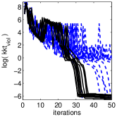
(a) $R=20$

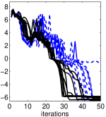
(b) $R=60$

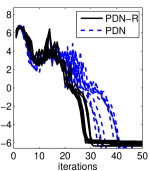
(c) $R=100$

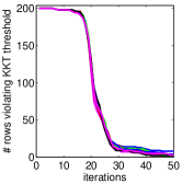
(d) $R=20$

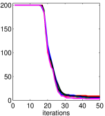
(e) $R=60$

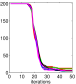
(f) $R=100$

Fig. 2: Convergence behavior of PDN-R (Algorithm 3) and PDN over ten runs with different start points, for three values of $R$. The upper graphs plot $\log(\textrm{kkt}_{\textrm{viol}})$, showing how the maximum violation over all row subproblems varies as the number of iterations increases. Solid lines are PDN-R, dashed lines are PDN. The lower graphs plot the number of rows violating the KKT-based stop tolerance (ten runs of only PDN-R).

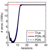
(a) Number of zero entries in ${\bm{\mathbf{{A}}}}^{(1)}$ for $R=100$

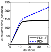
(b) Cumulative execution time for $R=100$

Fig. 3: Additional convergence behavior over ten runs with different start points. Solid lines are PDN-R, dashed lines are PDN. The red horizontal line shows the true number of elements exactly equal to zero.

Figures 2a - 2c show how KKT violations decrease with iteration for three different values of $R$. The subproblem was solved ten times from different randomly chosen start points. (Since the subproblem is strictly convex, there is a single unique minimum that is reached from every start point.) Each solid line plots the maximum $\textrm{kkt}_{\textrm{viol}}$ over all 200 row subproblems for one of the ten PDN-R runs. Each dashed line plots the $\textrm{kkt}_{\textrm{viol}}$ of the block subproblem for one of the ten PDN runs. Note the $y$-axis is the $\log_{10}$ of $\textrm{kkt}_{\textrm{viol}}$. The figure demonstrates that after some initial slow progress, both algorithms exhibit the fast quadratic convergence rate typical of Newton methods. PDN-R clearly takes fewer iterations to compute a factorization with small $\textrm{kkt}_{\textrm{viol}}$.

Figures 2d - 2f show the number of row subproblems in PDN-R that satisfy the KKT-based stop tolerance after a given number of iterations. Remember that all row subproblems must satisfy the KKT tolerance before the algorithm declares a solution.

Figure 3 shows additional features of the convergence, for just the case of $R=100$ components (behavior is similar for other values of $R$). In Figure 3a we see the number of elements of ${\bm{\mathbf{{A}}}}^{(1)}$ exactly equal to zero. Data for this experiment was generated stochastically from sparse factor matrices (see Appendix A); hence, we expect a sparse solution. The plot indicates that sparsity can be achieved after reducing $\textrm{kkt}_{\textrm{viol}}$ to a moderately small tolerance (around $10^{-2}$ in this example). We return to sparsity of the solution in the sections below.

In Figure 3b we see that execution time per iteration decreases when variables are closer to a solution. PDN-R execution time becomes very small because only a few row subproblems need to satisfy the convergence tolerance, and only these are updated. PDN takes more time per iteration because it computes a single search direction for updating all variables in the block subproblem, even when most of the variables are near an optimal value. These experiments show that PDN-R and PDN behave similarly for the convex subproblem and that PDN-R is a little faster; much larger differences appear when the full factorization is computed in Section 4.2.1.

4.1.2 PQN-R and PQN on the Convex Subproblem

In this section we demonstrate the importance of the row subproblem formulation by comparing PQN-R with PQN, showing the huge speedup achieved with our row subproblem formulation. We compare the algorithms on the mode-1 subproblem described above, from the same ten random initial guesses for ${\bm{\mathbf{{A}}}}^{(1)}$. Table 2 lists the average CPU times over ten runs. PQN-R was executed until the $\textrm{kkt}_{\textrm{viol}}$ was less than $\tau=10^{-8}$. PQN was unable to achieve this level of accuracy, so execution was stopped at a tolerance of $10^{-3}$. Results in the table show that PQN-R is much faster at decreasing the KKT violation. We note that a KKT violation of $10^{-8}$ is approximately the square root of machine epsilon, the smallest practical value that can be attained.

Table 2: Convergence comparison in solving the subproblem

	Algorithm PQN		Algorithm PQN-R
$R$	$\textrm{kkt}_{\textrm{viol}}<10^{-1}$	$\textrm{kkt}_{\textrm{viol}}<10^{-3}$	$\textrm{kkt}_{\textrm{viol}}<10^{-1}$	$\textrm{kkt}_{\textrm{viol}}<10^{-8}$
20	625 secs	690 secs	12.4 secs	17.1 secs
40	755 secs	846 secs	10.9 secs	16.4 secs
60	822 secs	920 secs	11.3 secs	16.8 secs
80	1022 secs	1141 secs	13.7 secs	19.5 secs
100	993 secs	1125 secs	13.1 secs	20.2 secs

The two algorithms also differ in how they discover the number of elements in ${\bm{\mathbf{{A}}}}^{(1)}$ equal to zero. Both eventually agree on the number of zero elements, but PQN-R is much faster. Figure 4 shows the progress made by the two algorithms; the behavior of PQN for this quantity is erratic and slow to converge.

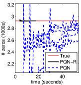
(a) $R=20$

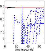
(b) $R=60$

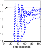
(c) $R=100$

Fig. 4: Number of elements equal to zero in ${\bm{\mathbf{{A}}}}^{(1)}$ found by PQN-R (solid lines, forming a short segment in the upper left) and PQN (dashed lines) as a function of compute time, for a subproblem with different values of $R$. The same subproblem was solved from six different start points, corresponding to the different colors. The red horizontal line shows the true value.

Algorithm PQN might be relatively more competitive for tensor subproblems with a small number of rows. Nevertheless, it is apparent that applying L-BFGS to the block subproblem does not work as well as applying separate instances of L-BFGS to the row subproblems. This is not surprising since the first method ignores the block diagonal structure of the true Hessian. We see no advantages to using PQN and do not consider it further.

4.1.3 PDN-R, PQN-R, and MU on the Convex Subproblem

Next we compare our new row-based algorithms, PDN-R and PQN-R, with the multiplicative update method MU [11]. Again we use the mode-1 subproblem of Section 4.1, from the same ten random initial guesses.

As described in Section 4, MU is a state-of-the-art representative of the most common algorithm for nonnegative tensor factorization. It is a form of scaled steepest-descent with bound constraints [26], and therefore is expected to converge more slowly than Newton or quasi-Newton methods. We see this clearly in Table 3 for two different stop tolerances. The MU algorithm was executed with a time limit of 1800 seconds per problem, and failed to reach $\textrm{kkt}_{\textrm{viol}}<10^{-3}$ before this limit when $R$ was 60 or larger.

Table 3: Time to reach stop tolerance for three algorithms (averaged over ten runs)

	$\textrm{kkt}_{\textrm{viol}}=10^{-2}$			$\textrm{kkt}_{\textrm{viol}}=10^{-3}$
$R$	PDN-R	PQN-R	MU	PDN-R	PQN-R	MU
20	8.1 secs	14.5 secs	97.7 secs	8.1 secs	15.6 secs	161.3 secs
40	25.1 secs	13.1 secs	239.2 secs	25.2 secs	14.6 secs	485.9 secs
60	53.6 secs	13.8 secs	469.2 secs	53.7 secs	15.6 secs	$>$1800 secs
80	92.8 secs	16.3 secs	455.4 secs	92.9 secs	18.1 secs	$>$1800 secs
100	139.8 secs	16.0 secs	730.7 secs	140.0 secs	18.3 secs	$>$1800 secs

Of course, the disparity in convergence time is more pronounced when a smaller KKT error is demanded. Figure 5 shows the decrease in KKT violation as a function of compute time. Here we see that MU makes a faster initial reduction in KKT violation than PDN-R or PQN-R, but then it slows to a linear rate of convergence. Notice the gap from time zero for PDN-R and PQN-R, which reflects setup cost before the first iteration result is computed. For PQN-R the setup time is fairly constant with $R$ (about 3.8 seconds), while PDN-R has a setup time that increases with $R$ (11.5 seconds for $R=100$). Unlike MU, both algorithms must construct software structures for all row subproblems before a first iteration result appears. Figure 5 also reveals that PDN-R is slower relative to PQN-R as the number of components $R$ increases. This is because the cost of solving a Newton-based Hessian is $O(R^{3})$, while the limited-memory BFGS Hessian cost is $O(R)$.

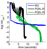
(a) $R=20$

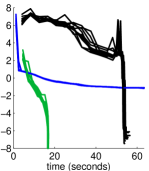
(b) $R=60$

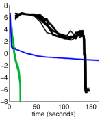
(c) $R=100$

Fig. 5: Convergence behavior comparison on subproblem for different values of $R$ (ten runs each). Algorithm MU (blue) makes fast initial progress in reducing the violation, but slows dramatically after reaching a violation of about 0.1. PDN-R (black) and PQN-R (green) reduce the violation much further, with PQN-R being faster for higher values of $R$.

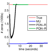
(a) $R=20$

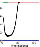
(b) $R=60$

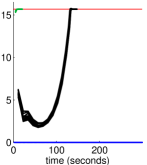
(c) $R=100$

Fig. 6: Effectiveness of the three algorithms in finding a sparse solution for different values of $R$. In each case the number of elements in ${\bm{\mathbf{{A}}}}^{(1)}$ equal to zero is plotted against execution time. The PDN-R (black) and PQN-R (green) algorithms are much faster than MU (blue) at finding the zeros. The horizontal red line shows the true value.

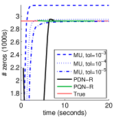
(a) $R=20$

(b) $R=60$

(c) $R=100$

Fig. 7: Comparison of PDN-R, PQN-R and MU in finding elements of ${\bm{\mathbf{{A}}}}^{(1)}$ equal to zero for a sample run. MU rarely finds exact zeros; therefore, we show results of applying various thresholds. Some experimentation may be needed to find the best threshold; regardless, it is slower than the methods proposed here.

Figure 5 indicates that algorithm MU is preferred if a relatively large $\textrm{kkt}_{\textrm{viol}}$ is acceptable. We contend that this is not a good choice if the goal is to find a sparse solution. Figure 6 plots the number of elements that equal zero as a function of CPU time. It shows that PDN-R and PQN-R both converge to the correct number of zeros much faster than MU.

On closer inspection we see that MU is actually making factor elements small, and is just very slow at making them exactly zero. If we choose a small positive threshold instead of zero, then MU might arguably do well at finding a sparse solution. Figure 7 summarizes an investigation of this idea. Three different thresholds are shown: $10^{-3}$, $10^{-4}$, and $10^{-5}$. The first threshold is clearly too large, declaring elements to be “zero” when they never converge to such a value. A threshold of $10^{-4}$ is also too large for $R=20$, though possibly acceptable for $R=40$ and $R=60$. The choice of $10^{-5}$ correctly identifies elements converging to zero, but PDN-R and PQN-R identifies them much faster. We conclude that PDN-R and PQN-R are significantly better at finding a true sparse solution than MU, in terms of robustness (no need to choose an ad-hoc threshold) and computation time (assuming a suitable threshold for MU is known).

4.2 Solving the Full Problem

In this section we move from a convex subproblem to solving the full factorization (4). We generate the same $200\times 300\times 400$ tensor data as in Section 4.1 and now treat all modes as optimization variables. An initial guess is constructed for all three modes in the same manner that ${\bm{\mathbf{{A}}}}^{(1)}$ was initialized in Section 4.1. We generate ten different tensors by changing the random seed used in Algorithm 5 and solve each from a single initial guess. All tensors are factorized from the same initial guess; however, since the full factorization is a nonconvex optimization problem, algorithms may converge to different local solutions.

We expect our local solutions to be reasonably close to the multilinear model $\bm{\mathscr{{M}}}=\llbracket{\bm{\mathbf{{\lambda}}}};{\bm{\mathbf{{A}}}}^{(1)},\dots,{\bm{\mathbf{{A}}}}^{(N)}\rrbracket$ that generated the synthetic tensor data. We compared computed solutions with the original model using the Tensor Toolbox function score with option greedy. This function implements the congruence test described in [37] and [1]. The comparison considers angular differences between corresponding vectors of the factor matrices, producing a number between zero (poor match) and one (exact match). Solutions computed with any algorithm to a tolerance of $\tau=10^{-4}$ scored above 0.84 (see the supplementary material for a detailed breakdown). Perfect scores cannot be seen because the tensor data is generated from the model as a noisy Poisson process. Scores of less than 0.01 resulted when comparing the solution to other models generated with a different random seed. These results show that an accurate factorization can yield good approximations to the original factors for our test problems; however, our focus is on behavior of the algorithms in computing a solution.

4.2.1 Comparing PDN-R with PDN

We first compare the two Newton-based methods: PDN-R, which solves row subproblems for each tensor mode, and PDN, which instead solves the block subproblem as a single matrix. In Section 4.1.1 we saw that the two methods behaved similarly for the convex subproblem of a single tensor mode (except that PDN-R was faster). However, on the full factorization PDN is often unable to make progress from a start point where the KKT violation is large. Sometimes the search direction does not satisfy the sufficient decrease condition of the Armijo line search, even after ten backtracking iterations. More frequently, the line search puts too many variables at the bound of zero, causing the objective function to become undefined in equation (7) because ${\bm{\mathbf{{B}}}}^{(n)}{\bm{\mathbf{{\Pi}}}}^{(n)}$ is zero for elements where ${\bm{\mathbf{{X}}}}_{(n)}$ is nonzero.

If the line search fails in a subproblem, then we compute a multiplicative update step for that iteration to make progress. This allows PDN to reach points where the KKT error is smaller, and we find that subsequent damped Newton steps are successful until convergence. Table 4 quantifies the number of line search failures over the first 20 iterations, beginning from a random start point where $\textrm{kkt}_{\textrm{viol}}$ is typically larger than $10^{3}$. Columns in the table correspond to different values for the initial damping parameter $\mu_{0}$. We expect larger values of $\mu_{k}$ to improve robustness by effectively shortening the step length and hopefully avoiding the mistake of setting too many variables to zero. However, a serious drawback to increasing $\mu_{k}$ is that it damps out Hessian information, which can hinder the convergence rate. The table shows that improvement in robustness is made; however, PDN still suffers from some line search failures. In contrast, PDN-R does not have any line search failures for the same test problems and start points, using the default $\mu_{0}=10^{-5}$.

Table 4: Line search failures by PDN in the first 20 iterations, averaged over five runs. There were up to 900 possible line searches in each case (a maximum of 15 inner iterations per mode, over 20 outer iterations).

$R$	$\mu_{0}=10^{1}$	$\mu_{0}=10^{-2}$	$\mu_{0}=10^{-5}$
20	57.8	88.4	142.2
40	76.2	87.4	164.6
60	59.0	90.8	201.0
80	41.4	82.8	184.6
100	28.8	62.2	168.0

Table 5 shows that PDN-R is significantly faster than PDN even in the region where PDN operates robustly. These runs begin at a start point where $\textrm{kkt}_{\textrm{viol}}<0.1$ and use $\mu_{0}=10^{-2}$ (PDN-R uses its default of $\mu_{0}=10^{-5}$) so that PDN does not suffer any line search failures. Five runs are made for each of the five values of $R$, and the method stops when the algorithm reduces $\textrm{kkt}_{\textrm{viol}}$ below a given threshold (rows of Table 5). PDN does not always reach a threshold value in the three-hour-computation-time limit, but PDN-R always succeeds. The third column shows that the number of outer iterations needed to reach a threshold is very similar between PDN-R and PDN. The fourth column shows that PDN-R executes much faster.

Table 5: Comparison of PDN-R and PDN execution times for various stop tolerances. 25 experiments were run, the algorithms compared for each experiment that PDN completed, and the average value reported. The third column is computed as $|\text{its}_{\text{PDN}}-\text{its}_{\text{PDN-R}}|/\max\{\text{its}_{\text{PDN}},\text{its}_{\text{PDN-R}}\}$. The fourth column shows that PDN-R executes from 8 to 9 times faster than PDN (the column reports average and standard deviation). The last column shows average execution time of PDN-R.

$\textrm{kkt}_{\textrm{viol}}$	PDN failures	avg diff in outer its	PDN-R speedup	PDN-R time
$10^{-2}$	2	2.48 %	$9.1\pm 1.4$	463.3 secs
$10^{-3}$	5	3.02 %	$8.7\pm 1.4$	595.0 secs
$10^{-4}$	9	2.68 %	$8.5\pm 1.7$	609.7 secs
$10^{-5}$	13	7.93 %	$9.5\pm 2.4$	573.1 secs

Iterations of PDN-R run faster because each row subproblem has an individualized step size and damping parameter (this was discussed previously in Section 4.1.1). Given the large disparity in execution time and the lack of robustness when far from a solution, we find no advantages to using PDN and do not consider it further.

4.2.2 Comparing PDN-R, PQN-R, and MU

Table 6 summarizes the time to reach a KKT threshold of $10^{-3}$ for each algorithm over the synthetic data tensors. Like the convex subproblem tested in Section 4.1.3, the PDN-R and PQN-R methods converge to this relatively high accuracy much faster than MU, again showing the value of second-order information. As in the subproblem, we see that PQN-R is faster relative to PDN-R as the number of components, $R$, increases. Figure 8 shows convergence behavior of the full factorization problem in the same way that Figure 5 showed behavior of the convex subproblem. The KKT error of the full problem does not reach the quadratic rate of decrease seen in the subproblem. This is due to nonconvexity of the full factorization problem, and the alternation between solutions of each mode.

Table 6: Time to reach stop tolerance $10^{-3}$ on full problem (over ten runs). Mean and standard deviation are reported. Some runs of MU failed to reach the tolerance in three hours of execution. Results for different stop tolerances are in the supplementary material.

$R$	PDN-R	PQN-R	MU
20	229 $\pm$   57 secs	397 $\pm$ 123 secs	3355 $\pm$ 1933 secs	(0 failures)
40	493 $\pm$ 151 secs	818 $\pm$ 185 secs	8101 $\pm$ 2045 secs	(2 failures)
60	1003 $\pm$ 349 secs	966 $\pm$ 286 secs	9628 $\pm$   978 secs	(5 failures)
80	1682 $\pm$ 642 secs	1639 $\pm$ 390 secs	no successes	(10 failures)
100	2707 $\pm$ 773 secs	1995 $\pm$ 743 secs	no successes	(10 failures)

As with the subproblem, we also observe better convergence by our methods to a sparse solution. Figure 9 shows PDN-R and PQN-R reaching the final count of zero elements much faster than MU. As in Section 4.1.3, we argue that PDN-R and PQN-R are superior when the task is to find a solution with correct sparsity.

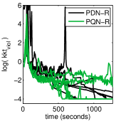
(a) $R=20$

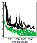
(b) $R=60$

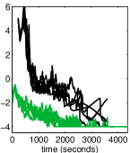
(c) $R=100$

Fig. 8: Convergence behavior of the PDN-R (black lines) and PQN-R (green lines) algorithms in computing a full three-way solution. Each algorithm was run on ten different tensors.

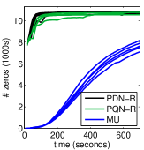
(a) $R=20$

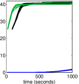
(b) $R=60$

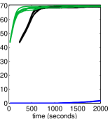
(c) $R=100$

Fig. 9: Effectiveness of the algorithms in finding a sparse solution for a full three-way solution. In each case the total number of elements in ${\bm{\mathbf{{A}}}}^{(1)}$, ${\bm{\mathbf{{A}}}}^{(2)}$, and ${\bm{\mathbf{{A}}}}^{(3)}$ equal to zero is plotted against execution time. The PDN-R (black lines) and PQN-R (green) algorithms are much faster than MU (blue). Each algorithm was run on ten different tensors, so the final number of zero elements has ten different values.

We performed similar experiments on tensors of the same size but different sparsity. Results are in the supplementary material. They lead to the same conclusions as the data in Table 6; namely, that PDN-R and PQN-R are faster than MU, and PQN-R becomes faster than PDN-R as the number of components increases.

The supplementary material also describes a simple experiment with sparse tensors whose factor matrices have a high degree of collinearity between column vectors. Such problems sometimes lead to poor algorithm performance (e.g., the “swamps” in [31]). Performance of PDN-R and PQN-R was much better than algorithm MU in this experiment as well.

4.2.3 Comparing with DBLP Data

We also compare the same three algorithms on the sparse three-way tensor of DBLP data [14] examined in [15]. The data counts the number of papers published by author $i_{1}$ at conference $i_{2}$ in year $i_{3}$, with dimensions $7108\times 1103\times 10$. The tensor contains 112,730 nonzero elements, a density of 0.14%. The data was factorized for $R$ between 10 and 100 in [15] (using a least squares objective function), so we use $R\in\{20,60,100\}$ in our experiments. Behavior of the algorithms on the DBLP data was similar to behavior on our synthetic data. Figure 10 shows how the count of elements equal to zero changes as algorithms progress, for ten runs that start from different random initial guesses. Again we see that PDN-R and PQN-R reach a sparse solution faster than MU.

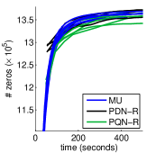
(a) $R=20$

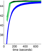
(b) $R=60$

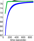
(c) $R=100$

Fig. 10: Effectiveness of the algorithms in finding a sparse solution for the DBLP tensor. In each case the total number of elements in ${\bm{\mathbf{{A}}}}^{(1)}$, ${\bm{\mathbf{{A}}}}^{(2)}$, and ${\bm{\mathbf{{A}}}}^{(3)}$ equal to zero is plotted against execution time. The PDN-R (black lines) and PQN-R (green) algorithms are much faster than MU (blue).

Factorizations of the DBLP data computed with PDN-R and PQN-R were quite sparse, making them easier to interpret. The fraction of elements exactly equal to zero in the computed conference factor matrix was 98.1%. The author factor matrix was also very sparse, with 95.4% of the elements exactly zero. These results were for a factorization with $R=100$, stopped after 800 seconds of execution with the KKT violation reduced to around $5\times 10^{-4}$. Figure 11 shows a component that detects related conferences that took place only in even years. The two dominant conferences are the same as those reported in Figure 7 of [15]. Figure 12 shows another component that groups conferences that took place only in odd years. In both components, the sparsity is striking, especially for the conference factor.

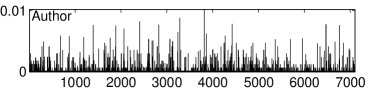
(a)

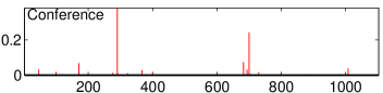
(b)

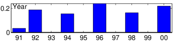
(c)

Fig. 11: Computed factors from DBLP data for component 26 (i.e., the 26th largest component by weight). The two dominant conferences, ECAI and KR, occurred only in even years, except for KR in 1991. Factors are extremely sparse: 91% (6456) of elements in the author factor are exactly zero, as are 98% (1084) of the conference elements.

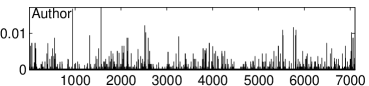
(a)

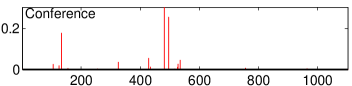
(b)

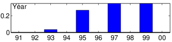
(c)

Fig. 12: Computed factors from DBLP data for component 41. The three dominant conferences (ICDAR, ICIAP, and CAIP) occurred only in odd years. In this component, 93% (6626) of elements in the author factor are exactly zero, as are 98% (1083) conference elements.

5 Summary

In this paper we consider the problem of nonnegative tensor factorization using a K-L objective function, and we derive a row subproblem formulation that allows efficient use of second order information. We present two new algorithms that exploit the row subproblem reformulation: PDN-R uses second derivatives in the optimization, while PQN-R uses a quasi-Newton approximation. We show that using the same second order information in a block subproblem formulation is less robust and more expensive computationally than a row subproblem formulation. We show that both PDN-R and PQN-R are much faster than the best multiplicative update method,especially when high accuracy solutions are desired. We further show that high accuracy is needed to identify zeros and compute sparse factors without resorting to the use of ad-hoc thresholds. This is important because sparse count data is likely to have sparsity in the factors, and sparse factors are always easier to interpret.

Our Matlab algorithms will appear in Version 2.6 of the Tensor Toolbox [4]. We mention in section 2.2 that row subproblems can be solved in parallel, and we anticipate developing other versions of the algorithms for shared and distributed memory machines.

Appendix A Generating Synthetic Test Data

The goal is to create artificial nonnegative factor matrices and use these to compute a data tensor whose elements follow a Poisson distribution with multilinear parameters. Factorizing the data tensor should yield quantities that are close to the original factor matrices. The procedure is based on the work of [11].

The data tensor should be sparse, reflecting Poisson distributions whose probability of zero is not negligible. Each entry is a count of the number of samples assigned to this cell, out of a given total number of samples $S$. We generate factor matrices in each tensor mode and treat them as stochastic quantities to draw the $S$ samples that provide data tensor counts.

Our generation procedure utilizes the function create_problem from Tensor Toolbox for Matlab [4], supplying a custom function for the Factor_Generator parameter (available as Matlab code from the authors). We create a multilinear model, $\bm{\mathscr{{M}}}=[{\bm{\mathbf{{\lambda}}}};{\bm{\mathbf{{A}}}}^{(1)}\ldots{\bm{\mathbf{{A}}}}^{(N)}]$, where ${\bm{\mathbf{{A}}}}^{(n)}\in{\cal R}^{I_{n}\times R}$ and ${\bm{\mathbf{{\lambda}}}}\in{\cal R}^{R}$, and sizes $I_{n}$ and $R$ are given. The model is generated by the following procedure:

Algorithm 5 Generation of Synthetic Sparse Poisson Tensor Data

Given tensor size, $I_{1}\times\cdots\times I_{N}$, number of components, $R$, and number of samples, $S$.
Return a model $\bm{\mathscr{{M}}}=[{\bm{\mathbf{{\lambda}}}};{\bm{\mathbf{{A}}}}^{(1)}\ldots{\bm{\mathbf{{A}}}}^{(N)}]$ and corresponding sparse data tensor $\bm{\mathscr{{X}}}$.

1:In each column of ${\bm{\mathbf{{A}}}}^{(n)}$, choose $20\%$ of the elements at random and set their value to $1+10Rx$, where $x$ is a random value from a uniform distribution on $(0,1)$. Set the other elements equal to the small constant 0.1.

2:Choose random values for elements in ${\bm{\mathbf{{\lambda}}}}$ from a uniform distribution on $(0,1)$.

3:Rescale each column of ${\bm{\mathbf{{A}}}}^{(n)}$ so entries sum to 1, absorbing the scale factor into the corresponding element of ${\bm{\mathbf{{\lambda}}}}$.

4:Rescale the vector ${\bm{\mathbf{{\lambda}}}}$ so entries sum to 1.

5:for $s=1,\dots,S$ do

6:     Treating ${\bm{\mathbf{{\lambda}}}}$ as a distribution, choose a component $r$ at random.

7:     Treating the $r$th column of ${\bm{\mathbf{{A}}}}^{(1)}$ as a distribution, choose an index $i_{1}$ with probability proportional to ${\bm{\mathbf{{a}}}}^{(1)}_{r}$. Do the same for indices $i_{2},\ldots,i_{N}$, resulting in the index i chosen with probability

$$P(\textbf{i})=a^{(1)}_{i_{1}r}a^{(2)}_{i_{2}r}\ldots a^{(N)}_{i_{N}r}.$$

8:     Increment the ith entry of $\bm{\mathscr{{X}}}$ by one.

9:end for

10:Rescale ${\bm{\mathbf{{\lambda}}}}\leftarrow S{\bm{\mathbf{{\lambda}}}}$ so that $\|{\bm{\mathbf{{\lambda}}}}\|_{1}=S$. $\triangleright$ Recall Step 4 sets $\|{\bm{\mathbf{{\lambda}}}}\|_{1}=1$.

Step 1 defines a strong preference for certain values of each index. As $R$ increases, the relative probability of these indices is also increased so that they continue to stand out as strong preferences.

Step 10 rescales ${\bm{\mathbf{{\lambda}}}}$ so that the $\ell_{1}$ norms of the generated data tensor $\bm{\mathscr{{X}}}$ and K-tensor are the same in any mode-$n$ unfolding. For example:

$$\left\|{\bm{\mathbf{{X}}}}_{(1)}\right\|_{1} =\left\|{\bm{\mathbf{{A}}}}^{(1)}{\bm{\mathbf{{\Lambda}}}}({\bm{\mathbf{{A}}}}^{(N)}\odot\ldots\odot{\bm{\mathbf{{A}}}}^{(2)})^{T}\right\|_{1}$$

$$=\sum_{i=1}^{I_{1}}\sum_{r=1}^{R}\lambda_{r}a^{(1)}_{ri}$$

$$=\sum_{r=1}^{R}\lambda_{r}$$

The second equality uses the fact that rows of the Khatri-Rao product sum to one when columns of ${\bm{\mathbf{{A}}}}^{(n)}$ sum to one (see the comments after equation (5)).

Appendix B Supplementary Material

This supplementary section provides detailed results for some experiments mentioned in the paper. Refer to Section 4 of the paper for a description of default parameters used for the algorithms and characteristics of the workstation used for testing.

B.1 Performance on $200\times 1000$ Data Set

Section 1.1 of the paper states that a 2-way tensor of size $200\times 1000$ was too large to factorize by the method of Zdunek and Cichocki [42] but not difficult for our algorithms. Here we support our claim with experimental evidence. Reference [42] does not specify tensor details except that the desired factorization has $R=10$ components. We generated a synthetic data tensor according to the procedure in Appendix A of the paper, modifying Step 1 to boost $9\%$ of the elements to $1+4Rx$, where $x$ is a random number chosen from a uniform distribution on $(0,1)$. We tested $R=10$ and $R=50$ components. We compare algorithms PDN-R and PQN-R using default parameters (see Section 4 for values) over ten instances of synthetic data. Table 7 shows characteristics of the data, and results in Table 8 demonstrate that the problems are solved to high accuracy in under ten minutes.

Table 7: Sparsity of synthetic tensors versus the number of components $R$, for tensors of size $200\times 1000$, generated by boosting $9\%$ of the elements to $1+4Rx$. Number of nonzeros is the average over ten tensors.

$R$	Number Nonzeros	Density
10	50,144	25.1%
50	61,826	30.9%

Table 8: Time to reach various stop tolerances for tensors of size $200\times 1000$. Mean and standard deviation are reported over ten runs. Both methods reach the tolerance of $\tau=10^{-4}$ in well under ten minutes for $R=50$ components.

10 63 ± 26 secs 155 ± 84 secs50 170 ± 31 secs 311 ± 59 secs𝜏superscript102fragments 10fragments 63 plus-or-minus 26 secsfragments 155 plus-or-minus 84 secs50fragments 170 plus-or-minus 31 secsfragments 311 plus-or-minus 59 secs\begin{array}[]{rl}\tau=10^{-2}&\begin{tabular}[]{r|r|r}$R$&\lx@intercol\hfil{PDN-R}\hfil\lx@intercol\vrule\lx@intercol &\lx@intercol\hfil{PQN-R}\hfil\lx@intercol \\ \hline\cr 10&\, \, 63 $\pm$ \, 26 secs&\, 155 $\pm$ \, 84 secs\\ 50&\, 170 $\pm$ \, 31 secs&\, 311 $\pm$ \, 59 secs\\ \end{tabular}\end{array}

RPDN-RPQN-RRPDN-RPQN-R

10 80 ± 25 secs 184 ± 100 secs50 191 ± 26 secs 357 ± 86 secs𝜏superscript103fragments fragments10fragments 80 plus-or-minus 25 secsfragments 184 plus-or-minus 100 secs50fragments 191 plus-or-minus 26 secsfragments 357 plus-or-minus 86 secs\begin{array}[]{rl}\tau=10^{-3}&\begin{tabular}[]{r|r|r}$R$&\lx@intercol\hfil{PDN-R}\hfil\lx@intercol\vrule\lx@intercol &\lx@intercol\hfil{PQN-R}\hfil\lx@intercol \\ \hline\cr 10&\, \, 80 $\pm$ \, 25 secs&\, 184 $\pm$ 100 secs\\ 50&\, 191 $\pm$ \, 26 secs&\, 357 $\pm$ \, 86 secs\\ \end{tabular}\end{array}

RPDN-RPQN-RRPDN-RPQN-R

10 91 ± 25 secs 208 ± 116 secs50 231 ± 59 secs 385 ± 84 secs𝜏superscript104fragments 10fragments 91 plus-or-minus 25 secsfragments 208 plus-or-minus 116 secs50fragments 231 plus-or-minus 59 secsfragments 385 plus-or-minus 84 secs\begin{array}[]{rl}\tau=10^{-4}&\begin{tabular}[]{r|r|r}$R$&\lx@intercol\hfil{PDN-R}\hfil\lx@intercol\vrule\lx@intercol &\lx@intercol\hfil{PQN-R}\hfil\lx@intercol \\ \hline\cr 10&\, \, 91 $\pm$ \, 25 secs&\, 208 $\pm$ 116 secs\\ 50&\, 231 $\pm$ \, 59 secs&\, 385 $\pm$ \, 84 secs\\ \end{tabular}\end{array}

RPDN-RPQN-RRPDN-RPQN-R

B.2 Detail for Results in Section 4.2.2

Section 4.2.2 of the paper contains a table showing the performance of algorithms PDN-R, PQN-R, and MU on a tensor of size $200\times 300\times 400$ for different values of $R$. The table reports execution time for the algorithms to reach a stop tolerance of $\tau=10^{-3}$. Supplementary Tables 9 - 12 contain additional results from the same tests. Table 9 shows that the relative advantage of the algorithms holds for all tolerances; in particular, PDN-R and PQN-R are faster than MU at all tolerances, and PQN-R becomes faster than PDN-R for a sufficiently large number of components. Table 10 shows that the final values of the objective function attained by the three algorithms are nearly identical.

Table 9: Time to reach various stop tolerances ($\tau=10^{-3}$ repeats Table 6 in Section 4.2.2 of the paper). Mean and standard deviation are reported over ten runs. The last column for MU is the number of runs that failed to reach the stop tolerance after three hours (10,800 seconds) of execution.

20 170 ± 37 secs 317 ± 127 secs 997 ± 347 secs (0 failures)40 339 ± 71 secs 573 ± 268 secs3275 ± 1357 secs (0 failures)60 611 ± 126 secs 740 ± 235 secs5758 ± 1275 secs (0 failures)801145 ± 358 secs1340 ± 358 secs9134 ± 1030 secs (1 failure)1001739 ± 359 secs1623 ± 583 secs9687 ± 372 secs (6 failures)𝜏superscript102fragments 20fragments 170 plus-or-minus 37 secsfragments 317 plus-or-minus 127 secsfragments 997 plus-or-minus 347 secs (0 failures)40fragments 339 plus-or-minus 71 secsfragments 573 plus-or-minus 268 secsfragments3275 plus-or-minus 1357 secs (0 failures)60fragments 611 plus-or-minus 126 secsfragments 740 plus-or-minus 235 secsfragments5758 plus-or-minus 1275 secs (0 failures)80fragments1145 plus-or-minus 358 secsfragments1340 plus-or-minus 358 secsfragments9134 plus-or-minus 1030 secs (1 failure)100fragments1739 plus-or-minus 359 secsfragments1623 plus-or-minus 583 secsfragments9687 plus-or-minus 372 secs (6 failures)\begin{array}[]{rl}\tau=10^{-2}&\begin{tabular}[]{r|r|r|rr}$R$&\lx@intercol\hfil{PDN-R}\hfil\lx@intercol\vrule\lx@intercol &\lx@intercol\hfil{PQN-R}\hfil\lx@intercol\vrule\lx@intercol &\lx@intercol\hfil{MU}\hfil\lx@intercol \\ \hline\cr 20&\, 170 $\pm$ \, 37 secs&\, 317 $\pm$ 127 secs&\, 997 $\pm$ \, 347 secs&\, (0 failures)\\ 40&\, 339 $\pm$ \, 71 secs&\, 573 $\pm$ 268 secs&3275 $\pm$ 1357 secs&\, (0 failures)\\ 60&\, 611 $\pm$ 126 secs&\, 740 $\pm$ 235 secs&5758 $\pm$ 1275 secs&\, (0 failures)\\ 80&1145 $\pm$ 358 secs&1340 $\pm$ 358 secs&9134 $\pm$ 1030 secs&\, (1 failure)\\ 100&1739 $\pm$ 359 secs&1623 $\pm$ 583 secs&9687 $\pm$ \, 372 secs&\, (6 failures)\\ \end{tabular}\end{array}

RPDN-RPQN-RMURPDN-RPQN-RMU

20 229 ± 57 secs 397 ± 123 secs3355 ± 1933 secs (0 failures)40 493 ± 151 secs 818 ± 185 secs8101 ± 2045 secs (2 failures)601003 ± 349 secs 966 ± 286 secs9628 ± 978 secs (5 failures)801682 ± 642 secs1639 ± 390 secs-(10 failures)1002707 ± 773 secs1995 ± 743 secs-(10 failures)𝜏superscript103fragments 20fragments 229 plus-or-minus 57 secsfragments 397 plus-or-minus 123 secsfragments3355 plus-or-minus 1933 secs (0 failures)40fragments 493 plus-or-minus 151 secsfragments 818 plus-or-minus 185 secsfragments8101 plus-or-minus 2045 secs (2 failures)60fragments1003 plus-or-minus 349 secsfragments 966 plus-or-minus 286 secsfragments9628 plus-or-minus 978 secs (5 failures)80fragments1682 plus-or-minus 642 secsfragments1639 plus-or-minus 390 secs-(10 failures)100fragments2707 plus-or-minus 773 secsfragments1995 plus-or-minus 743 secs-(10 failures)\begin{array}[]{rl}\tau=10^{-3}&\begin{tabular}[]{r|r|r|rr}$R$&\lx@intercol\hfil{PDN-R}\hfil\lx@intercol\vrule\lx@intercol &\lx@intercol\hfil{PQN-R}\hfil\lx@intercol\vrule\lx@intercol &\lx@intercol\hfil{MU}\hfil\lx@intercol \\ \hline\cr 20&\, 229 $\pm$ \, 57 secs&\, 397 $\pm$ 123 secs&3355 $\pm$ 1933 secs&\, (0 failures)\\ 40&\, 493 $\pm$ 151 secs&\, 818 $\pm$ 185 secs&8101 $\pm$ 2045 secs&\, (2 failures)\\ 60&1003 $\pm$ 349 secs&\, 966 $\pm$ 286 secs&9628 $\pm$ \, 978 secs&\, (5 failures)\\ 80&1682 $\pm$ 642 secs&1639 $\pm$ 390 secs&-&(10 failures)\\ 100&2707 $\pm$ 773 secs&1995 $\pm$ 743 secs&-&(10 failures)\\ \end{tabular}\end{array}

RPDN-RPQN-RMURPDN-RPQN-RMU

20 270 ± 67 secs 451 ± 108 secs5207 ± 1975 secs (1 failure)40 756 ± 383 secs 905 ± 171 secs-(10 failures)601166 ± 390 secs1102 ± 305 secs-(10 failures)801890 ± 617 secs1859 ± 413 secs-(10 failures)1002834 ± 741 secs2280 ± 808 secs-(10 failures)𝜏superscript104fragments 20fragments 270 plus-or-minus 67 secsfragments 451 plus-or-minus 108 secsfragments5207 plus-or-minus 1975 secs (1 failure)40fragments 756 plus-or-minus 383 secsfragments 905 plus-or-minus 171 secs-(10 failures)60fragments1166 plus-or-minus 390 secsfragments1102 plus-or-minus 305 secs-(10 failures)80fragments1890 plus-or-minus 617 secsfragments1859 plus-or-minus 413 secs-(10 failures)100fragments2834 plus-or-minus 741 secsfragments2280 plus-or-minus 808 secs-(10 failures)\begin{array}[]{rl}\tau=10^{-4}&\begin{tabular}[]{r|r|r|rr}$R$&\lx@intercol\hfil{PDN-R}\hfil\lx@intercol\vrule\lx@intercol &\lx@intercol\hfil{PQN-R}\hfil\lx@intercol\vrule\lx@intercol &\lx@intercol\hfil{MU}\hfil\lx@intercol \\ \hline\cr 20&\, 270 $\pm$ \, 67 secs&\, 451 $\pm$ 108 secs&5207 $\pm$ 1975 secs&\, (1 failure)\\ 40&\, 756 $\pm$ 383 secs&\, 905 $\pm$ 171 secs&-&(10 failures)\\ 60&1166 $\pm$ 390 secs&1102 $\pm$ 305 secs&-&(10 failures)\\ 80&1890 $\pm$ 617 secs&1859 $\pm$ 413 secs&-&(10 failures)\\ 100&2834 $\pm$ 741 secs&2280 $\pm$ 808 secs&-&(10 failures)\\ \end{tabular}\end{array}

RPDN-RPQN-RMURPDN-RPQN-RMU

Table 10: Final objective function values reached by the algorithms. Algorithms minimize K-L divergence, but the negative of K-L is shown because this equals the (unnormalized) maximum likelihood. Mean and maximum (most optimal) values are reported over ten runs. Values are in units of $10^{6}$; for example, the average unnormalized log likelihood reached by algorithm PDN-R for $R=20$ was $1.146\times 10^{6}$. The likelihood increases with the number of components because this allows for a better fit to the data.

	PDN-R		PQN-R		MU
$R$	mean	max	mean	max	mean	max
20	1.146	1.205	1.144	1.193	1.145	1.193
40	1.448	1.475	1.448	1.475	1.447	1.473
60	1.610	1.643	1.611	1.647	1.610	1.640
80	1.716	1.735	1.715	1.734	1.715	1.738
100	1.794	1.811	1.794	1.810	1.794	1.811

Tables 11 and 12 report the agreement between the models computed by each algorithm and the factor matrices from which tensor data was generated (the “true model”). Agreement is measured by the Tensor Toolbox score function, which implements the method described in [1]. The score considers the angles between all factor matrix column vectors. Let the two $R$-component models for a three-way tensor have weight vectors and factor matrices $\{{\bm{\mathbf{{\lambda}}}}^{A},{\bm{\mathbf{{A}}}}^{(1)},{\bm{\mathbf{{A}}}}^{(2)},{\bm{\mathbf{{A}}}}^{(3)}\}$ and $\{{\bm{\mathbf{{\lambda}}}}^{B},{\bm{\mathbf{{B}}}}^{(1)},{\bm{\mathbf{{B}}}}^{(2)},{\bm{\mathbf{{B}}}}^{(3)}\}$. Assume columns of factor matrices are normalized to one in the $\ell_{2}$ norm, adjusting the weights as needed. The comparison is computed from

$$s=\frac{1}{R}\sum_{r=1}^{R}[({\bm{\mathbf{{a}}}}^{(1)}_{r})^{T}{\bm{\mathbf{{b}}}}^{(1)}_{r}][({\bm{\mathbf{{a}}}}^{(2)}_{r})^{T}{\bm{\mathbf{{b}}}}^{(2)}_{r}][({\bm{\mathbf{{a}}}}^{(3)}_{r})^{T}{\bm{\mathbf{{b}}}}^{(3)}_{r}].$$ (23)

The score is the largest $s$ over column permutations of the models. Ideally, $s$ is computed for all possible permutations, but this is not feasible when $R$ is large. Instead, we use the greedy option to limit the number of permutations considered. The score is a number between zero and one, with one indicating a perfect match between the two models.

Table 11 shows that all three algorithms produce solutions with scores in the range of $[0.84,0.92]$, with no clear superiority for any algorithm. To give a sense of score magnitudes, the table also reports the score between computed solutions and factor matrices used to generate other models. The generation procedure in Appendix A is based on random values, so we expect poor scores between a solution and random factor matrices. This is indeed the case, with no scores greater than 0.01. Table 12 reports the score for computed solutions when the algorithm is initialized with the factor matrices of the true model. The solution should be a local minimum close to the true model, representing an easily found solution that gives one of the best possible fits to the data. Since tensor data is generated with statistical noise, a perfect fit is not seen. These “ideal” scores are slightly higher than the scores from algorithm solutions in Table 11.

We notice that scores in Table 12 decrease as $R$ increases. This is because the tensor data has about the same number of samples in each test case (see Table 13), but a model with more components has more variables. As the ratio of data samples to model variables decreases, the variables are affected more strongly by noise in the data, leading to solutions with a lower score.

Table 11: Comparison of final computed solutions with the true model from which data was generated. The comparison uses the Tensor Toolbox score function, executed with option greedy. The score is a number between zero (poor match) and one (exact match). The true model column shows the lowest (worst) score obtained over ten runs when the computed solution is scored against the true model. For comparison, the others column shows the highest (best) score between the computed solution and any of the nine other models, again averaged over ten runs.

	PDN-R		PQN-R		MU
$R$	true model	others	true model	others	true model	others
20	0.919	0.009	0.845	0.009	0.854	0.009
40	0.880	0.010	0.888	0.010	0.892	0.010
60	0.846	0.010	0.873	0.010	0.844	0.010
80	0.876	0.010	0.873	0.010	0.889	0.010
100	0.865	0.010	0.864	0.010	0.847	0.010

Table 12: Comparison of final computed solutions with the true model from which data was generated using the Tensor Toolbox score function. The PDN-R algorithm was initialized with the factor matrices of Appendix A that generated the test data. Columns in the table show the highest (best) and lowest (worst) scores obtained over ten runs.

	PDN-R
$R$	best score	worst score
20	0.996	0.961
40	0.989	0.964
60	0.982	0.913
80	0.965	0.937
100	0.952	0.907

B.3 Section 4.2.2 Repeated with Different Sparsity

The data tensor of Section 4.2.2 was generated by the method described in Step 1 of Appendix A with $20\%$ of element values boosted to $1+10Rx$. In this section, we report on convergence of the algorithms for tensors of the same size but different sparsity. Sparsity was modified by boosting different numbers of elements. The boosting procedure provides tensor data with appropriate Poisson distributions but does not give exact control over the number of nonzeros. We select boost parameters that yield approximately the same number of nonzeros for $R\in\{20,40,60,80,100\}$ so we can more easily compare algorithm performance as a function of $R$. Tables 13 - 15 describe the sparsity of the different test tensors.

Table 13: Sparsity of synthetic tensors versus the number of components $R$, for tensors of size $200\times 300\times 400$, generated by boosting $20\%$ of the elements to $1+10Rx$. Number of nonzeros is the average over ten tensors. (This table repeats Table 1 from the paper.)

$R$	Number Nonzeros	Density
20	413,458	1.72%
40	450,756	1.88%
60	464,443	1.94%
80	470,950	1.96%
100	475,455	1.98%

Table 14: Sparsity of synthetic tensors versus the number of components $R$, for tensors of size $200\times 300\times 400$, generated by boosting $5\%$ of the elements to $1+2Rx$. Number of nonzeros is the average over ten tensors.

$R$	Number Nonzeros	Density
20	158,616	0.66%
40	141,778	0.59%
60	148,273	0.62%
80	161,212	0.67%
100	177,060	0.74%

Table 15: Sparsity of synthetic tensors versus the number of components $R$, for tensors of size $200\times 300\times 400$, generated by boosting $3\%$ of the elements to $1+10Rx$. Number of nonzeros is the average over ten tensors.

$R$	Number Nonzeros	Density
20	55,471	0.23%
40	44,862	0.19%
60	47,171	0.20%
80	51,827	0.22%
100	57,700	0.24%

The experiments in Section 4.2.2 were performed for each of these tensors. Supplementary Table 9 in the previous section shows algorithm performance for the sparse tensor of Table 13 ($20\%$ boost). The tables below show performance for the $5\%$ and $3\%$ boosted tensors. We see that the conclusions from Section 4.2.2 hold for these cases as well: PDN-R and PQN-R are faster than MU in nearly every case, and PQN-R becomes faster than PDN-R for sufficiently large $R$. Comparing the three tables with each other, we see that performance improves when the number of nonzeros in the data decreases.

Table 16: Time to reach various stop tolerances $\tau$ on the tensor with the sparsity in supplementary Table 14 resulting from $5\%$ boost. Mean and standard deviation are reported over ten runs. The last column for MU is the number of runs that failed to reach the stop tolerance after three hours of execution.

20 165 ± 40 secs 353 ± 137 secs 345 ± 214 secs40 393 ± 125 secs 454 ± 148 secs 541 ± 129 secs60 516 ± 124 secs 394 ± 103 secs 865 ± 186 secs80 558 ± 48 secs 386 ± 53 secs1235 ± 210 secs100 658 ± 59 secs 343 ± 44 secs1633 ± 228 secs𝜏superscript102fragments 20fragments 165 plus-or-minus 40 secsfragments 353 plus-or-minus 137 secsfragments 345 plus-or-minus 214 secs40fragments 393 plus-or-minus 125 secsfragments 454 plus-or-minus 148 secsfragments 541 plus-or-minus 129 secs60fragments 516 plus-or-minus 124 secsfragments 394 plus-or-minus 103 secsfragments 865 plus-or-minus 186 secs80fragments 558 plus-or-minus 48 secsfragments 386 plus-or-minus 53 secsfragments1235 plus-or-minus 210 secs100fragments 658 plus-or-minus 59 secsfragments 343 plus-or-minus 44 secsfragments1633 plus-or-minus 228 secs\begin{array}[]{rl}\tau=10^{-2}&\begin{tabular}[]{r|r|r|r}$R$&\lx@intercol\hfil{PDN-R}\hfil\lx@intercol\vrule\lx@intercol &\lx@intercol\hfil{PQN-R}\hfil\lx@intercol\vrule\lx@intercol &\lx@intercol\hfil{MU}\hfil\lx@intercol \\ \hline\cr 20&\, 165 $\pm$ \, 40 secs&\, 353 $\pm$ 137 secs&\, 345 $\pm$ 214 secs\\ 40&\, 393 $\pm$ 125 secs&\, 454 $\pm$ 148 secs&\, 541 $\pm$ 129 secs\\ 60&\, 516 $\pm$ 124 secs&\, 394 $\pm$ 103 secs&\, 865 $\pm$ 186 secs\\ 80&\, 558 $\pm$ \, 48 secs&\, 386 $\pm$ \, 53 secs&1235 $\pm$ 210 secs\\ 100&\, 658 $\pm$ \, 59 secs&\, 343 $\pm$ \, 44 secs&1633 $\pm$ 228 secs\\ \end{tabular}\end{array}

RPDN-RPQN-RMURPDN-RPQN-RMU

20 270 ± 139 secs 580 ± 323 secs no successes40 444 ± 145 secs 509 ± 147 secs no successes60 623 ± 128 secs 475 ± 135 secs no successes80 726 ± 130 secs 487 ± 46 secs no successes100 893 ± 150 secs 442 ± 86 secs no successes𝜏superscript103fragments 20fragments 270 plus-or-minus 139 secsfragments 580 plus-or-minus 323 secs no successes40fragments 444 plus-or-minus 145 secsfragments 509 plus-or-minus 147 secs no successes60fragments 623 plus-or-minus 128 secsfragments 475 plus-or-minus 135 secs no successes80fragments 726 plus-or-minus 130 secsfragments 487 plus-or-minus 46 secs no successes100fragments 893 plus-or-minus 150 secsfragments 442 plus-or-minus 86 secs no successes\begin{array}[]{rl}\tau=10^{-3}&\begin{tabular}[]{r|r|r|r}$R$&\lx@intercol\hfil{PDN-R}\hfil\lx@intercol\vrule\lx@intercol &\lx@intercol\hfil{PQN-R}\hfil\lx@intercol\vrule\lx@intercol &\lx@intercol\hfil{MU}\hfil\lx@intercol \\ \hline\cr 20&\, 270 $\pm$ 139 secs&\, 580 $\pm$ 323 secs&\,\,\, no successes\\ 40&\, 444 $\pm$ 145 secs&\, 509 $\pm$ 147 secs&\,\,\, no successes\\ 60&\, 623 $\pm$ 128 secs&\, 475 $\pm$ 135 secs&\,\,\, no successes\\ 80&\, 726 $\pm$ 130 secs&\, 487 $\pm$ \, 46 secs&\,\,\, no successes\\ 100&\, 893 $\pm$ 150 secs&\, 442 $\pm$ \, 86 secs&\,\,\, no successes\\ \end{tabular}\end{array}

RPDN-RPQN-RMURPDN-RPQN-RMU

20 287 ± 139 secs 585 ± 320 secs no successes40 456 ± 142 secs 526 ± 146 secs no successes60 700 ± 199 secs 566 ± 193 secs no successes80 810 ± 214 secs 662 ± 119 secs no successes100 964 ± 173 secs 631 ± 187 secs no successes𝜏superscript104fragments 20fragments 287 plus-or-minus 139 secsfragments 585 plus-or-minus 320 secs no successes40fragments 456 plus-or-minus 142 secsfragments 526 plus-or-minus 146 secs no successes60fragments 700 plus-or-minus 199 secsfragments 566 plus-or-minus 193 secs no successes80fragments 810 plus-or-minus 214 secsfragments 662 plus-or-minus 119 secs no successes100fragments 964 plus-or-minus 173 secsfragments 631 plus-or-minus 187 secs no successes\begin{array}[]{rl}\tau=10^{-4}&\begin{tabular}[]{r|r|r|r}$R$&\lx@intercol\hfil{PDN-R}\hfil\lx@intercol\vrule\lx@intercol &\lx@intercol\hfil{PQN-R}\hfil\lx@intercol\vrule\lx@intercol &\lx@intercol\hfil{MU}\hfil\lx@intercol \\ \hline\cr 20&\, 287 $\pm$ 139 secs&\, 585 $\pm$ 320 secs&\,\,\, no successes\\ 40&\, 456 $\pm$ 142 secs&\, 526 $\pm$ 146 secs&\,\,\, no successes\\ 60&\, 700 $\pm$ 199 secs&\, 566 $\pm$ 193 secs&\,\,\, no successes\\ 80&\, 810 $\pm$ 214 secs&\, 662 $\pm$ 119 secs&\,\,\, no successes\\ 100&\, 964 $\pm$ 173 secs&\, 631 $\pm$ 187 secs&\,\,\, no successes\\ \end{tabular}\end{array}

RPDN-RPQN-RMURPDN-RPQN-RMU

Table 17: Time to reach various stop tolerances $\tau$ on the tensor with with the sparsity in supplementary Table 15 resulting from $3\%$ boost. Mean and standard deviation are reported over ten runs. The last column for MU is the number of runs that failed to reach the stop tolerance after three hours of execution.

20 143 ± 75 secs 182 ± 73 secs 108 ± 34 secs(0 failures)40 141 ± 19 secs 134 ± 53 secs 143 ± 49 secs(0 failures)60 174 ± 29 secs 114 ± 23 secs 218 ± 46 secs(0 failures)80 219 ± 30 secs 114 ± 20 secs 347 ± 69 secs(0 failures)100 230 ± 35 secs 166 ± 37 secs 481 ± 86 secs(0 failures)𝜏superscript102fragments 20fragments 143 plus-or-minus 75 secsfragments 182 plus-or-minus 73 secsfragments 108 plus-or-minus 34 secs(0 failures)40fragments 141 plus-or-minus 19 secsfragments 134 plus-or-minus 53 secsfragments 143 plus-or-minus 49 secs(0 failures)60fragments 174 plus-or-minus 29 secsfragments 114 plus-or-minus 23 secsfragments 218 plus-or-minus 46 secs(0 failures)80fragments 219 plus-or-minus 30 secsfragments 114 plus-or-minus 20 secsfragments 347 plus-or-minus 69 secs(0 failures)100fragments 230 plus-or-minus 35 secsfragments 166 plus-or-minus 37 secsfragments 481 plus-or-minus 86 secs(0 failures)\begin{array}[]{rl}\tau=10^{-2}&\begin{tabular}[]{r|r|r|rr}$R$&\lx@intercol\hfil{PDN-R}\hfil\lx@intercol\vrule\lx@intercol &\lx@intercol\hfil{PQN-R}\hfil\lx@intercol\vrule\lx@intercol &\lx@intercol\hfil{MU}\hfil\lx@intercol \\ \hline\cr 20&\, 143 $\pm$ \, 75 secs&\, 182 $\pm$ \, 73 secs&\, 108 $\pm$ \, 34 secs&(0 failures)\\ 40&\, 141 $\pm$ \, 19 secs&\, 134 $\pm$ \, 53 secs&\, 143 $\pm$ \, 49 secs&(0 failures)\\ 60&\, 174 $\pm$ \, 29 secs&\, 114 $\pm$ \, 23 secs&\, 218 $\pm$ \, 46 secs&(0 failures)\\ 80&\, 219 $\pm$ \, 30 secs&\, 114 $\pm$ \, 20 secs&\, 347 $\pm$ \, 69 secs&(0 failures)\\ 100&\, 230 $\pm$ \, 35 secs&\, 166 $\pm$ \, 37 secs&\, 481 $\pm$ \, 86 secs&(0 failures)\\ \end{tabular}\end{array}

RPDN-RPQN-RMURPDN-RPQN-RMU

20 172 ± 80 secs 208 ± 77 secs 278 ± 135 secs(0 failures)40 169 ± 40 secs 151 ± 41 secs 363 ± 226 secs(0 failures)60 328 ± 122 secs 139 ± 37 secs 552 ± 229 secs(0 failures)80 290 ± 70 secs 135 ± 21 secs 897 ± 302 secs(0 failures)100 302 ± 84 secs 190 ± 55 secs1320 ± 397 secs(0 failures)𝜏superscript103fragments 20fragments 172 plus-or-minus 80 secsfragments 208 plus-or-minus 77 secsfragments 278 plus-or-minus 135 secs(0 failures)40fragments 169 plus-or-minus 40 secsfragments 151 plus-or-minus 41 secsfragments 363 plus-or-minus 226 secs(0 failures)60fragments 328 plus-or-minus 122 secsfragments 139 plus-or-minus 37 secsfragments 552 plus-or-minus 229 secs(0 failures)80fragments 290 plus-or-minus 70 secsfragments 135 plus-or-minus 21 secsfragments 897 plus-or-minus 302 secs(0 failures)100fragments 302 plus-or-minus 84 secsfragments 190 plus-or-minus 55 secsfragments1320 plus-or-minus 397 secs(0 failures)\begin{array}[]{rl}\tau=10^{-3}&\begin{tabular}[]{r|r|r|rr}$R$&\lx@intercol\hfil{PDN-R}\hfil\lx@intercol\vrule\lx@intercol &\lx@intercol\hfil{PQN-R}\hfil\lx@intercol\vrule\lx@intercol &\lx@intercol\hfil{MU}\hfil\lx@intercol \\ \hline\cr 20&\, 172 $\pm$ \, 80 secs&\, 208 $\pm$ \, 77 secs&\, 278 $\pm$ 135 secs&(0 failures)\\ 40&\, 169 $\pm$ \, 40 secs&\, 151 $\pm$ \, 41 secs&\, 363 $\pm$ 226 secs&(0 failures)\\ 60&\, 328 $\pm$ 122 secs&\, 139 $\pm$ \, 37 secs&\, 552 $\pm$ 229 secs&(0 failures)\\ 80&\, 290 $\pm$ \, 70 secs&\, 135 $\pm$ \, 21 secs&\, 897 $\pm$ 302 secs&(0 failures)\\ 100&\, 302 $\pm$ \, 84 secs&\, 190 $\pm$ \, 55 secs&1320 $\pm$ 397 secs&(0 failures)\\ \end{tabular}\end{array}

RPDN-RPQN-RMURPDN-RPQN-RMU

20 178 ± 80 secs 213 ± 76 secs -(10 failures)40 237 ± 188 secs 159 ± 39 secs -(10 failures)60 342 ± 127 secs 176 ± 65 secs -(10 failures)80 290 ± 70 secs 189 ± 94 secs -(10 failures)100 321 ± 98 secs 259 ± 129 secs -(10 failures)𝜏superscript104fragments fragments20fragments 178 plus-or-minus 80 secsfragments 213 plus-or-minus 76 secs -(10 failures)40fragments 237 plus-or-minus 188 secsfragments 159 plus-or-minus 39 secs -(10 failures)60fragments 342 plus-or-minus 127 secsfragments 176 plus-or-minus 65 secs -(10 failures)80fragments 290 plus-or-minus 70 secsfragments 189 plus-or-minus 94 secs -(10 failures)100fragments 321 plus-or-minus 98 secsfragments 259 plus-or-minus 129 secs -(10 failures)\begin{array}[]{rl}\tau=10^{-4}&\begin{tabular}[]{r|r|r|rr}$R$&\lx@intercol\hfil{PDN-R}\hfil\lx@intercol\vrule\lx@intercol &\lx@intercol\hfil{PQN-R}\hfil\lx@intercol\vrule\lx@intercol &\lx@intercol\hfil{MU}\hfil\lx@intercol \\ \hline\cr 20&\, 178 $\pm$ \, 80 secs&\, 213 $\pm$ \, 76 secs&\qquad\,\, -&(10 failures)\\ 40&\, 237 $\pm$ 188 secs&\, 159 $\pm$ \, 39 secs&\qquad\,\, -&(10 failures)\\ 60&\, 342 $\pm$ 127 secs&\, 176 $\pm$ \, 65 secs&\qquad\,\, -&(10 failures)\\ 80&\, 290 $\pm$ \, 70 secs&\, 189 $\pm$ \, 94 secs&\qquad\,\, -&(10 failures)\\ 100&\, 321 $\pm$ \, 98 secs&\, 259 $\pm$ 129 secs&\qquad\,\, -&(10 failures)\\ \end{tabular}\end{array}

RPDN-RPQN-RMURPDN-RPQN-RMU

B.4 Collinear Factor Matrices

Tensor data in these experiments was designed to reflect underlying factor matrices that have nearly collinear columns. Algorithms PDN-R and PQN-R do much better than MU in these experiments. The basic idea, proposed in Phan et al. [33], is to generate random factor matrices and then modify column vectors according to

$${\bm{\mathbf{{a}}}}^{(n)}_{r}={\bm{\mathbf{{a}}}}^{(n)}_{1}+\alpha{\bm{\mathbf{{a}}}}^{(n)}_{r}\quad\mbox{for}\;\;r\in 2,\ldots,R,$$ (24)

with $\alpha=0.5$. We generated synthetic data according to Appendix A but added the collinearity modification after Step 1.

The modification significantly impacts the sparsity of the generated tensor, adding many nonzero elements because the boosted elements in column $r=1$ become boosted elements in all other columns. This makes it difficult to compare performance “before” and “after” the collinearity modification. Instead, we made two experiments with different values of $\alpha$ and view them as two different results.

Collinearity is measured as the cosine between pairs of column vectors. For real-valued $N$-vectors ${\bm{\mathbf{{x}}}}$ and ${\bm{\mathbf{{y}}}}$,

$$\mbox{cos}({\bm{\mathbf{{x}}}},{\bm{\mathbf{{y}}}})=\frac{{\bm{\mathbf{{x}}}}^{T}{\bm{\mathbf{{y}}}}}{\|{\bm{\mathbf{{x}}}}\|\|{\bm{\mathbf{{y}}}}\|}\;.$$

If elements of ${\bm{\mathbf{{x}}}}$ and ${\bm{\mathbf{{y}}}}$ are independent random variables chosen from a uniform distribution on $(0,1)$, then the expected value of their cosine is 0.75. However, the sparse columns generated by Appendix A are not uniform. For instance, average collinearity among column pairs in the experiments of supplementary Section B.2 is close to $0.10$.

Tables 18 - 21 show tensor characteristics and computational performance for two experiments. The tensors in the experiments have the same size but use a different value of $\alpha$ in equation (24) to modify collinearity, which also changes their sparsity; hence, the two experiments should not be compared with each other. What they each show is that algorithms PDN-R and PQN-R are much faster than MU, especially when high accuracy is desired.

Table 18: Sparsity and collinearity of synthetic tensors versus the number of components $R$, for tensors of size $50\times 50\times 50$, generated by boosting $10\%$ of the elements to $1+10Rx$, and modifying collinearity using $\alpha=0.5$ in equation (24). All Pairs shows the average collinearity between all pairs of column vectors within each factor matrix. Data under ${\bm{\mathbf{{a}}}}_{1}$ Pairs shows the average collinearity between the ${\bm{\mathbf{{a}}}}^{(n)}_{1}$ column vector and all others within each factor matrix. All measurements are an average over ten tensors.

	Sparsity		Collinearity
$R$	Number Nonzeros	Density	All Pairs	${\bm{\mathbf{{a}}}}_{1}$ Pairs
10	16,442	13.2%	0.839	0.900
20	14,908	11.9%	0.828	0.897
30	15,572	12.5%	0.830	0.900
40	16,892	13.5%	0.800	0.882

Table 19: Time to reach various stop tolerances $\tau$ on tensors of size $50\times 50\times 50$, generated by boosting $10\%$ of the elements to $1+10Rx$, and modifying collinearity using $\alpha=0.5$ in equation (24). Mean and standard deviation are reported over ten runs. The last column for MU is the number of runs that failed to reach the stop tolerance after 1000 seconds of execution.

10 9 ± 3 secs 14 ± 3 secs 26 ± 7 secs (0 failures)20 18 ± 7 secs 23 ± 6 secs 75 ± 35 secs (0 failures)30 20 ± 5 secs 35 ± 14 secs 97 ± 36 secs (0 failures)40 28 ± 6 secs 46 ± 17 secs191 ± 84 secs (0 failures)𝜏superscript102fragments 10fragments 9 plus-or-minus 3 secsfragments 14 plus-or-minus 3 secsfragments 26 plus-or-minus 7 secs (0 failures)20fragments 18 plus-or-minus 7 secsfragments 23 plus-or-minus 6 secsfragments 75 plus-or-minus 35 secs (0 failures)30fragments 20 plus-or-minus 5 secsfragments 35 plus-or-minus 14 secsfragments 97 plus-or-minus 36 secs (0 failures)40fragments 28 plus-or-minus 6 secsfragments 46 plus-or-minus 17 secsfragments191 plus-or-minus 84 secs (0 failures)\begin{array}[]{rl}\tau=10^{-2}&\begin{tabular}[]{r|r|r|rr}$R$&\lx@intercol\hfil{PDN-R}\hfil\lx@intercol\vrule\lx@intercol &\lx@intercol\hfil{PQN-R}\hfil\lx@intercol\vrule\lx@intercol &\lx@intercol\hfil{MU}\hfil\lx@intercol \\ \hline\cr 10&\, \, \, 9 $\pm$ \, \, 3 secs&\, 14 $\pm$ \, \, 3 secs&\, 26 $\pm$ \, \, 7 secs&\, (0 failures)\\ 20&\, \, 18 $\pm$ \, \, 7 secs&\, 23 $\pm$ \, \, 6 secs&\, 75 $\pm$ \, 35 secs&\, (0 failures)\\ 30&\, \, 20 $\pm$ \, \, 5 secs&\, 35 $\pm$ \, 14 secs&\, 97 $\pm$ \, 36 secs&\, (0 failures)\\ 40&\, \, 28 $\pm$ \, \, 6 secs&\, 46 $\pm$ \, 17 secs&191 $\pm$ \, 84 secs&\, (0 failures)\\ \end{tabular}\end{array}

RPDN-RPQN-RMURPDN-RPQN-RMU

10 20 ± 11 secs 16 ± 4 secs223 ± 126 secs (0 failures)20 25 ± 11 secs 25 ± 6 secs511 ± 191 secs (1 failure)30 25 ± 6 secs 38 ± 16 secs719 ± 117 secs (2 failures)40 35 ± 7 secs 59 ± 26 secs734 ± 172 secs (4 failures)𝜏superscript103fragments 10fragments 20 plus-or-minus 11 secsfragments 16 plus-or-minus 4 secsfragments223 plus-or-minus 126 secs (0 failures)20fragments 25 plus-or-minus 11 secsfragments 25 plus-or-minus 6 secsfragments511 plus-or-minus 191 secs (1 failure)30fragments 25 plus-or-minus 6 secsfragments 38 plus-or-minus 16 secsfragments719 plus-or-minus 117 secs (2 failures)40fragments 35 plus-or-minus 7 secsfragments 59 plus-or-minus 26 secsfragments734 plus-or-minus 172 secs (4 failures)\begin{array}[]{rl}\tau=10^{-3}&\begin{tabular}[]{r|r|r|rr}$R$&\lx@intercol\hfil{PDN-R}\hfil\lx@intercol\vrule\lx@intercol &\lx@intercol\hfil{PQN-R}\hfil\lx@intercol\vrule\lx@intercol &\lx@intercol\hfil{MU}\hfil\lx@intercol \\ \hline\cr 10&\, \, 20 $\pm$ \, 11 secs&\, 16 $\pm$ \, \, 4 secs&223 $\pm$ 126 secs&\, (0 failures)\\ 20&\, \, 25 $\pm$ \, 11 secs&\, 25 $\pm$ \, \, 6 secs&511 $\pm$ 191 secs&\, (1 failure)\\ 30&\, \, 25 $\pm$ \, \, 6 secs&\, 38 $\pm$ \, 16 secs&719 $\pm$ 117 secs&\, (2 failures)\\ 40&\, \, 35 $\pm$ \, \, 7 secs&\, 59 $\pm$ \, 26 secs&734 $\pm$ 172 secs&\, (4 failures)\\ \end{tabular}\end{array}

RPDN-RPQN-RMURPDN-RPQN-RMU

10 32 ± 17 secs 17 ± 5 secs295 ± 113 secs (1 failure)20 28 ± 12 secs 26 ± 6 secs784 ± 221 secs (8 failures)30 28 ± 6 secs 40 ± 17 secs-(10 failures)40 46 ± 21 secs 63 ± 26 secs-(10 failures)𝜏superscript104fragments 10fragments 32 plus-or-minus 17 secsfragments 17 plus-or-minus 5 secsfragments295 plus-or-minus 113 secs (1 failure)20fragments 28 plus-or-minus 12 secsfragments 26 plus-or-minus 6 secsfragments784 plus-or-minus 221 secs (8 failures)30fragments 28 plus-or-minus 6 secsfragments 40 plus-or-minus 17 secs-(10 failures)40fragments 46 plus-or-minus 21 secsfragments 63 plus-or-minus 26 secs-(10 failures)\begin{array}[]{rl}\tau=10^{-4}&\begin{tabular}[]{r|r|r|rr}$R$&\lx@intercol\hfil{PDN-R}\hfil\lx@intercol\vrule\lx@intercol &\lx@intercol\hfil{PQN-R}\hfil\lx@intercol\vrule\lx@intercol &\lx@intercol\hfil{MU}\hfil\lx@intercol \\ \hline\cr 10&\, \, 32 $\pm$ \, 17 secs&\, 17 $\pm$ \, \, 5 secs&295 $\pm$ 113 secs&\, (1 failure)\\ 20&\, \, 28 $\pm$ \, 12 secs&\, 26 $\pm$ \, \, 6 secs&784 $\pm$ 221 secs&\, (8 failures)\\ 30&\, \, 28 $\pm$ \, \, 6 secs&\, 40 $\pm$ \, 17 secs&-&(10 failures)\\ 40&\, \, 46 $\pm$ \, 21 secs&\, 63 $\pm$ \, 26 secs&-&(10 failures)\\ \end{tabular}\end{array}

RPDN-RPQN-RMURPDN-RPQN-RMU

Table 20: Sparsity and collinearity of synthetic tensors versus the number of components $R$, for tensors of size $50\times 50\times 50$, generated by boosting $10\%$ of the elements to $1+10Rx$, and modifying collinearity using $\alpha=0.1$ in equation (24). All Pairs shows the average collinearity between all pairs of column vectors within each factor matrix. Data under ${\bm{\mathbf{{a}}}}_{1}$ Pairs shows the average collinearity between the ${\bm{\mathbf{{a}}}}^{(n)}_{1}$ column vector and all others within each factor matrix. All measurements are an average over ten tensors.

	Sparsity		Collinearity
$R$	Number Nonzeros	Density	All Pairs	${\bm{\mathbf{{a}}}}_{1}$ Pairs
10	9,432	7.55%	0.991	0.995
20	8,572	6.86%	0.990	0.995
30	8,828	7.06%	0.991	0.995
40	9,419	7.54%	0.988	0.993

Table 21: Time to reach various stop tolerances $\tau$ on tensors of size $50\times 50\times 50$, generated by boosting $10\%$ of the elements to $1+10Rx$, and modifying collinearity using $\alpha=0.1$ in equation (24). Mean and standard deviation are reported over ten runs. The last column for MU is the number of runs that failed to reach the stop tolerance after 1000 seconds of execution.

10 11 ± 4 secs 16 ± 4 secs 33 ± 8 secs (0 failures)20 12 ± 3 secs 23 ± 8 secs 99 ± 31 secs (0 failures)30 14 ± 3 secs 30 ± 6 secs 226 ± 66 secs (0 failures)40 17 ± 4 secs 30 ± 7 secs 340 ± 114 secs (0 failures)𝜏superscript102fragments 10fragments 11 plus-or-minus 4 secsfragments 16 plus-or-minus 4 secsfragments 33 plus-or-minus 8 secs (0 failures)20fragments 12 plus-or-minus 3 secsfragments 23 plus-or-minus 8 secsfragments 99 plus-or-minus 31 secs (0 failures)30fragments 14 plus-or-minus 3 secsfragments 30 plus-or-minus 6 secsfragments 226 plus-or-minus 66 secs (0 failures)40fragments 17 plus-or-minus 4 secsfragments 30 plus-or-minus 7 secsfragments 340 plus-or-minus 114 secs (0 failures)\begin{array}[]{rl}\tau=10^{-2}&\begin{tabular}[]{r|r|r|rr}$R$&\lx@intercol\hfil{PDN-R}\hfil\lx@intercol\vrule\lx@intercol &\lx@intercol\hfil{PQN-R}\hfil\lx@intercol\vrule\lx@intercol &\lx@intercol\hfil{MU}\hfil\lx@intercol \\ \hline\cr 10&\, \, 11 $\pm$ \, \, 4 secs&\, 16 $\pm$ \, \, 4 secs&\, \, 33 $\pm$ \, \, \, 8 secs&\, (0 failures)\\ 20&\, \, 12 $\pm$ \, \, 3 secs&\, 23 $\pm$ \, \, 8 secs&\, \, 99 $\pm$ \, \, 31 secs&\, (0 failures)\\ 30&\, \, 14 $\pm$ \, \, 3 secs&\, 30 $\pm$ \, \, 6 secs&\, 226 $\pm$ \, \, 66 secs&\, (0 failures)\\ 40&\, \, 17 $\pm$ \, \, 4 secs&\, 30 $\pm$ \, \, 7 secs&\, 340 $\pm$ \, 114 secs&\, (0 failures)\\ \end{tabular}\end{array}

RPDN-RPQN-RMURPDN-RPQN-RMU

10 19 ± 9 secs 26 ± 6 secs 181 ± 62 secs (0 failures)20 22 ± 9 secs 32 ± 7 secs 512 ± 200 secs (2 failures)30 26 ± 4 secs 41 ± 6 secs 787 ± 174 secs (7 failures)40 30 ± 7 secs 43 ± 8 secs 827 ± 0 secs (9 failures)𝜏superscript103fragments 10fragments 19 plus-or-minus 9 secsfragments 26 plus-or-minus 6 secsfragments 181 plus-or-minus 62 secs (0 failures)20fragments 22 plus-or-minus 9 secsfragments 32 plus-or-minus 7 secsfragments 512 plus-or-minus 200 secs (2 failures)30fragments 26 plus-or-minus 4 secsfragments 41 plus-or-minus 6 secsfragments 787 plus-or-minus 174 secs (7 failures)40fragments 30 plus-or-minus 7 secsfragments 43 plus-or-minus 8 secsfragments 827 plus-or-minus 0 secs (9 failures)\begin{array}[]{rl}\tau=10^{-3}&\begin{tabular}[]{r|r|r|rr}$R$&\lx@intercol\hfil{PDN-R}\hfil\lx@intercol\vrule\lx@intercol &\lx@intercol\hfil{PQN-R}\hfil\lx@intercol\vrule\lx@intercol &\lx@intercol\hfil{MU}\hfil\lx@intercol \\ \hline\cr 10&\, \, 19 $\pm$ \, \, 9 secs&\, 26 $\pm$ \, \, 6 secs&\, 181 $\pm$ \, \, 62 secs&\, (0 failures)\\ 20&\, \, 22 $\pm$ \, \, 9 secs&\, 32 $\pm$ \, \, 7 secs&\, 512 $\pm$ \, 200 secs&\, (2 failures)\\ 30&\, \, 26 $\pm$ \, \, 4 secs&\, 41 $\pm$ \, \, 6 secs&\, 787 $\pm$ \, 174 secs&\, (7 failures)\\ 40&\, \, 30 $\pm$ \, \, 7 secs&\, 43 $\pm$ \, \, 8 secs&\, 827 $\pm$ \, \, \, 0 secs&\, (9 failures)\\ \end{tabular}\end{array}

RPDN-RPQN-RMURPDN-RPQN-RMU

10 24 ± 14 secs 28 ± 6 secs 545 ± 228 secs (2 failures)20 25 ± 8 secs 36 ± 11 secs-(10 failures)30 30 ± 5 secs 43 ± 7 secs-(10 failures)40 33 ± 6 secs 45 ± 8 secs-(10 failures)𝜏superscript104fragments 10fragments 24 plus-or-minus 14 secsfragments 28 plus-or-minus 6 secsfragments 545 plus-or-minus 228 secs (2 failures)20fragments 25 plus-or-minus 8 secsfragments 36 plus-or-minus 11 secs-(10 failures)30fragments 30 plus-or-minus 5 secsfragments 43 plus-or-minus 7 secs-(10 failures)40fragments 33 plus-or-minus 6 secsfragments 45 plus-or-minus 8 secs-(10 failures)\begin{array}[]{rl}\tau=10^{-4}&\begin{tabular}[]{r|r|r|rr}$R$&\lx@intercol\hfil{PDN-R}\hfil\lx@intercol\vrule\lx@intercol &\lx@intercol\hfil{PQN-R}\hfil\lx@intercol\vrule\lx@intercol &\lx@intercol\hfil{MU}\hfil\lx@intercol \\ \hline\cr 10&\, \, 24 $\pm$ \, 14 secs&\, 28 $\pm$ \, \, 6 secs&\, 545 $\pm$ \, 228 secs&\, (2 failures)\\ 20&\, \, 25 $\pm$ \, \, 8 secs&\, 36 $\pm$ \, 11 secs&-&(10 failures)\\ 30&\, \, 30 $\pm$ \, \, 5 secs&\, 43 $\pm$ \, \, 7 secs&-&(10 failures)\\ 40&\, \, 33 $\pm$ \, \, 6 secs&\, 45 $\pm$ \, \, 8 secs&-&(10 failures)\\ \end{tabular}\end{array}

RPDN-RPQN-RMURPDN-RPQN-RMU

References

- [1] E. Acar, D. M. Dunlavy, and T. G. Kolda, A scalable optimization approach for fitting canonical tensor decompositions, Journal of Chemometrics, 25 (2011), pp. 67–86.
- [2] G. Andrew and J. Gao, Scalable training of -regularized log-linear models, in Proceedings of the 24th International Conference on Machine Learning, ACM, 2007, pp. 33–40.
- [3] B. W. Bader, M. W. Berry, and M. Browne, Discussion tracking in Enron email using PARAFAC, in Survey of Text Mining: Clustering, Classification, and Retrieval, M. W. Berry and M. Castellanos, eds., Springer, 2nd ed., 2007, ch. 8, pp. 147–162.
- [4] B. W. Bader, T. G. Kolda, et al., MATLAB Tensor Toolbox version 2.5. Available online, January 2012. http://www.sandia.gov/~tgkolda/TensorToolbox/.
- [5] D. Bertsekas, On the Goldstein-Levitin-Polyak gradient projection method, IEEE Transactions on Automatic Control, 21 (1976), pp. 174–184.
- [6] D. Bertsekas, Projected newton methods for optimization problems with simple constraints, SIAM Journal on Control and Optimization, 20 (1982), pp. 221–246.
- [7] R. Bro, Multi-way Analysis in the Food Industry: Models, Algorithms, and Applications, PhD thesis, Universiteit van Amsterdam, 1998.
- [8] R. Bro and S. D. Jong, A fast non-negativity-constrained least squares algorithm, Journal of Chemometrics, 11 (1997), pp. 393–401.
- [9] R. H. Byrd, P. Lu, J. Nocedal, and C. Zhu, A limited memory algorithm for bound constrained optimization, SIAM Journal on Scientific Computing, 16 (1995), pp. 1190–1208.
- [10] J. D. Carroll and J. J. Chang, Analysis of individual differences in multidimensional scaling via an N-way generalization of ‘Eckart-Young’ decomposition, Psychometrika, 35 (1970), pp. 283–319.
- [11] E. C. Chi and T. G. Kolda, On tensors, sparsity, and nonnegative factorizations, SIAM Journal on Matrix Analysis and Applications, 33 (2012), pp. 1272–1299.
- [12] A. Cichocki and A.-H. Phan, Fast local algorithms for large scale nonnegative matrix and tensor factorizations, IEICE Transactions on Fundamentals of Electronics, Communications and Computer Sciences, 92 (2009), pp. 708–721.
- [13] A. Conn, N. Gould, and P. Toint, Global convergence of a class of trust region algorithms for optimization with simple bounds, SIAM Journal on Numerical Analysis, 25 (1988), pp. 433–460.
- [14] DBLP data, 2011. http://www.informatik.uni-trier.de/~ley/db/.
- [15] D. M. Dunlavy, T. G. Kolda, and E. Acar, Temporal link prediction using tensor and matrix factorizations, ACM Transactions on Knowledge Discovery from Data, 5 (2011).
- [16] M. P. Friedlander and K. Hatz, Computing nonnegative tensor factorizations, Computational Optimization and Applications, 23 (2008), pp. 631–647.
- [17] E. Gonzalez and Y. Zhang, Accelerating the Lee-Seung algorithm for non-negative matrix factorization, Tech. Report TR-05-02, Department of Computational and Applied Mathematics, Rice University, Houston, TX, 2005.
- [18] R. A. Harshman, Foundations of the PARAFAC procedure: Models and conditions for an “explanatory” multi-modal factor analysis, UCLA Working Papers in Phonetics, 16 (1970). Available online, http://publish.uwo.ca/~harshman/wpppfac0.pdf.
- [19] C.-J. Hsieh and I. S. Dhillon, Fast coordinate descent methods with variable selection for non-negative matrix factorization, in Proceedings of the 17th ACM SIGKDD International Conference on Knowledge Discovery and Data Mining, ACM, 2011, pp. 1064–1072.
- [20] D. Kim, S. Sra, and I. Dhillon, Tackling box-constrained optimization via a new projected quasi-Newton approach, SIAM Journal on Scientific Computing, 32 (2010), pp. 3548–3563.
- [21] D. Kim, S. Sra, and I. S. Dhillon, Fast projection-based methods for the least squares non-negative matrix approximation problem, Statistical Analysis and Data Mining, 1 (2008), pp. 38–51.
- [22] H. Kim and H. Park, Nonnegative matrix factorization based on alternating nonnegativity constrained least squares and active set method, SIAM Journal on Matrix Analysis and Applications, 30 (2008), pp. 713–730.
- [23] J. Kim and H. Park, Fast nonnegative tensor factorization with an active-set-like method, in High-Performance Scientific Computing, Algorithms and Applications, M. W. Berry, K. A. Gallivan, E. Gallopoulos, A. Grama, B. Philippe, Y. Saad, and F. Saied, eds., Springer, 2012, pp. 311–326.
- [24] T. G. Kolda and B. W. Bader, Tensor decompositions and applications, SIAM Review, 51 (2009), pp. 455–500.
- [25] D. D. Lee and H. S. Seung, Learning the parts of objects by non-negative matrix factorization, Nature, 401 (1999), pp. 788–791.
- [26] , Algorithms for non-negative matrix factorization, Advances in Neural Information Processing Systems, 13 (2001), pp. 556–562.
- [27] C. Lin, Projected gradient methods for nonnegative matrix factorization, Neural computation, 19 (2007), pp. 2756–2779.
- [28] J. Liu, J. Liu, P. Wonka, and J. Ye, Sparse non-negative tensor factorization using columnwise coordinate descent, Pattern Recognition, 45 (2012), pp. 649–656.
- [29] J. Nocedal, Updating quasi-Newton matrices with limited storage, Mathematics of Computation, 35 (1980), pp. 773–782.
- [30] J. Nocedal and S. J. Wright, Numerical Optimization, Springer, 2nd ed., 2006.
- [31] P. Paatero, A weighted non-negative least squares algorithm for three-way “PARAFAC” factor analysis, Chemometrics and Intelligent Laboratory Systems, 38 (1997), pp. 223–242.
- [32] P. Paatero and U. Tapper, Positive matrix factorization: A non-negative factor model with optimal utilization of error estimates of data values, Environmetrics, 5 (1994), pp. 111–126.
- [33] A. Phan, A. Cichocki, R. Zdunek, and T. Dinh, Novel alternating least squares algorithm for nonnegative matrix and tensor factorizations, in Neural Information Processing. Theory and Algorithms, K. W. Wong, B. S. U. Mendis, and A. Bouzerdoum, eds., vol. 6443 of Lecture Notes in Computer Science, Springer Berlin Heidelberg, 2010, pp. 262–269.
- [34] A. H. Phan, P. Tichavsky, and A. Cichocki, Fast damped Gauss-Newton algorithm for sparse and nonnegative tensor factorization, in Acoustics, Speech and Signal Processing (ICASSP), 2011 IEEE International Conference on, IEEE, 2011, pp. 1988–1991.
- [35] M. Schmidt, D. Kim, and S. Sra, Projected Newton-type methods in machine learning, in Optimization for Machine Learning, S. Sra, S. Nowozin, and S. J. Wright, eds., MIT Press, 2011, pp. 305–330.
- [36] J. Sun, D. Tao, and C. Faloutsos, Beyond streams and graphs: Dynamic tensor analysis, in KDD ’06, Proceedings of the 12th ACM SIGKDD International Conference on Knowledge Discovery and Data Mining, ACM, 2006, pp. 374–383.
- [37] G. Tomasi and R. Bro, A comparison of algorithms for fitting the PARAFAC model, Computational Statistics and Data Analysis, 50 (2006), pp. 1700–1734.
- [38] S. Vavasis, On the complexity of nonnegative matrix factorization, SIAM Journal on Optimization, 20 (2009), pp. 1364–1377.
- [39] M. Welling and M. Weber, Positive tensor factorization, Pattern Recognition Letters, 22 (2001), pp. 1255–1261.
- [40] Y. Xu and W. Yin, A block coordinate descent method for multi-convex optimization with applications to nonnegative tensor factorization and completion, Tech. Report 12-15, CAAM Rice University, Houston, TX, 2012.
- [41] S. Zafeiriou and M. Petrou, Nonnegative tensor factorization as an alternative Csiszar-Tusnady procedure: algorithms, convergence, probabilistic interpretations and novel probabilistic tensor latent variable analysis algorithms, Data Mining and Knowledge Discovery, 22 (2011), pp. 419–460.
- [42] R. Zdunek and A. Cichocki, Non-negative matrix factorization with quasi-Newton optimization, in Eighth International Conference on Artificial Intelligence and Soft Computing, ICAISC, Springer, 2006, pp. 870–879.
- [43] , Nonnegative matrix factorization with constrained second-order optimization, Signal Processing, 87 (2007), pp. 1904–1916.
- [44] Y. Zheng and Q. Zhang, Damped Newton based iterative non-negative matrix factorization for intelligent wood defects detection, Journal of Software, 5 (2010), pp. 899–906.