An oscillating motion of a red blood cell and a neutrally buoyant particle in Poiseuille flow in a narrow channel

Abstract

Two motions of oscillation and vacillating breathing (swing) of a red blood cell have been observed in bounded Poiseuille flows (Phys. Rev. E 85, 16307 (2012)). To understand such motions, we have studied the oscillating motion of a neutrally buoyant rigid particle of the same shape in Poiseuille flow in a narrow channel and obtained that the crucial point is to have the particle interacting with Poiseuille flow with its mass center moving up and down in the channel central region. Since the mass center of the cell migrates toward the channel central region, its oscillating motion of the inclination angle is similar to the aforementioned motion as long as the cell keeps the shape of long body. But as the up-and-down oscillation of the cell mass center damps out, the oscillating motion of the inclination angle also damps out and the cell inclination angle approaches to a fixed angle.

Keywords Oscillating motion, red blood cell, neutrally buoyant particle, bounded Poiseuille flow, narrow channel.

1 Introduction

The microhydrodynamics of deformable entities such as lipid vesicles and red blood cells in flows has received increasing attention experimentally, theoretically, and numerically in recent years. Lipid vesicles (e.g., see [1]-[11]) and red blood cells (e.g., see [12]-[17]) show phenomenologically similar behaviors in shear flows, which are (i) a tank treading rotation with a stationary shape and a finite inclination angle with respect to the flow direction, (ii) an unsteady tumbling motion, and (iii) vacillating breathing (the long axis undergoes oscillation about the flow, while the shape shows breathing). In [18, 19], two motions of oscillation and vacillating breathing of a red blood cell in bounded Poiseuille flows have been observed in low Reynolds number regime. The vacillating breathing motion is actually a combination of oscillation and deformation of the cell. The motion of oscillation of a blood cell in bounded Poiseuille flows is more interesting. In [20], the motion of an elliptical cylinder particle immersed in an incompressible Newtonian fluid in a narrow channel has been examined numerically in Stokes flow regime under the assumption that no external forces or torques act on the elliptical cylinder. Two interesting motions of a particle of elliptic shape are that it either tumbles (i.e., keep rotating) while the mass center always stays away from the centerline or rotates changing itself direction as the mass center crosses the centerline (oscillating motion). Even though the oscillating motion of a particle of elliptic shape is a periodic motion in Stokes flow regime, it closely resembles to the one associated with a red blood cell in [18, 19].

In this paper we have compared the motions of a neutrally buoyant particle and a red blood cell in Poiseuille flow in the low Reynolds number regime to understand the oscillating motions in [18, 19] and to find out the difference between the cell motion and the particle motion in a narrow channel. For the motion of a neutrally buoyant particle of either biconcave or elliptical shape, we have obtained similar oscillating motion at the channel central region in Poiseuille flow when the particle mass center is placed at the centerline initially; but such motion is a transition since, later on, the particle migrates away from the centerline and starts tumbling as expected. Indeed in bounded Poiseuille flows (e.g., see [21]-[27]), a neutrally buoyant particle migrates laterally to its equilibrium position between the channel centerline and the wall due to the competition between the shear gradient of the Poiseuille flow and the wall effect. For a neutrally buoyant cylinder of elliptical shape, it tumbles while migrating toward and then staying at its equilibrium position (e.g., see [27]). Concerning the motion of a red blood cell, after the cell migrates to the central region the oscillating motion occurs due to the interaction between the cell and the profile of the Poiseuille flow just like an elliptic shape particle in [20] if the cell can maintain a long body shape. Specifically during the oscillating motion for the both cases, both mass centers move up and down in the channel central region. But unlike the periodic up-and-down motion of the elliptical cylinder mass center in Stokes flow in [20], the cell oscillating motion damps out while its mass center approaches to an equilibrium height at the central region in a narrow channel and the cell inclination angle approaches to a fixed angle. For the cases of a neutrally buoyant cylinder of either biconcave shape or elliptical shape in the low Reynolds number regime, its mass center moves up and down about the centerline with an increasing amplitude and then moves away from the central region and toward its equilibrium position between the channel centerline and the wall. Thus the up and down motion of the mass center in the channel central region triggers the oscillation motion of a long body entity in Poiseuille flows.

The scheme of this paper is as follows: We discuss the models and numerical methods briefly in Section 2. In Section 3, we have investigated the effects of the channel height, the bending rigidity of the membrane, the initial position on the motion of a red blood cell and a neutrally buoyant particle in Poiseuille flow in a narrow channel. The conclusions are summarized in Section 4.

2 Models and methods

2.1 Model and method for a red blood cell

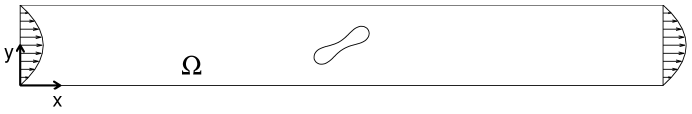
Figure 1: Schematic of a single red blood cell in plane Poiseuille flow with the computational domain $\Omega$.

An RBC with the viscosity of the cytoplasm same as that of the blood plasma is suspended in a fluid domain $\Omega$ filled with blood plasma which is incompressible and Newtonian as in Figure 1. For some $T>0$, the governing equations for the fluid-cell system are the Navier-Stokes equations

$$\rho_{f}\left(\dfrac{\partial{\bf u}}{\partial t}+{\bf u}\cdot\nabla{\bf u}\right)=-\nabla p+\mu\triangle{\bf u}+{\bf f},\text{ in }\Omega\times(0,T),$$ (1)

$$\nabla\cdot{\bf u}=0,\text{ in }\Omega\times(0,T).$$ (2)

Equations (1) and (2) are completed by the following boundary and initial conditions:

$${\bf u}={\bf 0}\text{ on the top and bottom of $\Omega$ and ${\bf u}$ is periodic in the $x$ direction,}$$ (3)

$${\bf u}({\bf x},0)={\bf u}_{0}({\bf x}),\text{ in }\Omega$$ (4)

where ${\bf u}$ and $p$ are the fluid velocity and pressure, respectively, $\rho_{f}$ is the fluid density, and $\mu$ is the fluid viscosity, which is assumed to be constant for the entire fluid. In eq. (1), ${\bf f}$ is a body force which is the sum of ${\bf f}_{p}$ and ${\bf f}_{B}$ where ${\bf f}_{p}$ is the pressure gradient pointing in the $x$ direction and ${\bf f}_{B}$ accounts for the force acting on the interface between fluid and cell. In eq. (4), ${\bf u}_{0}({\bf x})$ is the initial fluid velocity.

The deformability and the elasticity of the RBC are due to the skeleton architecture of the membrane. A two-dimensional elastic spring model used in [28] is considered in this paper to describe the deformable behavior of the RBCs. Based on this model, the RBC membrane can be viewed as membrane particles connecting with the neighboring membrane particles by springs, as shown in Figure 2. Energy stores in the spring due to the change of the length $l$ of the spring with respect to its reference length $l_{0}$ and the change in angle $\theta$ between two neighboring springs. The total energy of the RBC membrane, $E=E_{l}+E_{b}$, is the sum of the total energy for stretch and compression and the total energy for the bending which, in particular, are

$$E_{l}=\frac{k_{l}}{2}\sum_{i=1}^{N}(\frac{l_{i}-l_{0}}{l_{0}})^{2},\ \ E_{b}=\frac{k_{b}}{2}\sum_{i=1}^{N}\tan^{2}(\theta_{i}/2).$$ (5)

In equation (5), $N$ is the total number of the spring elements, and $k_{l}$ and $k_{b}$ are spring constants for changes in length and bending angle, respectively. The cell shape is stimulated by reducing the total area of the circle of radius $R_{0}=2.8\rm{\ \mu m}$ through a penalty function

$$\Gamma_{s}=\frac{k_{s}}{2}(\frac{s-s_{e}}{s_{e}})^{2}$$ (6)

where $s$ and $s_{e}$ are the time dependent area of the RBC and the specified area of the RBC, respectively, and the total energy is modified as $E+\Gamma_{s}$. Based on the principle of virtual work the force acting on the $i$th membrane particle now is

$${\bf F}_{i}=-\frac{\partial(E+\Gamma_{s})}{\partial{\bf r}_{i}}$$ (7)

where ${\bf r}_{i}$ is the position of the $i$th membrane particle. The value of the swelling ratio of an RBC in this paper is defined by $s^{*}=s_{e}/(\pi R_{0}^{2})$.

Figure 2: The elastic spring model of the RBC membrane.

The motion of the RBCs in the fluid flow is simulated by combining the immersed boundary method [29, 30, 31] and the aforementioned elastic spring model for RBC membrane. The Navier-Stokes equations for fluid flow have been solved by using an operator splitting technique and finite element method [32, 33] with a regular triangular mesh so that the specialized fast solver, such as FISHPAK by Adams et al. [34], can be used to solve the fluid flow. The methodologies have been validated in previous studies [18, 33].

2.2 Model and method for a neutrally buoyant particle

We suppose that $\Omega$ is filled with an incompressible viscous Newtonian fluid of the density $\rho_{f}$ and viscosity $\mu$. Let $B(t)$ be a freely moving rigid neutrally buoyant particle in a fluid as in Figure 3. The boundaries of $\Omega$ and $B(t)$ are denoted by $\Gamma$ and $\partial B$, respectively. For some $T>0,$ the governing equations for the fluid-particle system are the Navier-Stokes equations for the fluid flow:

Figure 3: Schematic of a neutrally buoyant particle in plane Poiseuille flow with the domain $\Omega$.

$$\rho_{f}(\dfrac{\partial{\bf u}}{\partial t}+({\bf u}\cdot{\boldsymbol{\nabla}}){\bf u})={\bf f}-{\boldsymbol{\nabla}}p+2\mu{\boldsymbol{\nabla}}\cdot{\bf D}({\bf u})\ \ in\ \Omega\backslash\overline{B(t)},\,t\in(0,T),$$ (8)

$$\nabla\cdot\textbf{u}=0\ \ in\ \Omega\backslash\overline{B(t)},\,t\in(0,T),$$ (9)

$${\bf u}({\bf x},0)={\bf u}_{0}({\bf x}),\ \ \forall{\bf x}\in\Omega\backslash\overline{B(0)},\ with\,\nabla\cdot{\bf u}_{0}=0,$$ (10)

$${\bf u}={\bf 0}\ \ on\ \Gamma,$$ (11)

$${\bf u}={{\bf V}}_{p}+\omega\times\stackrel{{\scriptstyle\longrightarrow}}{{{\bf G}{\bf x}}},\ \forall{\bf x}\in\partial B(t),\,$$ (12)

where ${\bf u}$ is the flow velocity, $p$ is the pressure, $2{\bf D}({\bf u})={\boldsymbol{\nabla}}{\bf u}+({\boldsymbol{\nabla}}{\bf u})^{t}$, and ${\bf f}$ is the pressure gradient pointing in the $x$ direction. In (12), the no-slip condition on the boundary of the particle, ${\bf V}_{p}$ is the translation velocity, $\omega\times\stackrel{{\scriptstyle\longrightarrow}}{{{\bf G}{\bf x}}}=(-\omega(y-G_{2}),\omega(x-G_{1}))^{t}$ where $\omega$ is the angular velocity, ${\bf G}=(G_{1},G_{2})^{t}$ is the mass center and ${\bf x}=(x,y)^{t}$ is a point on the boundary of the particle.

The motion of the particles is modeled by Newton’s laws:

$$M\ \dfrac{d{\bf V}_{p}}{dt}=M{\bf g}+{\bf F},\,I\dfrac{d\omega}{dt}={F}^{t},\,\dfrac{d{\bf G}}{dt}={\bf V}_{p},\,\dfrac{d\theta}{dt}=\omega,$$ (13)

$${\bf G}(0)={\bf G}^{0},{\bf V}_{p}(0)={\bf V}^{0}_{p},\omega(0)={\omega}^{0},\theta(0)=\theta^{0}.$$ (14)

In (13)-(14), ${\bf g}$ is the gravity, $\theta$ is the inclination angle between the long axis and the horizontal direction, $M$ and $I$ are the the mass and the moment of inertia of the particle, respectively; ${\bf F}$ and ${F}^{t}$ denote, respectively, the hydrodynamic force and the related torque imposed on the particle by the fluid given by

$${\bf F}=-\int_{\partial B}{\boldsymbol{\sigma}}{{\bf n}}\,ds,\ {F}^{t}=-\int_{\partial B}{{\bf G}{\bf x}}\times{\boldsymbol{\sigma}}{{\bf n}}\,ds,$$

where ${\boldsymbol{\sigma}}$ is the stress tensor, ${\bf x}$ is the generic point on the boundary of the particle, ${\bf n}$ is the unit normal vector on the boundary of the particle pointing to the center of the particle and ${\bf a}\times{\bf b}=a_{1}b_{2}-a_{2}b_{1}$ for the two dimensional cases.

The method of solution for the above fluid-particle interaction is a combination of a distributed Lagrange multiplier based fictitious domain method, the operator splitting methods and finite element methods (e.g., [27, 32, 35]). The basic idea is to imagine that the fluid fills the entire space inside as well as outside the particle boundaries. The fluid flow problem is then posed on a larger domain (the “fictitious domain”). This larger domain is simpler, allowing a simple regular mesh to be used, which in turn renders use of specialized fast solution techniques as in the previous section. The larger domain is also time independent, so the same mesh can be used for the entire simulation, eliminating the need for repeated remeshing and projection. The fluid inside the particle boundary must exhibit a rigid body motion. This constraint is enforced by using the distributed Lagrange multiplier, which represents the additional body force per unit volume needed to maintain the rigid body motion inside the particle boundary, much like the pressure in incompressible fluid flow, whose gradient is the force required to maintain the constraint of incompressibility. The computational method has been validated in our previous studies [35] and [27] for the motion of neutrally buoyant disks and elliptical cylinders, respectively, in Poiseuille flow. In this paper, we have applied the method to the cases of neutrally buoyant cylinder of a long body shape freely moving in bounded Poiseuille flows.

3 Simulation results and discussions

3.1 Oscillating motion of a single RBC in a narrower channel

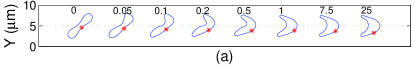
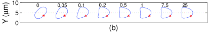
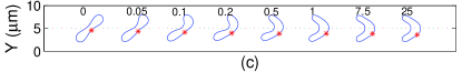
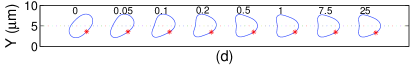
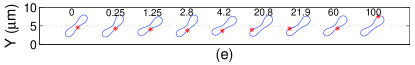
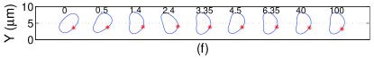
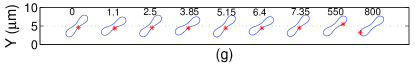
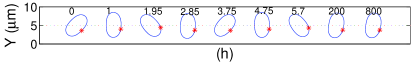
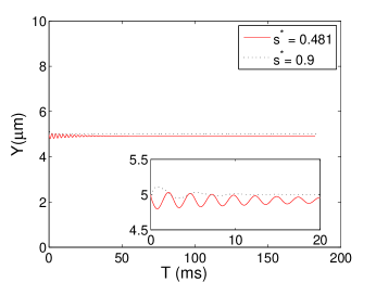
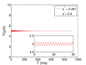
Figure 4: (Color online). The snapshots of the cell migration in Poiseuille flows for $s^{*}$=0.481 and 0.9 with different bending constants at different time ($\rm{ms}$): (a) $s^{*}$ = 0.481 and 0.1$k_{b}$, (b) $s^{*}$ = 0.9 and 0.1$k_{b}$, (c) $s^{*}$ = 0.481 and 1$k_{b}$, (d) $s^{*}$ = 0.9 and 1$k_{b}$, (e) $s^{*}$ = 0.481 and 10$k_{b}$, (f) $s^{*}$ = 0.9 and 10$k_{b}$, (g) $s^{*}$ = 0.481 and 100$k_{b}$, and (h) $s^{*}$ = 0.9 and 100$k_{b}$. The red asterisk denotes the same node point on the cell membrane. $R_{0}/w=$ 0.56. The initial position is (5,5) at the channel centerline and the initial inclination angle is $\pi/4$.

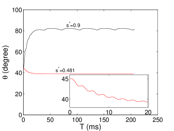
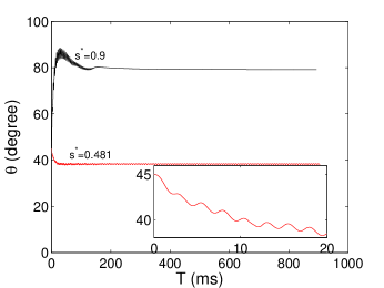
Figure 5: (Color online). The history of the position of the cell mass center in Poiseuille flows for s*=0.481 and 0.9 with different bending constants: 10$k_{b}$ (left) and 100$k_{b}$ (right). $R_{0}/w=$ 0.56. The initial position is (5,5) at the channel centerline and the initial inclination angle is $\pi/4$.

Figure 6: (Color online). The history of the inclination angle $\theta$ between the long axis of cell and the horizontal line for the bending constants 10$kb$ (left) and 100$kb$ (right). The initial position is (5,5) at the channel centerline and the initial inclination angle is $\pi/4$.

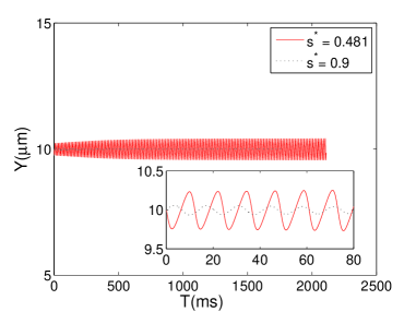
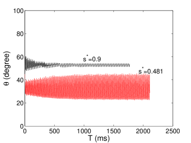
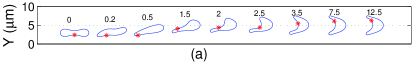
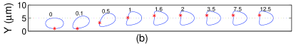
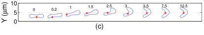
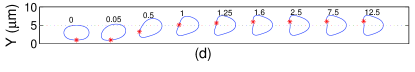
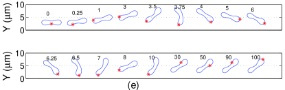
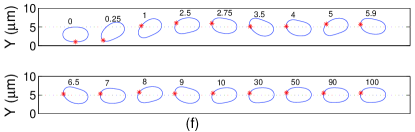
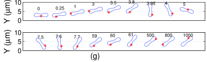
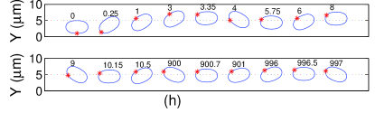
Figure 7: (Color online). The history of the position of the cell mass center (left) and inclination angle (right) for s*=0.481 and 0.9 with the bending constant 100$k_{b}$ in a channel of height 20 $\mu$m. The initial position is (5,10) at the channel centerline and the initial inclination angle is $\pi/4$.

Figure 8: (Color online). The snapshots of the cell migration in Poiseuille flows for $s^{*}$=0.481 and 0.9 with different bending constants at different time ($\rm{ms}$): (a) $s^{*}$ = 0.481 and 0.1$k_{b}$, (b) $s^{*}$ = 0.9 and 0.1$k_{b}$, (c) $s^{*}$ = 0.481 and 1$k_{b}$, (d) $s^{*}$ = 0.9 and 1$k_{b}$, (e) $s^{*}$ = 0.481 and 10$k_{b}$, (f) $s^{*}$ = 0.9 and 10$k_{b}$, (g) $s^{*}$ = 0.481 and 100$k_{b}$, and (h) $s^{*}$ = 0.9 and 100$k_{b}$. The red asterisk denotes the same node point on the cell membrane. The initial position is (5,3) and the initial inclination angle is 0.

Two motions of oscillation and vacillating-breathing (swing) of an RBC are observed in a narrow (100 $\times$ 10 $\rm{\mu m}^{2}$) channel considered here. The values of parameters for modeling cells are same with [18, 19] as follows: The bending constant is $k_{b}=5\times 10^{-10}$ $\rm{Nm}$, the spring constant is $k_{l}=5\times 10^{-8}$ $\rm{Nm}$, and the penalty coefficient is $k_{s}=10^{-5}$ $\rm{Nm}$. The swelling ratios of the cells in the simulations are $s^{*}$ = 0.481 and 0.9. The cells are suspended in blood plasma which has a density $\rho=1.00$ $\rm{g/cm^{3}}$ and a dynamical viscosity $\mu$ = 0.012 $\rm{g/(cms)}$. The viscosity ratio which describes the viscosity contrast of the inner and outer fluid of the RBC membrane is fixed at 1.0. The computational domain is a two dimensional horizontal channel. In addition, periodic conditions are imposed at the left and right boundary of the domain. The Reynolds number is defined by $Re={\rho}UH/\mu$, where $U$ is the average velocity in the channel, and $H$ is the height of the channel. To obtain a Poiseuille flow, a constant pressure gradient is prescribed as a body force so that the Reynolds number of the Poiseuille flow without cell is about 0.4167. We consider the motion of a single RBC with four different bending constants which are 0.1$k_{b}$, 1$k_{b}$, 10$k_{b}$, and 100$k_{b}$ in a Poiseuille flow with the fluid domain 100 $\times$ 10 $\rm{\mu m}^{2}$ (the degree of confinement $R_{0}/w$ = 0.56). The initial velocity is zero everywhere. The grid resolution for the computational domain is 64 grid points per 10 $\rm{\mu m}$.

First we have studied the cases in which the initial position of the cell mass center is located at the centerline and the initial inclination angle is $\theta=\pi/4$. Different motions led by the different bending constants are observed. When the bending constants are 0.1$k_{b}$ and 1$k_{b}$, the cells of both swelling ratios stay at the center region of the channel and the parachute shapes have been obtained for both cells as shown in Figures 6 $(a)$-$(d)$. For the bending constant 10$k_{b}$, the cell of swelling ratio $s^{*}$ = 0.481 exhibits a damped oscillation with deformation (called the vacillating-breathing behavior [4]) until it attains the equilibrium state aligning itself at an angle with the direction of the flow as shown in Figures 6 $(e)$ and 6. The cell has a slipper shape whose mass center is slightly away from the center line as studied in [19]. But the one of swelling ratio $s^{*}$ = 0.9 only has oscillating motion for shorter period of time (see Figure 6 $(f)$) and the cell gradually deforms into a parachute shape. When the bending constant is 100$k_{b}$, both cells first exhibit damped oscillation with the shapes of long body and, at the end, align themselves with a fixed inclination angle with respect to the flow direction as in Figures 6 $(g)$, $(h)$ and 6. The histories of the height of the cell mass center in Figure 6 do show the correlation with the oscillating motion. The initial inclination angle $\theta=\pi/4$ helps the fluid flow to create the oscillation of the cell mass center and then the flow field, which is about a full quadratic profile, interacting with the long body creates the oscillation similar to the one in [20]. But the cell mass center gradually approaches to an equilibrium height due to the interaction between the deformability of the cell and the Poiseuille flow and the wall effect as in Figure 6 and at the same time the oscillating motion is damping out accordingly as shown by the histories of the inclination angle in Figure 6. Once the oscillation of the cell mass center damps out, the inclination angle then is fixed as in Figures 6 and 6.

When increasing the channel height to 20 $\rm{\mu m}$ and keeping the other parameters same, we have focused now on the cases of the bending constant 100$k_{b}$. In Figure 8, the histories show that the oscillation of inclination angle become periodic. These cells with the bending constant 100$k_{b}$ stay at the channel central region since they are not neutrally buoyant rigid particle and and the deformability plus the Poiseuille flow profile keeps them staying in the channel central region. But the wall effect is weaker in a twice wider channel so that the up and down motion of the mass center does not damps out fast as in the channel of height 10 $\rm{\mu m}$.

When placing the initial position of the cell mass center off the centerline in a channel of height of 10 $\rm{\mu m}$ , we have obtained almost similar behaviors for both cells in Poiseuille flow as shown in Figures 8, 10 and 10. The vacillating-breathing behavior for the case of the bending constant 10$k_{b}$ and the oscillating motion for the case of the bending constant 100$k_{b}$ are stronger for the cell of $s^{*}=0.481$ since the lateral migration toward the channel central region enhances the oscillation. But another interesting result is the motion of the cell of $s^{*}=0.9$ for the bending constants 10$k_{b}$ and 100$k_{b}$ as shown in Figures 8 $(f)$ and $(h)$. A similar motion called snaking motion in Poiseuille flow has been studied in the Stokes regime in [37].

Concerning the oscillating motion and vacillating-breathing motion in Poiseuille flow, the bending constant needs to be large enough with respect to the maximum velocity of the fluid flow $u_{\textrm{max}}$ so that the cell can not be deformed into a symmetric parachute in the channel central region, but maintain a long body shape to interact with Poiseuille flow.

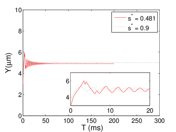
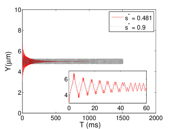
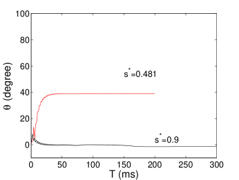
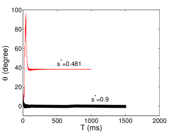
Figure 9: (Color online). The history of the position of the cell mass center in Poiseuille flows for s*=0.481 and 0.9 with different bending constants: 10$k_{b}$ (bottom left), and 100$k_{b}$ (bottom right). The initial position is (5,3) and the initial inclination angle is 0.

Figure 10: (Color online). The history of the angle between the long axis of cell and the horizontal line for the bending constants 10$kb$ (left) and 100$kb$ (right). The initial position is (5,3) and the initial inclination angle is 0.

3.2 Oscillating motion of a neutrally buoyant particle in a narrower channel

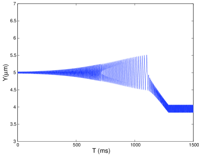
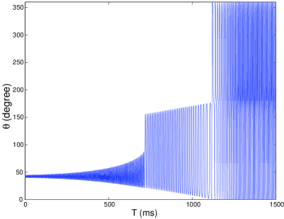
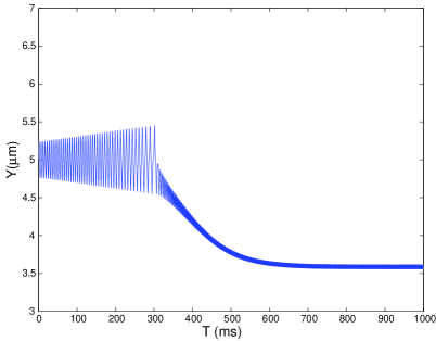
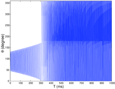
Figure 11: (Color online). History of particle mass center and inclination angle of the biconcave particle with $s^{*}=0.481$(top two) and the elliptic particle with $s^{*}=0.9$ (bottom two).

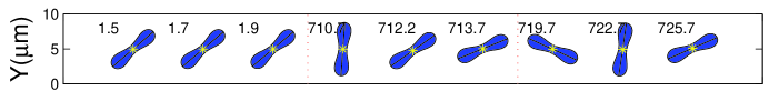
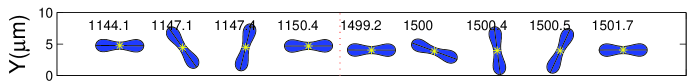
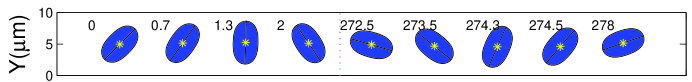
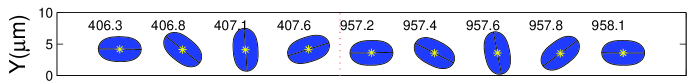
Figure 12: (Color online). Snapshots of particle motion in a narrow channel with the initial position of the mass center at the channel centerline. (i). Biconcave shape: $0^{o}<\theta<90^{o}$ for $1.5\leq t\leq 1.9$ and $710.7\leq t\leq 713.7$, $0^{o}<\theta<180^{o}$ for $719.7\leq t\leq 725.7$ and $1144.1\leq t\leq 1150.4$, and tumbling for $1499.2\leq t\leq 1501.7$. (ii) Elliptical shape: $0^{o}<\theta<180^{o}$ for $0\leq t\leq 2$ and $272.5\leq t\leq 278$ and tumbling $406.3\leq t\leq 407.6$ and $957.2\leq t\leq 958.1$. The number above each particle indicates the time (time unit is ms).

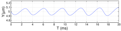
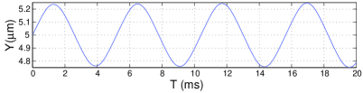
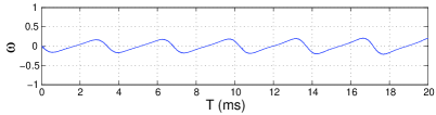
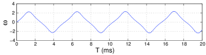
Figure 13: (Color online). The histories of particle mass position (top) and the angular velocity (bottom) with $s^{*}=0.481$ (left two) and $s^{*}=0.9$ (right two) for $0\leq t\leq 20$.

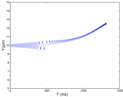
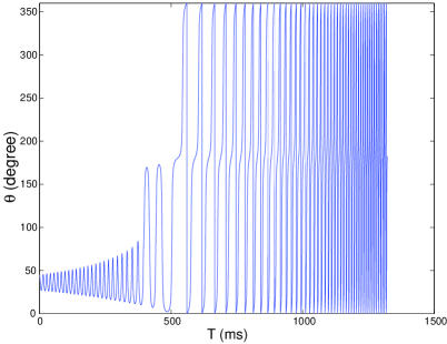
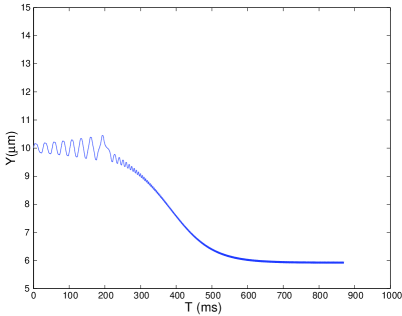
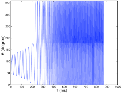
Figure 14: (Color online). History of particle mass center and inclination angle of the biconcave particle with $s^{*}=0.481$(top two) and the elliptic particle with $s^{*}=0.9$ (bottom two) in a channel of height 20 $\rm{\mu m}$.

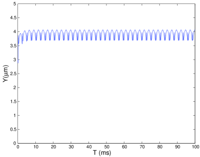
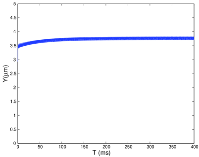
Figure 15: (Color online). History of particle mass center of the biconcave particle with $s^{*}=0.481$ (left) and the elliptic particle with $s^{*}=0.9$ (right). The initial mass center is off the centerline.

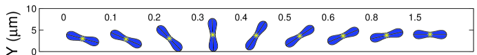
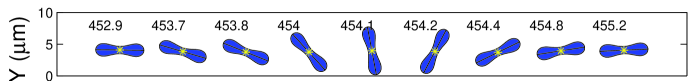
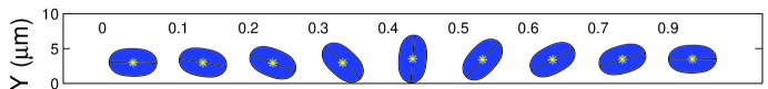
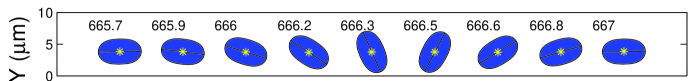
Figure 16: (Color online). Snapshots of particle motion in narrow channel with the initial position of the mass center away from the channel centerline. The number above each snapshot denotes when the snapshot was taken(time unit is ms).

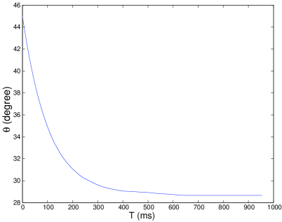
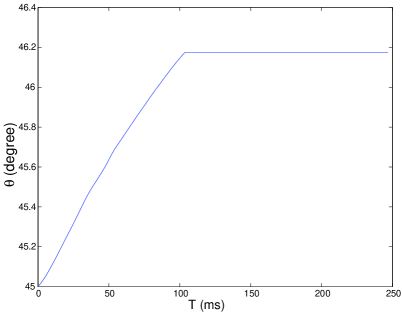
Figure 17: (Color online). History of particle inclination angle when forced to stay at channel center with $s^{*}=0.481$ (left) and $s^{*}=0.9$ (right)

The motion of a neutrally buoyant particle of either biconcave or elliptical shape in a narrow channel (100 $\times$ 10 $\rm{\mu m}^{2}$) has been studied in this section. The biconcave and elliptical shapes are obtained based on the cell resting shapes used in the previous section. The long axis of the biconcave shape (resp., elliptical shape) is 7.65 $\rm{\mu m}$ (resp., 6.825$\rm{\mu m}$). The particle is suspended in an incompressible Newtonian fluid of the density $\rho=1.00$ $\rm{g/cm^{3}}$ and the dynamical viscosity $\mu$ = 0.012 $\rm{g/(cms)}$. A constant pressure gradient is chosen as in the previous section so that the $Re$ of the flow without particle is about 0.4167.

We have first considered the motions of the particle mass center of both shapes initially located at the centerline of the channel with the initial inclination angle $\theta=\pi/4$. As in Figures 11 and 12, both particles show an oscillating motion of the mass center about the channel center. The up and down motion together with the Poiseuille flow velocity profile cause the particles to oscillate in the inclination angle. As the up and down motion becomes stronger, the oscillation in inclination angle keeps increasing its range. For the particle of biconcave shape, the oscillation of inclination angle is first between 0 and 90 degrees and then the particle starts to swing back and forth with the inclination angle oscillating between 0 and 180 degrees. Once the particle turns horizontal, it starts a tumbling motion and ends the oscillation of the inclination angle. The mass center of the tumbling particle migrates toward an equilibrium position between the channel centerline and the wall. The initial inclination angle $\theta=\pi/4$ helps the fluid flow to create the oscillation of the particle mass center as shown in Figure 13. At the beginning once the mass center is pushing down by the Poiseuille flow, the inclination angle is decreasing since the upper portion of the particle close to the centerline moves forward faster than the lower portion away from the centerline does. The wall effect from the bottom wall slows down the lateral migration and finally push the neutrally buoyant particle away. When it crosses the centerline, the angular velocity changes sign accordingly as in Figure 13. The neutrally buoyant particle goes through the same up and down motion with rotation changing its direction accordingly which is similar to the one in the Stokes regime in [20]. But the neutrally buoyant particle moves up and down about the centerline with increasing amplitude and finally breaks away from the centerline and moves to its equilibrium position between the centerline and the wall as shown in Figure 11. The elliptic shape particle has a similar motion, but the oscillation of the inclination angle is always a back and forth swing motion before the tumbling motion occurs. This difference in motion is due to the shape difference of the particles. The particle of biconcave shape undertakes stronger resistance force from the flow while the flow can smoothly bypass the particle of elliptic shape. This also explains why it takes the particle of biconcave shape longer time to turn to a tumbling motion than the particle of elliptic shape does.

When increasing the channel height to 20 $\rm{\mu m}$ and keeping the other parameters same, both the up and down motion of the mass center and the rotation of the long body oscillates stronger since the wall effect is weaker in a twice wider channel. The neutrally buoyant particle of long body shape behaves similarly but they migrate away from the centerline faster than they do in the channel of height 10 $\rm{\mu m}$.

When the initial mass center is off the centerline, the particle directly turns into a tumbling motion and migrates toward the equilibrium position between the channel centerline and the wall in Figure 15. When the particle reaches its equilibrium position, it shows a rotation with periodically varying angular velocity as in [27]. The neutrally buoyant particle behavior is entirely different from the cell motion discussed in the previous section due to the lack of the deformability. In Figure 16, two plots of snapshots of the tumbling motion are shown for each swelling ratio. The first plot is for the first tumbling motion of the particle where as the second plot is the snapshot of one tumbling motion when the particle has reached its equilibrium position. By comparing the time in the first and second plots, one can observe that it takes longer time for the particle to spin a whole circle at the equilibrium position than in the first few spins. This is because under the parabolic velocity profile, the flow shear rate is higher when the particle is further away from the channel center. So the angular velocity is larger in the first few spins since the position of the particle is closer to the channel wall.

To further study the effect of the up and down motion about the centerline of the mass center, we have added a constraint on the particle motion so that the particle is only allowed to move freely in the horizontal direction and rotate freely. In Figure 17, the inclination angle of the constrained motion of a neutrally buoyant particle reaches to an equilibrium angle without any oscillation when moving along the centerline in the channel. It shows that the up and down motion of the mass center in the central region of the Poiseuille flow causes the oscillation of the inclination angle.

4 Conclusion

We have compared the oscillating motions of a neutrally buoyant particle and a red blood cell in Poiseuille flow in a narrow channel to understand the oscillating motions in [18, 19] and to find out the difference between the cell motion and the particle motion. For the motion of a neutrally buoyant particle of either biconcave or elliptical shape, we have obtained oscillating motion in Poiseuille flow when the particle mass center is placed at the centerline initially. But the neutrally buoyant particle moves up and down about the centerline with the amplitude which is increasing in time and finally breaks away from the centerline and moves to its equilibrium position between the centerline and the wall. The neutrally buoyant particle behavior is entirely different from the cell motion due to the lack of the deformability. Concerning the cell motion in the central region of the channel, the oscillating motion occurs exactly like a long rigid body as long as the cell mass center moves up and down in the channel central region and the cell can maintain a long body shape. But when the mass center of the neutrally buoyant particle of a long body shape is not allowed to move up and down, its inclination angle reaches a fixed angle without any oscillation. Thus the up-and-down motion of the mass center in the channel central region triggers the oscillation motion of a long body entity in Poiseuille flows.

References

- [1] K. H. de Haas, C. Blom, D. van den Ende, M. H. G. Duits, and J. Mellema, “Deformation of giant lipid bilayer vesicles in shear flow,” Phys. Rev. E. 56, 7132 (1997).
- [2] V. Kantsler and V. Steinberg, “Transition to tumbling and two regimes of tumbling motion of a vesicle in shear flow,” Phys. Rev. Lett. 96, 036001 (2006); “Orientation and dynamics of a vesicle in tank-treading motion in shear flow,” Phys. Rev. Lett. 95, 258101 (2005).
- [3] U. Seifert, “Fluid membranes in hydrodynamic flow fields: Formalism and an application to fluctuating quasispherical vesicles in shear flow,” Eur. Phys. J. B. 8, 405 (1999).
- [4] C. Misbah, “Vacillating Breathing and Tumbling of Vesicles under Shear Flow,” Phys. Rev. Lett. 96, 028104 (2006).
- [5] M. Kraus, W. Wintz, U. Seifert, and R. Lipowsky, “Fluid Vesicles in Shear Flow,” Phys. Rev. Lett. 77, 3685 (1996).
- [6] J. Beaucourt, F. Rioual, T. Seń, T. Biben, and C. Misbah, “Steady to unsteady dynamics of a vesicle in a flow,” Phys. Rev. E. 69, 011906 (2004).
- [7] H. Noguchi and G. Gompper, “Fluid vesicles with viscous membranes in shear flow,” Phys. Rev. Lett. 93, 258102 (2004).
- [8] H. Noguchi and G. Gompper, “Dynamics of fluid vesicles in shear flow: Effect of membrane viscosity and thermal fluctuation,” Phys. Rev. E. 72, 011901 (2005).
- [9] H. Noguchi and G. Gompper, “Swinging and tumbling of fluid vesicles in shear flow,” Phys. Rev. Lett. 98, 128103 (2007).
- [10] G. Danker and C. Misbah, “Rheology of a dilute suspension of vesicles,” Phys. Rev. Lett. 98, 088104 (2007).
- [11] Y. Kim and M.-C. Lai, “Numerical study of viscosity and inertial effects on tank-treading and tumbling motions of vesicles under shear flow,” Phys. Rev. E. 86, 066321 (2012).
- [12] T. M. Fischer, M. Stöhr-Liesen, and H. Schmid-Schönbein, “The red cell as a fluid droplet: tank tread-like motion of the human erythrocyte membrane in shear flow,” Science. 202, 894 (1978).
- [13] S. R. Keller and R. Skalak, “Motion of a tank-treading ellipsoidal particle in a shear flow,” J. Fluid Mech. 120, 27 (1982).
- [14] R. Tran-Son-Tay, S. P. Sutera, and P. R. Rao, “Determination of red blood cell membrane viscosity from rheoscopic observations of tank-treading motion,” Biophys. J. 46, 65 (1984).
- [15] C. Pozrikidis, “Numerical Simulation of the Flow-Induced Deformation of Red Blood Cells,” Ann. Biomed. Eng. 31, 1194 (2003).
- [16] J. M. Skotheim and T. W. Secomb, “Red blood cells and other nonspherical capsules in shear flow: oscillatory dynamics and the tank-treading-to-tumbling transition,” Phys. Rev. Lett. 98, 078301 (2007).
- [17] M. Abkarian, M. Faivre, and A. Viallat, “Swinging of red blood cells under shear flow,” Phys. Rev. Lett. 98, 188302 (2007).
- [18] L. Shi, T.-W. Pan, and R. Glowinski, “Deformation of a single blood cell in bounded Poiseuille flows,” Phys. Rev. E. 85, 016307 (2012).
- [19] L. Shi, T.-W. Pan, and R. Glowinski, “Lateral migration and equilibrium shape and position of a single red blood cell in bounded Poiseuille flows,” Phys. Rev. E 86, 056308 (2012).
- [20] M. Sugihara-Seki, “The motion of an elliptical cylinder in channel flow at low Reynolds numbers,” J. Fluid Mech. 257, 575 (1993).
- [21] G. Segre and A. Silberberg, “Radial particle displacements in Poiseuille flow of suspensions,” Nature. 189, 209 (1961).
- [22] G. Segre and A. Silberberg, “Behavior of macroscopic rigid spheres in Poiseuille flow,” J. Fluid. Mech. 14, 136 (1962).
- [23] E. S. Asmolov, “The inertial lift on a spherical particle in a plane Poiseuille flow at large channel Reynolds number,” J. Fluid Mech. 381, 63 (1999).
- [24] E. S. Asmolov, “The inertial lift on a small particle in a weak-shear parabolic flow,” Phys. Fluids. 14, 15 (2002).
- [25] S. Eloot1, F. De Bisschop, and P. Verdonck, “Experimental evaluation of the migration of spherical particles in three-dimensional Poiseuille flow,” Phys. Fluids. 16, 2282 (2004).
- [26] B. H. Yang, J. Wang, D. D. Joseph, H. H. Hu, T.-W. Pan, and R. Glowinski, “Numerical study of particle migration in tube and plane Poiseuille flows,” J. Fluid Mech. 540, 109 (2005).
- [27] S.-D. Chen, T.-W. Pan, and C.-C. Chang, “The Motion of a Single and Multiple Neutrally Buoyant Elliptical Cylinders in Plane Poiseuille Flow,” Phys. Fluids. 24, 103302 (2012).
- [28] K. Tsubota, S. Wada, and T. Yamaguchi, “Simulation Study on Effects of Hematocrit on Blood Flow Properties Using Particle Method,” J. Biomech. Sci. Eng. 1, 159 (2006).
- [29] C. S. Peskin, “Numerical analysis of blood flow in the heart,” J. Comput. Phys. 25, 220 (1977).
- [30] C. S. Peskin and D. M. McQueen, “Modeling prosthetic heart valves for numerical analysis of blood flow in the heart,” J. Comput. Phys. 37, 11332 (1980).
- [31] C. S. Peskin, “The immersed boundary method,” Acta Numer. 11, 479 (2002).
- [32] R. Glowinski, “Finite element methods for incompressible viscous flow,” in Handbook of Numerical Analysis, Vol. IX, P. G. Ciarlet and J. L. Lions (Eds.), North-Holland: Amsterdam, 7 (2003).
- [33] L. Shi, T.-W. Pan, and R. Glowinski, “Numerical simulation of lateral migration of red blood cells in Poiseuille flows,” Int. J. Numer. Methods Fluids. 68, 1393 (2012).
- [34] J. Adams, P. Swarztrauber, and R. Sweet, “FISHPAK: A package of Fortran subprograms for the solution of separable elliptic partial differential equations, The National Center for Atmospheric Research,” Boulder, CO, 1980.
- [35] T.-W. Pan and R. Glowinski, “Direct simulation of the motion of neutrally buoyant circular cylinders in plane Poiseuille flow,” J. Comp. Phys. 181, 260 (2002).
- [36] T.-W. Pan, L. Shi, and R. Glowinski, “A DLM/FD/IB method for simulating cell/cell and cell/particle interaction in microchannels,” Chinese Ann. Maths. B. 31, 975 (2010).
- [37] B. Kaoui1, N. Tahiri, T. Biben, H. Ez-Zahraouy, A. Benyoussef, G. Biros, and C. Misbah, “Complexity of vesicle microcirculation,” Phys. Rev. E. 84, 041906 (2011).