Non Total-Unimodularity Neutralized Simplicial Complexes

Abstract

Given a simplicial complex $K$ with weights on its simplices and a chain on it, the Optimal Homologous Chain Problem (OHCP) is to find a chain with minimal weight that is homologous (over ${\mathbb{Z}}$) to the given chain. The OHCP is NP-complete, but if the boundary matrix of $K$ is totally unimodular (TU), it becomes solvable in polynomial time when modeled as a linear program (LP). We define a condition on the simplicial complex called non total-unimodularity neutralized, or NTU neutralized, which ensures that even when the boundary matrix is not TU, the OHCP LP must contain an integral optimal vertex for every input chain. This condition is a property of $K$, and is independent of the input chain and the weights on the simplices. This condition is strictly weaker than the boundary matrix being TU. More interestingly, the polytope of the OHCP LP may not be integral under this condition. Still, an integral optimal vertex exists for every right-hand side, i.e., for every input chain. Hence a much larger class of OHCP instances can be solved in polynomial time than previously considered possible. As a special case, we show that $2$-complexes with trivial first homology group are guaranteed to be NTU neutralized.

1 Introduction

Topological cycles in shapes capture their important features, and are employed in many applications from science and engineering. A problem of particular interest in this context is the optimal homologous cycle problem, OHCP, where given a cycle in the shape, the goal is to compute the shortest cycle in its topological class (homologous). For instance, one could generate a set of cycles from a simplicial complex using the persistence algorithm [16] and then tighten them while staying in their respective homology classes. The OHCP and related problems have been widely studied in recent years both for two dimensional complexes [2, 3, 5, 17, 12] and for higher dimensional instances [10, 23]. The OHCP with homology defined over the popularly used field of ${\mathbb{Z}}_{2}$ was known to be NP-hard [4]. But it was shown recently that if the homology is defined over ${\mathbb{Z}}$, then one could solve OHCP in polynomial time when the simplicial complex has no relative torsion [11]. The generalized decision version of the problem considering chains instead of cycles (also termed OHCP) was recently shown to be NP-complete [15]. Instances that fall in between these two extreme cases have not been studied so far. In particular, the complexity of OHCP in the presence of relative torsion is not known.

The polynomial time solvability of OHCP was shown by modeling the problem as a linear program (LP), and showing that the constraint matrix of this LP is totally unimodular (TU) when the simplicial complex does not have any relative torsion [11]. This connection between TU matrices and polynomial time solvability of integer programs (IPs) by solving their associated LPs is well known, e.g., see [21, Chap. 19–21]. If the constraint matrix of an LP is TU, then its polyhedron is integral, i.e., all its vertices have integral coordinates. Two other concepts associated with integral polyhedra that are weaker than TU matrices are $k$-balanced matrices [6, 7] and totally dual integral (TDI) systems [21, Chap. 22] [13]. But applications of such weaker conditions to the OHCP LP and their potential correspondences to the topology of simplicial complexes have not been explored so far.

Our Contributions:

We define a characterization of the simplicial complex termed non total-unimodularity neutralized, or NTU neutralized for short, which guarantees that even when there is relative torsion in the simplicial complex, every instance of the OHCP LP has an integer optimal solution. Under this condition, the OHCP instance for any input chain with homology defined over ${\mathbb{Z}}$ could be solved in polynomial time using linear programming even when the constraint matrix of the OHCP LP is not TU. We arrive at our main result by studying the structure of the OHCP LP, and characterizing several properties of its basic solutions. Recall that the vertices of an LP correspond to its basic feasible solutions. In particular, we prove that an OHCP LP for a given input chain has a fractional basic solution if and only if the OHCP LP with a component elementary chain, i.e., a chain with a single nonzero coefficient of $1$, as input has a certain fractional basic solution. Using this result, we show that no OHCP LP over the given simplicial complex has a unique fractional optimal solution if and only if every elementary chain involved in each relative torsion has a neutralizing chain in the complex, i.e., when the simplicial complex is NTU neutralized.

Our result partly fills the gap between the extreme cases of the OHCP LP solving the OHCP when the complex has no relative torsion, and the OHCP being NP-complete (there could well be instances that are amenable to efficient solutions by methods distinct from solving LPs). The condition of a complex being NTU neutralized is strictly weaker than requiring its boundary matrix to be TU, or even to be balanced. Further, this condition is a property of the simplicial complex, and is independent of the input chain as well as the choice of weights on the simplices. Hence a much broader class of OHCP instances can be solved in polynomial time using linear programming than previously considered possible. When the simplicial complex is NTU neutralized, the linear system in the dual of the OHCP LP is TDI. But this case does not appear to be covered by any of the currently known characterizations of TDI systems. In particular, the polytope of the OHCP LP may not be integral even when the complex is NTU neutralized. Still, an integral optimal solution exists for every integral right-hand side, i.e., for every input chain. As a special case, we show that every $2$-complex with trivial first homology group is guaranteed to be NTU neutralized.

1.1 An example, and some intuition

We illustrate the condition of a simplicial complex being NTU neutralized by describing a set of two dimensional complexes related to the Möbius strip. A $2$-complex having no relative torsion is equivalent to it having no Möbius strip [11, Thm. 5.13]. Consider the three different triangulations of a space in Figure 1. In the left and right complexes, we have a Möbius strip self-intersecting at one ($d$) and two vertices ($a,d$), respectively, resulting in relative torsion in both cases. In the middle complex, the self intersection is along the edge $ad$, hence we do not have relative torsion. Hence the boundary matrix is TU only for the middle complex. Still, in the right complex, the OHCP LP has an integral optimal solution for every input chain.

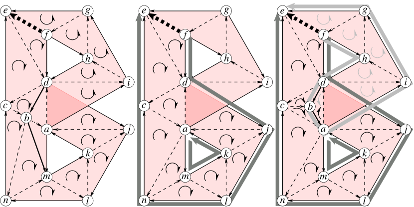
Figure 1: Three triangulations of a space. The right complex is NTU neutralized, the left one is not. The middle complex has a TU boundary matrix.

For example, consider the edge $ef$ (shown in thick dashes) with multiplier $1$ as the input chain. Let the edge weights be as follows: dashed and dotted edges have weight $1$, thin solid edges have weights of $0.05$, and thick solid edges have weights of $0.10$ each. The dashed edges are the “manifold” edges in the potential Möbius strip in each complex. The thin solid edges are boundary edges. The two pairs of thick solid edges are boundary edges in the candidate Möbius strips, but are each shared by two triangles in the simplicial complex. Solving the OHCP involves pushing the heavy manifold edge(s) onto the light boundary edges using the boundaries of triangles. In the left complex, the unique optimal solution to the OHCP LP corresponds to all the black solid edges, which is the boundary of the Möbius strip self-intersecting at vertex $d$, with coefficients $\pm 0.5$. This instance illustrates the case of minimal violation of TU we study in a general simplicial complex.

The optimal homologous chain is indicated in dark gray in the middle and right complexes (it is the same in all three complexes). In the right complex, there are two integral optimal solutions to the OHCP LP, which are outlined in dark and light gray. Any convex combination of these two chains also corresponds to an optimal solution of the OHCP LP, including the one made of all solid edges with coefficients $\pm 0.5$. This observation may be explained by the presence of a disk whose boundary is an odd number of dashed edges, e.g., triangle $adc$, which neutralizes the Möbius strip. This “odd disk” provides an alternative to pushing the heavy manifold edge onto all the light boundary edges by going around the entire Möbius strip with fractional multipliers. Instead, one could take a “shortcut” across the middle of the strip through the neutralizing chain, permitting integer multipliers. In this case, there also exists a complementary shortcut. The fractional solution going all the way around the strip is a convex combination of the two shortcut integral solutions. Our characterization of NTU neutralization generalizes this observation to arbitrary dimensions. Intuitively, a complex is NTU neutralized if there exists an “odd disk” providing such a shortcut across every relative torsion, for each of its “manifold” elementary chains (similar to edge $ef$ above).

Adding triangle $akm$ to the left complex makes it NTU neutralized. For instance, $adcbnmlkja$ is a disc whose boundary is $9$ dashed edges. Alternatively, adding both triangles $akm$ and $dfh$ to the left complex also makes it NTU neutralized. In this case, the first homology group becomes trivial, which is a sufficient condition for $2$-complexes to be NTU neutralized (Theorem 8.1).

2 Background

We recall some relevant basic concepts and definitions from algebraic topology and optimization. Refer to standard books, e.g., ones by Munkres [19] and by Schrijver [21], for details.

Given a vertex set $V$, a simplicial complex $K=K(V)$ is a collection of subsets $\{\sigma\subseteq V\}$ where $\sigma^{\prime}\subseteq\sigma$ is in $K$ if $\sigma\in K$. A subset $\sigma\in K$ of cardinality $q=p+1$ is called a $p$-simplex. If $\sigma^{\prime}\subseteq\sigma$ ($\sigma^{\prime}\subset\sigma$), we call $\sigma^{\prime}$ a face (proper face) of $\sigma$, and $\sigma$ a coface (proper coface) of $\sigma^{\prime}$. An oriented simplex $\sigma=\{v_{0},v_{1},\cdots,v_{p}\}$ or $v_{0}v_{1}\cdots v_{p}$ is an ordered set of vertices. The simplices $\sigma_{i}$ with coefficients $\alpha_{i}$ in ${\mathbb{Z}}$ can be added formally creating a chain $c=\Sigma_{i}\alpha_{i}\sigma_{i}$. These chains form the chain group ${\sf C}_{p}$. The boundary $\partial_{p}\sigma$ of a $p$-simplex $\sigma$, $p\geq 0$, is the $(p-1)$-chain that adds all the $(p-1)$-faces of $\sigma$ considering their orientations. This defines a boundary homomorphism $\partial_{p}:{\sf C}_{p}\rightarrow{\sf C}_{p-1}$. The kernel of $\partial_{p}$ forms the $p$-cycle group ${\sf Z}_{p}(K)$ and its image forms the $(p-1)$-boundary group ${\sf B}_{p-1}(K)$. The homology group ${\sf H}_{p}(K)$ is the quotient group ${\sf Z}_{p}(K)/{\sf B}_{p}(K)$. Intuitively, a $p$-cycle is a collection of oriented $p$-simplices whose boundary is zero. It is a nontrivial cycle in ${\sf H}_{p}$, if it is not a boundary of a $q$-chain.

For a finite simplicial complex $K$, the groups of chains ${\sf C}_{p}(K)$, cycles ${\sf Z}_{p}(K)$, and ${\sf H}_{p}(K)$ are all finitely generated abelian groups. By the fundamental theorem of finitely generated abelian groups [19, page 24] any such group $G$ can be written as a direct sum of two groups $G=F\oplus T$ where $F\cong({\mathbb{Z}}\oplus\cdots\oplus{\mathbb{Z}})$ and $T\cong({\mathbb{Z}}/t_{1}\oplus\cdots\oplus{\mathbb{Z}}/t_{k})$ with $t_{i}>1$ and $t_{i}$ dividing $t_{i+1}$. The subgroup $T$ is called the torsion of $G$. If $T=0$, we say $G$ is torsion-free.

For a subcomplex $L_{0}$ of a simplicial complex $L$, the quotient group ${\sf C}_{p}(L)/{\sf C}_{p}(L_{0})$ is called the group of relative $p$-chains of $L$ modulo $L_{0}$, denoted ${\sf C}_{p}(L,L_{0})$. The boundary operator $\operatorname{\partial}_{p}\colon{\sf C}_{p}(L)\rightarrow{\sf C}_{p-1}(L)$ and its restriction to $L_{0}$ induce a homomorphism

$$\operatorname{\operatorname{\partial}}_{p}^{\,(L,L_{0})}\colon{\sf C}_{p}(L,L_{0})\rightarrow{\sf C}_{p-1}(L,L_{0})\,.$$

Writing ${\sf Z}_{p}(L,L_{0})={\rm ker}\operatorname{\operatorname{\partial}}_{p}^{\,(L,L_{0})}$ for relative cycles and ${\sf B}_{p-1}(L,L_{0})=\operatorname{{\mathrm{i}m\,}}\operatorname{\operatorname{\partial}}_{p}^{\,(L,L_{0})}$ for relative boundaries, we obtain the relative homology group

$${\sf H}_{p}(L,L_{0})={\sf Z}_{p}(L,L_{0})/{\sf B}_{p}(L,L_{0}).$$

Given the oriented simplicial complex $K$ of dimension $d$, and a natural number $p$, $1\leq p\leq d$, the $p$-boundary matrix of $K$, denoted $[\partial_{p}]$, is a matrix containing exactly one column $j$ for each $p$-simplex $\sigma$ in $K$, and exactly one row $i$ for each $(p-1)$-simplex $\tau$ in $K$. If $\tau$ is not a face of $\sigma$, then the entry in row $i$ and column $j$ is 0. If $\tau$ is a face of $\sigma$, then this entry is $1$ if the orientation of $\tau$ agrees with the orientation induced by $\sigma$ on $\tau$, and $-1$ otherwise.

A matrix $A$ is totally unimodular (TU) if the determinant of each of its square submatrix is either $0,1$, or $-1$. Hence each $A_{ij}\in\{0,\pm 1\}$ as well. The importance of TU matrices for integer programming is well known [21, Chapters 19-21]. In particular, it is known that the integer linear program

$$\min\,\{\mathbf{f}^{T}\mathbf{x}~{}|~{}A\mathbf{x}=\mathbf{b},\;\mathbf{x}\geq\mathbf{0},\mathbf{x}\in{\mathbb{Z}}^{n}\}$$ (1)

for $A\in{\mathbb{Z}}^{m\times n},\mathbf{b}\in{\mathbb{Z}}^{n}$ can always, i.e., for every $\mathbf{f}\in{\mathbb{R}}^{n}$, be solved in polynomial time by solving its linear programming relaxation (obtained by ignoring $\mathbf{x}\in{\mathbb{Z}}^{n}$) if and only if $A$ is totally unimodular. This result was employed to show that the OHCP for the input $p$-chain $\mathbf{c}$ modeled as the following LP could be solved to get integer solutions under certain conditions [11, Eqn. (4)].

$$\min\; \sum_{i}\,\lvert w_{i}\rvert\,(x_{i}^{+}+x_{i}^{-})$$

subject to $$\mathbf{x}^{+}-\mathbf{x}^{-}=\mathbf{c}+[\operatorname{\partial}_{q}]\;\mathbf{y}$$ (2)

$$\mathbf{x}^{+},\;\mathbf{x}^{-}\geq\mathbf{0}\,.$$

We assume the weights $w_{i}$ for $p$-simplices are nonnegative. Replacing $\mathbf{y}$ with two nonnegative variable vectors $\mathbf{y}^{+}$ and $\mathbf{y}^{-}$, we rewrite the above LP in the following form.

$$\min~{} \begin{bmatrix}\mathbf{w}^{T}&\mathbf{w}^{T}&\mathbf{0}^{T}&\mathbf{0}^{T}\end{bmatrix}\mathbf{z}$$

subject to $$\begin{bmatrix}~{}I&\,-I&\,-B&~{}B~{}\end{bmatrix}\mathbf{z}=\mathbf{c}$$ (3)

$$\mbox{\hskip 100.81696pt}\mathbf{z}\geq\mathbf{0}.$$

Notice that $B=[\partial_{q}]$, and the variable vector $\displaystyle\mathbf{z}^{T}=\begin{bmatrix}\mathbf{x}^{+T}&\mathbf{x}^{-T}&\mathbf{y}^{+T}&\mathbf{y}^{-T}\end{bmatrix}$. Recall that $x^{+}_{i}$ and $x^{-}_{i}$ correspond to the $i{\text{th}}$ $p$-simplex, while $y^{+}_{j},y^{-}_{j}$ capture the coefficients for the $j{\text{th}}$ $q$-simplex. We refer to this formulation as the OHCP LP from now on. We let $P$ denote its feasible region, and let $A=\begin{bmatrix}I&-I&-B&B\end{bmatrix}$ be the constraint matrix of (3). It was shown that $A$ is TU, or equivalently, $P$ is integral if and only if $B$ is TU, which happens [11, Thm. 5.2] if and only if ${\sf H}_{p}\left(L,L_{0}\right)$ is torsion-free, for all pure subcomplexes $L_{0}$, $L$ in $K$ of dimensions $p$ and $q$ respectively, where $L_{0}\subset L$. Thus OHCP can be solved in polynomial time if the simplicial complex is free of relative torsion.

The point $\mathbf{z}$ is a vertex of $P$ if it is in $P$, but is not a convex combination of any two distinct elements of $P$ [21, Chap. 8]. A basic solution of a system of linear equations is a point in a solution space of dimension $d$ where a set of $d$ linearly independent constraints are active, i.e., satisfied as equations. If a basic solution of $P$ is feasible, then it is a vertex [21, Chap. 8].

3 Characterizations of Basic Solutions of the OHCP LP

Our goal is to characterize the fractional basic feasible solutions, or vertices, of the OHCP LP. Instead, we establish several properties of basic solutions, by relaxing feasibility. This step simplifies the analysis, and we prove that the basic solutions and vertices are equivalent in a certain sense as explained below (see Corollary 3.13).

Notice that $P$ is the hyperplane defined by the equality constraints, with the only bounds being the nonnegativity constraints. We use $P_{A}$ to denote the hyperplane that is $P$ without the bounds. We use $\mathbf{z}$ to refer to a general element of ${\mathbb{R}}^{2(m+n)}$, and call $z_{i}$ an $x$-entry if $i\leq 2m$, and a $y$-entry if $i>2m$.

Definition 3.1.

For any entry $z_{i}$ of $\mathbf{z}\in{\mathbb{R}}^{2(m+n)}$, its opposite entry is $z_{i+m}$ for $i\leq m,z_{i-m}$ for $m<i\leq 2m,z_{i+n}$ for $2m<i\leq 2m+n$, and $z_{i-n}$ for $2m+n<i\leq 2(m+n)$. We denote the opposite entry of $z_{i}$ as $z_{-i}$. Any pair of opposite entries are coefficients for the same simplex. Hence for a pair of opposite entries $z_{i},z_{-i}$ of $\mathbf{z}$, if at least one of the two is 0, then $\mathbf{z}$ is concise in the $i{\text{th}}$ entry. $\mathbf{z}$ is concise if it is concise in each entry.

The following definition translates coordinates of an OHCP LP solution to the $i{\text{th}}$ row or $j{\text{th}}$ column of $[\partial_{q}]$, and the $p$- and $q$-simplices the row and column represent, respectively.

Definition 3.2.

For a solution $\mathbf{z}$ of an OHCP LP, for any $i\leq m$, the $i{\text{th}}\ p$ coefficient is $z_{i}-z_{-i}$, and for any $j:2m<j\leq 2m+n$, the $(j-2m){\text{th}}\ q$ coefficient is $z_{j}-z_{-j}$.

In figures of simplices representing solutions to OHCP LPs, we generally show the $p$- and $q$-coefficients of simplices, and assume that all solutions illustrated are concise. When we call a set of solutions equivalent we mean each has the same $p$- and $q$-coefficients.

For any OHCP LP, there is the unique feasible concise solution where all the $y$-coordinates are $0$. We call this solution the identity solution, and denote it $\mathbf{z}^{I}$. For a given simplicial complex $K$ and the constraint matrix $A$ associated with its OHCP LP instances, we use $\mathbf{z}^{K}$ to refer to an element of $\operatorname{Ker}(A)$, the kernel of $A$. For any integral $\mathbf{z}^{K}$, the set of $p$-coefficients of $\mathbf{z}^{K}$ represent a $p$-chain that is null-homologous in $K$. We list some rather straightforward results from linear algebra.

1. Any $\mathbf{z}\in P_{A}$ may be written as $\mathbf{z}^{I}+\mathbf{z}^{K}$.

2. Given $\mathbf{z}\in P_{A},\mathbf{z}=\mathbf{z}^{0}+\mathbf{z}^{K}$, then $\mathbf{z}^{0}\in P_{A}$ if and only if $\mathbf{z}^{K}\in\operatorname{Ker}(A)$.

3. Because $A$ is rational, for any $\mathbf{z}^{K}\in\operatorname{Ker}(A)$, there is some scalar $\alpha>0$ such that $\alpha\mathbf{z}^{K}$ is integral.

The following theorem is foundational to many of our later results.

Theorem 3.3.

Let $\mathbf{z}\in P_{A}$. $\mathbf{z}$ is a basic solution if and only if $~{}\forall\mathbf{z}^{K}\in\left(\operatorname{Ker}(A)\setminus\{\mathbf{0}\}\right),\ \exists i:z_{i}=0,z_{i}^{K}\neq 0.$

Proof.

We prove both directions by contrapositive. Assume for some $\mathbf{z}^{K}\neq\mathbf{0}$, there is no such $i$. Because $\mathbf{z}^{K}\neq\mathbf{0},\mathbf{z}+\mathbf{z}^{K}\neq\mathbf{z}-\mathbf{z}^{K}$. If $\mathbf{z}\in P_{A}$ and $\mathbf{z}^{K}\in\operatorname{Ker}(A),\mathbf{z}+\alpha\mathbf{z}^{K}\in P_{A}\ \forall\alpha\in{\mathbb{R}}$. Therefore the line segment $L\subset{\mathbb{R}}^{2(m+n)}$ defined by the two distinct end points $\mathbf{z}\pm\mathbf{z}^{K}$ is contained in $P_{A}$. Hence all the equality constraints are active at all points in $L$. Consider an arbitrary inequality constraint $j:=z_{j}\geq 0$. If $j$ is active at $\mathbf{z}$, then since there is no such $i$, $z_{j}^{K}=0$, and so $j$ must be active for all points in $L$. Therefore any constraint active at $\mathbf{z}$ is active at any point in $L$. Therefore $\mathbf{z}$ cannot be a basic solution.

Now assume $\mathbf{z}$ is not a basic solution. Therefore there exists some line segment $L$ with $\mathbf{z}$ in its interior where all constraints active at $\mathbf{z}$ are active at all points in $L$. Since $\mathbf{z}\in P_{A}$, all equality constraints are active in $L$, so $L\subset P_{A}$. Therefore, for any other interior point $\mathbf{z}^{0}$ of $L$ we have $\mathbf{z}^{0}\neq\mathbf{z}$ and hence $\mathbf{z}-\mathbf{z}^{0}=\mathbf{z}^{K}\in\left(\operatorname{Ker}(A)\setminus\{\mathbf{0}\}\right)$. Since all inequality constraints active at $\mathbf{z}$ are active at $\mathbf{z}^{0}$, we have $z_{i}=0\implies z_{i}^{0}=0$, and hence $z_{i}^{K}=0$. ∎

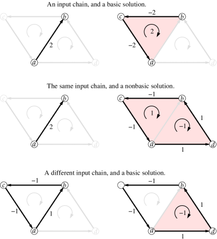
Figure 2: Simple examples of basic and nonbasic solutions.

Figure 2 illustrates nonbasic and basic solutions of the OHCP LP in a $2$-complex. Orientations of simplices in $K$, coefficients of the input chains, and the $p$- and $q$-coefficients of the solutions are shown. Note that the $p$-coefficients are the same for the second nonbasic solution and the last basic solution. Whether or not a solution is basic can depend on the $q$-coefficients and the input chain.

Consider the $2(m+n)\times(m+2n)$ matrix $\displaystyle N=\begin{bmatrix}I_{m}&&B\\ I_{m}\\ &I_{n}&I_{n}\\ &I_{n}\end{bmatrix}$ (entries not specified are zero). The columns of $N$ form a basis of $\operatorname{Ker}(A)$. Analyzing its structure, together with Theorem 3.3, yields the following results, whose proofs we omit.

Lemma 3.4.

Any basic solution of an OHCP LP is concise.

Lemma 3.5.

Any $\mathbf{z}^{K}\in\operatorname{Ker}(A)$ is equivalent to a linear combination of the last $n$ columns of $N$.

Corollary 3.6.

If $\mathbf{z}^{K}\in\left(\operatorname{Ker}(A)\setminus\{\mathbf{0}\}\right)$ is concise, then at least one $y$-coordinate in $\mathbf{z}^{K}$ is nonzero.

Lemma 3.7.

Let $\mathbf{z}\in P_{A}$ be a basic solution. Let $\mathbf{z}^{0}\in P_{A}$ with $\mathbf{z}^{0}$ concise in all $x$-entries. Let $\mathbf{z}=\mathbf{z}^{0}+\mathbf{z}^{K}$, with $\mathbf{z}^{K}$ being concise in all $x$-entries, and for each $y$-coordinate $j,z_{j}^{0}\neq 0\implies z_{j}\neq 0$. Then $\mathbf{z}^{K}\neq\mathbf{0}$ if and only if there exists a $p$-coefficient that is 0 in $\mathbf{z}$, but nonzero in $\mathbf{z}^{0}$.

Proof.

If there is a $p$-coefficient that is 0 in $\mathbf{z}$, but nonzero in $\mathbf{z}^{0}$, then $\mathbf{z}^{K}\neq\mathbf{0}$ simply because $\mathbf{z}=\mathbf{z}^{0}+\mathbf{z}^{K}$. Now assume $\mathbf{z}^{K}\neq\mathbf{0}$. Then $\mathbf{z}\neq\mathbf{z}^{0}$. Because $\mathbf{z}$ is basic, it is the only point in $P_{A}$ where all entries that are 0 at $\mathbf{z}$ are 0. Since for each $y$-coordinate $j,z_{j}^{0}\neq 0\implies z_{j}\neq 0$, there must be some $x$ entries that are zero at $\mathbf{z}$, but nonzero at $\mathbf{z}^{0}$. Let $i$ be one such entry. Since $i$ is 0 at $\mathbf{z}$ but nonzero at $\mathbf{z}^{0}$, it must be nonzero in $\mathbf{z}^{K}$. Since $\mathbf{z}^{0}$ and $\mathbf{z}^{K}$ are concise in all $x$-entries, $-i$ must be 0 in both $\mathbf{z}^{0}$ and $\mathbf{z}^{K}$, and therefore also at $\mathbf{z}$. Therefore the $p$-coefficient corresponding to $i$ and $-i$ must be 0 in $\mathbf{z}$ but nonzero in $\mathbf{z}^{0}$. ∎

For $p=1$, Lemma 3.7 is saying that if we attempt to get to a basic solution by adding a set of triangles to the input chain, then adding that set of triangles must completely cancel at least one edge. Referring to the two basic solutions shown in Figure 2, the edge of the input chain canceled is edge $ab$ in both cases.

Definition 3.8.

A set of vectors is linearly concise if any linear combination of the set is concise.

The next result establishes a method for decomposing a nonbasic solution into a basic solution and a remainder element of $\operatorname{Ker}(A)$, which we will use in later analysis.

Theorem 3.9.

Let $\mathbf{z}^{0}\in P_{A}$ be a basic solution. Let $\mathbf{z}^{K}\in\operatorname{Ker}(A)$ with $\{\mathbf{z}^{0},\mathbf{z}^{K}\}$ linearly concise. Let $\mathbf{z}=\mathbf{z}^{0}+\mathbf{z}^{K}$. Then $\mathbf{z}$ is a basic solution if and only if there do not exist $\mathbf{z}^{C},\mathbf{z}^{D}$ satisfying the following properties:

1. $\mathbf{z}^{C}+\mathbf{z}^{D}=\mathbf{z}^{K}$.

2. $\mathbf{z}^{C},\mathbf{z}^{D}\in\operatorname{Ker}(A)$.

3. $\mathbf{z}^{D}\neq\mathbf{0}$.

4. $\{\mathbf{z}^{0},\mathbf{z}^{K},\mathbf{z}^{D}\}$ is linearly concise.

5. $\mathbf{z}^{0}+\mathbf{z}^{C}=\mathbf{z}^{1}$ is a basic solution.

6. For each $y$-coordinate $j,z_{j}^{1}\neq 0\implies z_{j}\neq 0$.

7. For each $x$-coordinate $i,z_{i}^{D}\neq 0\implies z_{i}\neq 0$.

Proof.

Suppose there exists such a decomposition of $\mathbf{z}^{K}$. By Property 2, and that $\mathbf{z}^{0}\in P_{A}$, we have that $\mathbf{z}\in P_{A}$. Therefore if $\mathbf{z}$ is a basic solution, then the vectors $\mathbf{z},\mathbf{z}^{1},\mathbf{z}^{D}$ satisfy the conditions for $\mathbf{z},\mathbf{z}^{0},\mathbf{z}^{K}$ in Lemma 3.7. Because of Property 4, $\{\mathbf{z}^{0},\mathbf{z}^{K},\mathbf{z}^{C},\mathbf{z}^{D},\mathbf{z}^{1},\mathbf{z}\}$ is linearly concise. Therefore $\left(\forall x\text{-coordinate }i\right.$, $\left.z_{i}=z_{-i}\implies z_{i}^{1}=z_{-i}^{1}\right)$ $\iff$ $\left(\forall x\text{-coordinate }i\right.$, $z_{i}=0$ $\left.\implies z_{i}^{1}=0\right)$ $\iff$ $\left(\forall x\text{-coordinate }i\right.$, $z_{i}=0$ $\left.\implies z_{i}^{D}=0\right)$ $\iff$ $\left(\forall x\text{-coordinate }i\right.$, $z_{i}^{D}\neq 0\implies$ $\left.z_{i}\neq 0\right)$. So by Lemma 3.7, $\mathbf{z}$ is not a basic solution.

Now suppose $\mathbf{z}$ is not a basic solution. $\{\mathbf{z}^{0},\mathbf{z}^{K},\mathbf{z}\}$ is still linearly concise. Construct $\mathbf{z}^{D}$ and find $\mathbf{z}^{1}$ using the following algorithm.

1. Let $\mathbf{z}^{D}=\mathbf{0},\mathbf{z}^{1}=\mathbf{z}$. Then $\{\mathbf{z}^{0},\mathbf{z}^{K},\mathbf{z}^{D},\mathbf{z}^{1}\}$ is linearly concise.

2. $\mathbf{z}^{1}$ must be in $P_{A}$, and is not a basic solution. By Theorem 3.3, $\exists\,\mathbf{z}^{N}\in(\operatorname{Ker}(A)\setminus\{\mathbf{0}\})$ where $z_{i}^{N}\neq 0\implies z_{i}^{1}\neq 0$. Because $\{\mathbf{z}^{0},\mathbf{z}^{K},\mathbf{z}^{D},\mathbf{z}^{1}\}$ is linearly concise, $\{\mathbf{z}^{0},\mathbf{z}^{K},\mathbf{z}^{D},\mathbf{z}^{1},\mathbf{z}^{N}\}$ is linearly concise.

3. By Corollary 3.6, $z_{i}^{N}\neq 0$ for some $y$-coordinate $i$. Find $i$ such that $z_{j}^{N}\neq 0,j>2m\implies\lvert z_{i}^{1}/z_{i}^{N}\rvert\leq\lvert z_{j}^{1}/z_{j}^{N}\rvert$.

4. Let $\alpha=z_{i}^{1}/z_{i}^{N}$.

5. Let $\mathbf{z}^{D}=\mathbf{z}^{D}+\alpha\mathbf{z}^{N},\mathbf{z}^{1}=\mathbf{z}^{1}-\alpha\mathbf{z}^{N}$. Because we may add any linear combination of a set of linearly concise vectors to the linearly concise set, $\{\mathbf{z}^{0},\mathbf{z}^{K},\mathbf{z}^{D},\mathbf{z}^{1},\mathbf{z}^{N}\}$ is still linearly concise.

6. IF $\mathbf{z}^{1}$ is not a basic solution THEN LOOP to Step 2.

7. STOP.

Because $K$ is finite, and we make at least one $y$-entry zero that was nonzero in $\mathbf{z}^{1}$ in each loop, and do not make any zero $y$-entries in $\mathbf{z}^{1}$ nonzero. Hence by Theorem 3.3, this algorithm must eventually terminate. More precisely, it must terminate after at most $n$ iterations. By our criteria of choosing $\mathbf{z}^{N}$ in each loop, $\mathbf{z}^{D},\mathbf{z}^{1}$, and $\mathbf{z}^{C}=\mathbf{z}^{K}-\mathbf{z}^{D}$ satisfy all the criteria of the theorem. ∎

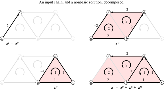
Figure 3: An illustration of $\mathbf{z}^{C}$ and $\mathbf{z}^{D}$.

The decomposition described in Theorem 3.9 isolates the portion(s) of a solution that makes it nonbasic. Figure 3 illustrates a simple example. At upper left is the input chain, equivalent to $\mathbf{z}^{I}$, and which takes the role of $\mathbf{z}^{0}$ in the theorem. Note that the illustration only shows equivalence classes under $p$- and $q$-coefficients. The next Lemma 3.10 describes necessary conditions to transform a nonbasic solution to a basic one.

Lemma 3.10.

Let $\mathbf{z}^{0}\in P_{A}$ be concise. Let $\mathbf{z}=\mathbf{z}^{0}+\mathbf{z}^{1}$ where $z_{j}^{0}\neq 0\implies z_{j}^{1}=0\ \forall j>2m$. If $\mathbf{z}$ is a basic solution in $P_{A}$, then for each $\mathbf{z}^{K}\in\left(\operatorname{Ker}(A)\setminus\{\alpha\mathbf{z}^{1}\}\right)\left(\alpha\in{\mathbb{R}}\right)$ where $z_{i}^{K}\neq 0\implies z_{i}^{0}\neq 0$, there must be two $x$-coordinates $r$ and $s$ where $z_{r}=z_{s}=0$, $z_{r}^{K},z_{s}^{K}\neq 0$, and $\displaystyle\frac{z_{r}^{K}}{z_{r}^{1}}\neq\frac{z_{s}^{K}}{z_{s}^{1}}$. Furthermore, if $O_{r}$ and $O_{s}$ are the OHCP LPs with input chains where the only nonzero coefficients are $r$ and $s$, respectively, with these coefficients equaling those in $\mathbf{z}^{0}$, then $\mathbf{z}^{1}+\mathbf{z}^{I\prime}$ is a basic solution to $O_{r}$ or $O_{s}$ where $\mathbf{z}^{I\prime}$ is the solution with $\{\mathbf{z}^{1},\mathbf{z}^{I\prime}\}$ linearly concise and equivalent to the identity solution for $O_{r}$ or $O_{s}$, respectively.

Proof.

By Theorem 3.3, the existence of $\mathbf{z}^{K}\in\left(\operatorname{Ker}(A)\setminus\{\alpha\mathbf{z}^{1}\}\right)$ where $z_{i}^{K}\neq 0\implies z_{i}^{0}\neq 0$, implies $\mathbf{z}^{0}$ is not a basic solution. Assume there is such a $\mathbf{z}^{K}$ with no such $r$ and $s$. By $z_{j}^{0}\neq 0\implies z_{j}^{1}=0\ \forall j>2m$, we get $z_{j}^{K}\neq 0\implies z_{j}\neq 0\ \forall j>2m$. So if there is no $x$-coordinate $r$ where $\mathbf{z}_{r}^{K}\neq 0,\mathbf{z}_{r}=0$, then $\mathbf{z}$ cannot be a basic solution. Let $\mathscr{R}$ be the set of $x$-coordinates where $\mathbf{z}_{r}^{K}\neq 0,\mathbf{z}_{r}=0$, and assume $\mathscr{R}$ is nonempty. Because there is no such $r$ and $s$, there is some $\alpha\in{\mathbb{R}}$ such that $(z_{r}^{K}/z_{r}^{1})=\alpha\ \forall r\in\mathscr{R}$. If $\mathbf{z}\in P_{A}$, then $\mathbf{z}^{1}\in\operatorname{Ker}(A)$. So then $\mathbf{z}^{K}-\alpha\mathbf{z}^{1}$ is in $\operatorname{Ker}(A)$, and $z_{i}=0\implies z_{i}^{K}-\alpha z_{i}^{1}=0\ \forall i\leq 2m$. Because $\mathbf{z}^{K}\neq\alpha\mathbf{z}^{1},\ \mathbf{z}^{K}-\alpha\mathbf{z}^{1}\neq\mathbf{0}$. Therefore by Theorem 3.3, $\mathbf{z}$ is not a basic solution.

Let $\mathbf{z}^{I\prime}$ be the solution with $\{\mathbf{z}^{1},\mathbf{z}^{I\prime}\}$ linearly concise and equivalent to the identity solution for $O_{r}$. If $\mathbf{z}^{I\prime}+\mathbf{z}^{1}$ is not a basic solution to $O_{r}$, then we may decompose $\mathbf{z}^{1}$ into $\mathbf{z}^{C}+\mathbf{z}^{D}$ according to Theorem 3.9. If $\mathbf{z}^{D}$ does not bring $z_{s}^{0}$ to zero in our original OHCP LP $O$, then $\mathbf{z}$ cannot be a basic solution of $O$ because all nonzero coefficients of $\mathbf{z}^{D}$ will be nonzero in $\mathbf{z}$. Even if it does bring $z_{s}^{0}$ to zero, $\mathbf{z}^{0}+\mathbf{z}^{C}$ cannot be a basic solution because of the first part of this lemma, and because $\mathbf{z}^{D}$ does not bring any coefficients of $\mathbf{z}^{C}$ to zero, by the first part of this Lemma, $\mathbf{z}^{0}+\mathbf{z}^{C}+\mathbf{z}^{D}$ cannot be a basic solution unless there is another $r$ and $s$ satisfying all qualities of the lemma. A symmetric argument holds replacing $r$ with $s$ and vice versa. ∎

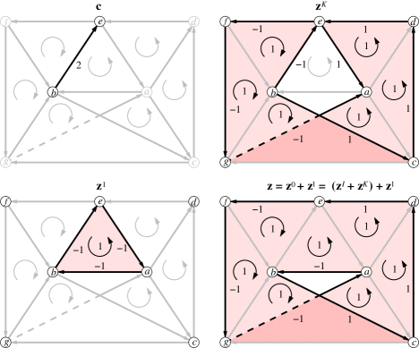
Figure 4: A Möbius strip illustrating Lemma 3.10.

We illustrate the Lemma in Figure 4. In this example, $r$ and $s$ correspond to the edges $be$ and $ea$, respectively, of $\mathbf{z}^{1}$. Note that both of these edges have coefficients of $-1$ in $\mathbf{z}^{1}$, but one has a coefficient of $1$ in $\mathbf{z}^{K}$. Therefore the inequality of the ratios specified in Lemma 3.10 holds; one ratio is $1$, and the other $-1$. Isolating the edges corresponding to $r$ and $s$ as inputs with coefficients taken from $\mathbf{z}^{0}$ will show that the other requirements of Lemma 3.10 are also met.

The remaining results of this section describe the relationship between the existence of (non)integral basic solutions of an OHCP LP, and the existence of (non)integral vertices.

Lemma 3.11.

Let $\mathbf{z}^{0}$ be concise. For any $\mathbf{z}$, there exists a $\mathbf{z}^{\prime}$ such that $\{\mathbf{z}^{\prime},\mathbf{z}^{0}\}$ is linearly concise, and $\mathbf{z}$ and $\mathbf{z}^{\prime}$ are equivalent.

Proof.

For each $i$ such that $z_{i}\neq 0,z_{-i}^{0}\neq 0$, subtract $z_{i}$ from both $z_{i}$ and $z_{-i}$. The result will be both equivalent to $\mathbf{z}^{\prime}$, and form a linearly concise set with $\mathbf{z}^{0}$. ∎

Lemma 3.12.

$\mathbf{z}$ is a basic solution if and only if $\mathbf{z}$ is concise, and each $\mathbf{z}^{\prime}$ that is concise and equivalent to $\mathbf{z}$ is a basic solution.

Proof.

Assume $\mathbf{z}$ is a basic solution. Then by Lemma 3.4, it is concise. For any $\mathbf{z}^{\prime}$ that is also concise and equivalent to $\mathbf{z}$, we transform $\mathbf{z}$ to $\mathbf{z}^{\prime}$ by taking each $z_{i}$ where $z_{i}\neq z_{i}^{\prime}$, and subtracting $z_{i}$ from both $z_{i}$ and $z_{-i}$. For each pair of subtractions, we make exactly one inequality constraint active, namely $z_{i}\geq 0$, and exactly one inactive, $z_{-i}\geq 0$. For any linearly independent set of constraints containing $z_{i}\geq 0$, if we replace this constraint with $z_{-i}\geq 0$, the result must again be a linearly independent set.

If each $\mathbf{z}^{\prime}$ that is concise and equivalent to $\mathbf{z}$ is a basic solution, and $\mathbf{z}$ is concise, then a similar logic holds to show $\mathbf{z}$ is a basic solution. ∎

Corollary 3.13.

If $\mathbf{z}$ is a basic solution, then there is a unique vertex $\mathbf{z}^{\prime}$ that is equivalent to $\mathbf{z}$.

Proof.

For each $i$ with $z_{i}<0$, subtract $z_{i}$ from both $z_{i}$ and $z_{-i}$. The result will be both concise and equivalent to $\mathbf{z}$, and so by Lemma 3.12 will be a basic solution. It will also be nonnegative, and therefore a vertex. Also for each $i$, there is one value we may add to both $z_{i}$ and $z_{-i}$ such that the result will be a vertex and equivalent to $\mathbf{z}$. ∎

Corollary 3.14.

Let $\mathbf{z}$ be concise. Then $\mathbf{z}$ is integral if and only if each $\mathbf{z}^{\prime}$ that is concise and equivalent to $\mathbf{z}$ is integral.

Proof.

We transform $\mathbf{z}$ to $\mathbf{z}^{\prime}$ using the same method as in Lemma 3.12. The result holds by the closure of integers under addition. ∎

4 Fractional Solutions to the OHCP LP, and Elementary Chains

Consider the special case of OHCP where the input chain $\mathbf{c}$ is the elementary $p$-chain $\mathbf{e}_{i}$ for some $i\leq m$, i.e., the $i{\text{th}}$ $p$-simplex has a coefficient of $1$ in the chain while all other entries are zero. We refer to this instance of the OHCP LP as OHCP_i, and its feasible region as $P_{i}$. We analyze the relationship between the existence of nonintegral values in basic solutions of the OHCP LP, and the existence of nonintegral values in a basic solution of OHCP_i for some $i$.

Lemma 4.1.

Let $\alpha\in\left({\mathbb{R}}\setminus\{0\}\right)$. $\mathbf{z}$ is a basic solution of the OHCP LP $O$ with input chain $\mathbf{c}$ if and only if $\alpha\mathbf{z}$ is a basic solution of the OHCP LP $O^{\prime}$ with input chain $\alpha\mathbf{c}$.

Proof.

If $\alpha\neq 0$, then multiplying $\mathbf{z}$ by $\alpha$ does not change which entries are nonzero. Therefore the set of active inequality constraints are the same at $\mathbf{z}$ and $\alpha\mathbf{z}$. And if we multiply both a solution and the input chain by the same scalar, the set of active equality constraints cannot change. Therefore the set of active constraints is the same for $\mathbf{z}$ in $O$ and for $\alpha\mathbf{z}$ in $O^{\prime}$. Therefore $\mathbf{z}$ is a basic solution to $O$ if and only if $\alpha\mathbf{z}$ is a basic solution to $O^{\prime}$. ∎

Theorem 4.2.

Let $\mathbf{z}\in P_{A}$ be a basic solution to the OHCP LP, with $\{\mathbf{z},\mathbf{z}^{I}\}$ linearly concise. There exists some matrix $Z$ such that the columns of $Z$ form a linearly concise set, each column $Z_{i}$ of $Z$ is a basic solution in $(P_{i})_{A}$, and $Z\mathbf{c}=\mathbf{z}$.

Proof.

Assume $\mathbf{z}$ is a basic solution in $P_{A}$. Begin constructing $Z$ by first setting each column $Z_{i}$ to the vector that is linearly concise with $\mathbf{z}^{I}$, and equivalent to the identity solution of OHCP_i. Then $Z\mathbf{c}=\mathbf{z}^{I}$. By Theorem 3.3 and Lemma 3.5, the identity solution to any OHCP LP is a basic solution. So by Lemma 3.12, each $Z_{i}$ is a basic solution to OHCP_i in $(P_{i})_{A}$. Also, by Lemma 4.1, $c_{i}Z_{i}$ is a basic solution to the OHCP LP with input chain $c_{i}\mathbf{e}_{i}$.

Let $\mathbf{z}^{K}=\mathbf{z}-\mathbf{z}^{I}$. If $\mathbf{z}^{K}\neq\mathbf{0}$, distribute it among the columns of $Z$ according to the following algorithm.

1. Let $\mathbf{z}^{0}$ = $\mathbf{z}^{I}$.

2. Since $\{\mathbf{z},\mathbf{z}^{0}\}$ is linearly concise, $\mathbf{z}^{K}$ is concise. By Lemma 3.7, there is some $x$-coordinate $i$ such that $z_{i}^{0}\neq 0,z_{i}=0$. It must also be true that $c_{i^{\prime}}\neq 0$ where $i^{\prime}$ is either $i$ or $-i$. Note that $Z_{i^{\prime}}$ is equal to $\begin{bmatrix}\mathbf{e}_{i^{\prime}}^{T}&\mathbf{0}^{T}&\mathbf{0}^{T}&\mathbf{0}^{T}\end{bmatrix}^{T}$.

3. IF $c_{i^{\prime}}Z_{i^{\prime}}+\mathbf{z}^{K}$ is not a solution to the OHCP LP with input chain $c_{i^{\prime}}\mathbf{e}_{i^{\prime}}$, THEN

   1. Construct $\mathbf{z}^{C}$ and $\mathbf{z}^{D}$ according to the algorithm in Theorem 3.9. Note that $\mathbf{z}^{0}$ and $\mathbf{z}^{K}$ represent the same vectors in Theorem 3.9 as they do here. However, the difference between $\mathbf{z}$ of this Lemma and $\mathbf{z}$ of Theorem  3.9 is $\mathbf{z}^{I}-c_{i^{\prime}}Z_{i^{\prime}}$.

   2. $\mathbf{z}^{C}$ cannot be $\mathbf{0}$. Otherwise, $\mathbf{z}^{D}$ would be $\mathbf{z}^{K}$, and so by our choice of $i$ in step 2, would not satisfy Property 7 of Theorem 3.9. Also recall from Theorem 3.9 that all vectors referred to in this algorithm form a linearly concise set. Add $\frac{1}{c_{i^{\prime}}}\mathbf{z}^{C}$ to $Z_{i^{\prime}}$.

   3. Set $\mathbf{z}^{K}:=\mathbf{z}^{D}$. By Property 3 of Theorem 3.9, we still have $\mathbf{z}^{K}\neq 0$.

   4. Set $\mathbf{z}^{0}:=\mathbf{z}^{0}+\mathbf{z}^{C}$. $\{\mathbf{z},\mathbf{z}^{0}\}$ is still linearly concise. And because $\mathbf{z}^{C}$ satisfies Property 6 of Theorem 3.9, we still have that for each $y$-coordinate $j,z_{j}^{0}\neq 0\implies z_{j}\neq 0$. Also, by Property 7, for any $x$-coordinate $i$ where $z_{i}^{0}\neq 0$ and $z_{i}=0,c_{i^{\prime}}\neq 0$ where $i^{\prime}$ is either $i$ or $-i$. This is because the only $x$-coefficients that are not zero in the $\mathbf{z}$ of Theorem 3.9, but are zero in the $\mathbf{z}$ of this theorem must be nonzero in $\mathbf{z}^{I}$.

   5. LOOP to Step 2. Note that the next $i$ chosen in Step 2 cannot be the same as any previous $i$s chosen, since by Lemma 3.7, and our previous choices of $i$, $z_{i}^{0}$ must be 0 for each previous $i$.

4. Add $\frac{1}{c_{i^{\prime}}}\mathbf{z}^{K}$ to $Z_{i^{\prime}}$.

5. STOP.

Because each $\mathbf{z}^{C}$ is nonzero, and $K$ is finite, this algorithm must terminate, giving us the desired $Z$. ∎

Consider the case of $p=1$. Because a basic solution $\mathbf{z}$ cannot be decomposed as in Theorem 3.9 the set of triangles of $\mathbf{z}$ form a union of 2D spaces each of which must be connected to at least one edge $\tau$ of the input chain $\mathbf{c}$. Then each of these 2D spaces must be a basic solution to the OHCP LP where $\tau$ has the only nonzero coefficient in the input chain $\mathbf{c}_{\tau}$, and the coefficient of $\tau$ is the same in $\mathbf{c}$ and $\mathbf{c}_{\tau}$. By Lemma 4.1, we may scale each of these basic solutions as necessary to be basic solutions of elementary chains. These basic solutions of elementary chains, adjusted as necessary to form a linearly concise set, are columns of $Z$. Note that the construction of $Z$ may not be unique, and many of the columns of $Z$ may be equivalent to identity solutions.

We may refer to Figure 2 and think of the edges of the last input chain as three different input chains consisting individually of $ab,bc$, and $ca$. We may then decompose the basic solution shown into solutions equivalent to identity solutions for $bc$ and $ca$, and a basic solution to $ab$.

Lemma 4.3.

For a given complex $K$, there is an OHCP LP with integral input chain $\mathbf{c}$ that has a nonintegral basic solution if and only if there is some $i$ such that the $i{\text{th}}$ coefficient is nonzero in $\mathbf{c}$, and OHCP_i has a nonintegral basic solution.

Proof.

If there is some $i$ such that OHCP_i has a nonintegral basic solution, then $\mathbf{e}_{i}$ is an integral input chain that has a nonintegral basic solution. If $\mathbf{z}$ is a nonintegral basic solution to the OHCP LP with integral input chain $\mathbf{c}$, then by Theorem 4.2, $\mathbf{z}$ is the sum of $n$ vectors each of the form $c_{i}\left(\mathbf{z}^{I}\right)_{\pm i}+\mathbf{z}^{C}$, where $\mathbf{z}^{C}\neq\mathbf{0}\implies c_{i}\neq 0$. Since integers are closed under addition, one of these terms must be nonintegral. Since $c_{i}$ and $\left(\mathbf{z}^{I}\right)_{\pm i}$ both must be integral, there must be some $\mathbf{z}^{C}$ that is nonintegral. Therefore some $\frac{1}{c_{i}}\mathbf{z}^{C}$ is also nonintegral, and so $\left(\mathbf{z}^{I}\right)_{\pm i}+\frac{1}{c_{i}}\mathbf{z}^{C}$ is nonintegral. By Theorem 4.2, each $\left(\mathbf{z}^{I}\right)_{\pm i}+\frac{1}{c_{i}}\mathbf{z}^{C}$ is a basic solution to OHCP_i. Therefore some $\left(\mathbf{z}^{I}\right)_{\pm i}+\frac{1}{c_{i}}\mathbf{z}^{C}$ is a nonintegral basic solution to OHCP_i. Furthermore, the $i{\text{th}}$ coefficient of $\mathbf{c}$ must be nonzero, otherwise this sum is undefined. ∎

Lemma 4.4.

Let $\mathbf{z}^{0}$ be concise and be in the hyperplane $P_{A}$ of the OHCP $O$ with input chain $\mathbf{c}$, with $\mathbf{z}$ a basic solution to the same OHCP in $P_{A}$ where for each $y$-coordinate $j,z_{j}=0\implies z_{j}^{0}=0$. Let $\mathbf{y}^{0}$ be the $2(m+n)$-vector with all $y$-coefficients equal to those of $\mathbf{z}^{0}$, and all $x$-coefficients 0. Then $\mathbf{z}-\mathbf{y}^{0}$ is a basic solution of the OHCP $O^{0}$ with input chain $\mathbf{c}^{0}$ in $(P_{A})^{0}$ where $[\left(\mathbf{c}^{0}\right)^{T}\mathbf{0}^{T}]^{T}$ is equivalent in all $x$-coordinates to $\mathbf{z}^{0}$.

Proof.

Since $\mathbf{z}$ and $\mathbf{z}^{0}$ are both in $P_{A}$, the difference between them is in $\operatorname{Ker}(A)$. Since $[\left(\mathbf{c}^{0}\right)^{T}\mathbf{0}^{T}]^{T}$ and $\mathbf{z}^{0}$ are equivalent in all $x$-coordinates, $\mathbf{z}^{0}-\mathbf{y}^{0}$ is equivalent to the identity solution for $O^{0}$. Therefore $\mathbf{z}^{0}-\mathbf{y}^{0}$ and $\mathbf{z}-\mathbf{y}^{0}$ are both in $(P_{A})^{0}$.

We show that $\mathbf{z}-\mathbf{y}^{0}$ is a basic solution of $O^{0}$ by contrapositive. Let $\mathbf{z}^{*}$ represent $\mathbf{z}-\mathbf{y}^{0}$. Suppose $\mathbf{z}^{*}$ is not a basic solution of $O^{0}$. Then by Theorem 3.3, $\exists\mathbf{z}^{K}\in\left(\operatorname{Ker}(A)\setminus\{\mathbf{0}\}\right)$ where $z_{i}^{*}=0\implies z_{i}^{K}=0.\ \mathbf{z}$ and $\mathbf{z}^{*}$ agree in all $x$-coordinates. We also have for each $y$-coordinate $j,z_{j}=0\implies z_{j}^{0}=0\implies y_{j}^{0}=0\implies z_{j}^{*}=0\implies z_{j}^{K}=0$. Therefore we have $z_{i}=0\implies z_{i}^{K}=0$ for all $i$. Therefore by Theorem 3.3, $\mathbf{z}$ is not a basic solution of $O$. ∎

For $p=1$, due to Corollary 3.13, Lemma 4.4 is saying that if we have a set of edges $\mathbf{x}$ that is a vertex for some OHCP LP with input chain $\mathbf{c}$, and we transform $\mathbf{c}$ to $\mathbf{x}$ by adding triangles one at a time, or at least not eliminating triangles previously added, then $\mathbf{x}$ will be a vertex to any OHCP LP that has as input any of these intermediate edge sets we get at each step of this transformation.

Lemma 4.5.

For a given complex $K$, there is an OHCP LP with integral input chain $\mathbf{c}$ that has a nonintegral basic solution if and only if there is some $i$ such that OHCP_i has a basic solution where all $y$-coordinates that are nonzero are nonintegral.

Proof.

Let $\mathbf{z}$ be a basic solution with nonintegral coefficients for an OHCP LP with integral input chain $\mathbf{c}$. By Theorem 4.2, there is some matrix $Z$ such that the columns of $Z$ form a linearly concise set, each column $Z_{i}$ of $Z$ is a basic solution in $(P_{i})_{A}$, and $Z\mathbf{c}=\mathbf{z}$. By a similar logic as Lemma 4.3, one of these columns is nonintegral, and this column is of the form $\left(\mathbf{z}^{I}\right)_{\pm i}+\frac{1}{c_{i}}\mathbf{z}^{C}$. For this $\mathbf{z}^{C}$, let $\mathscr{J}$ be the set of $y$-coordinates with nonzero integral coefficients in $\frac{1}{c_{i}}\mathbf{z}^{C}$.

If $\mathscr{J}$ is empty, then we have our desired result. If $\mathscr{J}$ is nonempty, decompose $\mathbf{z}^{C}$ into its linear combination of basis vectors of $\operatorname{Ker}(A)$ that are equivalent to the last $n$ columns of the matrix $N$ of Lemma 3.5. Let $\mathbf{z}^{0}$ be the sum of $\mathbf{e}_{\pm i}$ and the components of this linear combination with nonzero element in $\mathscr{J}$. Note that $\mathbf{z}^{0}$ is integral. Let $\mathbf{c}^{0}$ be the input chain where $[\left(\mathbf{c}^{0}\right)^{T}\mathbf{0}^{T}]^{T}$ is equivalent in all $x$-coordinates to $\mathbf{z}^{0}$. Let $\mathbf{y}^{0}$ be the $2(m+n)$-vector such that $j\in\mathscr{J}\implies y_{j}^{0}=(1/c_{i})z_{j}^{C},j\notin\mathscr{J}\implies y_{j}^{0}=0$. Then by Lemma 4.4, $\left(\mathbf{z}^{I}\right)_{\pm i}+(1/c_{i})\mathbf{z}^{C}-\mathbf{y}^{0}$ is a basic solution to the OHCP LP $O^{0}$ with input chain $\mathbf{c}^{0}$, and all of its nonzero $y$-coefficients are nonintegral.

Now let $\mathbf{z}=\left(\mathbf{z}^{I}\right)_{\pm i}+(1/c_{i})\mathbf{z}^{C}-\mathbf{y}^{0}$, let $\mathbf{c}=\mathbf{c}^{0}$, and apply the same logic as above. Note that with each iteration of this process, we lessen the number of nonzero $y$-coefficients; the set of nonzero $y$-coefficients of $\mathbf{z}$ contains the set of nonzero $y$-coefficients in $(1/c_{i})\mathbf{z}^{C}$, and this set decreases in size each round. Because $K$ is finite, this process must eventually terminate. ∎

Remark 4.6.

Lemmas 4.3 and 4.5 allow us to concentrate on the easier to analyze case of elementary input chains for the OHCP LP in order to arrive at our main results.

5 Projections Onto the Space of $p$-Simplex Coefficients

Call the space of $x$-variables $\mathscr{X}\left(={\mathbb{R}}^{2m}\right)$. We study the projections of the OHCP LP, $P,P_{A},\operatorname{Ker}(A),$ basic solutions, and vertices onto $\mathscr{X}$. For any of these objects $\Omega$, let $\Omega\arrowvert_{\mathscr{X}}$ represent the projection of $\Omega$ onto $\mathscr{X}$. Since the $y$-variables do not appear in the OHCP LP objective function, a vertex of $P\arrowvert_{\mathscr{X}}$ must be optimal. We establish correspondences between the basic solutions in the projection space and those in the original space. We then prove equivalent relationships between OHCP and OHCP_i in the projection space.

First, we extend the definition of concise to $(2m)$-vectors in the natural way. We also rephrase the definition of a basic solution below.

Definition 5.1.

Let $\mathscr{C}$ be the set of constraints of an OHCP LP $O$ that are not orthogonal to $\mathscr{X}$, i.e., the set of constraints with a nonzero $x$-coefficient. For any $\mathbf{x}\in\mathscr{X}$, let $\mathscr{C}_{\mathbf{x}}$ be the set of elements of $\mathscr{C}$ active at $\mathbf{x}$. Then $\mathbf{x}$ is a basic solution of $O\arrowvert_{\mathscr{X}}$ if and only if there is no other point in $\mathscr{X}$ where all elements of $\mathscr{C}_{\mathbf{x}}$ are active.

Note that if $\mathbf{x}$ fails Definition 5.1, then $\mathscr{C}_{\mathbf{x}}$ must be active for an entire affine space of some dimension $d\geq 1$. To say $\mathbf{x}\in X$ is feasible in $O\arrowvert_{\mathscr{X}}$ is equivalent to saying $\mathbf{x}\in P\arrowvert_{\mathscr{X}}$. We justify Definition 5.1 and how it relates to vertices of $P\arrowvert_{\mathscr{X}}$ with the following lemma.

Lemma 5.2.

$\mathbf{x}\in\mathscr{X}$ is a basic feasible solution of $O\arrowvert_{\mathscr{X}}$ if and only if $\mathbf{x}$ is feasible, and not a convex combination of any two distinct elements of $P\arrowvert_{\mathscr{X}}$.

Proof.

We prove both directions by contrapositive. If $\mathbf{x}$ is infeasible, then clearly it is not a basic feasible solution. Suppose $\mathbf{x}$ is a convex combination of two distinct elements $\mathbf{x}^{1}$ and $\mathbf{x}^{2}$ of $P\arrowvert_{\mathscr{X}}$. Then $\mathbf{x}=\lambda\mathbf{x}^{1}+(1-\lambda)\mathbf{x}^{2}$ for some $\lambda\in(0,1)$. Since $\mathbf{x}^{1},\mathbf{x}^{2}\in P\arrowvert_{\mathscr{X}}$, they are nonnegative, and so the set of nonzero coefficients of $\mathbf{x}$ is the union of the sets nonzero coefficients of $\mathbf{x}^{1}$ and $\mathbf{x}^{2}$. Therefore any inequality constraints in $\mathscr{C}$ active at $\mathbf{x}$ must also be active at $\mathbf{x}^{1}$ and $\mathbf{x}^{2}$. Since $P$ is convex, $P\arrowvert_{\mathscr{X}}$ is convex. Since $\mathbf{x}^{1},\mathbf{x}^{2}\in P\arrowvert_{\mathscr{X}},\mathbf{x}\in P\arrowvert_{\mathscr{X}}$. Therefore all equality constraints are active at all three points. Therefore $\mathbf{x}$ does not satisfy Definition 5.1 as a basic solution of $O\arrowvert_{\mathscr{X}}$.

Now suppose $\mathbf{x}$ is feasible, but does not satisfy the conditions specified in Definition 5.1. Let $\mathbf{x}^{\prime}$ be another point in $\mathscr{X}$ where all elements of $\mathscr{C}_{\mathbf{x}}$ are active. All equality constraints are active at $\mathbf{x}$, and so are also active at $\mathbf{x}^{\prime}$. Therefore $\mathbf{x}^{\prime}\in\left(P\arrowvert_{\mathscr{X}}\right)_{A}$. Let $L$ be the line in $\mathscr{X}$ containing $\mathbf{x}$ and $\mathbf{x}^{\prime}$. Then $L\subset\left(P\arrowvert_{\mathscr{X}}\right)_{A}$. Any point in $L$ may be expressed as $\alpha\mathbf{x}^{\prime}+(1-\alpha)\mathbf{x}$ for some $\alpha\in{\mathbb{R}}$. Choosing a value for $\alpha$ defines a point. Because $P\arrowvert_{\mathscr{X}}$ is convex, there is at most two values for $\alpha$ such that $\alpha\mathbf{x}^{\prime}+(1-\alpha)\mathbf{x}$ is on the boundary of $P\arrowvert_{\mathscr{X}}$. Since $\mathbf{x}$ is defined by $\alpha=0$, and $\mathbf{x}$ is feasible, at most one such value is positive, and at most one such value is negative.

If there is no such value for $\alpha$, then $L\subset P\arrowvert_{\mathscr{X}}$. Then choose values 1 and $-1$ for $\alpha$, to define $\mathbf{x}^{1}$ and $\mathbf{x}^{2}$. If there is only one such value $\alpha$, then choose $\alpha$ and $-\alpha$ to define $\mathbf{x}^{1}$ and $\mathbf{x}^{2}$. If there are two such values $\alpha_{1},\alpha_{2}$, then choose $\min\{\lvert\alpha_{1}\rvert,\lvert\alpha_{2}\rvert\}$ and $-\left(\min\{\lvert\alpha_{1}\rvert,\lvert\alpha_{2}\rvert\}\right)$ to define $\mathbf{x}^{1}$ and $\mathbf{x}^{2}$. In any case, both $\mathbf{x}^{1}$ and $\mathbf{x}^{2}$ are in $P\arrowvert_{\mathscr{X}}$, and $\mathbf{x}=(1/2)\mathbf{x}^{1}+(1/2)\mathbf{x}^{2}$. ∎

Lemma 5.2 shows we may define vertices of $P\arrowvert_{\mathscr{X}}$ the same way as in $P$. We now show results for basic solutions of $O\arrowvert_{\mathscr{X}}$ and vertices of $P\arrowvert_{\mathscr{X}}$ that parallel many of our previous results. Proofs are omitted where the logic is a natural parallel of these previous results.

Corollary 5.3.

Let $\mathbf{x}\in\left(P_{A}\right)\arrowvert_{\mathscr{X}}$. $\mathbf{x}$ is a basic solution of $O\arrowvert_{\mathscr{X}}$ if and only if $\,\forall\mathbf{x}^{K}\in\left(\operatorname{Ker}(A)\arrowvert_{\mathscr{X}}\setminus\{\mathbf{0}\}\right),\ \exists i:x_{i}=0,x_{i}^{K}\neq 0.$

Lemma 5.4.

Any basic solution $\mathbf{x}$ of $O\arrowvert_{\mathscr{X}}$ is concise.

A significant difference between the basic solutions in the projection space and those in the original space is that in the projection, because they are determined only by $p$-coefficients, the choice of input chain on a complex has no impact on whether or not a solution in $\left(P_{A}\right)\arrowvert_{\mathscr{X}}$ is basic in the projection. Referring back to Figure 2, the last solution is not basic in the projection. Lemma 5.5 formalizes this idea of the input chain not mattering, with some added context useful for our main result. It is a parallel to Lemma 4.4, but becomes simpler in the projection space.

Lemma 5.5.

Let $\mathbf{z}^{0}$ be concise and be in the hyperplane $P_{A}$ of the OHCP $O$ with input chain $\mathbf{c}$, with $\mathbf{z}$ a basic solution to the same OHCP in $P_{A}$ and $\mathbf{z}\arrowvert_{\mathscr{X}}$ a basic solution to $O\arrowvert_{\mathscr{X}}$. Then $\mathbf{z}\arrowvert_{\mathscr{X}}$ is a basic solution of the OHCP $O^{0}\arrowvert_{\mathscr{X}}$ with input chain $\mathbf{c}^{0}$ in $(P_{A})^{0}\arrowvert_{\mathscr{X}}$ where $[\left(\mathbf{c}^{0}\right)^{T}\mathbf{0}^{T}]^{T}$ is equivalent to $\mathbf{z}^{0}\arrowvert_{\mathscr{X}}$.

Proof.

Since $\mathbf{z}$ an $\mathbf{z}^{0}$ are both in $P_{A}$, the difference between them is in $\operatorname{Ker}(A)$. Since $[\left(\mathbf{c}^{0}\right)^{T}\mathbf{0}^{T}]^{T}$ and $\mathbf{z}^{0}$ are equivalent in all $x$-coordinates, $\mathbf{z}^{0}\arrowvert_{\mathscr{X}}$ is equivalent to the identity solution for $O^{0}$. Therefore $\mathbf{z}^{0}\arrowvert_{\mathscr{X}}$ and $\mathbf{z}\arrowvert_{\mathscr{X}}$ are both in $(P_{A})^{0}\arrowvert_{\mathscr{X}}$.

We show that $\mathbf{z}\arrowvert_{\mathscr{X}}$ is a basic solution of $O^{0}\arrowvert_{\mathscr{X}}$ by contrapositive. Let $\mathbf{x}=\mathbf{z}\arrowvert_{\mathscr{X}}$. Suppose $\mathbf{x}$ is not a basic solution of $O^{0}\arrowvert_{\mathscr{X}}$. Then by Corollary 5.3, $\exists\mathbf{x}^{K}\in\left(\operatorname{Ker}(A)\arrowvert_{\mathscr{X}}\setminus\{\mathbf{0}\}\right)$ where $x_{i}=0\implies x_{i}^{K}=0$. But then by Corollary 5.3, $\mathbf{z}\arrowvert_{\mathscr{X}}$ is not a basic solution of $O\arrowvert_{\mathscr{X}}$. ∎

Lemma 5.6.

For any basic solution $\mathbf{x}\in\left(P_{A}\right)\arrowvert_{\mathscr{X}}$ of $O\arrowvert_{\mathscr{X}}$, there is a basic solution $\mathbf{z}\in P_{A}$ of $O$ where $\mathbf{z}\arrowvert_{\mathscr{X}}=\mathbf{x}$.

Proof.

Since $\mathbf{x}\in\left(P_{A}\right)\arrowvert_{\mathscr{X}}$, there is some $\mathbf{z}^{\prime}$ where $\mathbf{z}^{\prime}\arrowvert_{\mathscr{X}}=\mathbf{x}$, and $\mathbf{z}^{\prime}\in P_{A}$. Since $\mathbf{z}^{\prime}$ and $\mathbf{x}$ agree in all $x$-variables and $\mathbf{x}$ is a basic solution, for any $\mathbf{z}^{K}$ where $z_{i}=0\implies z_{i}^{K}=0,\mathbf{z}^{K}\arrowvert_{\mathscr{X}}$ must be $\mathbf{0}$. If such a $\mathbf{z}^{K}$ exists, we may use the algorithm of Theorem 3.9 to arrive at a basic solution $\mathbf{z}$ of $O$ in $P_{A}$ where $\mathbf{z}\arrowvert_{\mathscr{X}}=\mathbf{x}$. ∎

Corollary 5.7.

If for a given complex $K$, all vertices of any OHCP LP are integral, then all vertices of any projection of an OHCP LP onto $\mathscr{X}$ must be integral.

Proof.

We prove by contrapositive. If there exists some $O\arrowvert_{\mathscr{X}}$ with a nonintegral vertex $\mathbf{x}$, then by Lemma 5.6 and Corollary 3.13, there is a vertex $\mathbf{z}$ of $O$ where all $x$-coordinates of $\mathbf{z}$ and $\mathbf{x}$ agree. Therefore $\mathbf{z}$ is nonintegral. ∎

Corollary 5.8.

Let $\mathbf{x}\in\left(P_{A}\right)\arrowvert_{\mathscr{X}}$ be a basic solution of $O\arrowvert_{\mathscr{X}}$. Let $\mathbf{x}^{0}\in\left(P_{A}\right)\arrowvert_{\mathscr{X}}$ with $\mathbf{x}^{0}$ concise. Let $\mathbf{x}=\mathbf{x}^{0}+\mathbf{x}^{K}$, with $\mathbf{x}^{K}$ being concise. Then $\mathbf{x}^{K}\neq\mathbf{0}$ if and only if there exists a $p$-coefficient that is zero in $\mathbf{x}$, but nonzero in $\mathbf{x}^{0}$.

Corollary 5.9.

Let $\mathbf{x}^{0}\in\left(P_{A}\right)\arrowvert_{\mathscr{X}}$ be a basic solution of $O\arrowvert_{\mathscr{X}}$. Let $\mathbf{x}^{K}\in\operatorname{Ker}(A)\arrowvert_{\mathscr{X}}$ with $\{\mathbf{x}^{0},\mathbf{x}^{K}\}$ linearly concise. Let $\mathbf{x}=\mathbf{x}^{0}+\mathbf{x}^{K}$. Then $\mathbf{x}$ is a basic solution if and only if there do not exist $\mathbf{x}^{C},\mathbf{x}^{D}$ satisfying the following properties:

1. $\mathbf{x}^{C}+\mathbf{x}^{D}=\mathbf{x}^{K}$.

2. $\mathbf{x}^{C},\mathbf{x}^{D}\in\operatorname{Ker}(A)\arrowvert_{\mathscr{X}}$.

3. $\mathbf{x}^{D}\neq\mathbf{0}$.

4. $\{\mathbf{x}^{0},\mathbf{x}^{K},\mathbf{x}^{D}\}$ is linearly concise.

5. $\mathbf{x}^{0}+\mathbf{x}^{C}=\mathbf{x}^{1}$ is a basic solution to $O\arrowvert_{\mathscr{X}}$.

6. $x_{i}^{D}\neq 0\implies x_{i}\neq 0\ \forall i$.

Proof.

We prove both directions again by contrapositive. The first direction follows in the same way as Theorem 3.9, replacing $\mathbf{z}$ with $\mathbf{x}$ and Lemma 3.7 with Corollary 5.8. Then suppose $\mathbf{x}$ is not a basic solution. $\{\mathbf{x}^{0},\mathbf{x}^{K},\mathbf{x}\}$ is still linearly concise. Construct $\mathbf{x}^{D}$ and find $\mathbf{x}^{1}$ using the following algorithm.

1. Let $\mathbf{x}^{D}=\mathbf{0},\mathbf{x}^{1}=\mathbf{x}$. Then $\{\mathbf{x}^{0},\mathbf{x}^{K},\mathbf{x}^{D},\mathbf{x}^{1}\}$ is linearly concise.

2. $\mathbf{x}^{1}$ must be in $\left(P_{A}\right)\arrowvert_{\mathscr{X}}$, and is not a basic solution. By Corollary 5.3, $\exists\,\mathbf{z}^{N}\in(\operatorname{Ker}(A)\arrowvert_{\mathscr{X}}\setminus\{\mathbf{0}\})$ where $x_{i}^{N}\neq 0\implies x_{i}^{1}\neq 0$. Because $\{\mathbf{x}^{0},\mathbf{x}^{K},\mathbf{x}^{D},\mathbf{x}^{1}\}$ is linearly concise, $\{\mathbf{x}^{0},\mathbf{x}^{K},\mathbf{x}^{D},\mathbf{x}^{1},\mathbf{x}^{N}\}$ is linearly concise.

3. Find $i$ such that $x_{j}^{N}\neq 0\implies\lvert x_{i}^{1}/x_{i}^{N}\rvert\leq\lvert x_{j}^{1}/x_{j}^{N}\rvert$.

4. Let $\alpha=x_{i}^{1}/x_{i}^{N}$.

5. Let $\mathbf{x}^{D}=\mathbf{x}^{D}+\alpha\mathbf{x}^{N},\mathbf{x}^{1}=\mathbf{x}^{1}-\alpha\mathbf{x}^{N}$. Because we may add any linear combination of a set of linearly concise vectors to the linearly concise set, $\{\mathbf{x}^{0},\mathbf{x}^{K},\mathbf{x}^{D},\mathbf{x}^{1},\mathbf{x}^{N}\}$ is still linearly concise.

6. IF $\mathbf{x}^{1}$ is not a basic solution of $O\arrowvert_{\mathscr{X}}$ THEN LOOP to Step 2.

7. STOP.

Because $K$ is finite, and we make at least one entry zero that was nonzero in $\mathbf{x}^{1}$ in each loop, and do not make any zero entries in $\mathbf{x}^{1}$ nonzero, then by Corollary 5.3, this algorithm must eventually terminate after at most $m$ iterations. And as in Theorem 3.9, $\mathbf{x}^{D},\mathbf{x}^{1}$, and $\mathbf{x}^{C}=\mathbf{x}^{K}-\mathbf{x}^{D}$ satisfy all criteria of the Corollary. ∎

Corollary 5.10.

Let $\mathbf{x}^{0}\in\left(P_{A}\right)\arrowvert_{\mathscr{X}}$ be concise. Let $\mathbf{x}=\mathbf{x}^{0}+\mathbf{x}^{1}$. If $\mathbf{x}$ is a basic solution in $\left(P_{A}\right)\arrowvert_{\mathscr{X}}$, then for each $\mathbf{x}^{K}\in\left(\operatorname{Ker}(A)\arrowvert_{\mathscr{X}}\setminus\{\alpha\mathbf{x}^{1}\}\right)$ for $\alpha\in{\mathbb{R}}$, where $x_{i}^{K}\neq 0\implies x_{i}^{0}\neq 0$, there must be two coordinates $r$ and $s$ where $x_{r}=x_{s}=0$, $x_{r}^{K},x_{s}^{K}\neq 0$, and $\displaystyle(x_{r}^{K}/x_{r}^{1})\neq(x_{s}^{K}/x_{s}^{1})$. Furthermore, if $\left(O_{r}\right)\arrowvert_{\mathscr{X}}$ and $\left(O_{s}\right)\arrowvert_{\mathscr{X}}$ are the projections of OHCP LPs with input chains where the only nonzero coefficients are $r$ and $s$ respectively, with these coefficients equaling those in $\mathbf{x}^{0}$, then $\mathbf{x}^{1}+\mathbf{x}^{I\prime}$ is a basic solution to $\left(O_{r}\right)\arrowvert_{\mathscr{X}}$ and $\left(O_{s}\right)\arrowvert_{\mathscr{X}}$ where $\mathbf{x}^{I\prime}$ is the solution with $\{\mathbf{x}^{1},\mathbf{x}^{I\prime}\}$ linearly concise and equivalent to the identity solution for $\left(O_{r}\right)\arrowvert_{\mathscr{X}}$ and $\left(O_{s}\right)\arrowvert_{\mathscr{X}}$, respectively.

Corollary 5.11.

$\mathbf{x}$ is a basic solution of $O\arrowvert_{\mathscr{X}}$ if and only if $\mathbf{x}$ is concise, and each $\mathbf{x}^{\prime}$ that is concise and equivalent to $\mathbf{x}$ is a basic solution.

Corollary 5.12.

For each basic solution $\mathbf{x}$ of $O\arrowvert_{\mathscr{X}}$, there is a unique vertex $\mathbf{x}^{\prime}$ of $O\arrowvert_{\mathscr{X}}$ that is equivalent to $\mathbf{x}$.

Corollary 5.13.

Let $\mathbf{x}$ be a concise solution of $O\arrowvert_{\mathscr{X}}$. Then $\mathbf{x}$ is integral if and only if each solution $\mathbf{x}^{\prime}$ of $O\arrowvert_{\mathscr{X}}$ that is concise and equivalent to $\mathbf{x}$ is integral.

Theorem 5.14.

For a given complex $K$, there is a nonintegral vertex $\mathbf{z}$ of some OHCP LP $O$ with integral input chain $\mathbf{c}$ where $\mathbf{z}\arrowvert_{\mathscr{X}}$ is a vertex of $P\arrowvert_{\mathscr{X}}$ if and only if there is some $i$ such that OHCP_i has a nonintegral vertex $\mathbf{z}^{\prime}$ such that $\mathbf{z}^{\prime}\arrowvert_{\mathscr{X}}$ is a vertex of $P_{i}\arrowvert_{\mathscr{X}}$ where the $i{\text{th}}$ coefficient of $\mathbf{c}$ is nonzero.

Proof.

One direction of the if and only if is trivially true: if there is some $i$ and OHCP_i, then the more general case of OHCP LP follows immediately. We prove the other direction by contrapositive. If there is no such $i$ where OHCP_i has a nonintegral vertex $\mathbf{z}^{\prime}$, then by Lemma 4.3 and Corollary 3.13, there can be no nonintegral vertex $\mathbf{z}$ of any OHCP LP.

Now suppose there is an $i$ where OHCP_i has a nonintegral vertex $\mathbf{z}^{\prime}$, but no such $i$ where $\mathbf{z}^{\prime}\arrowvert_{\mathscr{X}}$ is a vertex of $P_{i}\arrowvert_{\mathscr{X}}$. Then for any nonintegral vertex $\mathbf{z}$ of an OHCP LP, by Theorem 4.2 and Lemma 4.3, some column $\mathbf{z}^{\prime}$ of $Z$ with $Z\mathbf{c}=\mathbf{z}$ is a nonintegral basic solution of OHCP_i for some $i$. If we construct $Z$ using the algorithms of Theorem 4.2 and Theorem 3.9, then by Condition 7 of Theorem 3.9, any nonzero $p$-coefficient of $\mathbf{z}^{\prime}$ is nonzero in $\mathbf{z}$.

Since $\mathbf{z}^{\prime}\arrowvert_{\mathscr{X}}$ cannot be a vertex, it cannot be a basic solution of OHCP${}_{i}\arrowvert_{\mathscr{X}}$. So by Corollary 5.9, there is some $\mathbf{x}^{D}\in\operatorname{Ker}(A)\arrowvert_{\mathscr{X}}$ where every nonzero coefficient of $\mathbf{x}^{D}$ is nonzero in $\mathbf{z}^{\prime}\arrowvert_{\mathscr{X}}$. Since all these coefficients are $p$-coefficients, all the nonzero coefficients of $\mathbf{x}^{D}$ are nonzero in $\mathbf{z}\arrowvert_{\mathscr{X}}$. So by Corollary 5.9, $\mathbf{z}\arrowvert_{\mathscr{X}}$ cannot be a basic solution to $O\arrowvert_{\mathscr{X}}$, and so is not a vertex of $P\arrowvert_{\mathscr{X}}$. ∎

Corollary 5.15.

For a given complex $K$, there is an OHCP LP with integral input chain $\mathbf{c}$ that has a nonintegral vertex $\mathbf{z}$ where $\mathbf{z}\arrowvert_{\mathscr{X}}$ is a vertex of $P\arrowvert_{\mathscr{X}}$ if and only if there is some $i$ such that OHCP_i has a nonintegral vertex $\mathbf{z}^{\prime}$ with all nonzero $y$-coefficients nonintegral where $\mathbf{z}^{\prime}\arrowvert_{\mathscr{X}}$ is a vertex of $P_{i}\arrowvert_{\mathscr{X}}$.

Proof.

The result follows from Lemmas 4.5 and 5.5, and Corollaries 3.13, 3.14, 5.12, and 5.13. ∎

6 Minimally Non Totally-Unimodular Submatrices of $[\partial_{q}]$

We study minimal violations of total unimodularity, and describe a stricter version of a minimal violation submatrix of the boundary matrix. Intuitively, we study Möbius strips that do not contain smaller Möbius strips within their triangles. A minimally non totally-unimodular (MNTU) matrix is a matrix $M$ that is not totally unimodular, but every proper submatrix of $M$ is totally unimodular (also referred to as almost totally unimodular matrices [1]). Several properties of an MNTU matrix $M$ are known previously [1, 24].

1. A matrix is not totally unimodular if and only if has an MNTU submatrix $M$.

2. $\det(M)=\pm 2$.

3. Every column and every row of $M$ has an even number of nonzero entries, i.e., $M$ is Eulerian.

4. The sum of the entries of $M$ is $2\bmod 4$.

5. The bipartite graph representation of $M$ is a chordless (i.e., induced) circuit [8].

The bipartite graph representation [1, 8] a submatrix $M$ of $[\partial_{q}]$ has a vertex for each row and for each column of $M$, and an undirected edge for each nonzero entry $M_{ij}$ connecting the vertices for row $i$ and column $j$. Notice that each edge connects a row vertex, or $p$-vertex, with a column vertex, or $q$-vertex. A circuit $C$ in a weighted graph is b-odd (b-even) if the sum of the weights of the edges in $C$ is $2\bmod 4$ ($0\bmod 4$). The quality of $C$ being b-even, b-odd, or neither is called the b-parity of $C$. The following theorem characterizes this bipartite graph as a circuit.

Theorem 6.1.

Given a circuit $C$ that is the bipartite graph representation of an MNTU submatrix $M$ of $[\partial_{q}]$, and a set of flags placed on an arbitrary subset of the $q$-vertices of $C$, there exists a traversal of $C$ such that each portion of the traversal of $C$ between two consecutive flags is induced.

Proof.

Recall that for any circuit $C$, if an edge $h\in C$ is a potential chord of a subgraph of $C$, then both of its end points are of degree $4$ or more in $C$. If there is no path in $C$ between two flags, then every path between them must contain both end points of a chord, and we have a set of paths like one of the graphs in Figure 5. The graphs shown are abstractions of $C$ in the case where the end points of $h_{1}$ and $h_{2}$ all have degree 4, which is the minimum possible degree for these vertices. Graph $C_{1}$ is the case showing the four half-paths, and the other graphs show the possibilities of how these half-paths can connect.

Figure 5: Abstract representations of $C$.

In graph $C_{2}$, though any path between the two flags contains both ends of a chord, we may still traverse the entire graph in such a way that each portion of the traversal between flags is induced. This can be done by traversing $a_{1}$ and $a_{5}$ immediately before or after $h_{1}$, and traversing $a_{3}$ and $a_{6}$ immediately before or after $h_{2}$. In this way, all paths between end points of a specific chord that do not contain a flag are traversed consecutively.

In graph $C_{3}$, we may also traverse the graph in such a way that each portion of the graph is induced. If we traverse either $a_{5}$ or $a_{6}$ as soon as possible, then we have a path between the flags that does not contain both end points of any chord. We may then traverse that remainder of the graph, which is also induced.

In graph $C_{4}$, we cannot traverse the graph without one of the portions between the flags not being induced. This graph may be decomposed into four cycles: $a_{1}$ and $h_{1}$, $a_{2}$ and $a_{6}$, $a_{3}$ and $h_{2}$, as well as $a_{4}$ and $a_{5}$. Note that of these four pairs of paths, there must be at least one pair where neither path of the pair is a chord. Otherwise, $C$ would have a cycle of four edges. And because no two distinct $q$-simplices share two distinct $p$-faces, this is impossible in a submatrix of $[\partial_{q}]$.

Suppose without loss of generality that neither $a_{4}$ nor $a_{5}$ is a chord. Then these two paths form a cycle. If this cycle is not induced, that means it contains both end points of a potential chord not shown, but not the chord itself. Then we alter the two paths so that whenever we encounter an end point of a potential chord, not in either path, we always choose to cross the chord. Each altered path must still have the same end points shown in $C_{4}$, or $C_{4}$ would not apply.

This gives us a cycle $Y$ that is induced. While $a_{4}$ or $a_{5}$ may contain a potential chord, it is still true that neither can be a chord. Therefore $C\setminus Y$ is also induced. Because $C$ is b-odd, either $Y$ or $C\setminus Y$ must be b-odd. But this contradicts $M$ being minimal. Therefore graph $C_{4}$ cannot occur.

If we suppose that one or more of the end points of the chords is of degree more than 4, each of these points still must be of even degree. If any added paths connect diagonally, then we have the same case as graph $C_{3}$.

If no added paths connect diagonally, then divide the paths of the graph into four sets: those connecting the tops of two different chords, those connecting the bottoms of two different chords, and two sets connecting end points of the same chord. If any added path loops back to its starting vertex, ignore it for now. Because all four end points must be of even degree, if any one of these sets contains an odd number of paths, then they all must. This is equivalent to case $C_{2}$. If all four sets contain an even number of paths, then this is equivalent to case $C_{4}$, and cannot occur. Note that any paths we have ignored that loop back to the vertex where they began do not affect the parity of these other four sets of paths.

Also note that paths shown in these abstractions may cross each other or themselves in ways not shown, but this will not affect our results, as explained below.

• If two paths that both connect the same end points cross, then because we are only discussing the existence and parity of the number of paths between end points, our argument is unaffected.

• If a path connecting the two top points of the chords crosses a path connecting the two bottom points, then Case $C_{3}$ applies.

• Case $C_{3}$ also applies if a path connecting the ends of the same chord crosses a path connecting the ends of the other chord.

• If a vertical path crosses a horizontal path, or if a path that starts and ends at the same point crosses paths from two different sets, it is possible none of the graphs shown apply. But there still must be a path between the flags that does not contain both end points of any chord.

Also note that the flags may actually be placed at an end point of a chord. However, because the flags may only be placed at $q$-vertices, and $C$ is bipartite, they cannot be placed at both ends of the same chord. Therefore the placement of flags will also not affect our results, and we may abstract this placement as shown.

As a final step to show our result that a full traversal exists, simply cut out a hole in either $a_{2}$ or $a_{4}$ in graph $C_{1}$ to cut out one of the flags. This altered $C_{1}$ then represents the untraversed remainder of $C$ one must encounter, if there were no way to reach a flag without meeting both end points of a chord. ∎

We now introduce a generalization of nonorientable surfaces to arbitrary dimensional chains. This concept allows us to describe the structure of $q$-chains that the minimal violation submatrices of $[\partial_{q}]$ correspond to.

Definition 6.2.

An orientation-reversing $q$-chain $Q$ in the simplicial complex $K$ is an ordered chain of $q$-simplices $\sigma_{0},\sigma_{1},\dots,\sigma_{k-1}$ where each $\sigma_{i}$ has common $p$-faces $\tau_{i}$ with $\sigma_{(i+1)\bmod k}$ and $\tau_{(i-1)\bmod k}$ with $\sigma_{(i-1)\bmod k}$, and the sum of the $2k$ entries of $[\partial_{q}]$ indicating each $\tau_{i}$ is a face of $\sigma_{i}$ and $\sigma_{(i+1)\bmod k}$ is $2\bmod 4$. Each $\tau_{i}$ is an interior $p$-simplex of the chain. We allow $q$-simplices or interior $p$-simplices of $Q$ to be repeated, as long as for any two instances of such a simplex, the simplices of the other dimension immediately before and after these two instances form a set of four distinct simplices. Each $p$-face of any $\sigma\in Q$ that is not also the face of either $\sigma_{(i+1)\bmod k}$ or $\sigma_{(i-1)\bmod k}$, for some $i$ indicating the order of an instance of $\sigma$ in $Q$, is an exterior $p$-simplex of $Q$.

The restriction on repetition is equivalent to no entry of $[\partial_{q}]$ being used twice in this chain. It is then immediate that each b-odd circuit in the bipartite graph representation of $[\partial_{q}]$ represents an orientation-reversing chain, and vice versa. There is an MNTU submatrix (MNTUS) $M$ of $[\partial_{q}]$ whose columns correspond to the $q$-simplices of $Q$ if and only if this b-odd circuit is induced, and does not properly contain another induced b-odd circuit. If there is such an MNTUS, we call the rows of $[\partial_{q}]$ that intersect $M$, which correspond to the interior $p$-simplices of the orientation-reversing chain, interior rows. We denote by $Q_{M}$ the columns of $[\partial_{q}]$ corresponding to the $q$-simplices in the orientation-reversing chain, and also call the rows of $[\partial_{q}]$ that correspond to exterior $p$-simplices exterior rows. These are the rows of $[\partial_{q}]$ that do not intersect $M$, but have nonzero entries in $Q_{M}$.

Note that if there are repeated simplices in $Q$, the ordering given is not unique, and two different orderings may differ by more than a choice of a starting simplex $\sigma_{0}$. The repeated simplices imply that the bipartite graph representation is not a cycle, and a choice of ordering the simplices in $Q$ corresponds to a choice of traversal of its bipartite graph. We now define a submatrix that minimally violates total unimodularity in a stricter sense.

Definition 6.3.

For a given matrix $A$, a columnwise minimally non totally-unimodular submatrix, or CMNTUS, $M$ of $A$ is an MNTUS where no MNTU $M^{\prime}$ that is also a submatrix of $A$ exists such that the set of columns of $M^{\prime}$ is a subset of the set of columns of $M$. If there is such an $M^{\prime}$, then $M^{\prime}$ is columnwise contained in $M$.

We describe a useful property of a CMNTUS of $[\partial_{q}]$, and illustrate the distinction between a MNTUS and a CMNTUS on a $2$-complex in Figure 6.

Theorem 6.4.

If $M$ is a CMNTUS of $[\partial_{q}]$, then each exterior row for $M$ has an odd number of nonzero entries in $Q_{M}$.

Proof.

Let $i$ be an exterior row of an arbitrary MNTU submatrix $M$ of $[\partial_{q}]$ with an even number of nonzero entries of $i$ in $Q_{M}$. Let $C$ be the chordless b-odd circuit that is the bipartite graph representation of $M$. If $C$ is not a cycle, split nodes as necessary to represent $C$ as a cycle, or “wheel”. Add the bipartite graph edges of $i$ in $Q_{M}$, and think of these edges of $i$ as spokes of the wheel $C$. Call any portion of $C$ in between consecutive spokes, along with these spokes, a “slice” of the wheel. Each of these slices then is a cycle, and there are an even number of these slices in the entire wheel.

If $C$ is not a cycle, then we have a choice of ordering the wheel as we split nodes to create it. To show our result, we choose this ordering in such a manner that there is no chord for any slice of the wheel (when thinking of any slice as a separate cycle). If we think of the spoke ends as being flags, Theorem 6.1 shows this step can be performed.

If we start with a single slice of the wheel, and re-build the wheel by adding adjacent slices, it must be true that at least one of these slices must be a b-odd cycle. After putting together an odd number of b-even slices, the cycle that is the portion of the wheel we have built plus the two boundary spokes must be b-even. Hence if we put all but one of the slices of the wheel together, the resulting boundary is a b-even cycle. The last slice, unlike all the other previous slices, must have two edges in common with the part of the wheel already built. We know the entire wheel is b-odd, and so this last slice must be b-odd. We may use a similar b-parity argument to show that the number of b-odd slices is odd.

Now restore $C$ to its original form. The slice of the wheel that was a b-odd cycle is now a b-odd circuit. And by our choice of traversal, it is chordless. The slice contains two edges not in $C$, and because no two $q$-simplices may have more than one common $p$-face, excludes more than two edges of $C$. Therefore the submatrix $M^{\prime}$ whose nonzero entries are the edges of $C$ contains fewer columns than $M$. Also, all the columns of $M^{\prime}$ are also columns of $M$. And because $C$ is a chordless b-odd circuit, $M^{\prime}$ is an MNTU. But this result contradicts the assumption that $M$ is a CMNTUS. ∎

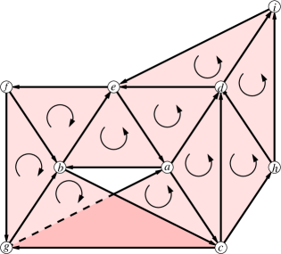
Figure 6: A $2$-complex illustrating an MNTUS and a CMNTUS. The Möbius strip formed by all triangles represents an MNTUS $M$ of the $2$-boundary matrix of the complex, but $M$ is not a CMNTUS. Edge $ad$ is the face of two triangles in this Möbius strip, and thus corresponds to an exterior row that has an even number of nonzeros in $Q_{M}$. The smaller Möbius strip formed by the seven triangles leaving out $die,dhi$, and $dch$ represents a CMNTUS $M^{\prime}$. Edge $ad$ is an interior row of $M^{\prime}$.

For any MNTUS $M$ of $[\partial_{q}]$ with $r$ rows, let $\mathscr{M}$ be the set of elements of $\operatorname{Ker}(A)$ whose nonzero $q$-coefficients are contained in $Q_{M}$. Because $\det(M)$ is nonzero, $\operatorname{Ker}(M)$ is trivial. This means there is a bijection between the set of linear combinations of columns of $M$, and the set of possible row sums of $M$. This, along with Lemma 3.5, implies that for any $\mathbf{m}^{1},\mathbf{m}^{2}\in\mathscr{M}$, the set of $p$-coefficients of interior rows of $\mathbf{m}^{1}$ and $\mathbf{m}^{2}$ are equal if and only if all $q$-coefficients of $\mathbf{m}^{1}$ and $\mathbf{m}^{2}$ are equal.

Definition 6.5.

For any row $i$ of $M$, let $[\mathbf{m}^{i}]$ denote the equivalence class of elements of $\mathscr{M}$ whose $p$-coefficients of interior rows is the unit vector with its nonzero coefficient at row $i$.

Letting $P_{M}$ represent the set of interior rows of $M$, another consequence of the kernel of $M$ being trivial, and the bijection between the set of linear combinations of columns of $M$ and the set of possible row sums of $M$, is that the following equation holds for any $\mathbf{m}\in\mathscr{M}$ with $p$-coefficients $\mathbf{p}$, and an appropriate choice of $\mathbf{m}^{i}$ from each $[\mathbf{m}^{i}]$.

$$\mathbf{m}=\sum_{i\in P_{M}}p_{i}\mathbf{m}^{i}.$$ (4)

The following lemma characterizes the fractional elements of $[\mathbf{m}^{i}]$ for any interior row $i$ of $M$.

Lemma 6.6.

For any MNTU submatrix $M$ of $[\partial_{q}]$, and any interior row $i$ of $M$, each $q$-coefficient of any element of $[\mathbf{m}^{i}]$ is nonzero if and only if it corresponds to a column of $Q_{M}$, and each such coefficient is $\pm(1/2)$.

Proof.

For an MNTUS $M$ of $[\partial_{q}]$, let $i$ be an interior row. Because $\det(M)\neq 0$, there is some entry $M_{ij}$ that is nonzero. If we multiply $M_{ij}$ by $-1$, and call the result $M^{\prime}$, then $M^{\prime}$ is Eulerian, and the sum of its entries is $0\bmod 4$. Therefore $M^{\prime}$ is totally unimodular. Hence there is some set $\mathscr{J}$ of columns of $M^{\prime}$ that we may multiply by $-1$, and if we call the result $M_{-\mathscr{J}}^{\prime}$, the sum of each row of $M_{-\mathscr{J}}^{\prime}$ must be $0,1$, or $-1$. Because $M_{-\mathscr{J}}^{\prime}$ is also Eulerian, each of these row sums must be $0$. If we now multiply $M_{ij}$ by $-1$ again and call the result $M_{-\mathscr{J}}$, the row sum of $i$ is $\pm 2$, and every other row sum is still 0. If the row sum of $i$ is $-2$, multiply all columns of $M_{-\mathscr{J}}$ by $-1$. Now call this result, whether this final inversion is necessary or not, $M_{i}$. The row sum for $i$ is 2, and all other row sums are 0, and $M_{i}$ is $M$ with some (perhaps empty) set of columns of $M$ scaled by $-1$. Therefore by Lemma 3.5 and equation (4), any element of $\mathscr{M}$ whose nonzero $q$-coefficients agree with the scalings of $M_{i}$ is twice some $\mathbf{m}^{i}\in[\mathbf{m}^{i}]$, and all these coefficients are either 1 or $-1$. Since any elements of $\mathscr{M}$ are equal in all $q$-coefficients if and only if they are equivalent, any $\mathbf{m}^{i}\in[\mathbf{m}^{i}]$ must have all nonzero $q$-coefficients be $\pm(1/2)$. ∎

From this result, the following Lemma is almost immediate, and its proof is omitted.

Lemma 6.7.

For a given MNTUS $M$, and any list of interior rows $i_{1},i_{2},...i_{n}$, and elements $\mathbf{m}^{i_{1}},\mathbf{m}^{i_{2}},...\mathbf{m}^{i_{n}}$ of $[\mathbf{m}^{i_{1}}],[\mathbf{m}^{i_{2}}],...[\mathbf{m}^{i_{n}}]$, respectively:

1. If $n=2$, all $q$-coefficients of both $\mathbf{m}^{i_{1}}+\mathbf{m}^{i_{2}}$ and $\mathbf{m}^{i_{1}}-\mathbf{m}^{i_{2}}$ are in $\{0,\pm 1\}$.

2. If $n=2$, for any $j\in Q_{M}$, the $j{\text{th}}\ q$-coefficient of $\mathbf{m}^{i_{1}}+\mathbf{m}^{i_{2}}$ is zero if and only if the $j{\text{th}}\ q$-coefficient of $\mathbf{m}^{i_{1}}-\mathbf{m}^{i_{2}}$ is nonzero.

3. If $n$ is even, $\sum_{\alpha=1,...n}\mathbf{m}^{i_{\alpha}}$ is integral.

4. If $n$ is odd, every nonzero $q$-coefficient of $\sum_{\alpha=1,...n}\mathbf{m}^{i_{\alpha}}$ is nonintegral, with each of these nonzero $q$-coefficients of the form $\frac{k}{2}$ with $k$ an odd integer

Note that nowhere in Lemma 6.7 is it required that $i_{\alpha}\neq i_{\beta}$ for any $\alpha,\beta,\in 1,2,...n$.

Definition 6.8.

For any MNTUS $M$ of $[\partial_{q}]$, and any concise $\mathbf{z}$, let $\mathbf{m}(\mathbf{z})$ be the unique element of $\mathscr{M}$ where $\{\mathbf{z},\mathbf{m}(\mathbf{z})\}$ is linearly concise, $z_{j}=0$ implies the $j{\text{th}}$ entry of $\mathbf{m}(\mathbf{z})$ is $\leq 0$ $~{}\forall j\leq 2(m+n)$, and for each interior row $i$ of $M$, the $i{\text{th}}\ p$-coefficient of $\mathbf{z}$ and $\mathbf{m}(\mathbf{z})$ are equal.

Equation 4 then restricts $\mathbf{m}(\mathbf{z})$ to a single equivalence class. The requirement to be linearly concise with $\mathbf{z}$ fixes coefficients of $\mathbf{m}(\mathbf{z})$ corresponding to nonzero $p$- and $q$-coefficients of $\mathbf{z}$, and also requires $\mathbf{m}(\mathbf{z})$ to be concise. Finally, the requirement on zero entries of $\mathbf{z}$ fixes the remaining entries of $\mathbf{m}(\mathbf{z})$ by dictating, in the case where a $p$- or $q$-coefficient is nonzero in $\mathbf{m}(\mathbf{z})$ but zero in $\mathbf{z}$, which entry among each pair of corresponding opposite entries is nonzero, thus making $\mathbf{m}(\mathbf{z})$ unique.

Theorem 6.9.

For any MNTUS $M$ of $[\partial_{q}]$, and any interior row $i$, there is a unique vertex $\mathbf{z}^{i}$ of $P_{i}$ whose nonzero $q$-coefficients are contained in $Q_{M}$ and whose $p$-coefficients of interior rows are all 0. This vertex is $\mathbf{z}^{I}-\mathbf{m}(\mathbf{z}^{I})$ where $\mathbf{z}^{I}$ is the identity solution to OHCP_i. Furthermore, if $M$ is a CMNTUS of $[\partial_{q}]$, $\mathbf{z}^{i}$ is the only nonintegral vertex of $P_{i}$ whose nonzero $q$-coefficients are contained in $Q_{M}$.

Proof.

Let $\mathbf{z}^{i}=\mathbf{z}^{I}-\mathbf{m}(\mathbf{z}^{I})$. Then $\mathbf{z}^{i}$ is feasible, and all $p$-coefficients of interior rows of $\mathbf{z}^{i}$ are zero. Because $\operatorname{Ker}(M)$ is trivial, this is the only concise feasible solution whose nonzero $q$-coefficients are contained in $Q_{M}$, with the $p$-coefficients of interior rows all zero. To show $\mathbf{z}^{i}$ is a basic solution, we try to decompose $-\mathbf{m}(\mathbf{z}^{I})$ into $\mathbf{z}^{C}+\mathbf{z}^{D}$ satisfying the properties specified in Theorem 3.9. Because $\operatorname{Ker}(M)$ is trivial, there must be some $x$-coordinate that is nonzero in $\mathbf{z}^{I}+\mathbf{z}^{C}$, but zero in $\mathbf{z}^{i}$, implying this coordinate is also nonzero in $\mathbf{z}^{D}$. Therefore Property 7 in Theorem 3.9 cannot be satisfied, and so $\mathbf{z}^{i}$ is a basic solution of OHCP_i.

Now assume $M$ is a CMNTUS. Let $\mathbf{z}$ be a basic solution not equivalent to $\mathbf{z}^{i}$ whose nonzero $q$-coefficients are contained in $Q_{M}$. Then by Lemma 3.7, the $p$-coefficient for some exterior row $i_{0}$ is nonzero in $\mathbf{z}^{i}$ but zero in $\mathbf{z}$.

Since $M$ is a CMNTUS, by Theorem 6.4, $i_{0}$ has an odd number of nonzero entries in $Q_{M}$. Then Lemma 6.6 implies that an odd number of the $q$-coefficients for the columns with these nonzero entries must be integral in $\mathbf{z}$.

Decompose $\mathbf{z}$ into $\mathbf{z}^{I}+\mathbf{z}^{R}+\mathbf{z}^{Z}$, where $\mathbf{z}^{R}$ is the element of $\mathscr{M}$ whose nonzero $q$-coefficients are equal to the nonintegral $q$-coefficients of $\mathbf{z}$, and $\mathbf{z}^{Z}$ is the element of $\mathscr{M}$ whose nonzero $q$-coefficients are equal to the integral $q$-coefficients of $\mathbf{z}$. Then $\mathbf{z}^{R}$ and $\mathbf{z}^{Z}$ cannot both be $\mathbf{0}$. If $\mathbf{z}^{I}+\mathbf{z}^{R}$ is a basic solution, then by Cramer’s Rule, this implies there is a non-TU matrix contained in the columns with nonzero $q$-coefficients in $\mathbf{z}^{R}$, contradicting $M$ being a CMNTUS.

If $\mathbf{z}^{I}+\mathbf{z}^{R}$ is not a basic solution, then by Theorem 3.3, there is some nonzero $\mathbf{z}^{K}\in\operatorname{Ker}(A)$ where all $p$- and $q$-coefficients nonzero in $\mathbf{z}^{K}$ are also nonzero in $\mathbf{z}^{I}+\mathbf{z}^{R}$. Since $\mathbf{z}$ is a basic solution, $\mathbf{z}^{Z}$ must cancel one of these coefficients. And since no nonzero $q$-coefficients in $\mathbf{z}^{R}$ are nonzero in $\mathbf{z}^{Z}$, these canceled coefficients must all be $p$-coefficients. Since all $q$-coefficients of $\mathbf{z}^{Z}$ are integral, all $p$-coefficients of $\mathbf{z}^{Z}$ are also integral. Then by Lemma 3.10, there must be at least two nonzero integral $p$-coefficients in $\mathbf{z}^{I}+\mathbf{z}^{R}$, and so there must be at least one in $\mathbf{z}^{R}$. If we construct the input chain whose nonzero coefficients are the values of each of the integral $p$-coefficients of $\mathbf{z}^{R}$ multiplied by $-1$, then $\mathbf{z}^{R}$ added to the identity solution for the OHCP with this input chain must be a basic solution to this OHCP. Then by Lemma 4.3, there must be some OHCP_j where $\mathbf{z}^{R}$ added to the identity solution for OHCP_j is basic. Hence, again by Cramer’s Rule, there is a non-TU submatrix contained in the columns with nonzero $q$-coefficients in $\mathbf{z}^{R}$, contradicting $M$ being columnwise minimal. ∎

Remark 6.10.

The result in Theorem 6.9 holds for the case of $-\mathbf{e}_{i}$ as the elementary input chain (for OHCP_-i), instead of the standard case of $\mathbf{e}_{i}$. But in this case, the unique vertex, which we call $\mathbf{z}^{-i}$, will be distinct from $\mathbf{z}^{i}$ as used in the original statement of the Theorem. In further discussion, it is understood that when we refer to $\mathbf{z}^{i}$, we cover both these possibilities.

Lemma 6.11.

For a set of columns $Q$ of $[\partial_{q}]$, let there be no $i$ such that OHCP_i has a nonintegral basic solution in $\left(P_{A}\right)_{i}$ whose nonzero $q$-coefficients are contained in $Q$. Then for any basic solution $\mathbf{z}^{Y}$ of any $OHCP_{i}$ in $\left(P_{A}\right)_{i}$ whose nonzero $q$-coefficients are contained in $Q$, all $p$-coefficients of $\mathbf{z}^{Y}$ are in $\{0,\pm 1\}$.

Proof.

If $\mathbf{z}^{Y}$ is a basic solution in $\left(P_{A}\right)_{i}$ to OHCP_i for some $i$ whose nonzero $q$-coefficients are contained in $Q$, it must be integral. Let $\mathbf{z}^{K}=\mathbf{z}^{Y}-\mathbf{z}^{I}$, where $\mathbf{z}^{I}$ is the identity solution. If $\mathbf{z}^{Y}$ has a coefficient $\alpha$ for the $x$-coordinate $i_{0}$ where $\lvert\alpha\rvert>1$, then by Lemma 4.1 and Theorem 3.9, if we let $\mathbf{z}^{I_{0}}$ be the identity solution to the OHCP LP $O_{0}$ whose input chain has all zeros except for coordinate $i_{0}$, which has coefficient $\pm 1$ that is opposite in sign to the coefficient of $i_{0}$ in $\mathbf{z}^{Y}$, then $\mathbf{z}^{I_{0}}+\displaystyle\frac{1}{\alpha}\mathbf{z}^{K}$ is a basic solution to $O_{0}$ with the $p$-coefficient of $i$ being the nonintegral value $-(1/\alpha)$. However, any basic solution of $O_{0}$ where the nonzero $q$-coefficients are contained in $Q$ must still be integral, giving us a contradiction. ∎

7 NTU Neutralized Complexes

We define the concept of NTU neutralization, and present results characterizing this condition.

Definition 7.1.

For any interior row $i$ of an MNTUS $M$ of $[\partial_{q}]$, let $\mathbf{k}^{i}$ represent a concise integral element of $\operatorname{Ker}(A)$ whose sum of $p$-coefficients of interior rows is odd, $\left(\mathbf{k}^{i}-\mathbf{m}(\mathbf{k}^{i})\right)\arrowvert_{\mathscr{X}}\neq\mathbf{0}$, and let the absolute value of each $p$-coefficient of $\mathbf{k}^{i}-\mathbf{m}(\mathbf{k}^{i})$ be less than or equal to the absolute value of this coefficient in $\mathbf{z}^{i}$. If each interior row $i$ of $M$ has such a $\mathbf{k}^{i}$, then $M$ is neutralized. If all MNTU submatrices of $[\partial_{q}]$ are neutralized, then $K$ is NTU neutralized in the $q{\text{th}}$ dimension.

Theorem 7.2.

For any MNTUS $M$ of $[\partial_{q}]$, the projection $\mathbf{z}^{i}\arrowvert_{\mathscr{X}}$ for each interior row $i$ is a convex combination of $\mathbf{z}^{1}\arrowvert_{\mathscr{X}}$ and $\mathbf{z}^{2}\arrowvert_{\mathscr{X}}$ where both $\mathbf{z}^{1}$ and $\mathbf{z}^{2}$ are integral elements of $P_{i}$ if and only if $M$ is neutralized.

Proof.

First, we the ignore the restriction that $\mathbf{z}^{1}$ and $\mathbf{z}^{2}$ are integral, and say by Corollary 5.3 that each $\mathbf{z}^{i}\arrowvert_{\mathscr{X}}$ is not a basic solution to OHCP${}_{i}\arrowvert_{\mathscr{X}}$, and hence a convex combination of $\mathbf{z}^{1}\arrowvert_{\mathscr{X}}$ and $\mathbf{z}^{2}\arrowvert_{\mathscr{X}}$ with $\mathbf{z}^{1},\mathbf{z}^{2}\in P_{i}$, if and only if there exists a $\mathbf{k}_{\text{ex}}^{i}$ with $\mathbf{k}_{\text{ex}}^{i}\arrowvert_{\mathscr{X}}\neq\mathbf{0}$, and where all nonzero coefficients of $\mathbf{k}_{\text{ex}}^{i}\arrowvert_{\mathscr{X}}$ are nonzero in $\mathbf{z}^{i}$.

If for a given $\mathbf{z}^{i}$ there is a $\mathbf{k}^{i}$ satisfying Definition 7.1, by Lemma 3.11 we may adjust $\mathbf{k}^{i}$ and $\mathbf{m}(\mathbf{k}^{i})$ if necessary so that $\{\mathbf{k}^{i},\mathbf{z}^{i},\mathbf{m}(\mathbf{k}^{i})\}$ is linearly concise. Then $\mathbf{k}^{i}-\mathbf{m}(\mathbf{k}^{i})$ satisfies the conditions for $\mathbf{k}_{\text{ex}}^{i}$. So let $\mathbf{k}_{\text{ex}}^{i}=\mathbf{k}^{i}-\mathbf{m}(\mathbf{k}^{i})$. Since $\mathbf{k}^{i}$ is integral, by Lemma 6.7, each $q$-coefficient in $Q_{M}$ of $\mathbf{k}_{\text{ex}}^{i}$ is nonintegral with a denominator 2. By Lemma 6.6 and Theorem 6.9, this is also true of $\mathbf{z}^{i}$. Every other $q$-coefficient in both $\mathbf{k}_{\text{ex}}^{i}$ and $\mathbf{z}^{i}$ is integral. Hence if we let $\mathbf{z}^{1}=\mathbf{z}^{i}+\mathbf{k}_{\text{ex}}^{i}$, and $\mathbf{z}^{2}=\mathbf{z}^{i}-\mathbf{k}_{\text{ex}}^{i}$, then both $\mathbf{z}^{1}$ and $\mathbf{z}^{2}$ are integral. Because the absolute value of each $p$-coefficient of $\mathbf{k}_{\text{ex}}^{i}$ is less than or equal to the absolute of this coefficient in $\mathbf{z}^{i}$, $\mathbf{z}^{1}\arrowvert_{\mathscr{X}}$ and $\mathbf{z}^{2}\arrowvert_{\mathscr{X}}$ are both in $P_{i}\arrowvert_{\mathscr{X}}$. If either $\mathbf{z}^{1}$ or $\mathbf{z}^{2}$ is not in $P_{i}$, then by Corollary 3.14 we may use the same method as in Corollary 3.13 to transform either into some solution that is concise, integral, feasible, equivalent, and with all $x$-coefficients unchanged, keeping $\mathbf{z}^{i}\arrowvert_{\mathscr{X}}$ a convex combination of $\mathbf{z}^{1}\arrowvert_{\mathscr{X}}$ and $\mathbf{z}^{2}\arrowvert_{\mathscr{X}}$.

Now suppose that for some $i$, $\mathbf{z}^{i}\arrowvert_{\mathscr{X}}$ is a convex combination of $\mathbf{z}^{1}\arrowvert_{\mathscr{X}}$ and $\mathbf{z}^{2}\arrowvert_{\mathscr{X}}$ with $\mathbf{z}^{1}$ and $\mathbf{z}^{2}$ feasible and integral. Then there must be some $\mathbf{k}_{\text{ex}}^{i}$ satisfying the same qualities as above, and some $\alpha>0$ and $\beta<0$ where $\mathbf{z}^{i}+\alpha\mathbf{k}_{\text{ex}}^{i}$ and $\mathbf{z}^{i}+\beta\mathbf{k}_{\text{ex}}^{i}$ are both integral with their projections in $P_{i}\arrowvert_{\mathscr{X}}$.

Let $\alpha$ be of least absolute value such that $\mathbf{z}^{i}+\alpha\mathbf{k}_{\text{ex}}^{i}$ is integral. Because both $(\mathbf{z}^{i}+\alpha\mathbf{k}_{\text{ex}}^{i})\arrowvert_{\mathscr{X}}$ and $(\mathbf{z}^{i}-\alpha\mathbf{k}_{\text{ex}}^{i})\arrowvert_{\mathscr{X}}$ are in $P_{i}\arrowvert_{\mathscr{X}}$, the absolute value of each $p$-coefficient of $\alpha\mathbf{k}_{\text{ex}}^{i}$ is less than the absolute value of this coefficient in $\mathbf{z}^{i}$.

All $q$-coefficients of $\alpha\mathbf{k}_{\text{ex}}^{i}$ in $Q_{M}$ must be nonintegral with denominator 2, and all other $q$-coefficients integral. Hence for any interior row $j$, there is some $\mathbf{m}^{j}\in[\mathbf{m}^{j}]$ where $\alpha\mathbf{k}_{\text{ex}}^{i}+\mathbf{m}^{j}$ is concise and integral. Then any such $\alpha\mathbf{k}_{\text{ex}}^{i}+\mathbf{m}^{j}$ satisfies the conditions for $\mathbf{k}^{i}$. ∎

We now present out main result, which states that the complex being NTU neutralized is equivalent to none of the nonintegral vertices of the OHCP LP projecting down to vertices in the projection $P\arrowvert_{\mathscr{X}}$. Hence we cannot have a unique fractional optimal solution when the complex is NTU neutralized.

Theorem 7.3.

For a given complex $K$ with boundary matrix $[\partial_{q}]$, the projection $\mathbf{z}\arrowvert_{\mathscr{X}}$ of each nonintegral vertex $\mathbf{z}$ of any OHCP LP over $K$ with integral input $p$-chain $\mathbf{c}$ and polyhedron $P$ is not a vertex of $P\arrowvert_{\mathscr{X}}$ if and only if $K$ is NTU neutralized in the $q{\text{th}}$ dimension.

Proof.

First, we show that $K$ being neutralized is a necessary condition. If $K$ is not neutralized, then by Theorem 7.2, for some $i$ and MNTU $M$, there is a $\mathbf{z}^{i}$ where $\mathbf{z}^{i}\arrowvert_{\mathscr{X}}$ is not a convex combination of $\mathbf{z}^{1}\arrowvert_{\mathscr{X}}$ and $\mathbf{z}^{2}\arrowvert_{\mathscr{X}}$ with both $\mathbf{z}^{1}$ and $\mathbf{z}^{2}$ integral elements of $P_{i}$. If $\mathbf{z}^{i}\arrowvert_{\mathscr{X}}$ is not a convex combination of any two points in $P_{i}\arrowvert_{\mathscr{X}}$, then it is a vertex of $P_{i}\arrowvert_{\mathscr{X}}$.

If $\mathbf{z}^{i}\arrowvert_{\mathscr{X}}$ is a convex combination of $\mathbf{z}^{1}\arrowvert_{\mathscr{X}}$ and $\mathbf{z}^{2}\arrowvert_{\mathscr{X}}$, then by Corollary 5.3, and taking the notation from Theorem 7.2, there is some $\mathbf{k}_{\text{ex}}^{i}$ and some rational number $\alpha>0$ such that $\left(\mathbf{z}^{i}\pm\alpha\mathbf{k}_{\text{ex}}^{i}\right)\arrowvert_{\mathscr{X}}$ is in $P_{i}\arrowvert_{\mathscr{X}}$. Since all variables of OHCP_i are bounded, there exists a largest value of $\alpha$ for which this is true. Let $\alpha$ have this largest possible value. Then either $\left(\mathbf{z}^{i}+\alpha\mathbf{k}_{\text{ex}}^{i}\right)\arrowvert_{\mathscr{X}}$ or $\left(\mathbf{z}^{i}-\alpha\mathbf{k}_{\text{ex}}^{i}\right)\arrowvert_{\mathscr{X}}$ brings one of the nonzero coefficients of $\mathbf{k}_{\text{ex}}^{i}\arrowvert_{\mathscr{X}}$ to $0$. Suppose without loss of generality that this condition is true for $\left(\mathbf{z}^{i}+\alpha\mathbf{k}_{\text{ex}}^{i}\right)\arrowvert_{\mathscr{X}}$. If $\left(\mathbf{z}^{i}+\alpha\mathbf{k}_{\text{ex}}^{i}\right)\arrowvert_{\mathscr{X}}$ is not a basic solution of (OHCP${}_{i})\arrowvert_{\mathscr{X}}$, this means there is some other $\mathbf{k}_{\text{ex}}^{i\prime}$, with some other $\alpha^{\prime}$. In this case, let $\alpha\mathbf{k}_{\text{ex}}^{i}$ represent the sum of each such $\alpha\mathbf{k}_{\text{ex}}^{i}$, making $\left(\mathbf{z}^{i}+\alpha\mathbf{k}_{\text{ex}}^{i}\right)\arrowvert_{\mathscr{X}}$ a basic solution.

If $\mathbf{z}^{i}+\alpha\mathbf{k}_{\text{ex}}^{i}$ is not integral, then by Corollary 5.12, and Lemma 5.6, there is some corresponding vertex $\mathbf{z}^{1}$ of OHCP_i that is nonintegral, and $\mathbf{z}^{1}\arrowvert_{\mathscr{X}}$ is a vertex of $P_{i}\arrowvert_{\mathscr{X}}$. If $\mathbf{z}^{i}+\alpha\mathbf{k}_{\text{ex}}^{i}$ is integral, let $\beta$ be a nonzero rational value opposite in sign to $\alpha$. There must be some such $\beta$ where $\left(\mathbf{z}^{i}+\beta\mathbf{k}_{\text{ex}}^{i}\right)\arrowvert_{\mathscr{X}}$ is in $P_{i}\arrowvert_{\mathscr{X}}$. If there is a maximum absolute value for such a $\beta$, then because $\mathbf{z}^{i}\arrowvert_{\mathscr{X}}$ is not a convex combination of $\mathbf{z}^{1}\arrowvert_{\mathscr{X}}$ and $\mathbf{z}^{2}\arrowvert_{\mathscr{X}}$, with both $\mathbf{z}^{1}$ and $\mathbf{z}^{2}$ integral, $\mathbf{z}^{i}+\beta\mathbf{k}_{\text{ex}}^{i}$ is nonintegral, and by a similar logic as the $\alpha$ case, there is some $\mathbf{z}^{2}$ of OHCP_i that is nonintegral, and $\mathbf{z}^{2}\arrowvert_{\mathscr{X}}$ is a vertex of $P_{i}\arrowvert_{\mathscr{X}}$.

If $\mathbf{z}^{i}+\alpha\mathbf{k}_{\text{ex}}^{i}$ is integral, then if there is no upper bound for the absolute value of $\beta$, because $\operatorname{Ker}(A)$ is rational, there must be some $\mathbf{z}^{i}+\beta\mathbf{k}_{\text{ex}}^{i}$ that is integral, contradicting $\mathbf{z}^{i}\arrowvert_{\mathscr{X}}$ not being a convex combination of $\mathbf{z}^{1}\arrowvert_{\mathscr{X}}$ and $\mathbf{z}^{2}\arrowvert_{\mathscr{X}}$, with both $\mathbf{z}^{1}$ and $\mathbf{z}^{2}$ integral. Therefore $K$ being NTU neutralized in the $q{\text{th}}$ dimension is necessary for the projection $\mathbf{z}\arrowvert_{\mathscr{X}}$ of each nonintegral vertex $\mathbf{z}$ of any OHCP LP over $K$ with integral input $p$-chain $\mathbf{c}$ and polyhedron $P$ to not be a vertex of $P\arrowvert_{\mathscr{X}}$.

Now assume all MNTUS of $[\partial_{q}]$ are neutralized. Suppose for some OHCP LP, there is a nonintegral vertex $\mathbf{z}$ where $\mathbf{z}\arrowvert_{\mathscr{X}}$ is a vertex of $P\arrowvert_{\mathscr{X}}$. Then by Theorem 5.14, for some $i$, there is a nonintegral $\mathbf{z}^{\prime}$ where $\mathbf{z}^{\prime}\arrowvert_{\mathscr{X}}$ is a vertex of $P_{i}\arrowvert_{\mathscr{X}}$, and Corollary 5.15 implies that there is such a $\mathbf{z}^{\prime}$ where all nonzero $q$-coefficients are nonintegral. We will attempt to find a minimal set $Q$ of columns of $[\partial_{q}]$ that contains the nonzero $q$-coefficients of such a $\mathbf{z}^{\prime}$.

By Cramer’s Rule, and the definition of columnwise minimality, $Q$ must contain the columns of a CMNTUS $M$ where $i$ is an interior row of $M$. But we know from Theorem 7.2 this is not enough because of some $\mathbf{k}^{i}$ with $\mathbf{z}^{\prime}\pm\left(\mathbf{k}^{i}-\mathbf{m}(\mathbf{k}^{i})\right)$ integral.

By Corollary 5.10, we must add $q$-simplices until there exist $p$-coefficients $r$ and $s$ as in Lemma 3.10. Hence $r$ and $s$ are exterior rows of $M$. Further, $r$, $s$, and $i$ are interior rows of some orientation-reversing $q$-chain $C$.

By Lemma 6.11, all newly added $q$-coefficients, and therefore all $q$-coefficients of $C$, are the same in absolute value. So if the columns of $C$ contain an MNTUS, the $q$-coefficients of the simplices in $C$ is a solution of the form $\mathbf{z}^{i}$ (see Remark 6.10). Therefore Theorem 7.2 applies and we have another $\mathbf{z}^{i}\pm\left(\mathbf{k}^{i}-\mathbf{m}(\mathbf{k}^{i})\right)$ that is integral. Any solution basic in OHCP_i must be some combination of this $\mathbf{z}^{i}$ and the previous $\mathbf{z}^{\prime}$, and so the projection of any such basic solution must be a convex combination of at least two projections of these four integral values.

If the columns of $C$ do not contain an MNTUS, then by Cramer’s Rule, no nonintegral vertices can be added.

So we still have not found any vertex of $P_{i}$ whose projection is a vertex of $P_{i}\arrowvert_{\mathscr{X}}$. But each time we add $q$-coefficients in a minimal way to find such a vertex, we may repeat the same logic as above. Therefore no such vertex can exist. ∎

Remark 7.4.

In either the left or right triangulation of the Example in Section 1.1 for the OHCP with input chain $ef$, $\mathbf{z}^{i}\arrowvert_{\mathscr{X}}$ is all black solid edges, each with a coefficient of $0.5$ (see Figure 1). $\mathbf{m}(\mathbf{z}^{I})\arrowvert_{\mathscr{X}}$ is the union of these black solid edges, each with coefficient $-0.5$, together with edge $ef$ with coefficient $1$. In the right triangulation, the light and dark gray chains are projections of two integral vertices $\mathbf{z}^{1}\arrowvert_{\mathscr{X}}$ and $\mathbf{z}^{2}\arrowvert_{\mathscr{X}}$, respectively. All coefficients in both of these projections are 1. Triangle $adc$ satisfies all criteria for $\mathbf{k}^{i}$. Then $\mathbf{z}^{i}\arrowvert_{\mathscr{X}}=(1/2)(\mathbf{z}^{1}\arrowvert_{\mathscr{X}}+\mathbf{z}^{2}\arrowvert_{\mathscr{X}})$. Also, $\mathbf{m}(\mathbf{k}^{i})\arrowvert_{\mathscr{X}}=\mathbf{k}^{i}\arrowvert_{\mathscr{X}}-(1/2)(\mathbf{z}^{1}\arrowvert_{\mathscr{X}}-\mathbf{z}^{2}\arrowvert_{\mathscr{X}})$, and $\mathbf{z}^{1}\arrowvert_{\mathscr{X}}-(\mathbf{k}^{i}-\mathbf{m}(\mathbf{k}^{i}))\arrowvert_{\mathscr{X}}=\mathbf{z}^{2}\arrowvert_{\mathscr{X}}+(\mathbf{k}^{i}-\mathbf{m}(\mathbf{k}^{i}))\arrowvert_{\mathscr{X}}=\mathbf{z}^{i}\arrowvert_{\mathscr{X}}$.

7.1 Connections to integral polytopes and TDI systems

There exist conditions weaker than the constraint matrix being TU, which still guarantee that the LP has integral optimal solutions in certain cases [21, Chap. 21,22]. In particular, $k$-balanced matrices define a hierarchy of such matrices, with TU matrices at one end [7]. The matrix $A$ is $k$-balanced for any $k\in{\mathbb{Z}}_{>0}$ if $A_{ij}\in\{0,\pm 1\}$ and $A$ does not contain an MNTUS with at most $2k$ nonzero entries in each row. If the constraint matrix $A$ of the IP in Equation (1) is $k$-balanced, then for certain integral right-hand sides $\mathbf{b}$, the polytope of the associated LP is integral [7]. At the same time, the polytope of the OHCP LP is not integral even when the simplicial complex is NTU neutralized. Indeed, the constraint matrix $A$ in not $k$-balanced for any $k$ in this case.

A linear system $A^{T}\mathbf{y}\leq\mathbf{f}$ is totally dual integral (TDI) if the LP $~{}\min\,\{\mathbf{f}^{T}\mathbf{x}~{}|~{}A\mathbf{x}=\mathbf{c},\;\mathbf{x}\geq\mathbf{0}\}~{}$ has an integral optimal solution for every $\mathbf{c}\in{\mathbb{Z}}^{m}$ for which the minimum is finite. Every OHCP instance has a finite minimum, and when the complex is NTU neutralized, the OHCP LP is guaranteed to have an integral optimal solution. Hence the linear system $A^{T}\mathbf{y}\leq\mathbf{f}$ defined by the dual of the OHCP LP (3) using $\mathbf{f}^{T}=\begin{bmatrix}\mathbf{w}^{T}&\mathbf{w}^{T}&\mathbf{0}^{T}&\mathbf{0}^{T}\end{bmatrix}$ is TDI. This correspondence sheds some light on the complexity of checking if a given complex is NTU neutralized. The problem of checking if a linear system is TDI is coNP-complete [13], but could be done in polynomial time if the dimension, or equivalently, $\operatorname{rank}(A)$ is fixed [9, 20].

8 A Class of NTU Neutralized Complexes

In this section, we identify a class of complexes that may have relative torsion, but are guaranteed to be NTU Neutralized. This is the class of $2$-complexes whose first homology group is trivial.

Theorem 8.1.

If a $2$-complex has the trivial first homology group (over ${\mathbb{Z}}$), then it is NTU-neutralized.

Proof.

Any MNTU in $[\partial_{2}]$ is a Möbius strip $M$ where each interior edge is the face of exactly two triangles of $M$. First, let us assume each exterior edge is the face of exactly one triangle of $M$. Then for any $\mathbf{z}^{i}$, if we think of the elementary input edge as a path from its end points $v_{1}$ and $v_{2}$, this fractional vertex splits this path evenly into two distinct simple paths that together traverse all exterior edges of $M$. Consider the direction of both these fractional paths as positive, so that each edge in $\mathbf{z}^{i}$ has a coefficient of $+1/2$ under this consideration.

Now consider the general case where exterior edges may be the face of more than one triangle in $M$. The two fractional paths may not be simple now, and may loop back on themselves or each other. Some of the resulting coefficients of exterior edges may now cancel each other out, and may even become negative. But because these paths are simple and distinct in the previous case, with all coefficients of $+1/2$, the exterior edges still must contain a path from $v_{1}$ to $v_{2}$ whose coefficients are all at least $+1/2$. Call this path $h$.

In the actual complex, the coefficients of $h$ in $\mathbf{z}^{i}$ may be positive or negative. But they will have the same absolute value as our construction above. Adding a path $h^{\prime}$ of coefficient 1 in the opposite direction from $v_{2}$ to $v_{1}$ along $h$ is equivalent to adding $-1$ to each of the strictly positive coefficients. Therefore because each of the strictly positive coefficients were at least $+1/2$, adding this path from $v_{2}$ to $v_{1}$ will not increase the absolute value of any coefficients in $h$, or in fact for any coefficients in $\mathbf{z}^{i}$. The path $h^{\prime}$, together with the elementary input edge, forms a loop $l$.

Since the 1-homology of the complex is trivial, $l$ must be null-homologous, and so is equivalent to the $x$-coefficients of some integral element $\mathbf{k}^{i}$ of $\operatorname{Ker}(A)$. The sum of coefficients of interior edges in $\mathbf{k}^{i}$ is odd, and $\mathbf{m}(\mathbf{k}^{i})=\mathbf{m}(\mathbf{z}^{I})$. Since $\mathbf{k}^{i}\arrowvert_{\mathscr{X}}=\mathbf{z}^{I}+h^{\prime}$, and by the properties of $h^{\prime}$ relative to $\mathbf{z}^{i}$ described above, the absolute value of each 1-coefficient of $\mathbf{k}^{i}-\mathbf{m}(\mathbf{k}^{i})$ is less than or equal to the absolute value of this coefficient in $\mathbf{z}^{i}$. Therefore $\mathbf{z}^{i}$ is neutralized, and since it is arbitrary, the complex is NTU Neutralized. ∎

Remark 8.2.

In Figure 1, the left complex becomes a member of the subclass described in Theorem 8.1 if we add the triangles $akm$ and $dfh$. As mentioned earlier, adding triangle $akm$ alone is enough to make the complex NTU neutralized, though.

Remark 8.3.

For a $2$-complex, we could check more efficiently whether the first homology group is trivial [14] than checking whether the boundary matrix is TU [22]. If the former condition holds, then we can be sure that all OHCP instances on this complex can be solved efficiently.

9 Discussion

Our results on MNTUS, in particular from Section 6, are specifically for such submatrices of the boundary matrices of simplicial complexes. NTU neutralized complexes define a class of LPs with unique structure – these OHCP LP polytopes may not be integral, yet, for every input chain, i.e., for every integral right-hand side, there exists an integral optimal solution. Our main result (Theorem 7.3) implies that when $K$ is NTU neutralized, if an optimal solution of the OHCP LP is nonintegral then there must exist another integral optimal solution with the same total weight. If a standard LP algorithm finds the fractional optimal solution, we should be able to find an adjacent integral optimal solution using an approach similar to that of Güler et al. [18] for the same task in the context of interior point methods for linear programming. This approach should run in strongly polynomial time.

While checking whether a linear system is TDI is coNP-complete, it is not known whether a direct polynomial time approach could be devised to check if the simplicial complex is NTU neutralized. Another interesting question is whether the definition of the complex being NTU neutralized could be simplified for low dimensional cases, which could also be tested efficiently. We identify one class of simplicial complexes that are guaranteed to be NTU neutralized (Section 8). Are there other special classes of complexes that are guaranteed to be NTU neutralized? The NTU neutralized complex (in right) in Figure 1 illustrates a case where the same neutralizing chain neutralizes all relevant elementary chains. A characterization of the structure of such complexes could also prove very useful.

References

- [1] Paul Camion. Characterization of Totally Unimodular Matrices. Proceedings of the American Mathematical Society, 16(5):1068–1073, 1965.
- [2] Erin W. Chambers, Éric Colin de Verdière, Jeff Erickson, Francis Lazarus, and Kim Whittlesey. Splitting (complicated) surfaces is hard. Comput. Geom. Theory Appl., 41:94–110, 2008.
- [3] Erin W. Chambers, Jeff Erickson, and Amir Nayyeri. Minimum cuts and shortest homologous cycles. In SCG ’09: Proc. 25th Ann. Sympos. Comput. Geom., pages 377–385, 2009.
- [4] Chao Chen and Daniel Freedman. Hardness results for homology localization. In SODA ’10: Proc. 21st Ann. ACM-SIAM Sympos. Discrete Algorithms, pages 1594–1604, 2010.
- [5] Chao Chen and Daniel Freedman. Measuring and computing natural generators for homology groups. Computational Geometry, 43(2):169–181, 2010. Special Issue on the 24th European Workshop on Computational Geometry (EuroCG’08).
- [6] Michele Conforti, Gérard Cornuéjols, and Klaus Truemper. From Totally Unimodular to Balanced Matrices: A Family of Integer Polytopes. Mathematics of Operations Research, 19(1):21–23, 1994.
- [7] Michele Conforti, Gérard Cornuéjols, and Kristina Vušković. Balanced matrices. Discrete Mathematics, 306(19–20):2411 – 2437, 2006.
- [8] Michele Conforti and Mendu R. Rao. Structural properties and recognition of restricted and strongly unimodular matrices. Mathematical Programming, 38:17–27, 1987.
- [9] William Cook, Laszlo Lovász, and Alexander Schrijver. A polynomial-time test for total dual integrality in fixed dimension. In Bernhard Korte and Klaus Ritter, editors, Mathematical Programming at Oberwolfach II, volume 22 of Mathematical Programming Studies, pages 64–69. Springer Berlin Heidelberg, 1984.
- [10] Vin de Silva and Robert Ghrist. Homological sensor networks. Notices of the American Mathematical Society, 54(1):10–17, 2007.
- [11] Tamal K. Dey, Anil N. Hirani, and Bala Krishnamoorthy. Optimal homologous cycles, total unimodularity, and linear programming. SIAM Journal on Computing, 40(4):1026–1040, 2011. arxiv:1001.0338.
- [12] Tamal K. Dey, Kuiyu Li, Jian Sun, and David Cohen-Steiner. Computing geometry-aware handle and tunnel loops in 3d models. In SIGGRAPH ’08: ACM SIGGRAPH 2008 papers, pages 1–9, New York, NY, USA, 2008.
- [13] Guoli Ding, Li Feng, and Wenan Zang. The complexity of recognizing linear systems with certain integrality properties. Mathematical Programming, 114(2):321–334, 2008.
- [14] Jean-Guillaume Dumas, Frank Heckenbach, David Saunders, and Volkmar Welker. Computing simplicial homology based on efficient smith normal form algorithms. In Michael Joswig and Nobuki Takayama, editors, Algebra, Geometry and Software Systems, pages 177–206. Springer Berlin Heidelberg, 2003.
- [15] Nathan M. Dunfield and Anil N. Hirani. The least spanning area of a knot and the optimal bounding chain problem. In Prooceedings of the 27th ACM Annual Symposium on Computational Geometry, SoCG ’11, pages 135–144, 2011.
- [16] Herbert Edelsbrunner, David Letscher, and Afra Zomorodian. Topological persistence and simplification. Discrete Comput. Geom., 28:511–533, 2002.
- [17] Éric Colin de Verdière and Jeff Erickson. Tightening non-simple paths and cycles on surfaces. In SODA ’06: Proc. 17th Ann. ACM-SIAM Sympos. Discrete Algorithms, pages 192–201, 2006.
- [18] Osman Güler, Dick den Hertog, Cornelis Roos, Tamas Terlaky, and Takashi Tsuchiya. Degeneracy in interior point methods for linear programming: a survey. Annals of Operations Research, 46-47(1):107–138, March 1993.
- [19] James R. Munkres. Elements of Algebraic Topology. Addison–Wesley Publishing Company, Menlo Park, 1984.
- [20] Edwin O’Shea and András Sebö. Alternatives for testing total dual integrality. Mathematical Programming, 132(1-2):57–78, 2012.
- [21] Alexander Schrijver. Theory of Linear and Integer Programming. Wiley-Interscience Series in Discrete Mathematics. John Wiley & Sons Ltd., Chichester, 1986.
- [22] Paul D. Seymour. Decomposition of regular matroids. J. Combin. Theory Ser. B, 28(3):305–359, 1980.
- [23] Alireza Tahbaz-Salehi and Ali Jadbabaie. Distributed coverage verification algorithms in sensor networks without location information. IEEE Transactions on Automatic Control, 55(8):1837–1849, 2010.
- [24] Klaus Truemper. A decomposition theory for matroids. VII. analysis of minimal violation matrices. Journal of Combinatorial Theory, Series B, 55(2):302–335, 1992.