Wide-field wide-band interferometric imaging: The WB A-Projection and hybrid algorithms

Abstract

Variations of the antenna primary beam (PB) pattern as a function of time, frequency and polarization form one of the dominant direction-dependent effects at most radio frequency bands. These gains may also vary from antenna to antenna. The A-Projection algorithm, published earlier, accounts for the effects of the narrow-band antenna PB in full polarization. In this paper we present the Wide-Band A-Projection algorithm (WB A-Projection) to include the effects of wide bandwidth in the A-term itself and show that the resulting algorithm simultaneously corrects for the time, frequency and polarization dependence of the PB. We discuss the combination of the WB A-Projection and the Multi-term Multi Frequency Synthesis (MT-MFS) algorithm for simultaneous mapping of the sky brightness distribution and the spectral index distribution across a wide field of view. We also discuss the use of the narrow-band A-Projection algorithm in hybrid imaging schemes that account for the frequency dependence of the PB in the image domain.

1. Introduction

Observations in the radio band offer distinct, and often times unique, scientific advantages in probing certain areas of astrophysical research (e.g in the detection of the EoR signal, studies of the high-redshift universe in general, large-scale structure formation, early galaxies, etc.).

All next generation radio telescopes, many in operation now, offer at least an order of magnitude improvement in the sensitivity and angular resolution compared to the telescopes operated in the past decades. The two key instrumental parameters which afford such high sensitivities, impact the imaging performance and are significantly different from previous generation telescopes are: 1) the wide instantaneous fractional bandwidths, and 2) larger collecting area. The effects of wide instantaneous fractional bandwidths that classical calibration and imaging algorithms ignore, lead to errors higher than the sensitivity that these new telescopes offer. Examples, relevant for some of the telescopes already in operation include the effects of time and frequency variant primary beams, frequency dependence of the emission from the sky and antenna pointing errors. The effects of wide fractional bandwidth and ionospheric phase screen limit the imaging performance below $\sim$1GHz. Additionally, significant variations in the shape of the wide-band primary beams (PB) for aperture array telescopes leads to errors of similar magnitude. All these effects form the general class of problems referred to in the literature as “direction dependent effects” or DD effects.

Both, wide fractional bandwidths and larger collecting area lead to many orders of magnitude increase in the data volume, putting severe constraints on the run-time performance of the algorithms for calibration and imaging. Furthermore, the cost of software development and maintenance also scales with algorithm complexity. Efficient algorithms to simultaneously account for all time-, frequency- and polarization-dependent DD effects which can also process large data volumes without significantly increasing algorithmic and software complexity are required.

In the following sections we discuss various possible approaches to full-beam wide-band continuum imaging. We present a modification of the A-Projection algorithm which we call the Wide-band A-Projection, or WB A-Projection algorithm where a modified A-term also compensates, to a large extent, the frequency dependence of the PB. We also discuss the use of the unmodified A-Projection algorithm (Bhatnagar et al. 2008, henceforth referred to as Paper-I), which we call the Narrow-band A-Projection, or NB A-Projection, along with various forms of image-plane normalizations for wide-band continuum imaging and the resulting issues and limitations.

2. Theory

Using the notation developed by Hamaker et al. (1996), full polarimetric measurements from a single baseline calibrated for the effects of direction-independent gains, can be described by the following Measurement Equation

$$\vec{V}^{Obs}_{ij}(\nu,t)=W_{ij}(\nu,t)\int P^{Sky}_{ij}(\vec{s},\nu,t)\vec{I}(\vec{s},\nu)e^{\iota\vec{b}_{ij}\cdot\vec{s}}d\vec{s}$$ (1)

where $\vec{V}^{Obs}_{ij}$ are the observed visibility samples measured by the pair of antennas designated by the subscript $i$ and $j$, separated by the vector $\vec{b}_{ij}$ and weighted by the measurement weights $W_{ij}$. $P^{Sky}_{ij}$ is the radio-Muëller matrix in the image domain representing the full polarization description of the antenna primary beams as a function of the direction $\vec{s}$, frequency $\nu$ and time $t$ and $\vec{I}$ is the image vector. The vectors $\vec{V}$ and $\vec{I}$ are full polarization vectors in the data and image domain respectively. $P^{Sky}_{ij}$ and $\vec{I}$ are the unknowns in this equation.

Equation 1 cannot be directly inverted as, in general, it is not a Fourier transform relation. It is also sampled only at a limited number of points, and therefore the data has insufficient information to allow an exact solution. Estimation of $\vec{I}$ is therefore typically done via iterative non-linear $\chi^{2}$-minimization (Cornwell 1995; Rau et al. 2009). Below we briefly review the theory of imaging with A-Projection to correct for the time and polarization dependence of $P^{Sky}_{ij}$ in narrow-band imaging and motivate the need for a Wide-band A-Projection algorithm to also correct for frequency dependence of $P^{Sky}_{ij}$ in wide-band imaging.

2.1. Imaging with A-Projection

To clarify the full-polarization nature of the A-Projection algorithm, we define the outer-convolution operator and denote it by the symbol ${\circledast}$. The outer-convolution operator is similar to the outer-product operation used in the direction-independent (DI) description of Hamaker et al. (1996) with a minor difference. The element-by-element algebra of the outer-convolution operator is the same as that of the outer-product operator, except that the complex multiplications in outer-product are replaced by convolutions. Using the outer-convolution operator and the sub-scripts $i$ and $j$ to explicitly denote the antenna pair for baseline $i-j$, the A-matrix used in A-Projection at a frequency $\nu$ and time $t$ can be written in terms of antenna based quantities as

$${\mathsf{A}}_{ij}={\mathsf{J}}_{i}{\circledast}{{\mathsf{J}}}^{*}_{j}$$ (2)

where

$${\mathsf{J}}_{i}=\left[\begin{array}[]{ll}{{\mathsf{E}}}^{p}_{i}&{{\mathsf{E}}}_{i}^{p\rightarrow q}\\ {{\mathsf{E}}}_{i}^{q\rightarrow p}&{{\mathsf{E}}}^{q}_{i}\\ \end{array}\right]$$ (3)

${\mathsf{E}}^{p}$ and ${\mathsf{E}}^{q}$ are the polarized antenna aperture illumination patterns for the two polarization states. The off-diagonal terms are the leakage patterns. ${\mathsf{A}}_{k}$ is the DD equivalent of the $4\times 4$ DI Muëller matrix for a given antenna pair. The elements of ${\mathsf{A}}_{ij}$ are the complex convolution of the two antenna aperture illumination patterns $\left({{\mathsf{E}}}^{p}_{i}\star{{\mathsf{E}}}^{p^{*}}_{j}\right)$, $\left({{\mathsf{E}}}^{p}_{i}\star{{\mathsf{E}}}^{{p\rightarrow q}^{*}}_{j}\right)$, etc. For comparison, the elements of ${\mathsf{J}}_{i}\otimes{{\mathsf{J}}}^{*}_{j}$ would be $\left({{\mathsf{E}}}^{p}_{i}\cdot{{\mathsf{E}}}^{p^{*}}_{j}\right)$, $\left({{\mathsf{E}}}^{p}_{i}\cdot{{\mathsf{E}}}^{{p\rightarrow q}^{*}}_{j}\right)$, etc.

To keep the notation simple, in the following description we use a single sub-script $k\equiv(ij,\nu,t)$ to refer to a measurement from a single baseline $ij$, at a spot frequency $\nu$ and an instant in time $t$. The vectors $\vec{V}$ and $\delta$ are full polarization vectors whose elements are 2D functions in the visibility plane (the uv-plane). Elements of $\vec{V}$ are the 2D visibility data and elements of $\delta$ are 2D Delta functions representing the uv-sampling function for the data sample $k$. The super-scripts $obs$, $M$ and $\circ$ refer to the observed, model and true values respectively.

Using the notation described above, the $\chi^{2}$ can be written as

$$\chi^{2}=\sum_{k}\vec{V}^{R^{\dagger}}_{k}\Lambda_{k}\vec{V}^{R}_{k}$$ (4)

where $\vec{V}^{R}_{k}=\vec{V}^{Obs}_{k}-\vec{V}^{M}_{k}$ and $\Lambda_{k}$ is inverse of the noise covariance matrix. The vector $\vec{V^{Obs}}$ can be expressed in terms of ${\mathsf{A}}$ as

$$\vec{V}^{Obs}_{k}=\left({\mathsf{A}}^{\circ}_{k}\star\vec{V}^{\circ}\right)\delta_{k}$$ (5)

Note that, as mentioned before, the elements of ${{\mathsf{A}}^{\circ}}$, $\vec{V}^{\circ}$ and $\delta_{k}$ are 2D functions. The symbol ’$\star$’ represents the element-by-element convolution. $\vec{V}^{\circ}$ – without a sub-script – represents the true continuous Coherence function. $\vec{V}^{obs}_{k}$ represents a sample of this Coherence function measured at the parameters represented by sub-script $k$.

The calibration matrix for Eq. 5 to correct for the effects of ${{\mathsf{A}}}^{\circ}_{k}$ is ${{\mathsf{A}}}^{\circ^{-1}}_{k}$ given by

$${\mathsf{A}}^{\circ^{-1}}_{k}=\frac{{adj\left({{\mathsf{A}}}^{\circ}_{k}\right)}}{{det\left({{\mathsf{A}}}^{\circ}_{k}\right)}}$$ (6)

The equivalence between Eq. 6 as a generalized direction-dependent (DD) calibration and standard direction-independent (DI) calibration is discussed in more detail in section 2.1.2.

As in DI calibration where calibration is done by the application of the inverse of the appropriate Muëller matrix, correction for the effects of ${\mathsf{A}}$ requires the application of ${\mathsf{A}}^{-1}$. The difference between DI and DD calibration is that while the operator for the application of the DI calibration matrix to the data is the matrix multiplication operator, for DD calibration this operator is the element-by-element convolution operator (the $\star$ operator in Eq. 5).

Since DD calibration fundamentally cannot be separated from imaging, the application of the ${\mathsf{A}}^{-1}$ matrix is done via the A-Projection algorithm. This is achieved in two steps. The term in the numerator of Eq. 6, ${adj\left({{\mathsf{A}}}_{k}\right)}$, is applied during re-sampling of the observed data (the right hand side of Eq. 5) on a regular grid using convolutional gridding with ${{\mathsf{A}}}^{M^{\dagger}}_{k}$, a model of ${\mathsf{A}}^{\circ^{{\dagger}}}_{k}$, as the convolution function. The resulting gridded data is accumulated in the data domain and then Fourier transformed to compute the continuum image. The scaling by the denominator of Eq. 6 is done by also accumulating ${\mathsf{A}}^{M}_{k}$ and diving the image by its Fourier transform. The resulting image using A-Projection is given by

$$I^{R}=\frac{{\mathsf{F}}\sum_{k}{adj\left({\mathsf{A}}^{M}_{k}\right)}\star\left({\mathsf{A}}^{\circ}_{k}\star V^{\circ}\right)\delta_{k}}{det\left({\mathsf{F}}\left[\sum_{k}{{\mathsf{A}}}^{M}_{k}\right]\right)}$$ (7)

This effectively applies the DD calibration operator ${{\mathsf{A}}}^{-1}$ and corrects for its effects, provided ${{\mathsf{A}}}^{M}$ is a close enough approximation of ${{\mathsf{A}}}^{\circ}$. Further details, results and discussion on the imaging performance of A-Projection are in Paper-I.

For continuum imaging, the accumulation for all $k$ in Eq. 7 can be done in either domain (data or image domain). Continuum imaging of wide-band data using the MFS approach is done by accumulation in the data domain. Since the A-Projection algorithm does not explicitly account for the frequency dependence of ${\mathsf{A}}$, an algorithm to project-out this frequency dependence before accumulation is required. The WB A-Projection algorithm for this is described in section 3. Various hybrid imaging algorithms using the NB-A-Projection algorithm and accumulation in the image domain are also possible. These are discussed in section 4.

2.1.1 Algorithmic steps for A-Projection

For completeness and as a reference for later discussions, the algorithmic steps for MFS imaging using the A-Projection algorithm described in Paper-I are repeated below:

1. Initialize the model and the residual images $I^{M}$ and $I^{R}$

2. Major cycle:

   • Predict the model data and accumulate ${\mathsf{A}}_{k}$ as:

     $$\vec{V}^{M}_{k} = \sum_{k}{adj\left({\mathsf{A}}_{k}\right)}\star\left({\mathsf{F}}^{-1}\vec{I}^{M}\right)$$

     $$\overline{{\mathsf{A}}^{M}} = \sum_{k}{{\mathsf{A}}}^{M}_{k}$$

   • Compute the residual data $\vec{V}^{R}_{k}=\vec{V}^{Obs}_{k}-\vec{V}^{M}_{k}$

   • Use Eq. 7 to compute the continuum residual image as $\vec{I}^{R}=\left({\mathsf{F}}\sum_{k}\vec{V}^{R}_{k}\right)/{det\left({\mathsf{F}}\overline{{\mathsf{A}}^{M}}\right)}$

3. Minor cycle: Invoke the appropriate minor-cycle algorithm using $\vec{I}^{R}$ to solve for image-plane parameters and update the model image $\vec{I}^{M}$.

4. If not converged, go to Step 2.

Since ${\mathsf{A}}_{k}$ does not change from one major cycle to another, accumulation of $\overline{{\mathsf{A}}^{M}}$ is done in the first major cycle and cached for use in subsequent major cycles.

2.1.2 A-Projection: A direction-dependent gain correction algorithm

The antenna illumination pattern is essentially a direction-dependent description of antenna based complex gains in the data domain. ${\mathsf{A}}_{k}$ is a direction-dependent generalization of the $G$-Jones matrix – the direction-independent Muëller matrix for antenna gains in the Hamaker et al. (1996) formulation and since the A-Projection algorithm corrects for the effects of ${\mathsf{A}}_{k}$, it can be thought of as an algorithm for DD calibration.

To establish the equivalence between DD corrections via A-Projection and DI antenna-based complex gain correction, we note that Eq. 5 is the DD equivalent of DI measurement equation given by:

$$\vec{V}^{obs}_{ij}=G_{ij}\cdot\vec{V}^{\circ}_{ij}$$ (8)

${{\mathsf{A}}}_{k}$ in Eqs. 2 and 5 is the DD equivalent of $G_{ij}$ and the outer-convolution (’${\circledast}$’) and the ’$\star$’ operators are the DD equivalent of the outer-product (’$\otimes$’) and element multiplication. Calibration for $G_{ij}$ is done by multiplying Eq. 8 by $G^{-1}_{ij}$ given by

$$G^{-1}_{ij}=\frac{G_{ij}^{*}}{\left|G_{ij}\right|^{2}}$$ (9)

For calibration, Eq. 6 is the DD equivalent of the above equation for the DD calibration.

For an intuitive understanding, we note that for the simpler case where the off-diagonal elements of ${\mathsf{J}}$ are negligible, ${adj\left({{\mathsf{A}}}_{k}\right)}={{\mathsf{A}}}^{\dagger}$ and ${det\left({{\mathsf{A}}}_{k}\right)}=trace\left({\mathsf{A}}_{k}\right)$=${{\mathsf{E}}}^{pp}_{k}{{\mathsf{E}}}^{qq^{*}}_{k}$. For this simpler case, examination of Eqs. 6 and 9 shows the equivalence between DI gain calibration and the A-Projection algorithm more clearly. The process of imaging using the ${adj\left({\mathsf{A}}_{k}\right)}$ and normalizing the resulting image by ${det\left(\sum_{k}{\mathsf{A}}_{k}\right)}$ therefore, even for the general case, is the DD generalization of the antenna-based complex gain calibration.

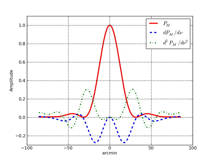
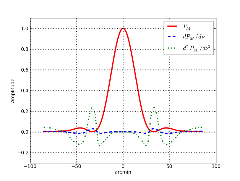
Figure 1.— The plot in the left panels shows the one dimensional cuts through the PB model at a reference frequency (continuous red line) for the VLA and its first (dashed blue line) and second derivatives (dash-dot green line) with respect to frequency. The plot on the right shows the same cuts through the $P_{eff}(\nu)$ – the effective frequency-independent PB.

3. The WB A-Projection algorithm

${adj\left({\mathsf{A}}_{k}\right)}$, when used in the A-Projection algorithm, corrects for the polarization and other DD effects that can be encoded in the phase of ${\mathsf{A}}^{\circ}$ (e.g. time-varying gains due to polarization squint, ionospheric phase-screen, etc.). It is however not a conjugate operator for variations along the time or frequency axis.

The image domain effects of the time varying gains are largely in the amplitude scaling only (i.e., they do not disperse the flux in the image domain). Since the minor cycle algorithms typically assume that the sky brightness distribution is time-invariant and do not parametrize the model image in time, the effects of such variations can be ignored in the transform from data to image domain. If the deviations from the average value are small (e.g. for antenna arrays and long integrations where time variability is cyclic, or antennas with three-axis mounts where beams do not rotate on the sky) the model prediction stage, which properly includes these effects, corrects for time variability in an the iterative deconvolution scheme.

Frequency dependence of ${\mathsf{A}}^{\circ}$ also varies with time (and direction). This variation is not cyclic and its maximum deviation from the average value increases with fractional bandwidth. Due to this, as for time varying gains, while the frequency dependence of ${\mathsf{A}}^{\circ}$ in the inner part of the main lobe of the PB can also be corrected via the model prediction stage, the convergence is significantly slower (requiring more major cycles and hence higher computing). Alternatively, this frequency dependence can be absorbed, to some extent, in the multi-term MFS (MT-MFS) minor cycle algorithm which solves for the time-invariant frequency dependence in the image plane. But this requires more Taylor-terms, which also is inadvisable (see section 4.3.3).

Correction for the time-variable frequency dependent effects of ${\mathsf{A}}^{\circ}$ requires a wide-band version of the ${\mathsf{A}}^{M}$ matrix such that ${adj\left({{\mathsf{A}}}^{M}_{k}\right)}\star{{\mathsf{A}}}^{\circ}_{k}$ results in a function which does not vary with frequency (i.e., ${adj\left({\mathsf{A}}^{M}\right)}$ is also a conjugate operator for frequency). The frequency dependence will then be projected-out prior to accumulation, resulting in an image corrected for the frequency dependent effects of ${\mathsf{A}}$.

3.1. The wide-band ${\mathsf{A}}$ operator

For the reasons givens above, as well as to keep the parameters for modeling the instrumental effects in the data domain separate from parameters for modeling the sky brightness distribution, we need to construct the ${\mathsf{A_{*}}}(\nu)$ matrix which projects-out the dependence on frequency during imaging. One such possibility is the following:

$${\mathsf{A_{*}}}(\nu)={\mathsf{F}}^{-1}\left[\frac{P_{eff}(\nu)P^{*}_{eff}(\nu)}{P(\nu)}\right]$$ (10)

where $P(\nu)={\mathsf{F}}^{{\dagger}}{\mathsf{A}}(\nu)$ and $P_{eff}(\nu)$ is the desired effective PB which varies minimally with frequency. In the data domain, ${adj\left({\mathsf{A}}_{*}(\nu)\right)}\star{\mathsf{A}}(\nu)$ can be shown to be frequency-independent to high orders, and this use of ${\mathsf{A_{*}}}(\nu)$ as a model for ${\mathsf{A}}(\nu)$ in the reverse transform can correct for the frequency dependence of ${\mathsf{A}}(\nu)$. However it also has a large support size, and therefore, in itself, is not an efficient reverse transform operator.

3.2. The Conjugate frequency

Equation 10 is valid for any frequency dependence. For the special case of PB scaling with frequency, we explore usable approximations for ${\mathsf{A_{*}}}$, we define the conjugate frequency $\nu_{*}$, given by:

$$\nu_{*}=\sqrt{2\nu_{ref}^{2}-\nu^{2}}$$ (11)

where $\nu_{ref}$ is the reference frequency of the continuum image, and examine the effects of choosing ${\mathsf{A}}_{*}(\nu)\equiv{\mathsf{A}}(\nu_{*})$.

Using the same model for ${\mathsf{A}}$ as used in Paper-I (i.e. a model for the VLA antenna PB), one dimensional cuts through the model PB given by $P_{M}(\nu)={\mathsf{F}}A(\nu)$, the effective PB given by $P_{eff}(\nu)={\mathsf{F}}\left[A(\nu_{*})\star A(\nu)\right]/\left[{\mathsf{F}}A(\nu_{ref})\right]$ and the first and second derivatives of $P_{eff}(\nu)$ with respect to frequency are shown in Fig. 1. A comparison of the derivatives of $P(\nu)$ and $P_{eff}(\nu)$ with frequency, shown in the two panels as blue dashed lines, shows that the effective PB is frequency-independent to the first order. While it changes in structure, the maximum second derivative remains almost the same in magnitude. These figures show that the approximation in Eq. 11 and use of ${\mathsf{A}}(\nu_{*})$ is good enough for imaging data which are not sensitive to the higher order frequency dependent effects. This approximation is useful since it can be easily implemented, is appropriate for the sensitivity of current telescopes and covers a large fraction of scientific observations for simultaneous Stokes-I and spectral index mapping. The frequency dependence in ${\mathsf{A}}(\nu)$ is reduced overall by an order of magnitude. When used in the A-Projection algorithmic steps in section 2.1.2, it effectively corrects for the frequency dependence of the PB prior to the accumulation along the frequency axis in Eq. 7. For future, more sensitive telescopes which will be sensitive to second order frequency dependent effects also, ${\mathsf{A_{*}}}$ as in Eq. 10 may be required. However, when software implementation itself requires partitioning along the time and/or frequency axis, hybrid approaches discussed in section 4 may be more efficient.

In practice, there might be multiple terms that make up the A-term, some of which may scale with frequency while others may not. E.g. Aperture Illumination will scale with frequency, but pointing-offset term or resonances effects will not. The terms that do not scale with frequency can be applied as multiplicative terms to ${\mathsf{A}}(\nu_{*})$ during gridding. We have tested this approach to work for parallel hand polarization effects. While we have not tested it, we think this may also work for cross-hand polarizations.

To avoid confusion and for brevity, we will refer to the algorithm in Paper-I as the Narrow-band A-Projection  or NB A-Projection algorithm, and refer to the use of ${\mathsf{A}}(\nu_{*})$ (instead of ${\mathsf{A}}(\nu)$) for the data-to-image domain transform as the WB A-Projection algorithm.

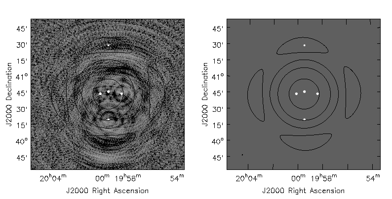
Figure 2.— This figure shows imaging performance before and after applying corrections for the time and frequency dependence of the PB during imaging. The sky is assumed to have a flat-spectrum, and standard MFS imaging is done. Both restored images are shown at the same gray-scale, stretched to emphasize artifacts. Contours are drawn at the 0.02, 0.1 and 0.5 (HPBW) levels of the time-and-frequency averaged Primary Beam. No noise was added to the simulated visibilities, in order to clearly illustrate the noise-like artifacts produced by time-variable DD-effects.
LEFT : Standard MFS-imaging and deconvolution, using a prolate-spheroidal gridding convolution function. Dominant errors are due to the time and frequency variability of the PB. Off-source RMS : $4\times 10^{-4}Jy$, Peak Residual : $1.8\times 10^{-3}Jy$
RIGHT : MFS-imaging and deconvolution, using WB A-Projection to account for both time and frequency variability during gridding. Off-source RMS : $1.5\times 10^{-7}Jy$, Peak Residual : $7\times 10^{-7}Jy$

3.3. Algorithm Validation

The image deconvolution algorithm described in section 3 was tested using simulated wide-band data with 66% fractional bandwidth. The VLA C-array was used for antenna configuration and the observations covered Hour Angle range of $\pm 3^{h}$. The model for the PB used in Paper-I was scaled by frequency and rotated with Parallactic Angle to simulate time-varying frequency dependent effects. To clearly highlight the effects of time and frequency dependence of ${\mathsf{A}}$, we used a model of the sky consisting of five point sources located at 0.99, 0.83, 0.60 and 0.11 levels of the PB within the main lobe and one source located in the first side lobe (PB gain of 0.025). All the point sources were assigned a flux of 1 Jy with flat spectra. The effective spectral-indices due to the primary-beam at the five locations are -0.026,-0.38, -1.0,-5.32 and +0.47 respectively. No noise was added to these simulations, and all imaging and deconvolution runs were with a loop-gain of 0.2.

Figure 2 shows deconvolved images produced without (first panel) and with (second panel) WB A-Projection gridding. This comparison demonstrates that with an accurate model of the Primary Beam, it is possible to correct-for its time- and frequency-variability down to numerical precision levels in wide-band wide-field imaging.

4. Applying NB A-Projection for wide-band imaging

NB A-Projection was designed for a single reference frequency and does not automatically account for the frequency-dependence of P during gridding. However, it can still be used for wide-band imaging, as long as the frequency dependence of the far-field pattern is known and characterized by $P_{\nu}$. Several algorithmic options exist, all with different numerical approximations and computing load. This flexibility allows the implementation to be tuned according to the available computing resources, architecture of the hardware platform and the desired imaging accuracy.

4.1. Cube imaging + Cube deconvolution

The simplest approach is spectral-cube imaging where each frequency channel (with its limited $uv$ coverage) is treated separately. NB A-Projection is applied as is per channel, and the minor cycle run independently per channel. A continuum image is later constructed by adding together deconvolved and restored images from all channels.

The residual image per channel can be approximately re-written from Eq. 7 in the image domain, for the case where the aperture illumination functions are identical for all baselines and times, and only one polarization-pair is being imaged.

$$I^{R}_{\nu}={{{{P_{\nu}}\cdot\left(I^{psf}_{\nu}\star\left({P_{\nu}}\cdot I^{sky}_{\nu}\right)\right)}}\over{{P_{\nu}}^{2}}}$$ (12)

where $I^{psf}_{\nu}=F^{-1}\sum_{k}\delta_{k,\nu}$ ($k\equiv ij,t$) is the point spread function for one channel and ${P_{\nu}}=F^{-1}A_{\nu}$. In this expression, the division by ${P_{\nu}}^{2}$ implies a flat-sky normalization, but a flat-noise normalization may be used instead.

This method is straightforward and will suffice for modest imaging dynamic ranges and uncomplicated spatial structure (point sources). However, the angular resolution of the continuum image and any estimate of the sky spectrum will be limited to that of the lowest frequency in the band. Also, reconstruction uncertainties may be inconsistent across frequency when there is insufficient $uv$-coverage per channel or complicated spatial structure, leading to spurious spectral structure.

In this paper, we are focusing on imaging problems that require more accuracy and dynamic-range than what the above offers. In the next two sections, we discuss A-Projection in the context of multi-frequency-synthesis (MFS) where the combined $uv$-coverage is used for model reconstruction (minor cycle).

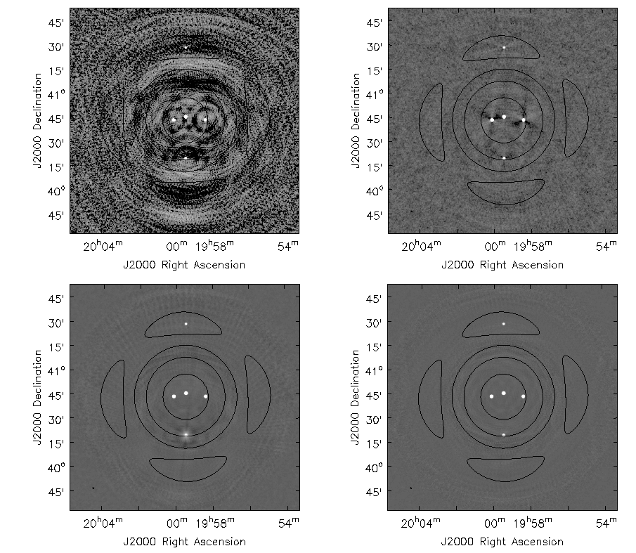
Figure 3.— These figures compare the imaging performance before and after applying corrections for the time and frequency dependence of the PB during imaging. All restored images are shown at the same gray-scale, stretched to emphasize artifacts. Contours are drawn at the 0.02, 0.1 and 0.5 (HPBW) levels of the time-and-frequency averaged Primary Beam. Results from four algorithms described in Sec. 4.3 are compared here (MFS+SI, MT-MFS+SI, MT-MFS+A-Projection, MT-MFS+WB A-Projection). RMS and peak-residuals are listed in the table below.

Panel	Algorithm	Description	RMS	Peak Residual	Comments
			(Jy/beam)	(Jy/beam)
Top Left	MFS + SI	Standard Wide-band Imaging	$6\times 10^{-4}$	$2.3\times 10^{-3}$	Ignore time & frequency dependence. Artifacts due to time and frequency variations of the PB.
Top Right	MT-MFS+ SI	Multi-term Imaging with Standard Gridding	$1\times 10^{-4}$	$5\times 10^{-4}$	Ignore time dependence. Absorb time-averaged frequency dependence in MT-MFS. Artifacts due to time-variability of the PB.
Lower Left	MT-MFS+ A-Projection	Multi-term Imaging with NB A-Projection gridding	$4\times 10^{-5}$	$8\times 10^{-4}$	Account for time variability of PB, and absorb the resulting $PB^{2}$ frequency dependence in MT-MFS. Artifacts due to stronger spectral structure.
Lower Right	MT-MFS+ WB A-Projection	Multi-term Imaging with wide-band A-Projection gridding	$3.5\times 10^{-5}$	$2\times 10^{-4}$	Account for PB time- & frequency-dependence in WB A-Projection. Account for static sky-frequency dependence in MT-MFS. Minimal artifacts.

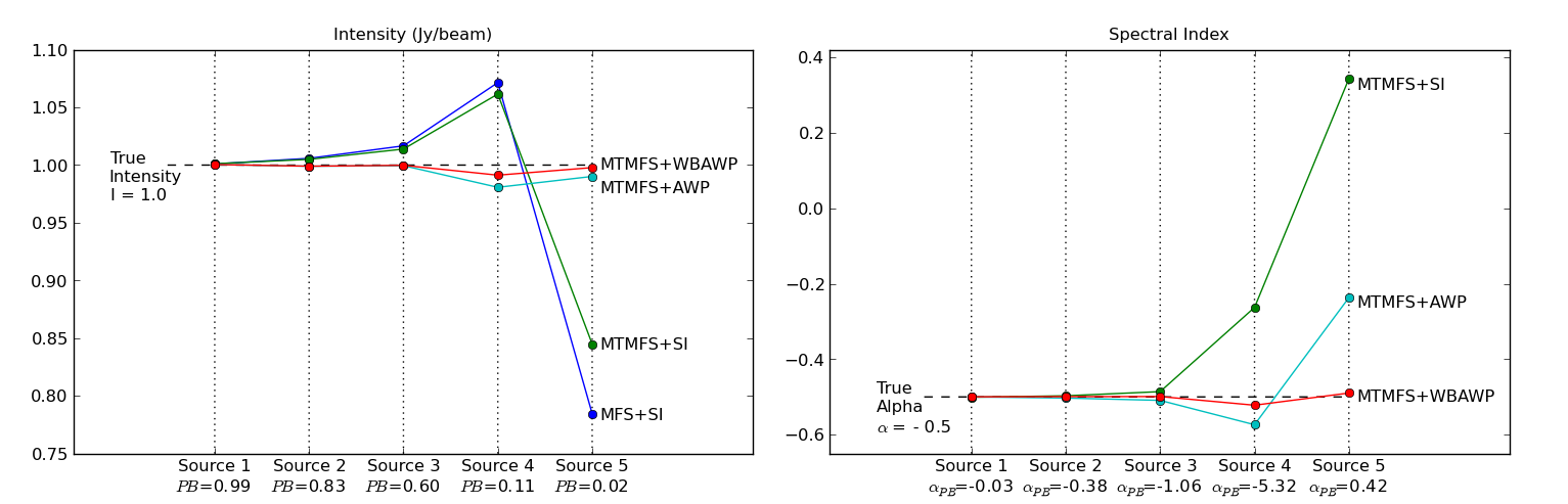
Figure 4.— This figure compares the accuracy of the PB-corrected intensity (LEFT) and spectral-index (RIGHT) for the five simulated point sources, using the four methods whose results are shown in Figure 3. The labels “AWP” and “WBAWP” are used for A-Projection and WB A-Projection in the figure. The algorithms compared are MFS+SI, MT-MFS+SI, MT-MFS+A-Projection and MT-MFS+WB A-Projection. Spectral-indices are shown only for methods using MT-MFS, with post-deconvolution (average) spectral-index corrections done for the SI and A-Projection runs. Results for the five sources are shown from left to right with increasing distance from the pointing-center. The reference-PB gain and effective PB-spectral-index at the locations of the five sources are listed on the x-axis. These plots show that outside the HPBW at the reference-frequency, methods that do not account for time-variable PB-spectra have considerably higher errors, and the combination of MT-MFS+WB A-Projection delivers accurate corrections even out in the sidelobe.

4.2. Cube imaging + MFS deconvolution

The simplest extension of NB-A-Projection for multi-frequency synthesis is to grid, Fourier transform and normalize each frequency channel (or sets of channels) independently, and then produce a continuum image by an image-domain accumulation, before the minor cycle. When the sky spectrum is not flat, or when flat-noise normalization is used per channel, a wide-band minor-cycle algorithm such as MT-MFS can be applied to simultaneously solve for the sky intensity and spectrum. Taylor-weighted residual images are constructed as follows, before proceeding to the minor cycle.

$$I^{R}_{t}=\sum_{\nu}{w_{\nu}^{t}}I^{R}_{\nu}=\sum_{\nu}{w_{\nu}^{t}}\left\{{{P_{\nu}}\cdot\left({I_{\nu}}^{psf}\star\left({P_{\nu}}\cdot{I_{\nu}}^{sky}\right)\right)}\over{{P_{\nu}}^{2}}\right\}$$ (13)

where ${w_{\nu}^{t}}={\left({\nu-\nu_{0}}\over{\nu_{0}}\right)}^{t}$ are weights that represent Taylor polynomial basis functions (Rau & Cornwell 2011). The interpretation of the output Taylor coefficients depends on the choice of normalization as follows.

1. With flat-sky normalization per channel, the output Taylor coefficients will represent $I^{sky}_{\nu}$.

2. For flat-sky normalization per channel, but a regularized flat noise minor cycle, the Taylor-weighted residual images can be multiplied by a $P_{ref}$ after the frequency summation and before deconvolution. The output Taylor coefficients will represent $P_{ref}I^{sky}_{\nu}$ and a post-deconvolution division by $P_{ref}$ will be required for the intensity image. No corrections are needed for the spectral index map.

3. With flat-noise normalization per channel before Taylor-weighted averaging, the output Taylor coefficients will represent $P_{\nu}I^{sky}_{\nu}$, and a post-deconvolution polynomial division of the primary beam spectrum will be required to correct both the intensity and the spectral index.

Qualitatively, the reverse transform with flat-sky normalization per channel followed by frequency-averaging and a flat-noise regularization by $P_{ref}$ before the minor cycle, is equivalent to the use of WB A-Projection during gridding. It requires multiple image grid planes (one per channel), FFTs and has repeated beam divisions and multiplications that can increase numerical errors. However, it is naturally parallelizable, making it an attractive option for extremely large data sets and imaging goals where inaccuracy in low gain regions of the primary beam can be tolerated.

4.2.1 MFS imaging + MFS deconvolution

To optimize on memory use and FFT costs (especially in a non-parallel imaging run), MFS gridding can be done, where averages over baseline, time and frequency are accumulated onto a single grid, followed by a single FFT and normalization by an average primary beam (or its square). Here, attention must be paid to the consequences of averaging over frequency before normalization. The use of ${adj\left({\mathsf{A}}(\nu)\right)}$ as the gridding convolution function (the NB-A-Projection algorithm), introduces an additional frequency dependence $P_{\nu}$ that gets averaged over before it can be removed. Once gridded, this extra frequency dependence is locked in, and can be accounted for only as an artificially steeper spectrum in the minor-cycle of the MT-MFS wide-band imaging algorithm.

Multi-term Taylor-weighted residual images must be constructed as follows,

$$I^{R}_{t}={{\sum_{\nu}{w_{\nu}^{t}}\left\{{{P_{\nu}}\cdot\left({I_{\nu}}^{psf}\star\left({P_{\nu}}\cdot{I_{\nu}}^{sky}\right)\right)}\right\}}\over{\sum_{\nu}{P_{\nu}}^{2}}}$$ (14)

and the output Taylor coefficients will depend on the choice of normalization as follows

1. For flat-sky normalization, the model intensity represents $I^{sky}_{ref}$, but the spectrum represents the product of the sky spectrum and the square of the primary-beam spectrum.

2. For flat-noise normalization, the model intensity represents $I^{sky}_{ref}P_{avg}$ and the spectrum represents the product of the sky spectrum and the square of the primary beam spectrum.

In both cases, appropriate wide-band post-deconvolution corrections for the average primary beam and two instances of the primary beam spectrum, must be applied.

Such corrections are inelegant, and are susceptible to numerical instabilities in low gain regions of the primary beams. Section 4.3 shows a comparison of some of these methods with WB A-Projection, for a simulation with source spectra that are not flat and therefore require MT-MFS imaging and deconvolution.

4.3. Comparison of Hybrids with WB A-Projection

To test the algorithm described in sections 3 and 3.1 with non-flat source spectra, we used the sky brightness distribution as in Fig. 2, but assigned a spectral index of $\alpha=-0.5$ to all sources such that $I(\nu)\propto(\nu/\nu_{o})^{\alpha}$.

Figure 3 shows deconvolved images produced with and without time-dependent and frequency-dependent PB-corrections during gridding, emphasizing the different types of error-patterns that arise when one or more effects are ignored. An image formed from the hybrid method described in Sec. 4.2.1 to absorb all frequency-dependence into the minor cycle solver is also shown for comparison. Figure 4 shows Stokes-I and spectral index values for these point-sources after PB-correction, to illustrate the accuracy to which different methods are able to recover the true-sky spectral index at various locations in the PB. The various methods tested and results obtained are described below.

4.3.1 MFS + SI (Standard Imaging)

The image in the top left panel of Fig. 3 is the result of standard Cotton-Schwab Clean with MFS gridding using prolate-spheroidal functions as gridding-convolution functions, and a flat-spectrum assumption during the minor cycle.

$$I^{R}=\sum_{\nu}\left\{{\left({I_{\nu}}^{psf}\star\left({P_{\nu}}\cdot{I_{\nu}}^{sky}\right)\right)}\right\}$$ (15)

Time and frequency variability of both the sky and the instrument are ignored, and for a 66% bandwidth, imaging artifacts around all sources away from the pointing-center are dominated by spectral-effects due to $P_{\nu}$ present in the data. A post-deconvolution division by an average primary beam can recover the true source intensity to within a few percent, out to the half-power point of the PB, but errors increase with distance from the pointing center.

4.3.2 MT-MFS + SI

The image in the top right panel of Fig. 3 is the result of the MT-MFS algorithm in the minor cycle, with standard gridding (prolate-spheroidal functions). The minor cycle solves for the average intensity and spectrum of $I(\nu)P(\nu)$ using a 2-term Taylor-polynomial approximation.

$$I^{R}_{t}=\sum_{\nu}{w_{\nu}^{t}}\left\{{\left({I_{\nu}}^{psf}\star\left({P_{\nu}}\cdot{I_{\nu}}^{sky}\right)\right)}\right\}$$ (16)

Average PB-spectral effects are absorbed into the sky model, and the dominant remaining error is due to the time-variability of the primary-beams. A post-deconvolution correction of the continuum intensity and spectral-index are accurate to within a few percent in intensity and $\pm$0.1 in spectral index out to approximately the half-power point. Beyond this field-of-view, errors increase (to $\pm 0.4$ or more in spectral index) primarily because a time-averaged primary-beam spectrum is not a good estimate in regions of the image where $P_{\nu}$ changes by 100% with time as the beams rotate on the sky.

4.3.3 MT-MFS + A-Projection

The image in the bottom left panel of Fig. 3 is the result of MT-MFS in the minor cycle (2 terms), but with the NB A-Projection gridding as described in Sec. 4.2.1 with a flat-noise normalization before the minor cycle, followed by a post-deconvolution correction of the intensity by $P_{ref}$ (average primary beam) and the spectral index by twice that of the primary beam. Artifacts due to frequency-independent time-variability (antenna rotation) no-longer exist within the HPBW (PB gain of 0.5), but new spectral artifacts appear away from the pointing-center (beginning around the 10% level).

These errors are partly due to the increased non-linearity of the $P^{2}(\nu)$ spectrum away from the pointing center, for which a two-term Taylor-polynomial approximation is insufficient. A run with 3 terms partially reduces this problem, indicating that errors in approximating the combined spectrum with a low-order polynomial dominates the errors, but higher order polynomials are inadvisable because of instability in low-SNR regions.

Errors also arise from the high time variability of the PB-spectrum, which is ignored because only time-averaged spectra are used for spectral-correction. A post-deconvolution correction of the spectral-index map for $P^{2}(\nu)$ results in errors at the $\pm 0.3$ level beyond the $\sim$50% point.

4.3.4 MT-MFS + WB A-Projection

The image in the bottom right panel of Fig. 3 is the result of MT-MFS in the minor cycle (two terms), and WB A-Projection gridding (section 3). Artifacts around all sources are gone, and the dominant errors are numerical (at the floating-point precision level). The spectral-index map produced by MT-MFS is accurate to within 0.01 in the main lobe, and 0.05 out in the sidelobe. Such accuracies allows the recovery of source-spectra further-out in the primary-beam than previously possible. The main difference between this method and all others, is that time and frequency variability of the primary beam has been corrected for in the data domain, before any averaging is done to construct a continuum image to send to the minor cycle. The minor cycle sees a flat-noise normalization, preserving the convolution-equation and allowing for deeper ’cleaning’ before triggering the next major cycle (i.e. faster convergence).

This method shows the lowest errors in Fig. 4 indicating that if the primary beam can be accurately modeled, its time and frequency variability can be corrected for during gridding, resulting in an accurate reconstruction in the minor cycle.

4.4. Imaging results with VLA L-Band data

Figure 5 shows the continuum intensity and spectral index distribution of the G55.7+3.4 Galactic supernova remnant (SNR), using the VLA in L-band and D-configuration and made with and without the WB A-Projection algorithm. The peak brightness is 6mJy, and with an off-source RMS of 11 $\mu$Jy, this is a modest dynamic range. The peak brightness comes from a background pulsar with a known spectral index of -2.3, and the brighter synchrotron-emission filaments are at the 1mJy level. The half-power beam width (HPBW) of the PB is 30 arcmin, and extended emission from the SNR fills the PB at the reference frequency. The spurious spectral index at the HPBW due to the primary beam variation between 1-2 GHz is approximately -1.4.

The left column of panels in Fig. 5 shows continuum intensity, and the right column shows corresponding spectral index maps.

1. The top row shows flat-noise results with MTMFS+SI, where A-Projection was not used, and primary-beam correction was not done. There is considerable artificial steepening (darkening on the plot) of the observed source spectrum as distance from the pointing center increases. The spectral index of the bright background pulsar is -3.05.

2. The middle row shows flat-sky results from the same run as above, where MTMFS+SI was followed by a post-deconvolution wideband PB correction of both the intensity and the spectrum. The spectral index map shows that this post-deconvolution correction has restored the spectral indices of the outer part of the SNR as well as the background sources to more realistic values. The spectral index of the bright background pulsar is -2.61 (after correction for an average estimated PB spectral index of -0.44 at the 0.8 gain level).

3. The bottom row shows flat-sky results from an MTMFS+WBAWP run where the intensity image has been corrected for the average PB gain, but the spectral index image is just what came out of the imaging run. The noise properties of the intensity image are slightly better than the middle row, and the spectral index map shows slightly more coherent and less noisy structure across the SNR. The spectral index of the bright background pulsar is -0.29, which is the closest so far to the expected value.

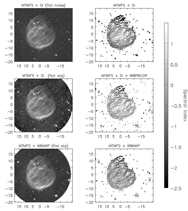
Figure 5.— The left column shows wide-band continuum Stokes-I images of the Galactic SNR G55 imaged with the VLA centered at 1.5 GHz covering the frequency range $1.256-1.905$ GHz. The right column shows the spectral index maps. The top and middle rows are the results from MTMFS+SI imaging, without and with a post-deconvolution wideband PB-correction respectively. The artificially high spectral index around the edge of the SNR emission and farther out, in the top row, is due to the PB. This is not present in the middle row, but the spectral index map is still noisy. The bottom row shows the flat-sky results from MTMFS+WBA-Projection with spectral indices closer to their expected values than either of the other methods. Details are discussed in Sec. 4.4.

5. Conclusions

In this paper we describe the wide-band A-Projection (WB A-Projection) algorithm, which extends the narrow-band A-Projection (NB A-Projection) algorithm (Bhatnagar et al. 2008) to correct for the wide-band effects of the PB prior to integration in time and frequency for continuum imaging. We demonstrate that the combined WB A-Projection and MT-MFS algorithm for simultaneous intensity and spectral index mapping performs as expected.

Theoretical analysis in section 2.1.2 draws equivalence between standard antenna complex gain and bandpass calibration and the NB A-Projection and WB A-Projection algorithms respectively and show that the latter two algorithms are the direction-dependent generalization of the former direction-independent algorithms. The A-term of the A-Projection algorithm represents the direction-dependent (DD) complex antenna gain pattern in the data domain. Since it is direction-dependent, corrections for it fundamentally cannot be decoupled from imaging and must be corrected for during imaging (see Rau et al. 2009). The A-Projection algorithm, which corrects for the DD antenna gains during imaging, therefore can be thought of as an algorithm for DD calibration. Similarly, the WB A-Projection algorithm which includes corrections for the frequency dependence of the A-term can be thought of as the DD generalization of the standard bandpass calibration algorithm. We feel that making these connections with simpler, intuitively better understood and widely used algorithms in the community makes it easier to understand the newer more general techniques.

We also analyzed hybrid schemes for wide-band imaging using the NB A-Projection and image-plane correction for the effects of PB. Our conclusion is that while for non-parallel implementation, WB A-Projection is required for wide-band imaging, for implementations which may require partitioning the data along time and/or frequency axis, hybrid approaches are also sufficient. However the use of WB A-Projection in implementations on parallel processing platforms allows the freedom to tune the distribution of the data to suite the available hardware and computing resources (e.g., this allows imaging smaller chunks of the total bandwidth in parallel, even if these smaller chunks need wide-band PB corrections. Without WB A-Projection, the data distribution is restricted to be partitioned in frequency such that each chunk can be imaged using NB A-Projection).

Comparisons show that the WB A-Projection plus MT-MFS enables simultaneous intensity and spectral index imaging throughout the PB in wide-field imaging. Moderate dynamic range imaging within the half-power point of the PB is possible where all frequency dependence in the image is absorbed in the solution of the MT-MFS algorithm. Beyond this field-of-view (FoV), errors increase because a time-averaged primary-beam spectrum is not a good estimate in regions of the image where PB changes by 100% with time as the beams rotate on the sky. The FoV can be increased till $\sim 10\%$ point of the PB by combining MT-MFS with NB A-Projection. The time-dependence of the PB is accounted for via A-Projection and its frequency dependence is absorbed in MT-MFS. Using larger number of Taylor-terms in MT-MFS improves the imaging performance for simpler fields, but is inadvisable because of instability in low-SNR regions.

Finally, we would like to note that while only the effects of the antenna PB were included in the A-term used in this paper, other antenna-based DD effect can also be easily included. The effect of non-isoplanatic ionospheric/atmospheric phases is comparable to the effect of PB for wide-band wide-field imaging at low frequencies, particularly with aperture-array antenna elements. Similar effects come from the irregularities in the water vapor content in the lower atmosphere for imaging at high frequencies. The effects due to ionosphere/atmosphere and PB need to be corrected simultaneously, often for wide-band data in full polarization. It may be possible to extend the WB A-Projection algorithm presented here to include corrections for ionospheric effects. Work to test these extensions is underway and will be reported in future publications.

References

- Bhatnagar et al. (2008) Bhatnagar, S., Cornwell, T. J., Golap, K., & Uson, J. M. 2008, Astron. & Astrophys., 487, 419
- Cornwell (1995) Cornwell, T. J. 1995, The Generic Interferometer: II Image Solvers, Tech. rep., AIPS++ Note 184
- Hamaker et al. (1996) Hamaker, J. P., Bregman, J. D., & Sault, R. J. 1996, Astron. & Astrophys. Suppl. Ser., 117, 137
- Rau et al. (2009) Rau, U., Bhatnagar, S., Voronkov, M. A., & Cornwell, T. J. 2009, Proc. IEEE, 97, No. 8, 1472
- Rau & Cornwell (2011) Rau, U., & Cornwell, T. J. 2011, A&A, 532, A71