Generalized Multiscale Finite Element Methods. Nonlinear Elliptic Equations

Abstract

In this paper we use the Generalized Multiscale Finite Element Method (GMsFEM) framework, introduced in [20], in order to solve nonlinear elliptic equations with high-contrast coefficients. The proposed solution method involves linearizing the equation so that coarse-grid quantities of previous solution iterates can be regarded as auxiliary parameters within the problem formulation. With this convention, we systematically construct respective coarse solution spaces that lend themselves to either continuous Galerkin (CG) or discontinuous Galerkin (DG) global formulations. Here, we use Symmetric Interior Penalty Discontinuous Galerkin approach. Both methods yield a predictable error decline that depends on the respective coarse space dimension, and we illustrate the effectiveness of the CG and DG formulations by offering a variety of numerical examples.

1 Introduction

Nonlinear partial differential equations represent a class of problems that have applications in many scientific communities [16, 35]. Forchheimer flow and nonlinear elasticity are two particular examples of physical processes that are modeled by nonlinear equations [14, 27]. In addition to difficulties associated with the nonlinearity, these types of problems often involve coefficients that exhibit high-contrast, heterogeneous behavior. For example, when modeling subsurface flow, the underlying permeability field is often represented by a high-contrast coefficient in the pressure equation. One approach for solving a high-contrast, nonlinear equation is to linearize the problem and use an iterative method for obtaining the solution. For example, a Picard iteration yields an iterative process where a previous solution iterate is directly used in order to update the solution at the current iteration. In this case, a final solution is obtained when a suitable tolerance between the current and previous iteration is reached. While relatively easy to implement, iterative techniques typically require a repeated number of solves in order to obtain a convergent solution. In the case of a nonlinear elliptic equation, each iteration requires the numerical solution of a large system of equations that depends on the previous iterate. Thus, computing solutions on a fully resolved mesh quickly becomes a prohibitively expensive task. As such, techniques that allow for a more efficient computational procedure with a suitable level of accuracy are desirable.

The past few decades have seen the development of various multiscale solution techniques for capturing small scale effects on a coarse grid [1, 3, 24, 28, 29, 30]. The multiscale finite element methods (MsFEM’s) that we consider in this paper hinge on the construction of coarse spaces that are spanned by a set of independently computed multiscale basis functions. The multiscale basis functions are then coupled via a respective global formulation in order to compute the solution. In particular, solutions may be computed on a coarse grid while maintaining the fine-scale effects that are embedded into the basis functions. While standard multiscale methods have proven effective for a variety of applications (see, e.g., [23, 24, 25, 30]), in this paper we consider a more recent framework in which the coarse spaces may be systematically enriched to converge to the fine grid solution [5, 21, 22, 34]. More specifically, additional basis functions are chosen based on localized eigenvalue problems that capture the underlying behavior of the system. In this case, we may carefully choose the number of basis functions (and dimension of the coarse space) such that we achieve a desired level of accuracy. In this paper we additionally show that the systematic enrichment of coarse spaces is flexible with respect to the global formulation that is chosen to couple the resulting basis functions.

To treat the nonlinear elliptic equation considered in this paper we make use of the Generalized Multiscale Finite Element Method (GMsFEM) which was introduced in [20]. In order to do so, we apply a Picard iteration and treat an upscaled quantity of a previous solution iterate as a parameter in the problem. With this convention we follow an offline-online procedure in which the coarse space construction is split into two distinct stages; offline and online (see [8, 10, 34, 37]). The main goal of this approach is to allow for the efficient construction of an online space (and an online solution) for each fixed parameter value and iteration. In the process, we precompute a larger-dimensional, parameter-independent offline space that accounts for an appropriate range of parameter values that may be used in the online stage. As construction of the offline space will constitute a one-time preprocessing step, only the online space will require additional work within the solution procedure. In the offline stage we first choose a fixed set of parameter values and generate an associated set of “snapshot” functions by solving localized problems on specified coarse subdomains. The functions obtained through this step constitute a snapshot space which will be used in the offline space construction. To construct the offline space we solve localized eigenvalue problems that use averaged quantities of the parameter(s) of interest within the space of snapshots. We then keep a certain number of eigenfunctions (based on some criterion) to form the offline space. At the online stage we solve similar localized problems using a fixed parameter value within the offline space, and keep a certain number of eigenfunctions for the online space construction.

In this paper we consider the continuous Galerkin (CG) and discontinuous Galerkin (DG) formulations for the global coupling of the online basis functions. We show that each method offers a suitable solution technique, however, at this point we highlight some distinguishing characteristics of the repsective methods as motivation for considering both formulations. For the nonlinear elliptic equation considered in this paper, the CG coupling yields a bilinear form that closely resembles the standard finite element method (FEM). In particular, the integrations that define the CG formulation are taken over the whole domain, and result in a reduced-order system of equations that is similar in nature to the fine-scale system. As such, the ease of implementation, classical FEM analogues, and well understood structure make CG a tractable method for coupling the coarse basis functions in order to solve the global problem [28]. While the discontinuous Galerkin formulation is arguably more delicate than its CG counterpart, DG offers an attractive feature such as it does not require partition of unity functions to couple basis functions. Both methods are shown to be suitable coupling mechanisms within the GMsFEM framework that is described in this paper. In particular, an increase in the size of the online coarse space yields a predictable error decline, and the error is shown to behave according to previous error estimates that depend on the eigenvalue behavior. The flexibility of the coarse space enrichment, along with the choice of using CG or DG as the global coupling mechanism, makes GMsFEM a robust and suitable technique for solving the model equation that we consider in this paper. A variety of numerical examples are presented to validate the performance of the proposed method.

We note that some numerical results for GMsFEM in the context of continuous Galerkin methods for nonlinear equations are presented in [20]. These numerical results are mostly presented to demonstrate the main concepts of GMsFEM and we do not have careful studies for nonlinear problems in [20]. Moreover, the numerical results presented in [20] use reduced basis approach to identify dominant eigenmodes which is different from the local mode decomposition approach presented here. Moreover, the current paper also studies DG approach for nonlinear equations.

The organization of the paper is as follows. In Sect. 2 we introduce the model problem, the iterative procedure, and notation to be used throughout the paper. In Sect. 3 we carefully describe the coarse space enrichment procedure, and introduce the continuous and discontinuous Galerkin global coupling formulations. In particular, Subsect. 3.1 is devoted to the offline-online coarse space construction, and in Subsect. 3.2 we describe the CG and DG global coupling procedures. A variety of numerical examples are presented in Sect. 4 to validate the performance of the proposed approaches, and in Sect. 5 we offer some concluding remarks.

2 Preliminaries

In this paper we consider non-linear, elliptic equations of the form

$$-\mbox{div}\big{(}\kappa(x;u)\,\nabla u\big{)}=f\,\,\text{in}\,D,$$ (1)

where $u=0$ on $\partial D$. We assume that $u$ is bounded above and below, i.e., $u_{0}\leq u(x)\leq u_{N}$, where $u_{0}$ and $u_{N}$ are pre-defined constants. We will also assume that the interval $[u_{0},u_{N}]$ is divided into $N$ equal regions whose endpoints are given by $u_{0}<u_{1}<...<u_{N-1}<u_{N}$.

In order to solve Eq. (1) we will consider a Picard iteration

$$-\mbox{div}\big{(}\kappa(x;u^{n}(x))\,\nabla u^{n+1}(x)\big{)}=f\ \text{in}\ D,$$ (2)

where superscripts involving $n$ denote respective iteration levels. To discretize (2), we next introduce the notion of fine and coarse grids. We let $\mathcal{T}^{H}$ be a usual conforming partition of the computational domain $D$ into finite elements (triangles, quadrilaterals, tetrahedrals, etc.). We refer to this partition as the coarse grid and assume that each coarse subregion is partitioned into a connected union of fine grid blocks. The fine grid partition will be denoted by $\mathcal{T}^{h}$. We use $\{x_{i}\}_{i=1}^{N_{v}}$ (where $N_{v}$ the number of coarse nodes) to denote the vertices of the coarse mesh $\mathcal{T}^{H}$, and define the neighborhood of the node $x_{i}$ by

$$\omega_{i}=\bigcup\{K_{j}\in\mathcal{T}^{H};\leavevmode\nobreak\ \leavevmode\nobreak\ \leavevmode\nobreak\ x_{i}\in\overline{K}_{j}\}.$$ (3)

See Fig. 1 for an illustration of neighborhoods and elements subordinated to the coarse discretization. We emphasize the use of $\omega_{i}$ to denote a coarse neighborhood, and $K$ to denote a coarse element throughout the paper.

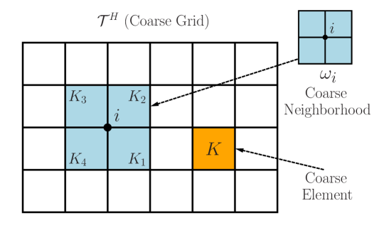
Figure 1: Illustration of a coarse neighborhood and coarse element

Next, we briefly outline the global coupling and the role of coarse basis functions for the respective formulations that we consider. For the discontinuous Galerkin (DG) formulation, we will use a coarse element $K$ as the support for basis functions, and for the continuous Galerkin (CG) formulation, we will use $\omega_{i}$ as the support of basis functions. To further motivate the coarse basis construction, we offer a brief outline of the global coupling associated with the CG formulation below. For the purposes of this description, we formally denote the CG basis functions by $\psi_{k}^{\omega_{i}}$. In particular, we note that the proposed approach will employ the use of multiple basis functions per coarse neighborhood. In turn, the CG solution at $n$-th iteration will be sought as $u^{\text{CG}}_{\text{ms}}(x;\mu)=\sum_{i,k}c_{k}^{i}\psi_{k}^{\omega_{i}}(x;\mu)$, where $\psi_{k}^{\omega_{i}}(x;\mu)$ are the basis functions for $n$-th iteration, and $\mu$ is used to denote dependence on the previous solution. We note that a main consideration of our method is to allow for rapid calculations of basis functions at each iteration.

Once the basis functions are identified, the CG global coupling is given through the variational form

$$a(u^{\text{CG}}_{\text{ms}},v;\mu)=(f,v),\quad\text{for all}\,\,v\in V_{\text{on}}^{\text{CG}},$$ (4)

where $V_{\text{on}}^{\text{CG}}$ is used to denote the space formed by those basis functions.

We also note that an appropriate set of basis functions defined on each coarse element $K$ may be respectively coupled via a discontinuous Galerkin formulation (see e.g., [4, 36, 15]).

3 CG and DG GMsFEM for nonlinear problems

3.1 Local basis functions

To motivate the local basis construction, we first introduce an approximation to the solution of Eq. (2) given by

$$-\mbox{div}\big{(}\kappa(x;\overline{u}^{n}(x))\nabla u^{n+1}(x)\big{)}=f\,\,\text{in}\,D,$$ (5)

where $\overline{u}$ denotes the average of $u$ in each coarse region (either $K$ or $\omega_{i}$, depending on the desired formulation). Because the variation in $\overline{u}^{n}$ is not known a priori, we use $\mu$ to represent the dependence of the solution on $\overline{u}^{n}$. As part of the iterative solution process, multiscale basis functions will be computed for a selected number of the parameter values at the offline stage, and we will compute multiscale basis functions for each new value of $\overline{u}^{n}$ at the online stage. In this section we will describe these details, and note that we maintain the convention of denoting $\overline{u}$ by the parameter $\mu$. We omit the iterative index $n$ (and $n+1$) for additional notational brevity, although note that the iterative process should be clearly implied.

With the notational conventions in place we now describe the offline-online computational procedure, and elaborate on some applicable choices for the associated bilinear forms to be used in the coarse space construction. Below we offer a general outline for the procedure.

• Offline computations:

  • 1.0. Coarse grid generation.

  • 1.1. Construction of snapshot space that will be used to compute an offline space.

  • 1.2. Construction of a small dimensional offline space by performing dimension reduction in the space of global snapshots.

• Online computations:

  • 2.1. For each input parameter, compute multiscale basis functions.

  • 2.2. Solution of a coarse-grid problem for any force term and boundary condition.

  • 2.3. Iterative solvers, if needed.

In the offline computation, we first construct a snapshot space $V_{\text{snap}}^{\tau}$, where $\tau$ denotes either a coarse neighborhood $\omega_{i}$ in the continuous Galerkin case, or a coarse element $K$ in the discontinuous Galerkin case (refer back to Fig. 1). Construction of the snapshot space involves solving the local problems for various choices of input parameters, and we describe the details below.

In order to construct the space of snapshots we propose to solve the following eigenvalue problem on a coarse domain $\tau$:

$$A(\mu_{j})\psi_{l,j}^{\tau,\text{snap}}=\lambda_{l,j}^{\tau,\text{snap}}S(\mu_{j})\psi_{l,j}^{\tau,\text{snap}}\quad\text{in}\,\,\,\tau,$$ (6)

where $\mu_{j}$ ($j=1,\dots,J$) is a specified set of fixed parameter values, and we again emphasize that $\tau$ denotes a different coarse subdomain (either a coarse neighborhood $\omega_{i}$ or coarse element $K$) depending on whether we consider the CG or DG problem formulation. We are careful to note that zero Neumann boundary conditions are generally used to solve eigenvalue problem, except in the DG case when Dirichlet conditions are used on element boundaries that coincide with the global domain. The matrices in Eq. (6) are defined as

$$A(\mu_{j})=[a(\mu_{j})_{mn}]=\int_{\tau}\kappa(x;\mu_{j})\nabla\phi_{n}\cdot\nabla\phi_{m}\quad\text{and}\quad S(\mu_{j})=[s(\mu_{j})_{mn}]=\int_{\tau}\widetilde{\kappa}(x;\mu_{j})\phi_{n}\phi_{m},$$ (7)

where $\phi_{n}$ denotes the standard bilinear, fine-scale basis functions and $\widetilde{\kappa}$ will be carefully introduced in the next section. We note that Eq. (6) is the discretized form of the continuous equation

$$-\text{div}(\kappa(x,\mu_{j})\nabla\psi_{l,j}^{\tau,\text{snap}})=\lambda_{l,j}^{\tau,\text{snap}}\psi_{l,j}^{\tau,\text{snap}}\quad\text{in}\,\,\,\tau.$$

For brevity of notation we now omit the superscript $\tau$ for eigenvalue problems, yet it is assumed throughout this section that the offline and online space computations are localized to respective coarse subdomains. After solving Eq. (6), we keep the first $L_{i}$ eigenfunctions corresponding to the dominant eigenvalues (asymptotically vanishing in this case) to form the space

$$V_{\text{snap}}=\text{span}\{\psi_{l,j}^{\text{snap}}:\leavevmode\nobreak\ \leavevmode\nobreak\ \leavevmode\nobreak\ 1\leq j\leq J\leavevmode\nobreak\ \leavevmode\nobreak\ \text{and}\leavevmode\nobreak\ \leavevmode\nobreak\ 1\leq l\leq L_{i}\},$$

for each coarse neighborhood $\omega_{i}$ (or coarse element $K$).

We reorder the snapshot functions using a single index to create the matrix

$$R_{\text{snap}}=\left[\psi_{1}^{\text{snap}},\ldots,\psi_{M_{\text{snap}}}^{\text{snap}}\right],$$

where $M_{\text{snap}}$ denotes the total number of functions to keep in the snapshot matrix construction.

In order to construct the offline space $V_{\text{off}}^{\tau}$, we perform a dimension reduction of the space of snapshots using an auxiliary spectral decomposition. The main objective is to use the offline space to efficiently (and accurately) construct a set of multiscale basis functions for each $\mu$ value in the online stage. More precisely, we seek a subspace of the snapshot space such that it can approximate any element of the snapshot space in the appropriate sense defined via auxiliary bilinear forms. At the offline stage the bilinear forms are chosen to be parameter-independent, such that there is no need to reconstruct the offline space for each $\mu$ value. The analysis in [22] motivates the following eigenvalue problem in the space of snapshots:

$$A^{\text{off}}\Psi_{k}^{\text{off}}=\lambda_{k}^{\text{off}}S^{\text{off}}\Psi_{k}^{\text{off}},$$ (8)

where

$$A^{\text{off}}=[a_{mn}^{\text{off}}]=\int_{\tau}\kappa(x,\overline{\mu})\nabla\psi_{m}^{\text{snap}}\cdot\nabla\psi_{n}^{\text{snap}}=R_{\text{snap}}^{T}\overline{A}R_{\text{snap}}$$

and

$$S^{\text{off}}=[s_{mn}^{\text{off}}]=\int_{\tau}\widetilde{\kappa}(x,\overline{\mu})\psi_{m}^{\text{snap}}\psi_{n}^{\text{snap}}=R_{\text{snap}}^{T}\overline{S}R_{\text{snap}},$$

where $\kappa(x,\overline{\mu})$, and $\widetilde{\kappa}(x,\overline{\mu})$ are domain-based averaged coefficients with $\overline{\mu}$ chosen as the average of pre-selected $\mu_{i}$’s. We note that $\overline{A}$ and $\overline{S}$ denote analogous fine scale matrices as defined in Eq. (6), except that averaged coefficients are used in the construction. To generate the offline space we then choose the smallest $M_{\text{off}}$ eigenvalues from Eq. (8) and form the corresponding eigenvectors in the space of snapshots by setting $\psi_{k}^{\text{off}}=\sum_{j}\Psi_{kj}^{\text{off}}\psi_{j}^{\text{snap}}$ (for $k=1,\ldots,M_{\text{off}}$), where $\Psi_{kj}^{\text{off}}$ are the coordinates of the vector $\Psi_{k}^{\text{off}}$. We then create the offline matrix

$$R_{\text{off}}=\left[\psi_{1}^{\text{off}},\ldots,\psi_{M_{\text{off}}}^{\text{off}}\right]$$

to be used in the online space construction.

For a given input parameter, we next construct the associated online coarse space $V^{\tau}_{\text{on}}(\mu)$ for each $\mu$ value on each coarse subdomain. In principle, we want this to be a small dimensional subspace of the offline space for computational efficiency. The online coarse space will be used within the finite element framework to solve the original global problem, where a continuous or discontinuous Galerkin coupling of the multiscale basis functions is used to compute the global solution. In particular, we seek a subspace of the offline space such that it can approximate any element of the offline space in an appropriate sense. We note that at the online stage, the bilinear forms are chosen to be parameter-dependent. Similar analysis (see [22]) motivates the following eigenvalue problem in the offline space:

$$A^{\text{on}}(\mu)\Psi_{k}^{\text{on}}=\lambda_{k}^{\text{on}}S^{\text{on}}(\mu)\Psi_{k}^{\text{on}},$$ (9)

where

$$A^{\text{on}}(\mu)=[a^{\text{on}}(\mu)_{mn}]=\int_{\tau}\kappa(x;\mu)\nabla\psi_{m}^{\text{off}}\cdot\nabla\psi_{n}^{\text{off}}=R_{\text{off}}^{T}A(\mu)R_{\text{off}}$$

$$S^{\text{on}}(\mu)=[s^{\text{on}}(\mu)_{mn}]=\int_{\tau}\widetilde{\kappa}(x;\mu)\psi_{m}^{\text{off}}\psi_{n}^{\text{off}}=R_{\text{off}}^{T}S(\mu)R_{\text{off}},$$

and $\kappa(x;\mu)$ and $\widetilde{\kappa}(x;\mu)$ are now parameter dependent. To generate the online space we then choose the smallest $M_{\text{on}}$ eigenvalues from Eq. (9) and form the corresponding eigenvectors in the offline space by setting $\psi_{k}^{\text{on}}=\sum_{j}\Psi_{kj}^{\text{on}}\psi_{j}^{\text{off}}$ (for $k=1,\ldots,M_{\text{on}}$), where $\Psi_{kj}^{\text{on}}$ are the coordinates of the vector $\Psi_{k}^{\text{on}}$.

3.2 Global coupling

3.2.1 Continuous Galerkin coupling

In this subsection we aim to create an appropriate solution space and variational formulation that is suitable for a continuous Galerkin approximation of Eq. (5). We begin with an initial coarse space $V^{\text{init}}_{0}(\mu)=\text{span}\{\chi_{i}\}_{i=1}^{N_{v}}$ (we use $N_{v}$ to denote the number of coarse vertices), where the $\chi_{i}$ are the standard multiscale partition of unity functions defined by

$$-\text{div}\left(\kappa(x;\mu)\,\nabla\chi_{i}\right)=0\quad K\in\omega_{i}$$ (10)

$$\chi_{i}=g_{i}\quad\text{on}\,\,\,\partial K,$$

for all $K\in\omega_{i}$, where $g_{i}$ is assumed to be linear. Referring back to Eq. (7) (for example), we note that the summed, pointwise energy $\widetilde{\kappa}$ required for the eigenvalue problems will be defined as

$$\widetilde{\kappa}=\kappa\sum_{i=1}^{N_{v}}H^{2}|\nabla\chi_{i}|^{2}.$$

We then multiply the partition of unity functions by the eigenfunctions in the online space $V_{\text{on}}^{\omega_{i}}$ to construct the resulting basis functions

$$\psi_{i,k}^{\text{CG}}=\chi_{i}\psi_{k}^{\omega_{i},\text{on}}\quad\text{for}\,\,\,1\leq i\leq N_{v}\,\,\,\text{and}\,\,\,1\leq k\leq M_{\text{on}}^{\omega_{i}},$$ (11)

where $M_{\text{on}}^{\omega_{i}}$ denotes the number of online eigenvectors that are chosen for each coarse node $i$. We note that the construction in Eq. (11) yields inherently continuous basis functions due to the multiplication of online eigenvectors with the initial (continuous) partition of unity. This convention is not necessary for the discontinuous Galerkin global coupling, and is a focal point of contrast between the respective methods. However, with the continuous basis functions in place, we define the continuous Galerkin spectral multiscale space as

$$V_{\text{on}}^{\text{CG}}(\mu)=\text{span}\{\psi_{i,k}^{\text{CG}}:\,\,1\leq i\leq N_{v}\,\,\,\text{and}\,\,\,1\leq k\leq M_{\text{on}}^{\omega_{i}}\}.$$ (12)

Using a single index notation, we may write $V_{\text{on}}^{\text{CG}}(\mu)=\text{span}\{\psi_{i}^{\text{CG}}\}_{i=1}^{N_{c}}$, where $N_{c}$ denotes the total number of basis functions that are used in the coarse space construction. We also construct an operator matrix $R_{0}^{T}=\left[\psi_{1}^{\text{CG}},\ldots,\psi_{N_{c}}^{\text{CG}}\right]$ (where $\psi_{i}^{\text{CG}}$ are used to denote the nodal values of each basis function defined on the fine grid), for later use in this subsection.

Before introducing the continuous Galerkin formulation, we recall that the parameter $\mu$ is used to denote a solution that is computed at a previous iteration level (see Eq. (5)). In turn, to update the solution at the current iteration level we seek $u^{\text{CG}}_{\text{ms}}(x;\mu)=\sum_{i}c_{i}\psi_{i}^{\text{CG}}(x;\mu)\in V_{\text{on}}^{\text{CG}}$ such that

$$a^{\text{CG}}(u_{\text{ms}}^{\text{CG}},v;\mu)=(f,v)\quad\text{for all}\,\,\,v\in V_{\text{on}}^{\text{CG}},$$ (13)

where $\displaystyle a^{\text{CG}}(u,v;\mu)=\int_{D}\kappa(x;\mu)\nabla u\cdot\nabla v\,dx$, and $\displaystyle(f,v)=\int_{D}fv\,dx$. We note that variational form in (13) yields the following linear algebraic system

$$A_{0}U_{0}^{\text{CG}}=F_{0},$$ (14)

where $U^{\text{CG}}_{0}$ denotes the nodal values of the discrete CG solution, and

$$A_{0}(\mu)=[a_{IJ}]=\int_{D}\kappa(x;\mu)\,\nabla\psi_{I}^{\text{CG}}\cdot\nabla\psi_{J}^{\text{CG}}\,dx\quad\text{and}\quad F_{0}=[f_{I}]=\int_{D}f\psi_{I}^{\text{CG}}\,dx.$$

Using the operator matrix $R_{0}^{T}$, we may write $A_{0}(\mu)=R_{0}A(\mu)R_{0}^{T}$ and $F_{0}=R_{0}F$, where $A(\mu)$ and $F$ are the standard, fine scale stiffness matrix and forcing vector corresponding to the form in Eq. (13). We also note that the operator matrix may be analogously used in order to project coarse scale solutions onto the fine grid.

3.2.2 Discontinuous Galerkin coupling

One can also use the discontinuous Galerkin (DG) approach (see also [4, 15, 36]) to couple multiscale basis functions. This may avoid the use of the partition of unity functions; however, a global formulation needs to be chosen carefully. We have been investigating the use of DG coupling and the detailed results will be presented elsewhere, see [18]. Here, we would like to briefly mention a general global coupling that can be used. The global formulation is given by

$${a}^{\text{DG}}(u,v;\mu)=f(v)\quad\mbox{ for all }\quad v=\{v_{\text{K}}\in\text{V}^{\text{K}}\},$$ (15)

where

$${a}^{\text{DG}}(u,v;\mu)=\sum_{\text{K}}{a}^{\text{DG}}_{\text{K}}(u,v;\mu)\leavevmode\nobreak\ \leavevmode\nobreak\ \leavevmode\nobreak\ \mbox{and}\leavevmode\nobreak\ \leavevmode\nobreak\ \leavevmode\nobreak\ \leavevmode\nobreak\ f(v)=\sum_{\text{K}}\int_{\text{K}}fv_{\text{K}}dx,$$ (16)

for all $u=\{u_{\text{K}}\},v=\{v_{\text{K}}\}$ with K being the coarse element depicted in Figure 1. Each local bilinear form ${a}^{\text{DG}}_{\text{K}}$ is given as a sum of three bilinear forms:

$${a}^{\text{DG}}_{K}(u,v;\mu):=a_{K}(u,v;\mu)+r_{K}(u,v;\mu)+p_{K}(u,v;\mu),$$ (17)

where $a_{\text{K}}$ is the bilinear form,

$$a_{K}(u,v;\mu):=\int_{K}\!\!\kappa_{\text{K}}(x;\mu)\nabla u_{\text{K}}\cdot\nabla v_{\text{K}}dx,$$ (18)

where $\kappa_{K}(x;\mu)$ is the restriction of $\kappa(x;\mu)$ in $K$; the $r_{\text{K}}$ is the symmetric bilinear form,

$$r_{\text{K}}(u,v;\mu):=\sum_{E\subset\partial K}\frac{1}{l_{E}}\int_{E}\widetilde{\kappa}_{E}(x;\mu)\left(\frac{\partial u_{\text{K}}}{\partial n_{\text{K}}}(v_{\text{K}}-v_{\text{K}^{\prime}})+\frac{\partial v_{\text{K}}}{\partial n_{\text{K}}}(u_{\text{K}^{\prime}}-u_{\text{K}})\right)ds,$$

where $\widetilde{\kappa}_{E}(x;\mu)$ is the harmonic average of $\kappa(x;\mu)$ along the edge $E$, $l_{E}=1$ if E is on the boundary of the macrodomain, and $l_{E}=2$ if $E$ is an inner edge of the macrodomain. Here, $\text{K}^{\prime}$ and K are two coarse-grid elements sharing the common edge $E$; and $p_{K}$ is the penalty bilinear form,

$$p_{\text{K}}(u,v;\mu):=\sum_{E\subset\partial K}\frac{1}{l_{E}}\frac{1}{h_{E}}{\delta_{E}}\int_{E}\widetilde{\kappa}_{E}(x;\mu)(u_{K^{\prime}}-u_{K})(v_{K^{\prime}}-v_{K})ds.$$ (19)

Here $h_{E}$ is harmonic average of the length of the edge $E$ and $E^{\prime}$, $\delta_{E}$ is a positive penalty parameter that needs to be selected and its choice affects the performance of GMsFEM. One can choose other eigenvalue problems within the DG framework. See [18].

As mentioned before that for Discontinuous Galerkin formulation, the support of basis functions are coarse element K as depicted in Figure 1. Besides, the inherent unconformal property of DG formulation determines the removal of the partition of unity functions while constructing basis functions in Equation (11). Similarly, we can obtain the discontinuous Galerkin spectral multiscale space as

$$V_{\text{on}}^{\text{DG}}(\mu)=\text{span}\{\psi_{k}^{\text{DG}}:\,\,\,1\leq k\leq M_{\text{on}}^{K}\},$$ (20)

For every coarse element K.

Using the same process in the continuous Galerkin formulation, we can obtain an operator matrix constructed by the basis functions of $V_{\text{on}}^{\text{DG}}(\mu)$. For the consistency of the notation, we denote the matrix as $R_{0}$, and $R_{0}^{T}=\left[\psi_{1}^{\text{DG}},\ldots,\psi_{N_{c}}^{\text{DG}}\right]$. Recall that $N_{c}$ denote the total number of coarse basis functions.

Solving the problem (1) in the coarse space $V_{\text{on}}^{\text{DG}}(\mu)$ using the DG formulation described in Equation (15) is equivalent to seeking $u^{\text{DG}}_{\text{ms}}(x;\mu)=\sum_{i}c_{i}\psi_{i}^{\text{DG}}(x;\mu)\in V_{\text{on}}^{\text{DG}}$ such that

$$a^{\text{DG}}(u_{\text{ms}}^{\text{DG}},v;\mu)=f(v)\quad\text{for all}\,\,\,v\in V_{\text{on}}^{\text{DG}},$$ (21)

where $\displaystyle a^{\text{DG}}(u,v;\mu)$ and $f(v)$ are defined in Equation (16). Similar as the CG case, we can obtain a coarse linear algebra system

$$A_{0}U_{0}^{\text{DG}}=F_{0},$$ (22)

where $U^{\text{DG}}_{0}$ denotes the discrete coarse DG solution, and

$$A_{0}(\mu)=R_{0}A(\mu)R_{0}^{T}\quad\text{and}\quad F_{0}=R_{0}F,$$

where $A(\mu)$ and $F$ are the standard, fine scale stiffness matrix and forcing vector corresponding to the form in Eq. (16). After solving the coarse matrix, we can use the operator matrix $R_{0}$ to obtain the fine-scale solution in the form of $R_{0}^{T}U_{0}^{\text{DG}}$.

4 Numerical Results

In this section we solve the nonlinear, elliptic model equation given in Eq. (2) using both the continuous (CG) and discontinuous Galerkin (DG) GMsFEM formulations described in Sect. 3. More specifically, we consider the equation

$$-\mbox{div}\big{(}\mathrm{e}^{\kappa(x)u(x)}\nabla u(x)\big{)} =f\,\,\,\text{in}\,\,D$$ (23a)

$$u =0\,\,\,\text{on}\;\partial D,$$ (23b)

where the general coefficient from (2) is taken to be $\kappa(x;u)=\mathrm{e}^{\kappa(x)u(x)}$. For the coefficient $\kappa(x)$, we consider the high-contrast permeability fields as illustrated Fig. 2. Fig. 2(a) represents a field whose high-permeability values are randomly assigned, while the field in Fig. 2(b) has a different channelized structure with fixed maximum values. We use a source term $f=0.1$, and solve the problem on the unit two-dimensional domain $D=[0,1]{\times}[0,1]$.

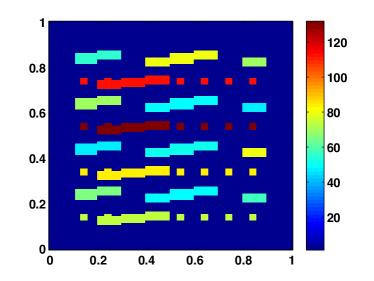
(a) Random field values

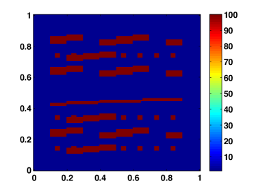
(b) Fixed field values

Figure 2: High-contrast permeability fields

To solve Eq. (23) we first linearize it by using a Picard iteration. In particular, for a given initial guess $u^{0}$ we solve

$$-\mbox{div}\big{(}\mathrm{e}^{\kappa(x)u^{n}(x)}\nabla u^{n+1}(x)\big{)} =f\,\,\,\text{in}\;D$$ (24a)

$$u^{n+1} =0\,\,\,\text{on}\;\partial D,$$ (24b)

for $n\geq 0$.

In our simulations, we take the initial guess $u^{0}=0$, and terminate the iterative loop when $\left\|A(u^{n+1})u^{n+1}-b\right\|\leq\delta\left\|b\right\|$, where $\delta$ is the tolerance for the iteration and we select $\delta=10^{-3}$. We note that $A$ and $b$ correspond to the linear system resulting from either the CG or DG global formulations. In particular, we solve the problem as follows:

$$A(u^{n})u^{n+1}=b\,\,\,\text{for}\,\,n=0,\,1,\ldots.$$ (25)

We note that since $u^{n}$ and $u^{n+1}$ will not necessarily be computed in coarse spaces of the same dimension, we cannot directly use the residual criterion listed above. Actually, we use the Galerkin projection of the fine solution to the corresponding coarse space to calculate the residual error from above.

Remark 1.

In this section we will consider two types of coefficients $\kappa(x)$ to be used in Eq. (23). We recall that throughout the paper we have used an auxiliary variable $\mu=\overline{u}^{n}$ to denote the solution dependence of the nonlinear problem. As such, we have referred to the model equation as parameter-dependent while describing the iterative solution procedure. Consequently, we are careful to introduce (and distinguish) a related case where we use a “physical” parameter $\mu^{\text{p}}$ for the purpose of constructing a field of the form $\kappa(x)=\mu^{\text{p}}\kappa_{1}(x)+(1-\mu^{\text{p}})\kappa_{2}(x)$. See Fig. 3 for an illustration of $\kappa_{1}(x)$ and $\kappa_{2}(x)$. We note that the coefficient will be constructed by summing contributions that depend on the physical parameter $\mu^{\text{p}}$, in addition to the auxiliary parameter dependence from the iterative form. In Subsect. 4.1 we use a field that does not depend on $\mu^{\text{p}}$, and in Subsect. 4.2 we use a field that does depend on $\mu^{\text{p}}$.

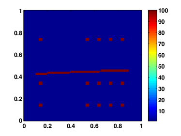
(a) $\kappa_{1}(x)$

(b) $\kappa_{2}(x)$

Figure 3: Decomposition of permeability field 2(b)

4.1 Parameter-independent permeability field

In the following simulations we first generate a snapshot space, use a spectral decomposition to obtain the offline space, and then for an initial guess apply a similar spectral decomposition to obtain the online space. We recall that in order to construct the snapshot space we choose a specified number of eigenfunctions (denoted by $M_{\text{snap}}$) on either a coarse neighborhood or coarse element depending on whether we use continuous (CG) or discontinuous Galerkin (DG) global coupling, respectively. In our simulations, we select the range of solutions $[u_{\text{min}},u_{\text{max}}]$ that correspond to solving the fine scale equation using a source term that ranges from $f\in[0.1,1]$. For the first set of simulations we divide the domain $[u_{\text{min}},u_{\text{max}}]$ into $N_{s}-1$ equally spaced subdomains to obtain $N_{s}$ discrete points $u_{1},\ldots,u_{N_{s}}$. For these simulations we fix a value of $N_{s}=9$.

For either formulation, we solve a localized eigenvalue problems as defined in Subsect. 3.1 for each point $u_{j}$ on a coarse neighborhood and keep a specified number of eigenfunctions. For example, in the CG case we keep $l_{\text{max}}=3$ snapshot eigenfunctions, and this construction leads to a local space of dimension $M_{\text{snap}}=l_{\text{max}}{\times}N_{s}=3{\times}9=27$. In the DG case, we adaptively choose the number of eigenfunctions based on a consideration of the eigenvalue differences. In the offline space construction we fix $\overline{u}$ as the average of the previously defined fixed snapshot values. We then solve the offline eigenvalue problem and construct the offline space by keeping the eigenvectors corresponding to a specified number of dominant eigenvalues. At the online stage we use the initial guess $u^{0}=0$ in order to solve the respective eigenvalue problem required for the space construction. We note that the size of our online space and the associated solution accuracy will depend on the number of eigenvectors that we keep in the online space construction.

In the CG formulation, we recall that the online eigenfunctions are multiplied by the corresponding partition of unity functions with support in the same neighborhood of the respective coarse node. We then solve Eq. (23) iteratively within the online space. In particular, for each iteration we update the online space and solve the equation Eq. (23) using the previously computed solution.

In the simulations using the CG formulation we discretize our domain into coarse elements of size $H=1/10$, and fine elements of size $h=1/100$. The results corresponding to the permeability fields from Figs. 2(a) and 2(b) are shown in Tables 1 and 2, respectively. The first column shows the dimension of the online solution space, and the second column shows the eigenvalue $\lambda^{*}$ which corresponds to the first eigenfunction that is discarded from space enrichment. We note that this eigenvalue is an important consideration in error estimates of enriched multiscale spaces ([22]). As a formal consideration, we mention that the error analysis typically yields estimates of the form $\|u-u_{\text{ms}}\|\sim\mathcal{O}(H^{\gamma}\lambda^{*})$ when the dominant eigenvalues are taken to be small. The next two columns correspond to the $L^{2}$-weighted relative error $\left\|u-u_{\text{ms}}\right\|_{L^{2}_{\kappa}(D)}/\left\|u\right\|_{L^{2}_{\kappa}(D)}{\times}100\%$ and energy relative error $\left\|u-u_{\text{ms}}\right\|_{H^{1}_{\kappa}(D)}/\left\|u\right\|_{H^{1}_{\kappa}(D)}{\times}100\%$ between the GMsFEM solution $u_{\text{ms}}$ and the fine-scale solution $u$. We note that as the dimension of the online space increases (i.e., we keep more eigenfunctions in the space construction), the relative errors decrease accordingly. As an example, for the field in Fig. 2(a), we encounter $L^{2}$ relative errors that decrease from $1.43-0.24\%$, and energy relative errors that decrease from $16.12-6.85\%$ as the online space is systematically enriched. In the tables, analogous errors between the online GMsFEM solution and the offline solution are computed. The dimension of the offline space is taken to be the maximum dimension of the online space. We note that in this case the Picard iteration converges in $4$ steps for all simulations. In Fig. 4 we also plot the fine and coarse-scale CG solutions that correspond to the field in Fig. 2(b). We note that the fine solution, and the coarse solutions corresponding to the largest and smallest online spaces are nearly indistinguishable.

We also illustrate the relation between the energy relative errors and $\lambda^{*}$ in Fig. 5 for the same permeability fields considered above. From the plots in Fig. 5, we see that the energy relative error predictably decreases as $\lambda^{*}$ decreases, thus following the appropriate error behavior.

$\dim(V_{\text{on}}^{\text{CG}})$	$\lambda^{*}$	GMsFEM Relative Error (%)		Online-Offline Relative Error (%)
		$L^{2}_{\kappa}(D)\hskip 17.07182pt$	$H^{1}_{\kappa}(D)$	$\hskip 17.07182ptL^{2}_{\kappa}(D)\hskip 17.07182pt$	$H^{1}_{\kappa}(D)$
$319$	$0.0021$	$1.43$	$16.12$	$1.25$	$16.33$
$497$	$0.0010$	$0.69$	$11.71$	$0.48$	$10.66$
$770$	$3.36\times 10^{-4}$	$0.40$	$9.13$	$0.20$	$7.30$
$1043$	$1.06\times 10^{-4}$	$0.31$	$7.76$	$0.09$	$4.43$
$1270$	—	$0.24$	$6.85$	0.00	0.00

Table 1: CG relative errors corresponding to the permeability field in Fig. 2(a)

$\dim(V_{\text{on}}^{\text{CG}})$	$\lambda^{*}$	GMsFEM Relative Error (%)		Online-Offline Relative Error (%)
		$L^{2}_{\kappa}(D)\hskip 17.07182pt$	$H^{1}_{\kappa}(D)$	$\hskip 17.07182ptL^{2}_{\kappa}(D)\hskip 17.07182pt$	$H^{1}_{\kappa}(D)$
$316$	$0.0026$	$1.36$	$15.28$	$1.18$	$15.74$
$482$	$0.0010$	$0.71$	$11.89$	$0.51$	$11.17$
$722$	$3.18\times 10^{-4}$	$0.43$	$9.53$	$0.22$	$7.77$
$996$	$1.02\times 10^{-4}$	$0.33$	$8.02$	$0.11$	$4.72$
$1236$	—	$0.26$	$7.05$	0.00	0.00

Table 2: CG relative errors corresponding to the permeability field in Fig. 2(b)

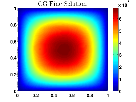
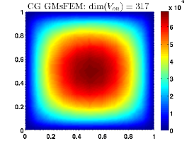
Figure 4: Comparison of fine and coarse CG solutions correpsonding to Fig. 2(b)

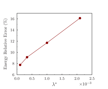
(a) Corresponds to Fig. 2(a)

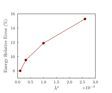
(b) Corresponds to Fig. 2(b)

Figure 5: Relation between the first discarded eigenvalue and the CG relative energy error; permeability from Fig. 2(a) (left), permeability from Fig. 2(b) (right)

In order to solve the model problem using the DG formulation, we note that the space of snapshots is constructed in a slightly different fashion. In this case, the selection of eigenvectors hinges on a comparison between the difference of consecutive eigenvalues resulting from the localized computations. In contrast to the CG case, the initial number of eigenfunctions (call this number $l_{\text{init}}^{K}$) used in the snapshot space construction are adaptively chosen based on the relative size of consecutive eigenvalues. For the results corresponding to the DG formulation, we note that two configurations for the snapshot space construction are used. In particular, we consider a case when the original number of eigenfuctions $l_{\text{init}}^{K}$ are used in the construction, and a case when $l_{\text{max}}^{K}=l_{\text{init}}^{K}+3$ are used in the construction.

In the simulations using the DG formulation, we partition the original domain using a coarse mesh of size $H=1/10$, and use a fine mesh composed of uniform triangular elements of mesh size $h=1/100$. The numerical results for permeability fields 2(a) and 2(b) are represented in Tables 3 and 4, respectively. The first column shows the dimension of the online space, the second column represents the corresponding eigenvalue($\lambda^{*}$) of the first eigenfunction discarded from the online space, and the next two columns illustrate the interior energy relative error ($E_{\text{int}}$) and the boundary energy relative error ($E_{\partial}$) between the fine scale solution and DG GMsFEM solution. The errors between the offline and online solutions are offered in the final two columns. We note that as the dimension of the online space increases (i.e., we keep more eigenfunctions in the space construction), the relative errors decrease accordingly. For example, the DG solution corresponding to Fig. 2(a) yields interior relative energy errors that decrease from $55.08-34.86\%$, and boundary relative energy errors that decrease from $8.94-6.40\%$. We note that in this case the Picard iteration converges in $4$ or $5$ steps for all simulations. In Fig. 6 we also plot the fine and coarse DG solutions that correspond to the field in Fig. 2(b). We note that the fine solution and the coarse solution corresponding to the smallest online space show some slight differences. However, the discrepancies noticeably diminish when the coarse DG solution is computed within the largest online space. As in the CG case, we also illustrate the relation between the DG interior errors and $\lambda^{*}$ in Fig. 7. From the plots in Fig. 7, we see that the relative errors decrease as $\lambda^{*}$ decreases, again following the expected error behavior.

$\dim(V_{\text{on}}^{\text{DG}})$	$\lambda^{*}$	GMsFEM Relative Error (%)		Online-Offline Relative Error (%)
		$\hskip 17.07182ptE_{\text{int}}\hskip 17.07182pt$	$E_{\partial}$	$\hskip 22.76228ptE_{\text{int}}\hskip 22.76228pt$	$E_{\partial}$
$271$	$1.53\times 10^{-4}$	$55.08$	$8.94$	$44.38$	$8.43$
$331$	$1.24\times 10^{-4}$	$36.59$	$6.63$	$10.05$	$3.08$
$466$	$3.03\times 10^{-5}$	$35.57$	$6.56$	$7.00$	$1.67$
$624$	$1.72\times 10^{-5}$	$34.90$	$6.48$	$2.12$	$0.40$
$716$	—	$34.86$	$6.40$	0.00	0.00

Table 3: DG relative errors corresponding to the permeability field in Fig. 2(a); snapshot space uses $l_{\text{init}}^{K}$ eigenfunctions

$\dim(V_{\text{on}}^{\text{DG}})$	$\lambda^{*}$	GMsFEM Relative Error (%)		Online-Offline Relative Error (%)
		$\hskip 17.07182ptE_{\text{int}}\hskip 17.07182pt$	$E_{\partial}$	$\hskip 19.91684ptE_{\text{int}}\hskip 19.91684pt$	$E_{\partial}$
$270$	$1.56\times 10^{-4}$	$56.29$	$10.30$	$46.37$	$9.75$
$331$	$1.05\times 10^{-4}$	$36.72$	$6.71$	$9.54$	$3.32$
$444$	$3.12\times 10^{-5}$	$35.67$	$6.56$	$6.48$	$1.67$
$582$	$1.21\times 10^{-5}$	$35.06$	$6.48$	$2.14$	$0.41$
$663$	—	$35.03$	$6.48$	0.00	0.00

Table 4: DG relative errors corresponding to the permeability field in Fig. 2(b); snapshot space uses $l_{\text{init}}^{K}$ eigenfunctions

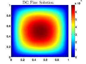
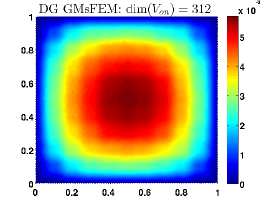
Figure 6: Comparison of fine and coarse DG solutions correpsonding to Fig. 2(b)

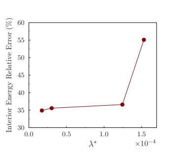
(a) Corresponds to Fig. 2(a)

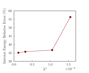
(b) Corresponds to Fig. 2(b)

Figure 7: Relation between the first discarded eigenvalue and the DG relative interior energy error; permeability from Fig. 2(a) (left), permeability from Fig. 2(b) (right) 2(a) and 2(b)

Remark 2.

When solving the nonlinear equation using the discontinuous Galerkin approach, we use different penalty parameters for fine-grid problem and coarse-grid problem (refer back to Subsect. 3.2.2). However, we observe that for different coarse penalty parameters that yield a convergent solution, the number of iterations and the relative errors (both interior and boundary) stay the same.

Remark 3.

Recall that we use the Galerkin projection of the previous coarse solution onto the current online space as the approximation of the previous coarse solution to obtain the terminal condition. If the coarse penalty parameter is changed, we should use the current coarse penalty parameter to construct the Galerkin projection.

We observe from Tables 1-4 that the offline spaces for DG formulation are much smaller than those obtained through CG formulation. As a result, in Table 5 we use more eigenfunctions (more specifically, we set $l_{\text{max}}^{K}=l_{\text{init}}^{K}+3$) in the snapshot space construction to yield a larger offline space. For these examples, we use the permeability field from Fig. 2(b). Due to the increase of the offline (and corresponding online) space dimensions, we see more accurate results than those offered in Table 4.

$\dim(V_{\text{on}}^{\text{DG}})$	$\lambda^{*}$	GMsFEM Relative Error (%)		Online-Offline Relative Error (%)
		$\hskip 17.07182ptE_{\text{int}}\hskip 17.07182pt$	$E_{\partial}$	$\hskip 22.76228ptE_{\text{int}}\hskip 22.76228pt$	$E_{\partial}$
$381$	$1.47\times 10^{-4}$	$37.34$	$7.42$	$22.80$	$6.00$
$440$	$1.54\times 10^{-4}$	$35.92$	$6.16$	$20.07$	$4.36$
$707$	$9.54\times 10^{-5}$	$32.80$	$5.29$	$13.64$	$2.90$
$958$	$2.71\times 10^{-5}$	$29.44$	$5.48$	$4.80$	$0.98$
$1352$	—	$28.98$	$5.39$	0.00	0.00

Table 5: DG relative errors corresponding to the permeability field in Fig.2(b); snapshot space uses $l_{\text{max}}^{K}=l_{\text{init}}^{K}+3$ eigenfunctions

4.2 Parameter-dependent permeability field

For the next set of numerical results, we consider solving the nonlinear elliptic problem in Eq. (23) with a coefficient of the form $\kappa(x,u,\mu^{\text{p}})=\exp\left[\left(\mu^{\text{p}}\kappa_{1}(x)+(1-\mu^{\text{p}})\kappa_{2}(x)\right)u(x)\right]$. For $\kappa_{1}(x)$ and $\kappa_{2}(x)$ we use the fields shown in Fig. 3(a) and 3(b), respectively. As for the parameter-dependent simulation, we are careful to distinguish the difference between the auxiliary parameter $\mu=\overline{u}^{n}$ which is used to denote a previous solution iterate, and a “physical” parameter $\mu^{\text{p}}$ that is used in the construction of a new permeability field. We take the range of $\mu^{\text{p}}$ to be $[0,1]$, and use three equally spaced values in order to construct the snapshot space in this case. We use the same $[u_{\text{min}},u_{\text{max}}]$ interval from the previous results, yet use four equally spaced values in this case. In particular, we use the pairs $(u_{j},\mu_{l}^{\text{p}})$, where $1\leq j\leq 4$, and $1\leq l\leq 3$ as the fixed parameter values for the snapshot space construction. At the online stage we use the initial guess $u^{0}=0$ and a fixed value of $\mu^{\text{p}}=0.2$ while solving the respective eigenvalue problem required for the continuous or discontinuous Galerkin online space construction.

In Table 6 we offer results corresponding to the CG formulation, and in Tables 7 and 8 we offer results corresponding to the DG formulation. In all cases we encounter very similar error behavior compared to the examples offered earlier in the section. In particular, an increase of the dimension of the online space yields predictably smaller errors, and smaller values of $\lambda^{*}$ correspond to the error decrease. And while it suffices to refer back to related discussions earlier in the section, we emphasize that this distinct set of results serves to further illustrate the robustness of the proposed method. In particular, we show that the solution procedure allows for a suitable treatment of nonlinear problems that involve auxiliary and physical parameters.

$\dim(V_{\text{on}}^{\text{CG}})$	$\lambda^{*}$	GMsFEM Relative Error (%)		Online-Offline Relative Error (%)
		$L^{2}_{\kappa}(D)\hskip 17.07182pt$	$H^{1}_{\kappa}(D)$	$\hskip 17.07182ptL^{2}_{\kappa}(D)\hskip 17.07182pt$	$H^{1}_{\kappa}(D)$
$309$	$0.0027$	$1.30$	$14.89$	$1.10$	$15.32$
$492$	$0.0010$	$0.59$	$10.82$	$0.39$	$9.76$
$580$	$6.76\times 10^{-4}$	$0.45$	$9.55$	$0.24$	$7.92$
$728$	$3.33\times 10^{-4}$	$0.34$	$7.87$	$0.12$	$5.23$
$991$	—	$0.28$	$6.74$	0.00	0.00

Table 6: CG relative errors corresponding to the parameter-dependent field constructed from Fig. 3(a) and 3(b)

$\dim(V_{\text{on}}^{\text{DG}})$	$\lambda^{*}$	GMsFEM Relative Error (%)		Online-Offline Relative Error (%)
		$\hskip 17.07182ptE_{\text{int}}\hskip 17.07182pt$	$E_{\partial}$	$\hskip 22.76228ptE_{\text{int}}\hskip 22.76228pt$	$E_{\partial}$
$300$	$1.02\times 10^{-4}$	$37.56$	$7.94$	$10.15$	$3.16$
$313$	$6.25\times 10^{-5}$	$37.55$	$7.81$	$10.00$	$2.85$
$403$	$2.58\times 10^{-5}$	$36.81$	$7.35$	$5.83$	$1.38$
$497$	$1.22\times 10^{-5}$	$36.37$	$7.21$	$0.84$	$0.10$
$517$	—	$36.36$	$7.21$	0.00	0.00

Table 7: DG relative errors corresponding to the parameter-dependent field constructed from Fig. 3(a) and 3(b); snapshot space uses $l_{\text{init}}^{K}$ eigenfunctions

$\dim(V_{\text{on}}^{\text{DG}})$	$\lambda^{*}$	GMsFEM Relative Error (%)		Online-Offline Relative Error (%)
		$\hskip 17.07182ptE_{\text{int}}\hskip 17.07182pt$	$E_{\partial}$	$\hskip 22.76228ptE_{\text{int}}\hskip 22.76228pt$	$E_{\partial}$
$300$	$2.13\times 10^{-4}$	$37.59$	$7.94$	$22.54$	$6.40$
$440$	$1.54\times 10^{-5}$	$35.78$	$5.92$	$18.89$	$3.74$
$668$	$7.69\times 10^{-5}$	$32.54$	$5.39$	$11.62$	$2.58$
$902$	$1.51\times 10^{-5}$	$30.23$	$5.29$	$3.87$	$1.06$
$1093$	—	$29.88$	$5.29$	0.00	0.00

Table 8: DG relative errors corresponding to the parameter-dependent field constructed from Fig. 3(a) and 3(b); snapshot space uses $l_{\text{max}}^{K}=l_{\text{init}}^{K}+3$ eigenfunctions

5 Concluding Remarks

In this paper we use the Generalized Multiscale Finite Element (GMsFEM) framework in order to solve nonlinear elliptic equations with high-contrast coefficients. In order to solve this type of problem we linearize the equation such that upscaled quantities of previous solution iterates may be regarded as auxiliary coefficient parameters in the problem formulation. As a result, we are able to construct a respective set of coarse basis functions using an offline-online procedure in which the precomputed offline space allows for the efficient computation of a smaller-dimensional online space for any parameter value at each iteration. In this paper, the coarse space construction involves solving a set of localized eigenvalue problems that are tailored to either continuous Galerkin (CG) or discontinuous Galerkin (DG) global coupling mechanisms. In particular, the respective coarse spaces are formed by keeping a set of eigenfunctions that correspond to the localized eigenvalue behavior. Using either formulation, we show that the process of systematically enriching the coarse solution spaces yields a predictable error decline between the fine and coarse-grid solutions. As a result, the proposed methodology is shown to be an effective and flexible approach for solving the nonlinear, high-contrast elliptic equation that we consider in this paper.

References

References

- [1] J. E. Aarnes, On the use of a mixed multiscale finite element method for greater flexibility and increased speed or improved accuracy in reservoir simulation, SIAM J. Multiscale Modeling and Simulation, 2 (2004), 421-439.
- [2] J. E. Aarnes, S. Krogstad, and K.-A. Lie, A hierarchical multiscale method for two-phase flow based upon mixed finite elements and nonuniform grids, Multiscale Model. Simul. 5(2) (2006), pp. 337–363.
- [3] T. Arbogast, G. Pencheva, M. F. Wheeler, and I. Yotov, A multiscale mortar mixed finite element method, SIAM J. Multiscale Modeling and Simulation, 6(1), 2007, 319-346.
- [4] D. N. Arnold, F. Brezzi, B. Cockburn, and L. D. Marini, Unified analysis of discontinuous Galerkin methods for elliptic problems, SIAM J. Numer. Anal., 39 (2001/02), pp. 1749–1779 (electronic).
- [5] I. Babuska and R. Lipton, Optimal Local Approximation Spaces for Generalized Finite Element Methods with Application to Multiscale Problems. Multiscale Modeling and Simulation, SIAM 9 (2011) 373-406
- [6] I. Babuška and J. M. Melenk, The partition of unity method, Internat. J. Numer. Methods Engrg., 40 (1997), pp. 727-758.
- [7] I. Babuška and E. Osborn, Generalized Finite Element Methods: Their Performance and Their Relation to Mixed Methods, SIAM J. Numer. Anal., 20 (1983), pp. 510-536.
- [8] M. Barrault, Y. Maday, N.C. Nguyen, and A.T. Patera, An ’Empirical Interpolation’ Method: Application to Efficient Reduced-Basis Discretization of Partial Differential Equations. CR Acad Sci Paris Series I 339:667-672, 2004.
- [9] L. Berlyand and H. Owhadi, Flux norm approach to finite dimensional homogenization approximations with non-separated scales and high contrast, Arch. Ration. Mech. Anal., 198 (2010), pp. 677-721.
- [10] S. Boyoval, Reduced-basis approach for homogenization beyond periodic setting, SIAM MMS, 7(1), 466-494, 2008.
- [11] S. Boyaval, C. LeBris, T. Lelièvre, Y. Maday, N. Nguyen, and A. Patera, Reduced Basis Techniques for Stochastic Problems, Archives of Computational Methods in Engineering, 17:435-454, 2010.
- [12] Y. Chen and L. Durlofsky, An ensemble level upscaling approach for efficient estimation of fine-scale production statistics using coarse-scale simulations, SPE paper 106086, presented at the SPE Reservoir Simulation Symposium, Houston, Feb. 26-28 (2007).
- [13] Y. Chen, L.J. Durlofsky, M. Gerritsen, and X.H. Wen, A coupled local-global upscaling approach for simulating flow in highly heterogeneous formations, Advances in Water Resources, 26 (2003), pp. 1041–1060.
- [14] J. Douglas, Jr, P. J. Pacs-Leme and T. Giorgi, Generalized Forchheimer Flow in Porous Media, in Boundary Value Problems for Partial Differential Equations and Applications, RMA Res. Notes, Appl.Math.,29, Masson, Paris, 1993, pp.99-103.
- [15] M. Dryja, On discontinuous Galerkin methods for elliptic problems with discontinuous coefficients, Comput. Methods Appl. Math., 3 (2003), pp. 76–85 (electronic).
- [16] Y. Efendiev, J. Galvis, S. Ki Kang, and R.D. Lazarov. Robust multiscale iterative solvers for nonlinear flows in highly heterogeneous media. Numer. Math. Theory Methods Appl., 5(3):359 1 73, 2012.
- [17] Y. Efendiev, J. Galvis and P. Vassielvski, Spectral element agglomerate algebraic multigrid methods for elliptic problems with high-Contrast coefficients, in Domain Decomposition Methods in Science and Engineering XIX, Huang, Y.; Kornhuber, R.; Widlund, O.; Xu, J. (Eds.), Volume 78 of Lecture Notes in Computational Science and Engineering, Springer-Verlag, 2011, Part 3, 407-414.
- [18] Y. Efendiev, J. Galvis, R. Lazarov, M. Moon, M. Sarkis, Generalized Multiscale Finite Element Method. Symmetric Interior Penalty Coupling, In preparation.
- [19] Y. Efendiev, J. Galvis, R. Lazarov, and J. Willems, Robust domain decomposition preconditioners for abstract symmetric positive definite bilinear forms, submitted.
- [20] Y. Efendiev, J. Galvis, and T. Hou, Generalized Multiscale Finite Element Methods, submitted. http://arxiv.org/submit/631572
- [21] Y. Efendiev, J. Galvis, and F. Thomines, A systematic coarse-scale model reduction technique for parameter-dependent flows in highly heterogeneous media and its applications, 2011
- [22] Y. Efendiev, J. Galvis, and X. H. Wu, Multiscale finite element methods for high-contrast problems using local spectral basis functions, Journal of Computational Physics. Volume 230, Issue 4, 20 February 2011, Pages 937-955.
- [23] Y. Efendiev, V. Ginting, T. Hou, and R. Ewing, Accurate multiscale finite element methods for two-phase flow simulations, J. Comp. Physics, 220 (1), pp. 155–174, 2006.
- [24] Y. Efendiev and T. Hou, Multiscale finite element methods. Theory and applications, Springer, 2009.
- [25] Y. Efendiev, T. Hou, and V. Ginting. Multiscale finite element methods for nonlinear problems and their applications. Comm. Math. Sci., 2:553 1 79, 2004.
- [26] J. Galvis and Y. Efendiev, Domain decomposition preconditioners for multiscale flows in high-contrast media: Reduced dimension coarse spaces, SIAM J. Multiscale Modeling and Simulation, Volume 8, Issue 5, 1621-1644 (2010).
- [27] R. C. Givler and S. A. Altobelli, A determination of the effective viscosity for the Brinkman Forchheimer flow model, Journal of Fluid Mechanics, Volume 258, pp 355-370(1994).
- [28] T.Y. Hou and X.H. Wu, A multiscale finite element method for elliptic problems in composite materials and porous media, Journal of Computational Physics, 134 (1997), 169-189.
- [29] T. Hughes, G. Feijoo, L. Mazzei, and J. Quincy, The variational multiscale method - a paradigm for computational mechanics, Comput. Methods Appl. Mech. Engrg, 166 (1998), 3-24.
- [30] P. Jenny, S.H. Lee, and H. Tchelepi, Multi-scale finite volume method for elliptic problems in subsurface flow simulation, J. Comput. Phys., 187 (2003), 47-67.
- [31] L. Machiels, Y. Maday, I.B. Oliveira, A.T. Patera, and D.V. Rovas, Output bounds for reduced-basis approximations of symmetric positive definite eigenvalue problems, Comptes Rendus de l’Académie des Sciences, 331(2):153-158, 2000.
- [32] Y. Maday, Reduced-basis method for the rapid and reliable solution of partial differential equations. In: Proceedings of international conference of mathematicians, Madrid. European Mathematical Society, Zurich, 2006.
- [33] M.A. Grepl, Y. Maday, N.C. Nguyen, and A.T. Patera. Efficient reduced-basis treatment of non-affine and nonlinear partial differential equations. ESIAM : M2AN, 41(2):575 1 75, 2007.
- [34] N. C. Nguyen, A multiscale reduced-basis method for parameterized elliptic partial differential equations with multiple scales, J. Comp. Physics, 227(23), 9807-9822, 2008.
- [35] L. Richards, Capillary conduction of liquids through porous mediums, Physics, pp. 318-333, 1931.
- [36] B. Rivière, Discontinuous Galerkin methods for solving elliptic and parabolic equation, vol. 35 of Frontiers in Applied Mathematics, Society for Industrial and Applied Mathematics (SIAM), Philadelphia, 2008.
- [37] G. Rozza, D. B. P Huynh, and A. T. Patera, Reduced basis approximation and a posteriori error estimation for affinely parametrized elliptic coercive partial differential equations. Application to transport and continuum mechanics. Arch Comput Methods Eng 15(3):229?275, 2008.