The magnetization plateaus of the ferro and anti-ferro spin-1 classical models with $S_{z}^{2}$ term

Abstract

We study in detail the exact thermodynamics of the one-dimensional standard and staggered spin-1 Ising models with a single-ion anisotropy term in the presence of a longitudinal magnetic field at low temperatures. The results are valid for the ferromagnetic and anti-ferromagnetic (AF) models and for positive and negative values of the crystal field for $T>0$. Although the excited states of the ferro and anti-ferro models are highly degenerate, we show that the temperature required for reaching the first excited state in the classical spin-1 ferro model gives a scale of temperature that permits fitting the $z$-component of the magnetization only by the contribution of two ground states of the model. This approximation is not true for the equivalent AF function due to the fact that the AF model is gapless along the lines separating the phases in its phase diagram at $T=0$. We relate the number of plateaus in the magnetization of each model to their respective phase diagrams at $T=0$. The specific heat per site of the AF model distinguishes, at low temperature, the transitions $\mbox{A}\rightleftharpoons\mbox{E}$ and $\mbox{G}\rightleftharpoons\mbox{E}$ as the external magnetic field is varied. The exact Helmholtz free energy of the classical spin-1 model is mapped onto the equivalent function of the ionic limit of the $1D$ extended Hubbard model by proper transformations.

Keywords: Quantum statistical mechanics, Ising model, spin-1, single-ion anisotropy term, staggered, thermodynamics, optical device.

PACS numbers: 05.30.-d, 75.10.Hk, 75.10.Jm

1 Introduction

Exactly solvable models help us having insights on more complex systems. In one space dimension ($1D$), the thermodynamics of the spin-$\frac{1}{2}$ Ising model in the presence of a longitudinal magnetic field has been solved in the whole interval of temperature using the density matrix approach[1, 2, 3]. To do so, it is essential the commutative nature of all operators in its Hamiltonian. This model is usually called a classical system.

Cold atoms have made possible simulations of spin models. Recently Simon et al.[4] simulated a one-dimensional spin-$1/2$ model in the presence of a magnetic field with longitudinal and transverse components by using a Mott insulator of spinless bosons in a tilted optical lattice. The device was used to study the phases of this classical model at low temperatures. These optical devices have permitted the experimental study of properties of chain models, including the spin models.

The spin-1 Ising model with single-ion anisotropy term, the Blume[5]-Capel[6] model, in the presence of a longitudinal magnetic field, has also a classical nature. This fact permits us to apply the transfer matrix method[1, 2, 3] to solve it. With this approach, Aydiner and Akyüz [7] obtained the numerical solution of the $1D$ spin-1 anti-ferromagnetic (AF) Ising model with a single-ion anisotropy term in the presence of a longitudinal magnetic field. They studied the magnetic and thermal behavior of the model at very low temperatures. In 2003 Chen et al.[8] applied the classical Monte Carlo (CMC) technique to the numerical calculation of the phase diagram at $T=0$ of the spin-$1$ anti-ferromagnetic Ising model in the presence of a single-ion anisotropy term for positive crystal field. The CMC was applied also to the study of magnetization plateaus of this model at low temperature.

In 2005 Mancini[9] used the mapping between the $1D$ extended Hubbard model in the ionic limit (i.e., $|t|\ll|U|,|V|$, in which $t$ is the hopping exchange, $U$ is the on-site Coulomb interactions and $V$ is the inter-site Coulomb interaction) and the spin-1 Ising model with a single-ion anisotropy term in the presence of a longitudinal magnetic field to write the exact Helmholtz free energy (HFE) of the latter[9] as a set of coupled equations. The hierarchy of the equations of motion is closed, and they can be solved numerically. In Ref.[10] they have extended the approach to include a biquadratic nearest-neighbour interaction term, numerically solving the coupled equations and presenting the behavior of some thermodynamic functions at low temperatures. We derived in Ref.[11] the exact expression of the HFE of the $1D$ spin-1 Ising model with the $(S_{z})^{2}$ term in the absence of a magnetic field. This HFE has a simple analytic expression valid for the ferromagnetic and AF models in the whole range of temperature. The absence of a magnetic field in this solution prevents accessing some information about the system, e.g.: information about the magnetization and the susceptibility of the model.

All the previously mentioned papers on the one-dimensional spin-1 Ising model seem to be unaware of the nice work by Krinsky and Furman[12] in 1976, which presents the calculation of the exact HFE for the $1D$ ferromagnetic spin-1 Ising model with a single-ion anisotropy term, a biquadratic nearest-neighbour interaction term and a nonsymmetric term, in the presence of a longitudinal magnetic field. More recently Litaiff et al. also applied the transfer-matrix technique to calculate the exact expression of the HFE of this model. The authors did not use this thermodynamic function to explore its low temperature behavior.

Although the $1D$ spin-$S$ Ising model with the single-ion anisotropy term in the presence of a magnetic field is called a classical model, it has a quantum nature that manifests itself as plateaus in the $z$-component of the magnetization at very low temperature. The existence of those plateaus has been demonstrated in a number of $1D$ models[14] and experimentally measured in some materials[15, 16, 17] described by $1D$ spin-models. Magnetization plateaus in the the AF spin-1 Ising model with positive crystal field in the presence of a longitudinal magnetic field have been obtained numerically in Refs.[7, 8, 10]. The authors of Ref.[12] mentioned the discontinuous change of the magnetization of the ferromagnetic model, but their focus was on the exact renormalization group of the model and the discussion of its critical points.

The study of the simple one-dimensional spin-1 Ising model helps to understand the origin of plateaus in the magnetization function. In the present communication we present the exact analytic expressions of the HFE’s of the standard and the staggered versions of the $1D$ spin-1 Ising model with the $(S_{i}^{z})^{2}$ term in the presence of a longitudinal magnetic field, valid for $T>0$ in section 2. Our solutions apply equally well to the ferromagnetic and to the AF models of both versions, extending the validity of the solution derived in Ref.[12] for the ferromagnetic model. We study the $z$-component of the magnetization and the entropy per site at very low temperatures for the ferro and AF versions of the classical spin-1 model in sections 3 and 4, respectively. We relate the number of plateaus in the magnetization to the number of phases in the ground state of the model at $T=0$. Finally in section 5 we present our conclusions. More detailed calculations are shown in Appendices A and B.

2 The Hamiltonians of the classical spin-1 models in the presence of a longitudinal magnetic field

The Hamiltonian of the one-dimensional of the classical spin-1 Ising model with a single-ion anisotropy term, the Blume-Capel model, in the presence of a longitudinal magnetic field is[5, 6]

$${\mathbf{H}}^{\prime} = \overset{N}{\underset{i=1}{\sum}}\;\;\left[JS_{i}^{z}S_{i+1}^{z}-h^{\prime}S_{i}^{z}+D^{\prime}(S_{i}^{z})^{2}\right]$$ (1)

$$= \overset{N}{\underset{i=1}{\sum}}\;\;{\bf H}_{i,i+1},$$

where $S_{i}^{z}$ is the $z$- component of the spin-1 operator with norm: $||\vec{S}||^{2}=2$. $J$ is the exchange strength and it can have either a negative value (ferromagnetic model) or a positive value (AF model). The crystal field $D$ can assume positive, negative or null values. The model satisfies spacial periodic boundary condition in a chain with $N$ sites. The external magnetic field is oriented along the easy-axis $z$. In this paper we use natural units, $e=m=\hbar=1$. Comparing our Hamiltonian (1) to the Hamiltonian (25) in Ref.[13] we have $J=J^{*}$, $h^{\prime}=\mu_{B}H^{*}$ and $D^{\prime}=D^{*}$, in which $J^{*}$, $H^{*}$ and $D^{*}$ are the parameters of the Hamiltonian of the single spin-1 Ising model in Ref.[13].

Mancini[9] showed that by the substitution $S_{i}^{z}={\mathbf{n}}_{i}-{\mathbf{1}}_{i}$ (where ${\mathbf{1}}_{i}$ is the identity operator at the $i$-th site, in which ${\mathbf{n}}_{i}={\mathbf{n}}_{i,\uparrow}+{\mathbf{n}}_{i,\downarrow}$,   ${\mathbf{n}}_{i,\sigma}\equiv{\mathbf{c}}_{i,\sigma}^{{\dagger}}{\mathbf{c}}_{i,\sigma}$ with $\sigma\in\{\uparrow,\downarrow\}$, ${\mathbf{c}}_{i,\sigma}^{{\dagger}}$ is the fermionic creation operator of an electron at the $i$-th site with the spin component $\sigma$ and ${\mathbf{c}}_{i,\sigma}$ is the corresponding destruction operator, the Hamiltonian (1) is mapped onto the ionic limit of the Hamiltonian of the 1D extended Hubbard model in the presence of a chemical potential, that is

$${\mathbf{H}}^{\prime}={\mathbf{H}}_{Hub}+N(J+h^{\prime}+D^{\prime})\;{\mathbf{1}},$$ (2)

where[18, 19]

$${\mathbf{H}}_{Hub}=\sum_{i=1}^{N}\;\;\left(U{\mathbf{n}}_{i,\uparrow}{\mathbf{n}}_{i,\downarrow}+2V{\mathbf{n}}_{i}\,{\mathbf{n}}_{i+1}-\mu{\mathbf{n}}_{i}\right).$$ (3)

The last equality is valid for $U=2D^{\prime}$, $V=\frac{J}{2}$ and $\mu=2J+h^{\prime}+D^{\prime}$. As a consequence of relation (2) we have, for these values of parameters, that ${\mathcal{W}}_{Hub}(U,V,\mu;\beta)={\mathcal{W}}_{1}(J,h^{\prime},D^{\prime};\beta)-(J+h^{\prime}+D^{\prime})$, where ${\mathcal{W}}_{Hub}$ (${\mathcal{W}}_{1}$) is the HFE of the extended Hubbard model in the ionic limit (the HFE of the spin-1 Ising model (1)). One is reminded that $\beta=\frac{1}{kT}$, where $k$ is the Boltzmann’s constant and $T$ is the absolute temperature in kelvin.

The Hamiltonian (1) in the presence of a staggered longitudinal magnetic field is

$${\mathbf{H}}_{stag}^{\prime} = \overset{2M}{\underset{i=1}{\sum}}\;\;\left[JS_{i}^{z}S_{i+1}^{z}-h^{\prime}\;(-1)^{i}\;S_{i}^{z}+D^{\prime}(S_{i}^{z})^{2}\right].$$ (4)

The Hamiltonian continues to satisfy space periodic condition, but now we have an even number of sites in the chain: $N=2M$.

Applying the method presented in Ref.[20] we calculated in Ref.[21] the $\beta$-expansion of the HFE of the one-dimensional spin-$S$ Ising model, with single-ion anisotropy term, in the presence of a longitudinal magnetic field, ${\mathcal{W}}_{S}(J,h^{\prime},D^{\prime};\beta)$, up to order $\beta^{17}$, in the thermodynamic limit. The $\beta$-expansion of the HFE of the staggered Hamiltonian (4), with $D^{\prime}=0$, ${\mathcal{W}}_{S}^{stag}(J,h^{\prime},0;\beta)$, was derived in Ref.[22] up to the same order in $\beta$ also for $M\rightarrow\infty$. Unfortunately those expansions do not permit us to study the thermodynamics of the standard and the staggered $1D$ spin-1 Ising model close to $T=0$. In our web page we provide the data files with the quantum (arbitrary spin-$S$) and the classical HFE’s of the normalized Hamiltonians (1) and (4) up to order $\beta^{17}$ for both versions (standard and staggered) of the model.

In the present work we apply the transfer matrix method[3] together with the $\beta$-expansion of the function ${\mathcal{W}}_{1}(J,h^{\prime},D^{\prime};\beta)$ obtained from the results of Ref.[21] with $S=1$ to calculate the exact HFE of the Hamiltonian (1) in the thermodynamic limit ($N\rightarrow\infty$), valid for $T\stackrel{{\scriptstyle>}}{{{}_{\sim}}}0$. The expression of ${\mathcal{W}}_{1}^{stag}(J,h^{\prime},D^{\prime};\beta)$ is obtained by using a well known result in the literature[22], namely, ${\mathcal{W}}_{S}^{stag}(J,h^{\prime},D^{\prime};\beta)={\mathcal{W}}_{S}(-J,h^{\prime},D^{\prime};\beta)$, with $S=\frac{1}{2},1,\frac{3}{2},\cdots$. This equality is valid for $T\in[0,\infty)$.

In order to calculate the exact function ${\mathcal{W}}_{1}(J,h^{\prime},D^{\prime};\beta)$, valid for $T>0$ and in the limit of $N\rightarrow\infty$, using the transfer matrix method, we rewrite Hamiltonian (1) as a symmetric operator in the $i$-th and $(i+1)$-th sites, that is,

$${\bf H}_{i,i+1}^{(S)}=JS_{i}^{z}S_{i+1}^{z}-hS_{i}^{z}-hS_{i+1}^{z}+D(S_{i}^{z})^{2}+D(S_{i+1}^{z})^{2}.$$ (5)

By comparing eqs.(1) and (5), we verify that the $\beta$-expansion of the HFE of this model, in terms of the parameters $J$, $h$ and $D$ in Hamiltonian (5) may be obtained by applying the following change of variables: $h^{\prime}\rightarrow 2h$ and $D^{\prime}\rightarrow 2D$, in the expansion of Ref.[21] with $S=1$.

In appendix A we calculate the three roots of the third degree equation derived from the transfer matrix method for the classical spin-1 model with a single-ion anisotropy term in the presence of a longitudinal magnetic field. The root with the largest modulus gives the expression of the HFE of the model (1)/(5) (see eq. (A.7)).

In order to verify which root, eqs.(A.11a) - (A.11c), corresponds to the eigenvalue $\lambda_{1}$ of matrix U, assumed to be the root with the largest modulus, we calculate the $\beta$-expansion of the functions $-\frac{1}{\beta}\ln[s_{i}]$, $i=1,2,3$, and compare each one with the expansion of the HFE of Ref.[21] with $S=1$ (having made the change of variables $h^{\prime}=2h$ and $D^{\prime}=2D$ in the $\beta$-expansion of Ref.[21]). By direct comparison of the expansions, we obtain for finite value of $\beta$, up to order $\beta^{10}$, that the root $s_{1}$, eq.(A.11a), is the eigenvalue $\lambda_{1}$, that has the largest modulus among the eigenvalues of matrix U. Our analysis is valid for finite value of $\beta$, which excludes the value $T=0$.

Our solution $s_{1}$ is equal to the eigenvalue of the cubic equation with the largest modulus calculated in Ref.[12] for the ferromagnetic model ($J<0$). The way we write the solutions (A.12a) - (A.12c) avoids the necessity of defining a cut in the complex plane for their calculation. Our results extended those derived in Ref.[12] to include the HFE of the AF spin-1 Ising model in the presence of a longitudinal magnetic field.

The exact HFE of the standard one-dimensional spin-1 Ising model with the single-ion anisotropy term in the presence of a longitudinal magnetic field $h$ is

$${\mathcal{W}}_{1}(J,h,D;\beta)=-\frac{1}{\beta}\;\;\ln\left[2\sqrt{-\tilde{Q}}\;\;\cos(\frac{\theta}{3})+\frac{P}{3}\right],$$ (6)

in which $P$, $\theta$ and $\tilde{Q}$ are given respectively by eqs.(A.10a), (A.12a), (A.12b). The HFE (6) is an even function of $h$: ${\mathcal{W}}_{1}(J,h,D;\beta)={\mathcal{W}}_{1}(J,-h,D;\beta)$. One is reminded that ${\mathcal{W}}_{1}^{stag}(J,h^{\prime},D^{\prime};\beta)={\mathcal{W}}_{1}(-J,h^{\prime},D^{\prime};\beta)$ and ${\mathcal{W}}_{Hub}(U,V,\mu;\beta)={\mathcal{W}}_{1}(J,h^{\prime},D^{\prime};\beta)-(J+h^{\prime}+D^{\prime})$, with $U=2D^{\prime}$, $V=\frac{J}{2}$ and $\mu=2J+h^{\prime}+D^{\prime}$.

From the simple expression (6) one can calculate the thermodynamic functions of the standard and the staggered models, as well of the extended Hubbard model in the ionic limit in the absence of an external magnetic field, for any finite value of $\beta$, that does not include the temperature $T=0$, that is, $T\in(0,\infty)$. It is a well known fact that at $T=0$, $h=0$ and $D=0$, two eigenvalues of matrix U are degenerated. Our results are valid in the limit of $T\rightarrow 0$. Due to the presence of the longitudinal magnetic field in the HFE (6) we can derive from it the $z$-component of the magnetization and the magnetic susceptibility per site for the ferromagnetic ($J<0$) and AF ($J>0$) versions of the standard Hamiltonian (1)/ (5) as well as the staggered magnetization and the staggered magnetic susceptibility[22] of the Hamiltonian (4) for any value of the exchange strength $J$. For $h=0$, the expression (6) of the HFE ${\mathcal{W}}_{1}(J,0,D;\beta)$ coincides with the exact result presented in Ref.[11].

Our exact result permits us to study the plateaus of the standard and the staggered $z$ component of the magnetization per site of the ferro and the AF models of the standard and the staggered versions, respectively, of the one-dimensional spin-1 Ising model, with the single-ion anisotropy term, in the presence of a longitudinal magnetic field for temperatures close to $T\sim 0$. The authors of Ref.[12] mentioned the discontinuity of the magnetization and the magnetic quadrupolar moment of the ferromagnetic model at $T=0$, not going any further on this point. Aydiner and Akyüz [7] and Chen et al [8] studied numerically these plateaus in the AF version of Hamiltonian (1)/(5). More recently, Mancini and Mancini[10] solved (also numerically) the self consistent equations that yield the exact HFE of the AF $S=1$ Ising model with a biquadratic nearest-neighbour term in the presence of a longitudinal magnetic field.

In the rest of this paper we let $J=-1$ for the ferromagnetic model and $J=1$ for the AF model. The values of the parameters $D$, $h$ and $T$ are given in units of $|J|$, that is: $\frac{D}{|J|}$, $\frac{h}{|J|}$ and $\frac{T}{|J|}$, respectively.

We restrict our presentation mainly to the behavior of two thermodynamic functions associated to the Hamiltonians (1)/(5) and (4) that helps us to understand the presence of plateaus in the classical spin-1 model: the $z$-component of the magnetization[24], ${\mathcal{M}}_{z}(J,h,D;\beta)\left({\mathcal{M}}_{z}=-\frac{1}{2}\;\frac{\partial{\mathcal{W}}_{1}}{\partial h}\right)$, of the standard model (1)/(5), and the staggered $z$-component of the magnetization[22], ${\mathcal{M}}_{z}^{stag}(J,h,D;\beta)\left({\mathcal{M}}_{z}^{stag}=\frac{1}{2}\left[\langle S_{2}^{z}\rangle-\langle S_{2}^{z}\rangle\right]=-\frac{1}{2}\;\frac{\partial{\mathcal{W}}_{1}^{stag}}{\partial h}\right)$, of the staggered Hamiltonian (4); and the entropy per site, ${\mathcal{S}}(J,h,D;\beta)\left({\mathcal{S}}=\beta^{2}\;\frac{\partial{\mathcal{W}}}{\partial\beta}\right)$, where ${\mathcal{W}}={\mathcal{W}}_{1}({\mathcal{W}}_{1}^{stag})$ for the standard (staggered) model. Those are studied at very low temperatures. The HFE’s ${\mathcal{W}}_{1}$ and ${\mathcal{W}}_{1}^{stag}$ are even functions of $h$, therefore ${\mathcal{S}}(J,h,D;\beta)$ and the magnetization functions (${\mathcal{M}}_{z}(J,h,D;\beta)$ and ${\mathcal{M}}_{z}^{stag}(J,h,D;\beta)$) are even and odd functions of $h$, respectively. For this reason we restrict ourselves to the case of $h\geq 0$.

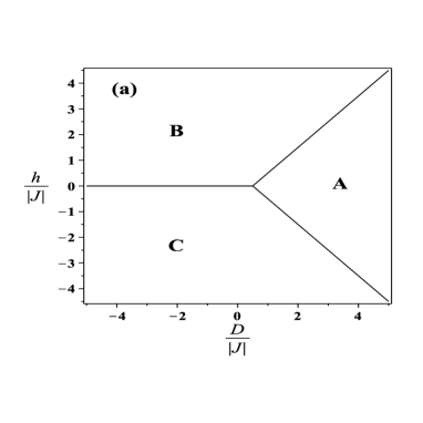
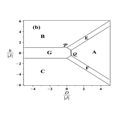
Figure 1: The phase diagrams of the ferromagnetic ($J=-1$) and the anti-ferromagnetic ($J=1$) models (1)/(2) at $T=0$. (a) The ferromagnetic phases represent the following configurations of the $z$-components of the neighbour spins: $\mbox{A}\rightarrow(0,0)$, $\mbox{B}\rightarrow(1,1)$ and $\mbox{C}\rightarrow(-1,-1)$. (b) The AF phases include the configurations A, B and C that are found in the ferromagnetic diagram plus the phases: $\mbox{E}\rightarrow(1,0)$, $\mbox{F}\rightarrow(0,-1)$ and $\mbox{G}\rightarrow(-1,1)$. This diagram has also two tricritical points: ${\mathcal{P}}(\frac{h}{|J|}=1$ and $D=0$) and ${\mathcal{Q}}(\frac{h}{|J|}=\frac{1}{2}$ and $\frac{D}{|J|}=\frac{1}{2}$). The phase diagram of the staggered ferromagnetic and the AF models of the Hamiltonian (4), at $T=0$, are given by the figures ($b$) and ($a$) respectively.

In Fig.1 we present the phase diagram of the ferro ($J=-1$) and AF versions of Hamiltonian (1)/(5) at $T=0$. In its caption we describe the meaning of the phases in each diagram. It is interesting to notice that the exchange coupling term $J$ in the ferromagnetic Hamiltonian (1)/(5) favors the states with $z$ component of the spin $s_{i}^{z}=\mp 1$ and parallel neighboring spins. The same term in the AF version of this Hamiltonian also favors the states with $s_{i}^{z}=\mp 1$ but for anti-parallel (Néel state) neighboring spins. In the ferro and AF models the Zeeman term favors states with $s_{i}^{z}=\mp 1$ aligned with the external magnetic field $h$, whereas the single-ion anisotropy term shows two distinct behaviors: for $D<0$ states with $s_{i}^{z}=\mp 1$ are favored, independently of their relative alignment; and for $D>0$ states with $s_{i}^{z}=0$ are favored, the spin being perpendicular to the external magnetic field applied. For $D<0$ all the terms in Hamiltonian (1)/(5) force the neighboring spins to align to each other and consequently to the external magnetic field at $T=0$. The ground state is a collective stable state under small temperature fluctuations, a point which will be made clear after we discuss the necessary temperature to excite the first excited state of the ferromagnetic chain. For $D>0$ the effect of the crystal field $D$ competes with the exchange strength $J$ and the external magnetic $h$. In the near future we will verify that in this case we need a smaller energy to break the alignment between neighboring spins and excite the first excited energy level of the ferromagnetic chain.

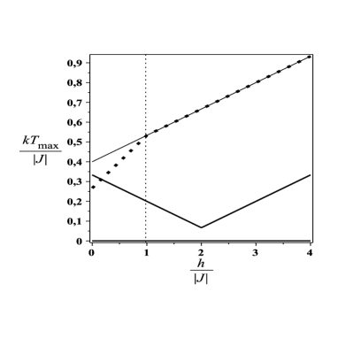
Figure 2: The curves of $\frac{kT_{max}}{|J|}$ for the three distinct first excited states of the ferromagnetic model. The dotted line has $\frac{D}{|J|}=-2$, the solid line has $\frac{D}{|J|}=-\frac{1}{2}$ and the piecewise solid line has $\frac{D}{|J|}=2.5$. The vertical dashed line gives the value of the magnetic field where the first excited state in the ferromagnetic phase A changes.

For $\frac{h}{|J|}\geq 0$ and only for $\frac{D}{|J|}\geq\frac{1}{2}$ the Fig.1a has two distinct phases. The line between the phases is: $\frac{h}{|J|}=\frac{D}{|J|}-\frac{1}{2}$. In the region A of Fig.1a, at $T=0$, the single-ion anisotropy term gives the main contribution to the ground state and the spins are perpendicular to the longitudinal magnetic field. Our phase diagram Fig.1a coincides with Fig.2 of Ref.[12] with $K=0$.

Fig.1b presents the phase diagram of the standard AF model ($J=1$) at $T=0$. For $\frac{D}{|J|}<0$ and $\frac{h}{|J|}\geq 0$ there are two distinct phases that correspond to the competition between the exchange coupling term $J$ and the Zeeman term. One of them is the phase G that is the Néel state when $0\leq\frac{h}{|J|}<1$; the exchange term gives the largest contribution to the ground state energy. For $\frac{D}{|J|}>0$ and $\frac{h}{|J|}\geq 0$ the three terms in the AF Hamiltonian (1)/(5) favor distinct states at $T=0$. Their competition is responsible for a richer phase diagram at $T=0$ for the AF model in this region of parameters. On the other hand, this competition among the terms of Hamiltonian (1)/(5) makes the ground state of the one-dimensional system less stable under small fluctuations of the thermal energy, as we will verify in the discussion of the first excited state of the AF chain. The diagram of this model has two tricritical points: ${\mathcal{P}}(\frac{h}{|J|}=1$ and $D=0$) and ${\mathcal{Q}}(\frac{h}{|J|}=\frac{1}{2}$ and $\frac{D}{|J|}=\frac{1}{2}$) in Fig.1b. For $0<\frac{D}{|J|}<\frac{1}{2}$ and $\frac{h}{|J|}\geq 0$, the AF model has three distinct phases at $T=0$, namely: the G (Néel) phase, the E phase (in which half of the spins in the chain are perpendicular to the external magnetic field), and the B phase (in which all the spins are aligned with the magnetic field). We also have three phases for $\frac{D}{|J|}\geq\frac{1}{2}$, but in this region of the phase diagram at $T=0$ the Néel state is not one of the possible ground states of the system; there is an A phase instead, in which all spins are perpendicular to the longitudinal magnetic field, besides the phases B and E. The phase diagram Fig.1b agrees with Fig.2b of Ref.[8] and shows qualitative agreement with Fig.2 of Ref.[7].

The transitions between the ground states of the standard AF model happen for the following values of magnetic field $\frac{h}{|J|}\geq 0$ and the intervals of $\frac{D}{|J|}$:

$$\mbox{G}\rightleftharpoons\mbox{B}: \frac{D}{|J|}<0 \mbox{and}\hskip 19.91684pt\frac{h}{|J|}=1,$$ (7a)

$$\mbox{G}\rightleftharpoons\mbox{E}: 0<\frac{D}{|J|}<\frac{1}{2} \mbox{and}\hskip 19.91684pt\frac{h}{|J|}=1-\frac{D}{|J|},$$ (7b)

$$\mbox{A}\rightleftharpoons\mbox{E}: \frac{D}{|J|}>\frac{1}{2} \mbox{and}\hskip 19.91684pt\frac{h}{|J|}=\frac{D}{|J|},$$ (7c)

$$\mbox{E}\rightleftharpoons\mbox{B}: \frac{D}{|J|}>0 \mbox{and}\hskip 19.91684pt\frac{h}{|J|}=1+\frac{D}{|J|}.$$ (7d)

The phase diagram of the staggered ferromagnetic ($J=-1$) Hamiltonian (4) at $T=0$ is shown in Fig.1b whereas the diagram of the staggered AF ($J=1$) model at $T=0$ is depicted in Fig.1a.

To the best of our knowledge, there is no detailed discussion in the current literature regarding the presence of plateaus in the $z$-component of the magnetization in $1D$ ferromagnetic spin models at very low temperatures, although its discontinuity is mentioned in Ref.[12]. From the exact expressions of the $z$-component of the magnetizations of the ferro and AF spin-1 classical models, valid in the thermodynamic limit, we verify that they have no discontinuity for $T\stackrel{{\scriptstyle>}}{{{}_{\sim}}}0$. Rather, there is a range of values of the magnetic field for which a continuous transition from one magnetization plateau to another takes place. Our result (6) is equally valid for the ferro and AF models of the standard and staggered spin-1 Ising model with $(S_{i}^{z})^{2}$ term in the presence of a longitudinal magnetic field $T\stackrel{{\scriptstyle>}}{{{}_{\sim}}}0$.

Our result (6) of the HFE of the ferro ($J=-1$) and the AF ($J=1$) Hamiltonians (1)/(5) are valid for $\frac{T}{|J|}>0$. A natural way to describe those models at finite temperature is through their respective density matrix operator. From now on, we restrict our discussions to the condition $\frac{h}{|J|}\geq 0$.

3 The ferromagnetic classical spin-1 model

Let us consider the ferromagnetic model (1)/(5) with $J=-1$. The ground states of the chain at $T=0$ in the phases A, B and C in Fig.1a are

$$|\Psi_{0}\rangle_{A} = |0\rangle_{1}\otimes|0\rangle_{2}\otimes\cdots\otimes|0\rangle_{N},$$ (8a)

$$|\Psi_{0}\rangle_{B} = |1\rangle_{1}\otimes|1\rangle_{2}\otimes\cdots\otimes|1\rangle_{N},$$ (8b)

$$|\Psi_{0}\rangle_{C} = |-1\rangle_{1}\otimes|-1\rangle_{2}\otimes\cdots\otimes|-1\rangle_{N}.$$ (8c)

where $S_{i}^{z}|s\rangle_{i}=s|s\rangle_{i}$, $s=0,\pm 1$ and $i=1,2,\cdots,N$. Their respective ground state energy are named $E_{0}^{A}$, $E_{0}^{B}$ and $E_{0}^{C}$. The ground state (8c) is presented since at $h=0$ its energy degenerates into the energy of the state $|\Psi_{0}\rangle_{A}$.

The values of the ground state energies in units of $|J|$ are

$$\frac{E_{0}^{A}}{|J|} = 0,$$ (9a)

$$\frac{E_{0}^{B}}{|J|} = N\left(-1-\frac{2h}{|J|}+\frac{2D}{|J|}\right),$$ (9b)

$$\frac{E_{0}^{C}}{|J|} = N\left(-1+\frac{2h}{|J|}+\frac{2D}{|J|}\right),$$ (9c)

where $N$ is the number of sites in the chain.

The density matrix operator of the ferromagnetic Hamiltonian (1)/(5) is

$$\rho\left(-1,\frac{D}{|J|},\frac{h}{|J|};\beta\right)=\frac{e^{-\beta E_{0}^{A}}}{Z_{1}}\;|\Psi_{0}\rangle_{A}\phantom{...}{}_{A}\langle\Psi_{0}|+\frac{e^{-\beta E_{0}^{B}}}{Z_{1}}\;|\Psi_{0}\rangle_{B}\phantom{...}{}_{B}\langle\Psi_{0}|+$$

$$\hskip 42.67912pt+\frac{e^{-\beta E_{0}^{C}}}{Z_{1}}\;|\Psi_{0}\rangle_{C}\phantom{...}{}_{C}\langle\Psi_{0}|+\frac{e^{-\beta E_{1}}}{Z_{1}}\times\sum_{l=1}^{N}\;|\Phi_{1}^{(l)}\rangle\langle\Phi_{1}^{(l)}|\cdots,$$ (10)

where $Z_{1}$ is the partition function associated to the ferromagnetic Hamiltonian (1)/(5), $Z_{1}=Tr[e^{-\beta{\mathbf{H}}}]$, with $\beta=\frac{1}{kT}$. $E_{1}$ is the first excited state of the chain and its degeneracy is equal to $N$ for all three ferromagnetic phases. The first excited state is obtained from the ground state vectors (8a)-(8c) by flipping one of its spin-1 in the chain. In the thermodynamic limit, the first excited state is highly degenerate as well the higher excited states[25]. In principle, the contribution of all excited states of the chain should be taken into account for non null temperatures. We have no mathematically sound argument to affirm that, at low temperatures, the expansion (3) should be cut after the contribution of the first excited state. The exact expressions of the thermodynamic functions can be derived from result (6) of the HFE (6) of the HFE, and they show plateaus in the $z$-component of the magnetization of this model at low temperature. The comparison between the exact result and a proposed approximation expression of ${\mathcal{M}}_{z}$ should be able to say how good is the latter.

It is common sense that the the least value of temperature for which the contribution of the first excited state must be taken into account for the behavior of the thermodynamic functions is determined by the factor $e^{-\frac{E_{1}-E_{0}}{kT}}$. But in the present model the excited states have degeneracy at least of order $N$, so all of them should contribute to the functions at non zero temperature.

In the following discussion we determine in each phase of the diagram 1a the value of temperature $T_{max}$ where

$$e^{-\frac{E_{1}-E_{0}}{kT_{max}}}\approx e^{-15}\approx 3.06\times 10^{-7},$$ (11)

where $E_{0}$ is the ground state energy of the phase and $E_{1}$ is its first excited state. Then

$$\frac{kT_{max}}{|J|}\approx\frac{E_{1}-E_{0}}{15}.$$ (12)

We want to verify if the temperature $T_{max}$ at each ferromagnetic phase is such that, for temperatures lower than $T_{max}$, the dependence of the $z$-component of the magnetization on the external magnetic field has a “step-like” form.

We have three distinct first excited states of the ferro classical spin-1 model (1)/(5). They depend on the values of the parameters $\frac{h}{|J|}$ and $\frac{D}{|J|}$.

There are two distinct first excited states in phase B (see Fig.1a):

1.1) for $\frac{h}{|J|}>0$ and $\frac{D}{|J|}\leq-1-\frac{h}{|J|}$

$$|\Phi_{1}^{(l)}\rangle_{B} = |1\rangle_{1}\otimes|1\rangle_{2}\otimes\cdots\otimes|-1\rangle_{l}\otimes\cdots\otimes|1\rangle_{N},\hskip 28.45274ptl=1,2,\cdots,N,$$ (13)

and

$$\frac{E_{1}^{B}-E_{0}^{B}}{|J|}=4\left(1+\frac{h}{|J|}\right).$$ (14)

Replacing the result (14) in eq.(12), we obtain

$$\frac{kT_{max}}{|J|}\approx\frac{4}{15}\left(1+\frac{h}{|J|}\right).$$ (15)

That gives the lowest temperature for which the first excited state is expected to contribute to the behavior of the thermodynamic functions. Eq.(15) shows that $T_{max}$ is independent of the value of $\frac{D}{|J|}$. In this region of parameters of the Hamiltonian (1)/(5), the action of the crystal field $D$ term is more relevant than the exchange coupling term $J$ and the Zeeman term.

1.2) for $\;\;-1-\frac{h}{|J|}\leq\frac{D}{|J|}\leq\frac{1}{2}$ and $\frac{h}{|J|}>0\;\;\cup\;\;\frac{D}{|J|}>\frac{1}{2}$ and $\frac{h}{|J|}\geq\frac{D}{|J|}-\frac{1}{2}$

$$|\Phi_{1}^{(l)}\rangle_{B} = |1\rangle_{1}\otimes|1\rangle_{2}\otimes\cdots\otimes|0\rangle_{l}\otimes\cdots\otimes|1\rangle_{N},\hskip 28.45274ptl=1,2,\cdots,N,$$ (16)

and

$$\frac{E_{1}^{B}-E_{0}^{B}}{|J|}=2\left(1+\frac{h}{|J|}-\frac{D}{|J|}\right).$$ (17)

For this set of parameters $\frac{h}{|J|}$ and $\frac{D}{|J|}$, eq.(12) gives

$$\frac{kT_{max}}{|J|}\approx\frac{2}{15}\left(1+\frac{h}{|J|}-\frac{D}{|J|}\right).$$ (18)

The results (15) and (18) belong to the same phase B and their difference with respect to the first excited state come from the fact that they describe the behavior of the chain of spins-1 in distinct ranges of the parameters of the Hamiltonian: in case (1.1) (case (1.2)) the effect of $\frac{D}{|J|}$ is more (less) important than the exchange coupling and the term Zeeman effect together.

2) the first excited state in phase A (see Fig.1a): $\frac{D}{|J|}\geq\frac{1}{2}$ and $0\leq\frac{h}{|J|}\leq\frac{D}{|J|}-\frac{1}{2}$

$$|\Phi_{1}^{(l)}\rangle_{A} = |0\rangle_{1}\otimes|0\rangle_{2}\otimes\cdots\otimes|1\rangle_{l}\otimes\cdots\otimes|0\rangle_{N},\hskip 28.45274ptl=1,2,\cdots,N,$$ (19)

and

$$\frac{E_{1}^{A}-E_{0}^{A}}{|J|}=2\left(-\frac{h}{|J|}+\frac{D}{|J|}\right).$$ (20)

Replacing the variation of energy (20) in eq.(12), we have

$$\frac{kT_{max}}{|J|}\approx\frac{2}{15}\left(-\frac{h}{|J|}+\frac{D}{|J|}\right).$$ (21)

In the present case the value of $T_{max}$ depends on the value of the crystal field $D$ and $T_{max}$ is a decreasing function of $\frac{h}{|J|}$. The latter implies that the ground state vector (8a) is less stable than the vector (8b) and (8c) under an increasing external magnetic field. In phase A of Fig.1a we have a competition between the crystal field $D$ term and the other two terms in the ferromagnetic Hamiltonian (1)/(5).

In Fig.2 we plot the curves $\frac{kT_{max}}{|J|}$ as a function of $\frac{h}{|J|}$ for three values of $\frac{D}{|J|}$, covering all the regions of $\frac{h}{|J|}\geq 0$ described in the discussion of the first excited states of the ferromagnetic classical spin-1 model (1)/(5). For $\frac{D}{|J|}=2.5$ we have phase A at $T=0$ and there is a competition between the action of the single-ion anisotropy term and the two other terms in the Hamiltonian (1)/(5). For $0\leq\frac{h}{|J|}\leq 2$ we have a negative slope in the curve $\frac{kT_{max}}{|J|}$. This negative slope means that the first excited state can be reached without increasing the temperature.

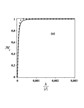
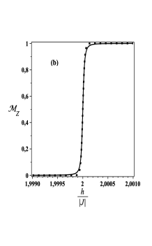
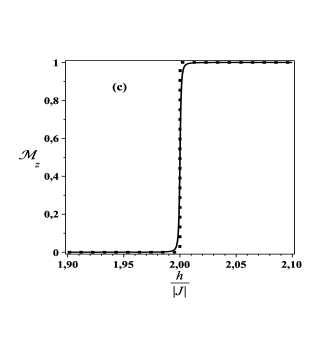
Figure 3: The exact and approximate expressions of ${\mathcal{M}}_{z}$ of the ferromagnetic spin-1 model (1)/(5) versus $\frac{h}{|J|}$. In $(a)$ we have $\frac{D}{|J|}=-2$ at $\frac{kT}{|J|}=0.266$. The solid (dotted) line is its exact (approximate) expression. In $(b)$ we have $\frac{D}{|J|}=2.5$ at $\frac{kT}{|J|}=0.0665$. The solid (dotted) line is its exact (approximate) expression. In $(c)$ we compare the exact expressions of ${\mathcal{M}}_{Z}$ with $\frac{D}{|J|}=2.5$ at temperatures $\frac{kT}{|J|}=0.11$ (solid line) and $0.0665$ (dotted line).

In Figs.3a and 3b we plot the exact curves (solid lines) of ${\mathcal{M}}_{z}\times\frac{h}{|J|}$ with $\frac{D}{|J|}=-2\;\;\mbox{and}\;\;2.5$ at $\frac{kT}{|J|}=0.266\;\;\mbox{and}\;\;0.0665$, respectively. In Fig.3a the $z$-component of the magnetization of the ferromagnetic model begins at null value with $h=0$ and reaches its saturated value ${\mathcal{M}}_{z}=1$ for variations of the magnetic field $\Delta h$ so that $\frac{\Delta h}{|J|}\sim 7\times 10^{-4}$. With $\frac{D}{|J|}=2.5$ the function ${\mathcal{M}}_{z}$ in Fig.3b has a continuous transition from ${\mathcal{M}}_{z}=0$ to ${\mathcal{M}}_{z}=1$ for $\frac{\Delta h}{|J|}\sim 4\times 10^{-4}$. The maximum value of the entropy per site for these two cases is equal to $4.62\times 10^{-3}$ at $h=0$ and $\frac{h}{|J|}=2$. These are the values of the external magnetic field that happens the ferromagnetic phase transitions at $T=0$ in diagram 1a.

In Fig.3c we compare the graphs of the $z$-component of the magnetization of the model with $\frac{D}{|J|}=2.5$ at two different temperatures: $\frac{kT}{|J|}=0.0665$ (dotted line) and $0.11$ (solid line). The latter value of temperature is almost twice the value of $\frac{kT_{max}}{|J|}$ with $h=0$. It is clear from Fig.3b and 3c the presence of the two plateaus at ${\mathcal{M}}_{z}=0$ and ${\mathcal{M}}_{z}=1$ at those low temperatures. These plateaus of ${\mathcal{M}}_{z}$ satisfy the Oshikawa, Yamanaka and Affleck (OYA) condition[26]. We remind that this condition, when applied to the periodic Hamiltonian (1)/(5) with spin-1, imposes that $p(1-{\mathcal{M}}_{z})$ be an integer, where $p$ is the spatial period of the ground state. This is a necessary condition for the occurrence of a plateau in the magnetization curve of the one-dimensional spin system[8, 26]. The same condition is satisfied in Fig.3a. In Fig.3b, the transition between the two plateaus happens at $\frac{h}{|J|}=2$, the value of the magnetic field per unit of $|J|$ in which this ferromagnetic model suffers a transition between the phases A and B at $\frac{D}{|J|}=2.5$. Note that doubling the temperature per unit of $|J|$ does not change much the ”step-like” form of the plateaus in the curve of ${\mathcal{M}}_{z}$. We could say that in the standard ferromagnetic model the plateaus are stiff.

From Figs.3 we verify that outside the transition region $\frac{\Delta h}{|J|}$ where the value of ${\mathcal{M}}_{z}$ suffers a finite transition, the values of this thermodynamic function correspond to their respective value of the ground state in the phase diagram at $T=0$. We can use a phenomenological approach to fit ${\mathcal{M}}_{z}$ in the whole interval of $\frac{h}{|J|}$ at $T\stackrel{{\scriptstyle<}}{{{}_{\sim}}}T_{max}$. We assume that the contributions to ${\mathcal{M}}_{z}$ in the transition region of $\frac{h}{|J|}$ at $T\stackrel{{\scriptstyle<}}{{{}_{\sim}}}T_{max}$ come only from the ground states in the density matrix operator (3). We have two distinct situations to discuss.

Situation 1): $\frac{h}{|J|}\stackrel{{\scriptstyle>}}{{{}_{\sim}}}0$ and $\frac{D}{|J|}\leq\frac{1}{2}$. In this approximation we obtain for $\frac{h}{|J|}\stackrel{{\scriptstyle>}}{{{}_{\sim}}}0$:

$${\mathcal{M}}_{z}(J,D,h;\beta)=\frac{e^{-\beta E_{0}^{B}}-e^{-\beta E_{0}^{C}}}{e^{-\beta E_{0}^{B}}+e^{-\beta E_{0}^{C}}}\;\;\stackrel{{\scriptstyle=}}{{{}_{{}_{E_{0}^{B}<E_{0}^{C}}}}}\;\;\tanh(2\beta Nh).$$ (22)

Since we consider $\frac{h}{|J|}$ to be non-zero and positive we have $E_{0}^{B}<E_{0}^{C}$. We do not have, a priori, a mathematical sound argument to affirm that the approximation (22) gives the right picture of the $z$-component of the magnetization in the ferromagnetic model at low temperatures.

On the last term on the r.h.s. of result (22) we have a product of two limit processes in the region of $\frac{h}{|J|}\sim 0$: $N\rightarrow\infty$ (thermodynamic limit) and $\frac{h}{|J|}\rightarrow 0$. The result (22) depends on the assumption that

$$\lim_{\stackrel{{\scriptstyle N\rightarrow\infty}}{{\frac{h}{|J|}\rightarrow 0}}}N\cdot\frac{h}{|J|}=l(h;\beta),$$ (23)

in which the function $l(h;\beta)$ is assumed to be finite. The simplest phenomenological function $l(h;\beta)$ is a linear function

$$l(h;\beta)=a\cdot\frac{h}{|J|},$$ (24)

where we take $a$ as a constant.

Situation 2: $\frac{h}{|J|}\sim\frac{D}{|J|}-\frac{1}{2}$ and $\frac{D}{|J|}\geq\frac{1}{2}$. Assuming that for $T\stackrel{{\scriptstyle<}}{{{}_{\sim}}}T_{max}$ only the ground states of the ferromagnetic phases A and B contribute to ${\mathcal{M}}_{z}$ , we derive the approximate expression of this thermodynamic function ${\mathcal{M}}_{z}$ valid for $\frac{D}{|J|}\geq\frac{1}{2}$ at low temperature,

$${\mathcal{M}}_{z}(J,D,h;\beta)\approx\frac{e^{-\beta N\varepsilon}}{1+e^{-\beta N\varepsilon}},$$ (25a)

where

$$\varepsilon\equiv 2|J|\left[\frac{h}{|J|}-\left(-\frac{1}{2}+\frac{D}{|J|}\right)\right].$$ (25b)

Again in the exponential functions on the r.h.s. of eq.(25a) we need to calculate the product of two limits in the region $\frac{h}{|J|}\sim\left(-\frac{1}{2}+\frac{D}{|J|}\right)$: $N\rightarrow\infty$ and $\frac{h}{|J|}\rightarrow\left(-\frac{1}{2}+\frac{D}{|J|}\right)$. In analogy to eqs. (23) and (24) we write

$$\lim_{\stackrel{{\scriptstyle N\rightarrow\infty}}{{\frac{h}{|J|}-\left(-\frac{1}{2}+\frac{D}{|J|}\right)\rightarrow 0}}}N\cdot\left[\frac{h}{|J|}-\left(-\frac{1}{2}+\frac{D}{|J|}\right)\right]=l(h;\beta).$$ (26)

In this case we also take the simplest linear function for the phenomenological function $l(h;\beta)$,

$$l(h;\beta)\equiv a\cdot\left[\frac{h}{|J|}-\left(-\frac{1}{2}+\frac{D}{|J|}\right)\right],$$ (27)

where $a$ is a constant.

In Table 1 we present the values of the parameter $a$ for various values of $\frac{D}{|J|}$ at distinct low temperatures. Some of the values of $a$ were used in the approximate curves of ${\mathcal{M}}_{z}$ in Figs.3a and 3b.

4 The antiferromagnetic classical spin-1 model

Fig.1b shows the six distinct phases at T = 0 for the AF spin-1 Ising model with a single-ion anisotropy term in the presence of a longitudinal external magnetic field. With null crystal field ($D=0$), the model has only three different phases at $T=0$.

The three terms in the AF ($J=+1$) Hamiltonian (1)/(5) compete: the exchange coupling term $J$ favors neighbor spins to align anti-parallel. The most stable configurations of the AF ground state happens when the effect of two terms on each spin in the chain are in the same direction.

We present in appendix B the ground state vectors and energies of the six phases of the AF Hamiltonian (1)/(5) at $T=0$ and their respective energy difference between the first excited state and its ground state. We also present in that appendix the relation between $\frac{kT_{max}}{J}$ and the parameters $\frac{h}{J}$ and $\frac{D}{J}$ such that the condition (11) is valid for the classical AF spin-1 model.

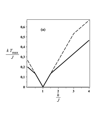
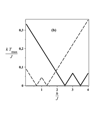
Figure 4: The functions $\frac{kT_{max}}{J}\times\frac{h}{J}$ for the AF classical spin-1 model. In $(a)$ we have the curves with $\frac{D}{J}=-2$ (dashed line) and $\frac{D}{J}=-\frac{1}{2}$ (solid line), and in $(b)$ $\frac{D}{J}=\frac{1}{3}$ (dashed line) and $\frac{D}{J}=2.5$ (solid line)

In Figs.4 we plot the curves of $\frac{kT_{max}}{J}$ for various values of $\frac{D}{J}$ that spans all AF phases at $T=0$ in the phase diagram Fig.1b. The fundamental difference between Figs. 2 and 4 of the ferromagnetic and AF models, respectively, is that the temperature required to excite the first excited ferromagnetic state never vanishes.

In Fig.4a with $\frac{D}{J}<0$ we have $T_{max}=0$ at $\frac{h}{J}=1$. The line $\frac{h}{J}=1$ with $\frac{D}{J}<0$ separates the phases B and G in diagram 1b. The result $T_{max}=0$ along this line means that the classical AF spin-1 model (1)/(5) is gapless along the separation of these two phases.

We also have $T_{max}=0$ in Fig.4b with $\frac{D}{J}=\frac{1}{3}$ at $\frac{h}{J}=\frac{2}{3}$ and $\frac{4}{3}$. These values of $\frac{h}{J}$ are on the lines that separate the phases $E\rightleftharpoons G$ and $B\rightleftharpoons E$ respectively. For the interval $0\leq\frac{D}{J}\leq\frac{1}{2}$ the AF model (1)/(5) is gapless along the lines $\frac{h}{J}=1-\frac{D}{J}$ and $\frac{h}{J}=1+\frac{D}{J}$. At $\frac{h}{J}=2.5$ and $\frac{h}{J}=3.5$ with $\frac{D}{J}=2.5$ we also have $T_{max}=0$ in Fig.4b. These values of $\frac{h}{J}$ are on the lines that separate the phases $A\rightleftharpoons E$ and $B\rightleftharpoons E$ respectively. The AF model (1)/(5) is gapless for $\frac{D}{J}\geq\frac{1}{2}$ along the lines $\frac{h}{J}=\frac{D}{J}$ and $\frac{h}{J}=1+\frac{D}{J}$. We partially summarize the contents of the curves in Figs.4 by saying that the classical AF spin-1 Hamiltonian (1)/(5) is gapless along the lines that separate the phases in the diagram 1b at $T=0$.

The presence of plateaus in the thermodynamic functions ${\mathcal{M}}_{z}$ of the AF Hamiltonian (1) has been reported previously by some authors[7, 8, 10] for positive values of $\frac{D}{J}$[8]. In the following we discuss the behavior of the thermodynamic functions ${\mathcal{M}}_{z}$ and ${\mathcal{S}}$ of the AF version of Hamiltonian (1), that is $J=1$, by varying the value of the crystal field per unit of $J$, $\frac{D}{J}$, to span part of the phase diagram of the AF model (1) at $T=0$ (see Fig.1b).

Here we draw a more detailed comparison between our phase diagram in Fig.1b with the phase diagram of Ref.[8], in which only the case $\frac{D}{J}>0$ is considered. Before we continue the comparison, we should notice that $h_{Chen}=2h$ and $D_{Chen}=2D$, where $h$ and $D$ are our parameters in the Hamiltonian (5). Their Fig.2b agrees with our diagram 1b for $\frac{D}{J}>0$, except for the fact that in their phase diagram the phase ${\mathcal{M}}_{z}=m=0$ does not distinguish the phases A and G (see the caption of our Fig.1b) that correspond to different ground states. In our phase diagram of the AF model we point out the presence of two tricritical points, that is, the points: ${\mathcal{P}}(\frac{h}{J}=1$ and $D=0$) and ${\mathcal{Q}}(\frac{h}{J}=\frac{1}{2}$ and $\frac{D}{J}=\frac{1}{2}$).

For $\frac{D}{J}<0$ and $\frac{h}{|J|}>0$ we have at $T=0$ the phases B and G in diagram 1b for the standard AF model. In this region of parameters of the Hamiltonian we have a competition between the states favored by the exchange coupling term and those favored by the Zeeman term.

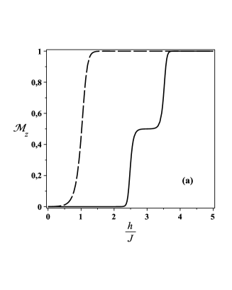
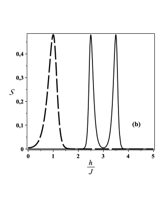
Figure 5: The thermodynamic functions ${\mathcal{M}}_{z}$ and ${\mathcal{S}}$ of the AF spin-1 model (1)/(5) are plotted versus $\frac{h}{J}$ with $\frac{D}{J}=-2$ and $2.5$. $(a)$ ${\mathcal{M}}_{z}$ as a function of $\frac{h}{J}$ with $\frac{D}{J}=-2$ at $\frac{T}{|J|}=0.266$ (long-dashed line) and with $\frac{D}{J}=2.5$ at $\frac{T}{|J|}=0.0665$ (solid line). The entropy per site, ${\mathcal{S}}$, is plotted in ($b$) for the same set of parameters: $\frac{D}{J}=-2$ at $\frac{T}{|J|}=0.266$ (long-dashed line) and $\frac{D}{J}=2.5$ at $\frac{T}{|J|}=0.0665$ (solid line).

Figs.5 show the thermodynamic functions ${\mathcal{M}}_{z}$ and ${\mathcal{S}}$ versus $\frac{h}{J}$ with $\frac{D}{J}=-2$ (long-dashed lines). The $z$-component of the magnetization for $\frac{D}{|J|}<0$ has two plateaus, ${\mathcal{M}}_{z}=0$ and ${\mathcal{M}}_{z}=1$, at very low temperatures. They satisfy the OYA condition[26]. In this region of $\frac{D}{J}$, the transition between these two plateaus happens at $\frac{h}{J}=1$, that is the value in which the transition between the phases B and G at $T=0$ also occurs, for $\frac{D}{J}<0$. Since along any vertical line in this region of $\frac{D}{J}$ only two phases are crossed at $T=0$ (see Fig.1b), the AF spin-1 Ising model (1) has only two plateaus at very low temperatures for $\frac{D}{J}<0$. Fig.5a shows the curve ${\mathcal{M}}_{z}\times\frac{h}{J}$ at $\frac{T}{J}=0.266$, that is the same temperature used in plotting this function for the ferro model in Fig.3a with $\frac{D}{J}=-2$. The curve of ${\mathcal{M}}_{z}$ at $\frac{T}{J}=0.266$ still has little resemblance to a “step-like” function. This behavior differs from that of the magnetization of the standard ferromagnetic model (see Fig.3a). By comparing the behavior of the plateaus in the magnetization in the standard ferro and the AF models at $\frac{T}{J}=0.266$, we can say that the plateaus of the latter smear out even at low temperatures. This happens because although the neighbour spins are aligned (anti-aligned) in phase B (G) the exchange coupling term and the Zeeman term together with the crystal field $D$ compete in promoting opposing effects on these spins. Fig.5b presents the entropy per site with $\frac{D}{J}=-2$ at $\frac{T}{J}=0.266$ (long-dashed line). From this plot we verify that we cannot approximate the function ${\mathcal{M}}_{z}$ by taking into account only the contribution of the two ground states of the phases B and G as was done in the ferromagnetic version of the model. At $\frac{T}{J}=0.266$, the interval $\Delta h$ of the magnetic field for which the transition between the plateaus ${\mathcal{M}}_{z}=0$ and ${\mathcal{M}}_{z}=1$ occurs is such that $\frac{\Delta h}{J}\sim 1$. For temperatures of three orders of magnitude lower, the function ${\mathcal{M}}_{z}$ as a function of $\frac{h}{J}$ has a “step-like” form and $\frac{\Delta h}{J}\sim 10^{-3}$.

Next we consider the AF model (1) with $\frac{D}{|J|}=2.5$. In Fig.5a we plot ${\mathcal{M}}_{z}$ versus $\frac{h}{J}$ at $\frac{T}{J}=0.065$ (solid line). We verify that at this temperature three plateaus still occur; namely, at ${\mathcal{M}}_{z}\in\{0,\frac{1}{2},1\}$, for which the OYA condition is satisfied. We have three plateaus in this case because the vertical line in the diagram 1b, localized at $\frac{D}{|J|}=2.5$, crosses three phases (B, E and G). The values $\frac{h}{J}=2.5$ and $3.5$ where the transitions between the plateaus of the $z$-component of the magnetization occur is the same as that of the transition between the AF phases $\mbox{A}\rightleftharpoons\mbox{E}$ and $\mbox{E}\rightleftharpoons\mbox{B}$, respectively, of the standard model (1) at $T=0$. Also in this case the curve of ${\mathcal{M}}_{z}$ looses its ”step-like” form at $\frac{T}{J}=0.266$. The width of the transition between the plateaus of ${\mathcal{M}}_{z}$ is $\frac{\Delta h}{J}\sim 0.5$ . This width reduces to $10^{-3}$ for temperatures three orders of magnitude lower than $0.0665$

To understand why the AF function ${\mathcal{M}}_{z}$ looses its “step-like” form at $\frac{T}{J}=0.266$ and $0.665$ with $\frac{D}{J}=-2$ and $2.5$ respectively, we plot in Fig.5b the function ${\mathcal{S}}$ as a function of $\frac{h}{J}$ for these two set of parameters. The function ${\mathcal{S}}$ is non-null around $\frac{h}{J}=1$ with $\frac{D}{J}=-2$ (long-dashed line) and around the values $\frac{h}{J}=2.5$ and $3.5$ (solid line). These points in the phase diagram 1b are on the transitions line between the phases $\mbox{A}\rightleftharpoons\mbox{E}$ and $\mbox{E}\rightleftharpoons\mbox{B}$ respectively, of the standard model (1)/(5) with $\frac{D}{J}=2.5$ at $T=0$. Although the AF models are presented at very low temperature, the excited states of the AF model already contribute to the thermodynamic function ${\mathcal{M}}_{z}$ around the values of $\frac{h}{J}$ that correspond to the lines that separate the AF phases in Fig.1b.

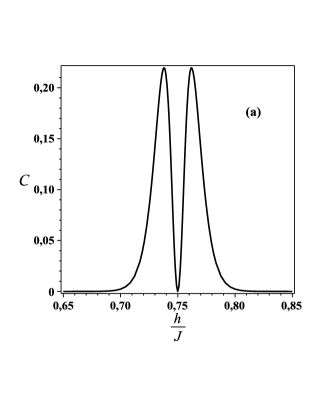
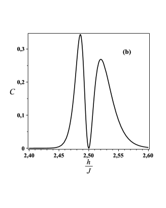
Figure 6: Comparison of the behavior of the function ${\mathcal{C}}\times\frac{h}{J}$ under the transitions $\mbox{G}\rightleftharpoons\mbox{E}$ and $\mbox{A}\rightleftharpoons\mbox{E}$ at low temperature. In $(a)$ we have the transition $\mbox{G}\rightleftharpoons\mbox{E}$ with $\frac{D}{J}=0.25$. In $(b)$ is plotted the specific heat per site of the transition $\mbox{A}\rightleftharpoons\mbox{E}$ with $\frac{D}{J}=2.5$. For both curves we have $\frac{kT}{J}=0.01$.

The curve ${\mathcal{M}}_{z}\times\frac{h}{J}$ with $\frac{D}{J}=\frac{1}{3}$ and $2.5$ are very similar at low temperatures. For $\frac{D}{J}=0.25$, the transition from the plateaus ${\mathcal{M}}_{z}=0$ to ${\mathcal{M}}_{z}=\frac{1}{2}$ corresponds, in the phase diagram 1b, to the transition $\mbox{G}\rightleftharpoons\mbox{E}$, whereas for $\frac{D}{J}=2.5$ (see Fig.5a) the same transition corresponds to the phase crossover $\mbox{A}\rightleftharpoons\mbox{E}$. The magnetization functions are almost insensible if the initial configuration of the spins is either a Néel state or a state with all the spins perpendicular to the longitudinal magnetic field. Comparing Figs.6a and 6b, we see that the specific heat per site, ${\mathcal{C}}(J,h,D;\beta)\left({\mathcal{C}}=-\beta^{2}\;\frac{\partial^{2}[\beta{\mathcal{W}}_{1}]}{\partial\beta^{2}}\right)$ distinguishes the transitions $\mbox{A}\rightleftharpoons\mbox{E}$ and $\mbox{G}\rightleftharpoons\mbox{E}$ at very low temperatures. In Fig.6a the function ${\mathcal{C}}$ is symmetric around $\frac{h}{|J|}=0.75$.

From Fig. 5a we could say that the plateaus of ${\mathcal{M}}_{z}$ in the AF model (1)/(5) are soft, in the sense that they are already smeared out at $\frac{T}{J}=0.26$ and $0.0665$ with $\frac{D}{J}=-2$ and $2.5$ respectively.

Since ${\mathcal{W}}_{1}^{stag}(J,h^{\prime},D^{\prime};\beta)={\mathcal{W}}_{1}(-J,h^{\prime},D^{\prime};\beta)$, we obtain

$${\mathcal{S}}^{stag}(J,h,D;\beta)={\mathcal{S}}(-J,h,D;\beta)$$ (28)

and

$${\mathcal{M}}_{z}^{stag}(J,h,D;\beta)={\mathcal{M}}_{z}(-J,h,D;\beta).$$ (29)

The plateaus in the $z$-component of the magnetization of the standard ferromagnetic (AF) model (1) appear in the $z$-component of the staggered magnetization of the staggered AF (ferromagnetic) model (5). This fact implies that the plateaus in the staggered magnetization of Hamiltonian (4) satisfy the OYA condition, but for this thermodynamic function the AF model has only two plateaus for $\frac{D}{|J|}>0$.

The behavior of the curves of ${\mathcal{S}}^{stag}$ versus $\frac{h}{|J|}$ of the staggered ferro and AF models is identical to the curves of the entropy per site of the standard AF and ferromagnetic models (1)/(5) respectively. It is very simple to understand this situation once the phase diagram at $T=0$ of the staggered ferromagnetic and AF models are depicted by Figs.1b and 1a respectively.

5 Conclusions

The density matrix method[3] and the $\beta$-expansion of the HFE[20] have been applied to the obtainment of the exact expressions of the HFE’s of the one-dimensional standard[21] and the staggered[22] spin-1 Ising models with $(S_{z})^{2}$ term in the presence of a longitudinal magnetic field. The analytic expressions of these functions have been written in terms of exponentials of the parameters of the Hamiltonians (4) and (1)/(5). Our results are valid for their respective ferromagnetic ($J<0$) and AF ($J>0$) models in the interval $T\in(0,\infty)$, extending the results of Ref.[12] to the AF models. These results do not coincide with the results of Ref.[13]. We present the phase diagram of the standard and the staggered spin-models (1)/(5) and (4), respectively, at $T=0$. Our result also gives the exact HFE of the one-dimensional extended Hubbard model in the ionic limit but in the absence of an external magnetic field.

We have studied the behavior of the $z$-component of the magnetization ${\mathcal{M}}_{z}$ and the entropy ${\mathcal{S}}$, both per site, of the ferromagnetic and AF models of Hamiltonian (1)/(5) at low temperatures and their respective staggered versions.

We have presented the two plateaus of ${\mathcal{M}}_{z}$ at low temperatures of the standard ferromagnetic model for $\frac{D}{|J|}>\frac{1}{2}$ and show that the value in which the transition between plateaus at low temperatures occurs is the same as that of diagram 1a.

For the AF model (1)/(2) we show that the number of plateaus of the $z$-component of the magnetization at very low temperatures depends on the number of phases of the model at $T=0$ for a given value of $\frac{D}{|J|}$. Our results for the AF model with $\frac{D}{|J|}>0$ agree with previous results in the literature[7, 10, 8].

The ferromagnetic classical spin-1 model (1)/(5) has has highly degenerate excited states, but we showed that for temperatures $T\stackrel{{\scriptstyle<}}{{{}_{\sim}}}T_{max}$ the function ${\mathcal{M}}_{z}$ can be approximated by the contribution of only two ground states. This fact is not true for the AF model because it is gapless for values of $\frac{h}{J}$ and $\frac{D}{J}$ along the line separating the AF phases in the diagram 1b at $T=0$.

The AF specific heat at very low temperatures distinguishes the phase transitions $\mbox{E}\rightleftharpoons\mbox{G}$ (at $\frac{h}{J}=0.75$) and $\mbox{E}\rightleftharpoons\mbox{B}$ (at $\frac{h}{J}=1.25$) at $\frac{D}{|J|}=0.25$ and $2.5$, respectively, in Figs.6.

By comparing the plots of the ${\mathcal{M}}_{z}$ as a function of $\frac{h}{J}$ at $\frac{T}{|J|}=0.266$ and $0.0665$ to $\frac{D}{J}=-2$ and $2.5$ respectively, we verify that the plateaus of this function of the standard ferro and AF models can be called stiff and soft, respectively.

All the plateaus in the $z$-component of the magnetization of the ferro and AF models of the standard and staggered version satisfy the OYA condition.

As a final comment we should say that the presence of plateaus in the function ${\mathcal{M}}_{z}$ in the classical spin-1 Ising model with single-ion anisotropy term in the presence of a longitudinal magnetic field comes from the stability at low temperature of the ground state vector under the action of increasing the norm of the external magnetic field and the temperature.

S.M.S. (Fellowship CNPq, Brazil, Proc.No.: 303562/2009-9) thanks CNPq and FAPEMIG for the partial financial support. M.T.T. also thanks FAPEMIG. M.T.T. thanks J. Florêncio Jr and J.F. Stilck for enlightening discussions.

Appendix A Calculation of the roots of the third degree
equation of the spin-1 classical model.

Krinsky and Furman applied the transfer matrix method[1, 2, 3] to calculate the HFE of the classical spin-1 model in Ref.[12]. The roots coming from the cubic equations have to be real, but they write them in terms of complex quantities. When we handle those roots numerically these complex quantities may not disappear. In this appendix we recalculate their results for Hamiltonian (1)/(5), showing explicitly that the roots of the cubic equation are real.

Following Ref.[3] we obtain that the partition function ${\mathcal{Z}}_{1}(J,h,D;\beta)$ of the spin-1 Hamiltonian (1)/(5) is equal to

$${\mathcal{Z}}_{1}(J,h,D;\beta)=Tr[{\bf U}^{N}],$$ (A.1)

where $N$ is the number of sites in the periodic chain and the matrix U for the symmetric Hamiltonian (5) is

$${\bf U}(J,h,D;\beta)=\left[\begin{array}[]{c c c}e^{-\beta(J+2h+2D)}&e^{-\beta(h+D)}&e^{-\beta(-J+2D)}\\ e^{-\beta(h+D)}&1&e^{-\beta(-h+D)}\\ e^{-\beta(-J+2D)}&e^{-\beta(-h+D)}&e^{-\beta(J-2h+2D)}\end{array}\right].$$ (A.5)

The matrix ${\bf U}(J,h,D;\beta)$ is hermitian for any value of $J$, $h$, $D$ and $\beta$. Its three eigenvalues $\lambda_{i}$, $i=1,2$ and $3$, are real. The matrices ${\bf U}$ (see eq.(A.5)) and ${\bf T}$ (in Ref.[12]) differ by a rearrangement of lines, only.

In terms of the eigenvalues of U, the partition function (A.1) becomes:

$${\mathcal{Z}}_{1}(J,h,D;\beta)=(\lambda_{1})^{N}\left[1+\left(\frac{\lambda_{2}}{\lambda_{1}}\right)^{N}+\left(\frac{\lambda_{3}}{\lambda_{1}}\right)^{N}\right],$$ (A.6)

in which $\lambda_{1}$ is assumed to be the eigenvalue of matrix U with the largest modulus.

In the thermodynamic limit ($N\rightarrow\infty$), the partition function (A.1) of the model is

$${\mathcal{Z}}_{1}(J,h,D;\beta)=(\lambda_{1})^{N},$$ (A.7)

for non-degenerate eigenvalues of U. The HFE of the model is

$${\mathcal{W}}_{1}(J,h,D;\beta)=-\frac{1}{\beta}\;\;\ln[\lambda_{1}(J,h,D;\beta)].$$ (A.8)

The eigenvalues $\lambda_{i}$, $i=1,2,3$, are roots of the cubic equation

$$-\lambda^{3}+P\lambda^{2}+Q\lambda+R=0,$$ (A.9)

where

$$P = 1+2e^{-\beta(J+2D)}\cosh(2\beta h)=tr[{\bf U}]$$ (A.10a)

$$Q = 4e^{-2\beta D}\;\;e^{-\frac{\beta J}{2}}\cosh(2\beta h)\sinh\left(\frac{\beta J}{2}\right)+2e^{-4\beta D}\;\;\sinh(2\beta J),$$ (A.10b)

$$R = -8e^{-4\beta D}\left[\sinh\left(\frac{\beta J}{2}\right)\right]^{2}\;\;\sinh(\beta J).$$ (A.10c)

The roots of the cubic equation (A.9) are well known[23]

$$s_{1} = 2\sqrt{-\tilde{Q}}\;\;\cos\left(\frac{\theta}{3}\right)+\frac{P}{3},$$ (A.11a)

$$s_{2} = 2\sqrt{-\tilde{Q}}\;\;\cos\left(\frac{\theta}{3}+\frac{2\pi}{3}\right)+\frac{P}{3},$$ (A.11b)

$$s_{3} = 2\sqrt{-\tilde{Q}}\;\;\cos\left(\frac{\theta}{3}-\frac{2\pi}{3}\right)+\frac{P}{3},$$ (A.11c)

where

$$\cos(\theta)=\frac{\tilde{R}}{\sqrt{(-\tilde{Q})^{3}}}$$ (A.12a)

with

$$\tilde{Q}=-\frac{3Q+P^{2}}{9}$$ (A.12b)

and

$$\tilde{R}=\frac{9QP+27R+2P^{3}}{54}.$$ (A.12c)

Our previous result $s_{1}$ does not agree with the expression of $\lambda_{max}$ of Ref.[13]; we believe that there are some misprints in their eqs.(18)-(24).

Appendix B The ground states of the classical AF spin-1 and the calculation of $T_{max}$

For the AF version of the Hamiltonian (1)/(5) we assume that the chain has a even number of sites. Let $N=2M$, in which $M$ is a positive integer. In the thermodynamic limit ($N\rightarrow\infty$) we have $M\rightarrow\infty$.

The ground state vectors at each phase in the diagram 1b at $T=0$ are

$$|\Psi_{0}\rangle_{A} = |0\rangle_{1}\otimes|0\rangle_{2}\otimes\cdots\otimes|0\rangle_{2M},$$ (B.1a)

$$|\Psi_{0}\rangle_{B} = |1\rangle_{1}\otimes|1\rangle_{2}\otimes\cdots\otimes|1\rangle_{2M},$$ (B.1b)

$$|\Psi_{0}\rangle_{C} = |-1\rangle_{1}\otimes|-1\rangle_{2}\otimes\cdots\otimes|-1\rangle_{V},$$ (B.1c)

$$|\Psi_{0}\rangle_{E} = |0\rangle_{1}\otimes|1\rangle_{2}\otimes|0\rangle_{3}\otimes|1\rangle_{4}\otimes\cdots\otimes|0\rangle_{2M-1}|1\rangle_{2M},$$ (B.1d)

$$|\Psi_{0}\rangle_{F} = |0\rangle_{1}\otimes|-1\rangle_{2}\otimes|0\rangle_{3}\otimes|-1\rangle_{4}\otimes\cdots\otimes|0\rangle_{2M-1}|-1\rangle_{2M},$$ (B.1e)

$$|\Psi_{0}\rangle_{G} = |1\rangle_{1}\otimes|-1\rangle_{2}\otimes|1\rangle_{3}\otimes|-1\rangle_{4}\otimes\cdots\otimes|1\rangle_{2M-1}|-1\rangle_{2M}.$$ (B.1f)

One is reminded that $S_{i}^{z}|s\rangle_{i}=s|s\rangle_{i}$, $s=0,\pm 1$ and $i=1,2,\cdots 2M$.

We are interested in the discussion of the thermodynamic function ${\mathcal{M}}_{z}$ at low temperatures. This function has an even dependence on $\frac{h}{J}$; then we restrict our discussion to $\frac{h}{J}\geq 0$. In the following we do not mention the quantum behavior of the phases C and F at low temperature.

The value of the ground state energy of the phases A, B, E and G are, respectively,

$$\frac{E_{0}^{A}}{J} = 0,$$ (B.2a)

$$\frac{E_{0}^{B}}{J} = N\left(1+\frac{2D}{J}-\frac{2h}{J}\right),$$ (B.2b)

$$\frac{E_{0}^{E}}{J} = N\left(\frac{D}{J}-\frac{h}{J}\right),$$ (B.2c)

$$\frac{E_{0}^{G}}{J} = N\left(-1+\frac{2D}{J}\right).$$ (B.2d)

We have a much more complex distribution of first excited states $E_{1}$ in the AF spin-1 Ising model (1)/(5) than in the ferromagnetic version of the model.

Let us present the difference between the first excited and the ground states of each phase A, B, E and G in diagram 1b.

1) Phase A: $\frac{D}{J}\geq\frac{1}{2}$ and $\frac{h}{J}\leq\frac{D}{J}$. We have

$$\frac{E_{1}-E_{0}^{A}}{J}=2\left(-\frac{h}{J}+\frac{D}{J}\right),$$ (B.3)

which is substituted in eq.(12) to give

$$\frac{kT_{max}}{J}\approx\frac{2}{15}\left(-\frac{h}{J}+\frac{D}{J}\right).$$ (B.4)

2) Phase B: we have two distinct first excited states

2.1) $\frac{D}{J}\leq 0$ and $\frac{h}{J}\geq 1-\frac{D}{J}\;\;\cup\;\;\frac{D}{J}\geq 0$ and $\frac{h}{J}\geq 1+\frac{D}{J}$. Then

$$\frac{E_{1}-E_{0}^{B}}{J}=2\left(-1+\frac{h}{J}-\frac{D}{J}\right)$$ (B.5)

and eq.(12) gives

$$\frac{kT_{max}}{J}\approx\frac{2}{15}\left(-1+\frac{h}{J}-\frac{D}{J}\right).$$ (B.6)

2.2) $\frac{D}{J}\leq 0$ and $1\leq\frac{h}{J}\leq 1-\frac{D}{J}$. Then

$$\frac{E_{1}-E_{0}^{B}}{J}=4\left(-1+\frac{h}{J}\right),$$ (B.7)

and eq.(12) becomes

$$\frac{kT_{max}}{J}\approx\frac{4}{15}\left(-1+\frac{h}{J}\right).$$ (B.8)

3) Phase E: in this phase we have three distinct first excited states.

3.1) $0\leq\frac{D}{J}\leq\frac{1}{2}$ and $1-\frac{D}{J}\leq\frac{h}{J}\leq 1$. We have

$$\frac{E_{1}-E_{0}^{E}}{J}=2\left(-1+\frac{h}{J}+\frac{D}{J}\right),$$ (B.9)

with eq.(12) giving

$$\frac{kT_{max}}{J}\approx\frac{2}{15}\left(-1+\frac{h}{J}+\frac{D}{J}\right),$$ (B.10)

3.2) $0\leq\frac{D}{J}\leq\frac{1}{2}$ and $1\leq\frac{h}{J}\leq 1+\frac{D}{J}\;\;\cup\;\;\frac{D}{J}\geq\frac{1}{2}$ and $\frac{1}{2}+\frac{D}{J}\leq\frac{h}{J}\leq 1+\frac{D}{J}$. We have

$$\frac{E_{1}-E_{0}^{E}}{J}=2\left(1-\frac{h}{J}+\frac{D}{J}\right),$$ (B.11)

which gives

$$\frac{kT_{max}}{J}\approx\frac{2}{15}\left(1-\frac{h}{J}+\frac{D}{J}\right).$$ (B.12)

3.3) $\frac{1}{2}\leq\frac{D}{J}\leq 1$ and $1\leq\frac{h}{J}\leq\frac{1}{2}+\frac{D}{J}\;\;\cup\;\;\frac{D}{J}\geq 1$ and $\frac{D}{J}\leq\frac{h}{J}\leq\frac{1}{2}+\frac{D}{J}$. We have

$$\frac{E_{1}-E_{0}^{E}}{J}=2\left(\frac{h}{J}-\frac{D}{J}\right),$$ (B.13)

that substituted in eq.(12) gives

$$\frac{kT_{max}}{J}\approx\frac{2}{15}\left(\frac{h}{J}-\frac{D}{J}\right).$$ (B.14)

4) Phase G: in this phase we have two distinct first excited states.

4.1) $\frac{D}{J}\leq-1$ and $0\leq\frac{h}{J}\leq 1\;\;\cup\;\;-1\leq\frac{D}{J}\leq 0$ and $\frac{h}{J}\leq 1+\frac{D}{J}$. We have

$$\frac{E_{1}-E_{0}^{G}}{J}=4\left(1-\frac{h}{J}\right).$$ (B.15)

From eq.(12) we obtain

$$\frac{kT_{max}}{J}\approx\frac{4}{15}\left(1-\frac{h}{J}\right).$$ (B.16)

4.2) $-1\leq\frac{D}{J}\leq 0$ and $\frac{h}{J}\leq 1+\frac{D}{J}\;\;\cup\;\;0\leq\frac{D}{J}\leq\frac{1}{2}$ and $\frac{1}{2}\leq\frac{h}{J}\leq 1-\frac{D}{J}\;\;\cup\;\;0\leq\frac{D}{J}\leq\frac{1}{2}$ and $0\leq\frac{h}{J}\leq\frac{1}{2}$. We have

$$\frac{E_{1}-E_{0}^{G}}{J}=2\left(1-\frac{h}{J}-\frac{D}{J}\right),$$ (B.17)

with eq.(12) given

$$\frac{kT_{max}}{J}\approx\frac{2}{15}\left(1-\frac{h}{J}-\frac{D}{J}\right).$$ (B.18)

$\frac{D}{|J|}$	$\frac{kT}{|J|}$	A	$\frac{\Delta h}{|J|}$
-2	0.06	$2.9\cdot 10^{14}$	$1.3\cdot 10^{-15}$
	0.133	$3.39\cdot 10^{6}$	$1.8\cdot 10^{-7}$
	0.266	$1.842\cdot 10^{3}$	$6.7\cdot 10^{-4}$
$-\frac{1}{2}$	0.0665	$1.15\cdot 10^{13}$	$2.9\cdot 10^{-14}$
	0.1995	$2.25\cdot 10^{4}$	$4\cdot 10^{-6}$
2.5	0.04	$4.9\cdot 10^{5}$	$10^{-6}$
	0.0665	$3.42\cdot 10^{3}$	$10^{-3}$

Table 1: The values of the parameter $a$ in eqs.(24) and (27) for several values of $\frac{D}{|J|}$ and different values of temperature. $\frac{\Delta h}{|J|}$ is the interval of variation of the magnetic field in which the function ${\mathcal{M}}_{z}$ varies continuously between ${\mathcal{M}}_{z}=0$ and ${\mathcal{M}}_{z}=1$.

References

- [1] H.A. Kramers and G.H. Wannier, Phys. Rev. 60 (1941) 252.
- [2] H.A. Kramers and G.H. Wannier, Phys. Rev. 60 (1941) 263.
- [3] R.J. Baxter, ”Exactly Solved Models in Statistical Mechanics”, Academic Press (1989), section 2.1.
- [4] J. Simon et al., Nature 472, 04/21/2011, p. 307, and references therein.
- [5] M. Blume, Phys. Rev. 141 (1966) 517.
- [6] H.W. Capel, Physica (Utrecht) 32 (1966) 966; 33 (1967) 295.
- [7] E. Aydiner and C. Akyüz, Chin. Phys. Lett. 22 (2005) 2382.
- [8] X.Y. Chen et al, J. of Mag. and Mag. Mat 262 (2003) 258.
- [9] F. Mancini, Europhys. Lett. 70 (2005) 485.
- [10] F. Mancini and F.P. Mancini, Cond. Matt. Phys. 11 (2008) 543.
- [11] W.A. Moura-Melo et al., Phys. A 322 (2003) 393. Please notice a misprint in eq.(28) of this reference: the correct coefficient of the term , inside the square root, is .
- [12] S. Krinsky and D. Furman, Phys. Rev. B11 (1975) 2602.
- [13] F. Litaiff, R. de Sousa and N.S. Branco, Solid State Communication 147 (2008) 494.
- [14] C.Ekiz, H. Yaraneri, J. of Mag. and Mag. Mat 318 (2007) 49, and references therein.
- [15] Y. Narumi et al., Phys. B246 (1998) 509.
- [16] Y. Narume et al., J. of Mag. and Mag. Mat 177-181 (1998) 685.
- [17] T. Goto et al.. Phys. B294-295 (2001) 43.
- [18] D. Luz, R.R. dos Santos, Phys. Rev. B54 (1996) 1302.
- [19] M. Moutinho, E.V. Corr a Silva and M.T. Thomaz, Phys. A336 (2004) 477.
- [20] O. Rojas, S. M. de Souza, and M. T. Thomaz, J. Math. Phys. 43 (2002) 1390.
-
[21]
M.T. Thomaz and O. Rojas, Condensed Matter
Physics 15 (2012) 13706: 110
[dx.doi.org/10.5488/CMP.15.13706, http://www.icmp.lviv.ua/journal]. - [22] E.V. Corrêa Silva, S.M de Souza and M.T. Thomaz, Phys. A390 (2011) 3108.
- [23] M.R. Spiegel, ”Mathematical Handbook of Formula and Tables”, Schaum’s Outline Series, Singapore (1990), page 32.
- [24] The factor in the relation between and comes from the symmetric form of Hamiltonian (5) in the sites and .
- [25] F.C. Alcaraz, S.R. Salinas and W.F. Wreszinski, Phys. Rev. Lett. 75 (1995) 930.
- [26] M. Oshikawa, M. Yamanaka and I. Affleck, Phys. Rev. Lett. 78 (1997) 1984.