Evolution of CO lines in time-dependent models of protostellar disk formation

Context. Star and planet formation theories predict an evolution in the density, temperature, and velocity structure as the envelope collapses and forms an accretion disk. While continuum emission can trace the dust evolution, spectrally resolved molecular lines are needed to determine the physical structure and collapse dynamics.
Aims. The aim of this work is to model the evolution of the molecular excitation, line profiles, and related observables during low-mass star formation. Specifically, the signatures of disks during the deeply embedded stage ($M_{\rm env}>M_{\star}$) are investigated.
Methods. The semi-analytic 2D axisymmetric model of Visser and collaborators has been used to describe the evolution of the density, stellar mass, and luminosity from the pre-stellar to the T-Tauri phase. A full radiative transfer calculation is carried out to accurately determine the time-dependent dust temperatures. The time-dependent CO abundance is obtained from the adsorption and thermal desorption chemistry. Non-LTE near-IR, FIR, and submm lines of CO have been simulated at a number of time steps.
Results. In single dish (10–20^′′ beams), the dynamics during the collapse are best probed through highly excited ¹³CO  and C¹⁸O lines, which are significantly broadened by the infall process. In contrast to the dust temperature, the CO excitation temperature derived from submm/FIR data does not vary during the protostellar evolution, consistent with C¹⁸O observations obtained with Herschel and from ground-based telescopes. The near-IR spectra provide complementary information to the submm lines by probing not only the cold outer envelope but also the warm inner region. The near-IR high-$J$ ($\geq 8$) absorption lines are particularly sensitive to the physical structure of the inner few AU, which does show evolution. The models indicate that observations of ¹³CO and C¹⁸O low-$J$ submm lines within a $\leq$1$\arcsec$ (at 140 pc) beam are well suited to probe embedded disks in Stage I ($M_{\rm env}<M_{\star}$) sources, consistent with recent interferometric observations. High signal-to-noise ratio subarcsec resolution data with ALMA are needed to detect the presence of small rotationally supported disks during the Stage 0 phase and various diagnostics are discussed. The combination of spatially and spectrally resolved lines with ALMA and at near-IR is a powerful method to probe the inner envelope and disk formation process during the embedded phase.

1 Introduction

The semi-analytical model of the collapse of protostellar envelopes (Shu 1977; Cassen & Moosman 1981; Terebey et al. 1984) has been used extensively to study the evolution of gas and dust from core to disk and star (Young & Evans 2005; Dunham et al. 2010; Visser et al. 2009). Others have explored the effects of envelope and disk parameters representative of specific evolutionary stages on the spectral energy distribution (SED) and other diagnostics (Whitney et al. 2003; Robitaille et al. 2006, 2007; Crapsi et al. 2008; Tobin et al. 2011). These studies have focused primarily on the dust emission and its relation to the physical structure. On the other hand, spectroscopic observations toward young stellar objects (YSOs) performed by many ground-based (sub)millimeter and infrared telescopes also contain information on the gas structure (Evans 1999). The molecular lines are important in revealing the kinematical information of the collapsing envelope as well as the physical parameters of the gas based on the molecular excitation. The Herschel Space Observatory and the Atacama Large Millimeter/submillimeter Array (ALMA) provide new probes of the excitation and kinematics of the gas on smaller scales and up to higher temperatures than previously possible. It is therefore timely to simulate the predicted molecular excitation and line profiles within the standard picture of a collapsing envelope. The aim is to identify diagnostic signatures of the different physical components and stages and to provide a reference for studies of more complex collapse dynamics.

A problem that is very closely connected to the collapse of protostellar envelopes is the formation of accretion disks. The presence of embedded disks was inferred from the excess of continuum emission at the smallest spatial scales through interferometric observations (eg. Keene & Masson 1990; Brown et al. 2000; Jørgensen et al. 2005, 2009). Their physical structure can be determined by the combined modeling of the SED and the interferometric observations (Jørgensen et al. 2005; Brinch et al. 2007; Enoch et al. 2009). However, the excess continuum emission at small scales can also be due to other effects of a (magnetized) collapsing rotating envelope (pseudo-disk, Chiang et al. 2008). Therefore, resolved molecular line observations from interferometers such as ALMA are needed to clearly detect the presence or absence of a stable rotating embedded disk (Brinch et al. 2007, 2008; Lommen et al. 2008; Jørgensen et al. 2009; Tobin et al. 2012).

A number of previous studies have modeled the line profiles based on the spherically symmetry inside-out collapse scenario described by Shu (1977) (eg., Zhou et al. 1993; Hogerheijde & Sandell 2000; Hogerheijde 2001; Lee et al. 2004, 2005; Evans et al. 2005). Also, numerical hydrodynamical collapse models have been coupled with chemistry and line radiative transfer to study the molecular line evolution in 1D (Aikawa et al. 2008) and 2D (Brinch et al. 2007; van Weeren et al. 2009). Best-fit collapse parameters (e.g., sound speed and age) are obtained but depend on the temperature structure and abundance profile of the model. Visser et al. (2009) and Visser & Dullemond (2010) developed 2D semi-analytical models that describe the density and velocity structure as matter moves onto and through the forming disk. This model has been coupled with chemistry (Visser et al. 2009, 2011), but no line profiles have yet been simulated. The current paper presents the first study of the CO molecular line evolution within 2D disk formation models. CO and its isotopologs are chosen because it is a chemically stable molecule and readily observed.

Observationally, most early studies of low-mass embedded YSOs focused on the low$-J$ ($J_{\rm u}\leq 6$) (sub-)millimeter CO lines in 20–30$\arcsec$ beams, thus probing scales of a few thousand AU in the nearest star-forming regions (e.g., Belloche et al. 2002; Jørgensen et al. 2002; Lee et al. 2004; Young et al. 2004; Crapsi et al. 2005). More recently, ground-based high-frequency observations of large samples up to $J_{\rm u}$=7 are becoming routinely available (Hogerheijde et al. 1998; van Kempen et al. 2009a, b, c) and Herschel-HIFI (de Graauw et al. 2010) has opened up spectrally resolved observations of CO and its isotopologs up to $J_{\rm u}=16$ ($E_{\rm u}=660$ K) (Yıldız et al. 2010, 2012). In addition, the PACS (Poglitsch et al. 2010) and SPIRE (Griffin et al. 2010) instruments provide spectrally unresolved CO data from $J_{\rm u}=4$ to $J_{\rm u}=50$ ($E_{\rm u}=55-7300$ K), revealing multiple temperature components (e.g., van Kempen et al. 2010; Herczeg et al. 2012; Goicoechea et al. 2012; Manoj et al. 2013). Although the interpretation of the higher lines requires additional physical processes than those considered here (Visser et al. 2012), our models provide a reference frame within which to analyze the lower-$J$ lines.

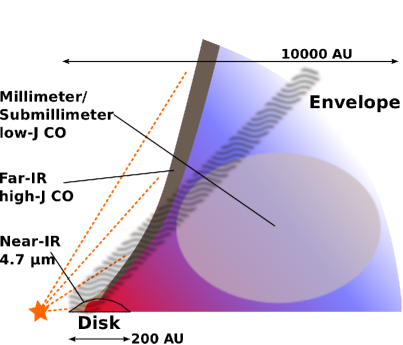
Figure 1: Sketch of one quadrant of an embedded protostellar system with a disk and envelope. The FIR/millimeter/submillimeter emission comes from the envelope and outflow cavity walls. On the other hand, the NIR absorption (gray shaded region) also probes the warm region close to the star through a pencil beam, illustrating the complementarity of the techniques. The dotted orange lines indicate the stellar light.

Complementary information on the CO excitation is obtained from near-IR (NIR) observations of the 4.7 $\mu$m fundamental CO (v=1–0) band seen in absorption toward YSOs. Because the absorption probes a pencil beam line of sight toward the central source, the lines are more sensitive to the inner dense part of the envelope than the submillimeter emission line data, which are dominated by the outer envelope (see Fig. 1). The NIR data generally reveal a cold ($<30$ K) and a warm ($>90$ K) component (Mitchell et al. 1990; Boogert et al. 2002; Brittain et al. 2005; Smith et al. 2009; Herczeg et al. 2011). The cold component is seen toward all YSOs in all of the isotopolog absorptions. However, the warm temperature varies from source to source. The question is whether the standard picture of collapse and disk formation can also reproduce these multiple temperature components.

A description of the physical models and methods is given in Section 2. The evolution of the molecular excitation and the resulting far-infrared (FIR) to submm lines of the pure rotational transitions of CO is discussed in Section 3, whereas the NIR ro-vibrational transitions is presented in Section 4. The implication of the results and whether embedded disks can be observed during Stage 0 is discussed in Section 5. The results and conclusions are summarized in Section 6.

2 Method

2.1 Physical structure

Table 1: Parameters used for the three different evolutionary models.

Model	$\Omega_{0}$	$c_{\mathrm{s}}$	$r_{\mathrm{env}}$	$t_{\mathrm{acc}}$	$M_{\mathrm{d}}$	$R_{\mathrm{d},\mathrm{out}}$
	[Hz]	[km s-1]	[AU]	[$10^{5}$ yr]	[$M_{\odot}$]	[AU]
1	$10^{-14}$	0.26	6700	2.5	0.1	50
2	$10^{-14}$	0.19	12000	6.3	0.2	180
3	$10^{-13}$	0.26	6700	2.5	0.4	325

The two-dimensional axisymmetric model of Visser et al. (2009), Visser & Dullemond (2010) and Visser et al. (2011) was used to simulate the collapse of a rotating isothermal spherical envelope into a pre-main sequence star with a circumstellar disk. The model is based on the analytical collapse solutions of Shu (1977, hereafter S77), Cassen & Moosman (1981, hereafter CM81) and Terebey et al. (1984, hereafter TSC84). The formation and evolution of the disk follow according to the $\alpha_{S}$ viscosity prescription, which includes conservation of angular momentum (Shakura & Sunyaev 1973; Lynden-Bell & Pringle 1974). The dust temperature structure ($T_{\mathrm{dust}}$) is a key quantity for the chemical evolution, so it is calculated through full 3D continuum radiative transfer with RADMC3D, considering the protostellar luminosity as the only heating source. The gas temperature is set equal to the dust temperature, which has been found to be a good assumption for submm molecular lines (Doty et al. 2002, 2004).

The model is modified slightly in order to be consistent with observational constraints. The density at $r=1000$ AU ($n_{1000}$) should be at most $10^{6}$ cm^-3 for envelopes around low-mass YSOs (Jørgensen et al. 2002; Kristensen et al. 2012), but the interpolation scheme of Visser et al. (2009) violated that criterion. To correct this, the CM81 and TSC84 solutions are connected in terms of the dimension-less variable $\tau=\Omega_{0}t$ by interpolating between $100\tau^{2}$ and $10\tau^{2}$ for $\Omega_{0}=10^{-13}$ Hz and between 100$\tau^{2}$ and $\tau^{2}$ for $\Omega_{0}=10^{-14}$ Hz, where $\Omega_{0}$ is the envelope’s initial solid body rotation rate. The overall collapse, the structure of the disk and the chemical evolution are unaffected by this modification. The models evolve until one accretion time, $t_{\rm acc}=M_{0}/\dot{M}$ where $\dot{M}\propto c_{\rm s}^{3}/G$ with $c_{\rm s}$ the initial effective sound speed of the envelope, which is tabulated in Table 1.

Three different sets of initial conditions are used in this work (Table 1), which are a subset of the conditions explored by Visser et al. (2009) and Visser & Dullemond (2010). Each model begins with a 1 $M_{\odot}$ envelope. The two variables $\Omega_{0}$ and $c_{\mathrm{s}}$ affect the final disk structure and mass. Model 1 ($c_{\mathrm{s}}=0.26$ km s^-1, $\Omega_{0}=10^{-14}$ Hz) produces a disk with a final mass ($t/t_{\rm acc}=1$) of 0.1 $M_{\odot}$ and a final radius of 50 AU. Changing $\Omega_{0}$ to $10^{-13}$ Hz (Model 3) yields the most massive and largest of the three disks (0.4 $M_{\odot}$, 325 AU). Starting with a lower sound speed of 0.19 km s^-1 (Model 2) produces a disk of intermediate mass and size (0.2 $M_{\odot}$, 180 AU). The initial conditions also affect the flattened inner envelope structure. In Model 3, the flattening of the inner envelope extends to $>300$ AU by $t/t_{\mathrm{acc}}=0.5$ and extends up to $\sim$1000 AU by the end of the accretion phase. In the other two models, the extent of the flattening is similar to the extent of the disk, with Model 2 showing more flattening in the inner envelope than Model 1. The different evolutionary stages are characterized by the relative masses in the different components (Robitaille et al. 2006): $M_{\rm env}>>M_{\star}$ (Stage 0, $t/t_{\rm acc}\leq 0.5$), $M_{\rm env}<M_{\star}$ but $M_{\rm env}>M_{\rm disk}$ (Stage 1, $t/t_{\rm acc}>0.5$) and $M_{\rm env}<M_{\rm disk}$ (Stage 2) (see Appendix B).

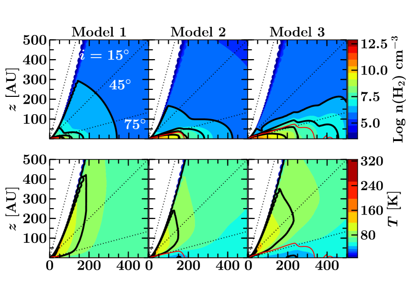
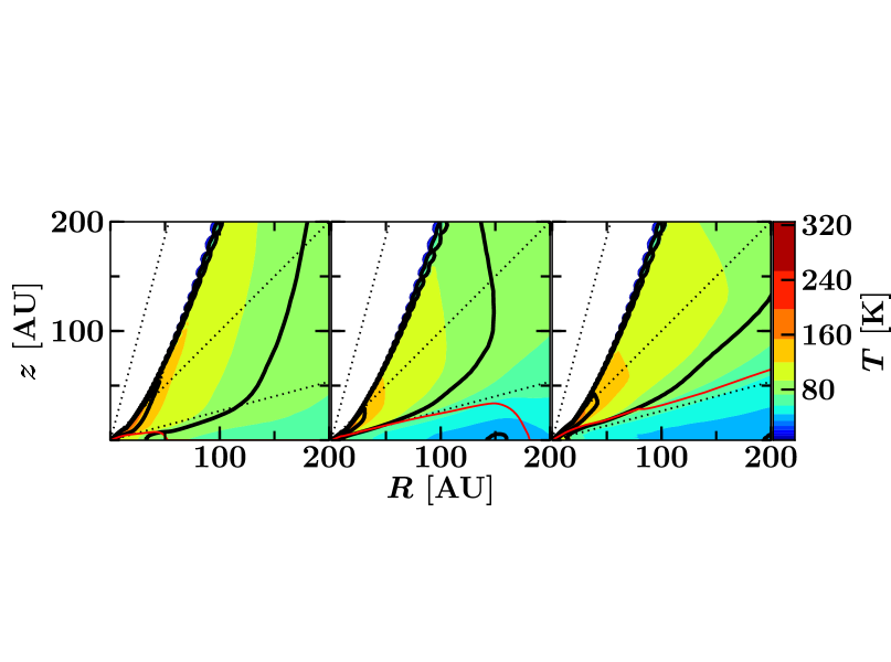
Figure 2: Final disk structure for the three models from Table 1 at $t=t_{\mathrm{acc}}$. Top: gas density in the inner 500 AU. The solid line contours mark densities of $10^{6,7,8,9}$ cm^-3. Middle: temperature structure in the inner 500 AU. The temperature contours are logarithmically spaced from 10 to 320 K. The 20, 50 and 100 K isotherms are marked by the solid line contours. Bottom: temperature structure in the inner 200 AU. In all panels, the dotted lines illustrate the lines of sight at inclinations of 15^∘, 45^∘ and 75^∘ and the red line indicates the final disk surface.

Our main purpose is to investigate how the molecular lines evolve during different disk formation scenarios (Stage 0/I). Hence, the parameters were chosen to explore the formation of three different disk structures. Figure 2 zooms in on the final disk structures for the different models at the accretion time ($t=t_{\mathrm{acc}}$) where the red lines outline the disk surfaces. The angular velocities within these lines are assumed to be Keplerian while regions outside these lines are described by the analytical collapsing rotating envelope solutions (Visser et al. 2009). The density structure is 2D axisymmetric with a 3D velocity field within the envelope and the disk.

2.2 CO abundance

The ¹²CO abundance is obtained through the adsorption and thermal desorption chemistry as described in Section  2.7 of Visser et al. (2009). The main difference is that we have used both the forward and backward methods (Visser et al. 2011) to sample the trajectories through the disk and envelope. The chemistry is still solved in the forward direction.

CO completely freezes out at $T_{\mathrm{d}}\leq 18$ K (Visser et al. 2009). For the majority of the time steps used for the molecular line simulations, the dust temperature is well above 18 K everywhere except for the outer envelope beyond $\sim$4000 AU. However, due to the low densities within this region, CO is still predominantly in the gas phase. Only at early time steps, early Stage 0, a large fraction of CO is frozen out within the inner envelope. Constant isotope ratios of ${}^{12}{\rm C}/^{13}{\rm C}=70$ and ${}^{16}{\rm O}/^{18}{\rm O}=540$ (Wilson & Rood 1994) are used throughout the model to compute the abundances of ¹³CO and C¹⁸O.

2.3 Line radiative transfer

A fast and accurate multi-dimensional molecular excitation and radiative transfer code is needed to obtain observables at a number of time steps. We use the escape probability method from Bruderer et al. (2012) (based on Takahashi et al. 1983 and Bruderer et al. 2010).

The most important aspect of simulating the rotational lines is the gridding of the physical structure. There are three components in the model that require proper gridding (Fig. 16): the outflow cavity, the envelope ($>6000$ AU) and the disk ($<300$ AU). To resolve the steep gradients between the different regions, 15 000 – 25 000 cells are used. A detailed description of the grid can be found in Appendix A. The line images are rendered at a number of time steps with a resolution of 0.1 km s^-1 to resolve the dynamics of the collapsing envelope and the rotating disk.

In addition to pure rotational lines in the submm and FIR, this work also explores the evolution of the NIR fundamental v=1–0 rovibrational absorption of CO at 4.7 $\mu$m. RADLite is used to render the large number of NIR ro-vibrational spectra (Pontoppidan et al. 2009). This is done by assuming that all molecules are in the vibrational ground state given by the non-LTE calculation described above. The assumption is valid considering that the observed NIR emission lines by Herczeg et al. (2011) are blue-shifted by a few km s^-1 and have broader line widths than that expected from $T_{\rm gas}=T_{\rm dust}$ that is being presented here. The observed emission toward the YSOs seem to originate from additional physics that are not present in our models. Thus, for the models presented here, it is valid to consider that the emission component from the inner region is negligible.

The main collisional partners are p-H₂ and o-H₂ with the collisional rate coefficients obtained from the LAMDA database (Schöier et al. 2005; Yang et al. 2010). The dust opacities used in our model are a distribution of silicates and graphite grains covered by ice mantles (Crapsi et al. 2008). Finally, the gas-to-dust mass ratio is set to 100.

2.4 Comparing to observations

The molecular lines are simulated considering a source at a distance of 140 pc. High spatial resolution in raytracing is needed for the $J_{\rm u}\geq 5$ lines because of the small warm emitting region. A constant turbulent width of $b$ = 0.8 km s^-1 is used in addition to the temperature and infall broadening to be consistent with the observed C¹⁸O turbulent widths toward quiescent gas surrounding low-mass YSOs with beams $>9\arcsec$ (Jørgensen et al. 2002).

The simulated spectral cubes are convolved with Gaussian beams of 1${\arcsec}$, 9${\arcsec}$ and 20${\arcsec}$ with the convol routine in the MIRIAD data reduction package (Sault et al. 1995). The telescopes that observe the low-$J$ rotational lines ($J_{\mathrm{u}}\leq 5$) typically have $\geq 15{\arcsec}$ beams, as does Herschel-HIFI for the higher-$J$ lines with $J_{\rm u}\approx 10$. A 9${\arcsec}$ beam is appropriate for observations of $J_{\mathrm{u}}>5$ performed with, e.g., the ground-based APEX telescope at 650 GHz and with Herschel-PACS and HIFI for $J_{\rm u}>14$. A 1$\arcsec$ beam simulates interferometric observations to be performed with ALMA. The submm lines are rendered nearly face-on ($i\sim 5^{\circ}$) since this is the simplest geometry to quantify the disk contribution. For studies of the evolution of the velocity field, an inclination of 45^∘ is taken. The NIR lines are analyzed for 45^∘ and 75^∘ inclination to study the different excitation conditions between lines of sight through the inner envelope and the disk (Fig. 2). A line of sight of 45^∘ probes the inner envelope and does not go through the disk while a line of sight of 75^∘ grazes the top layers of the disk. Both a pencil beam approximation toward the center is taken as well as the full RADLite simulation to study the radiative transfer effects on those lines.

2.5 Caveats

The synthetic CO spectra were simulated without the presence of fore- and background material, such as the diffuse gas of the large-scale cloud where these YSOs are forming. The overall emission of the large-scale cloud can affect the observed line profiles within a large beam ($>15\arcsec$), in particular the $J_{\mathrm{u}}\leq 4$ lines of ¹²CO and ¹³CO and the $J_{\mathrm{u}}\leq 2$ lines of C¹⁸O. Also not included in the simulations are energetic components such as jets, shocks, UV heating and winds. These energetics strongly affect the ¹²CO lines, especially the intensity of the $J_{\rm u}\geq 6$ rotational transitions (Spaans et al. 1995; van Kempen et al. 2009a; Visser et al. 2012). Luminosity flares associated with episodic accretion events can affect the CO abundance structure as discussed in Visser & Bergin (2012). Their effect on the evolution of the CO line profile and excitation is beyond the scope of this paper. In general, a higher CO flux is expected during an accretion burst.

3 FIR and submm CO evolution

The FIR and submm CO lines up to the $10-9$ transition ($E_{\mathrm{u}}$ = 290–304 K) have been simulated with $i$=5^∘. The geometrical effects on the line intensities (¹³CO and C¹⁸O) are less than 30% for different inclinations and the derived excitation temperatures differ by less than 5%, which is smaller than the $rms$ error on the derived temperatures. On the other hand, inclination strongly affects the derived moment maps and interpretation of the velocity field, therefore an inclination of 45^∘ is used in Section 3.4.

3.1 Line profiles

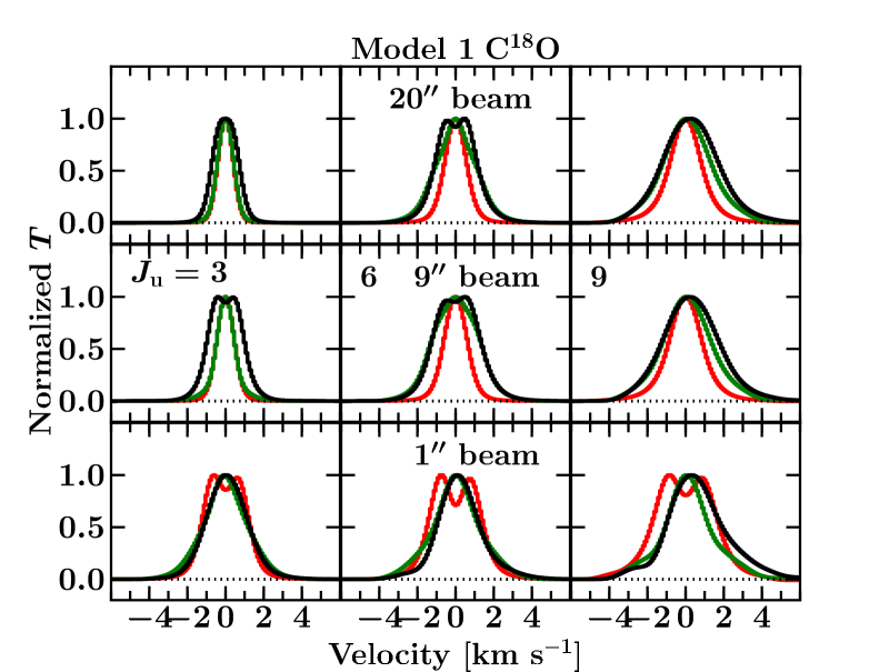
Figure 3: Normalized C¹⁸O line profiles as functions of evolution for $J_{\mathrm{u}}=3$, 6 and 9 at $t/t_{\mathrm{acc}}=0.13$ (red), 0.50 (green) and 0.96 (black) for $i=5^{\circ}$ orientation for Model 1. The lines are convolved to beams of 20$\arcsec$ (top), 9$\arcsec$ (middle) and 1$\arcsec$ (bottom).

The first time step used for the molecular line simulation is at $t=1000$ years ($t/t_{\rm acc}\sim 10^{-3}$), where the central heating is not yet turned on. The evolution of the mass and the effective temperature is shown in the Appendix B. The effective temperature during this time step is 10 K and the models are still spherically symmetric. The TSC84 velocity profile for this time step reaches a maximum radial component of 10 km s^-1 at 0.1 AU. However, CO is frozen out in the inner envelope, so the FIR and submm lines (populated up to $J_{\rm u}\leq 8$) show neither wing emission nor blue asymmetry as typical signposts of an infalling envelope. Instead, the CO lines probe the static outer envelope at this point, where the low density has prevented CO from freezing out.

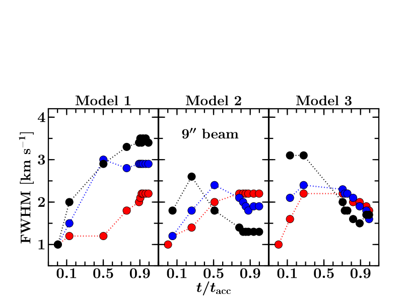
Figure 4: C¹⁸O 3-2 (red), 6-5 (blue) and 9-8 (black) FWHM evolution within a 9$\arcsec$ beam for the 3 different models at $i=5^{\circ}$ orientation.

The line profiles change shape once the effective source temperature increases to above a few thousand K at $t>10^{4}$ yr (see Fig. 3 and Appendix B for the line profile evolution). The line profiles become more asymmetric (Fig. 18) toward higher excitation and smaller beams, because in both cases a larger contribution from warm, infalling gas in the inner envelope and optical depth affect the emission lines. The line widths are due to a combination of thermal broadening, turbulent width and velocity structure, but examination of models without a systematic velocity field confirm that the increase in broadening is mostly due to infall (see also Lee et al. 2004). Models 2 and 3 show narrower lines during Stage I ($t/t_{\rm acc}\geq 0.5$) since they are relatively more rotationally dominated than in Model 1. As shown in Fig. 4, the higher-$J$ ($J_{\rm u}\geq 5$) lines are broadened significantly during Stage 0.

The line profiles in a 1$\arcsec$ beam depend strongly on the velocity field on small scales and show more structure than the line profiles in the larger beams (Figs. 3 and 20). The lines in a 1$\arcsec$ beam are broader and show multiple velocity components (in particular for ¹²CO and ¹³CO) reflecting the complex dynamics due to infall and rotation plus the effects of optical depth and high angular resolution. A combination of CO isotopolog lines can provide a powerful diagnostic of the velocity and density structure on $10-1000$ AU scales (see also §3.4).

In summary, the infalling gas can significantly broaden the optically thin gas as shown in Fig. 4. The velocity profile in the inner envelope affects the broadening of the high-$J$ ($J_{\rm u}>6$) line. These lines can be a powerful diagnostic of the velocity and density structure in the inner 1000 AU ($\leq 9\arcsec$ beams).

3.2 CO rotational temperature

The observed integrated intensities (K km s^-1) are commonly analyzed by constructing a Boltzmann diagram and calculating the associated rotational temperature. Another useful representation is to plot the integrated flux ($\int F_{\nu}d\nu$ in W m^-2) as a function of upper level rotational quantum number (spectral line energy distribution or SLED) to determine the $J$ level at which the peak of the molecular emission occurs. The conversion between integrated intensities and integrated flux is given by

$$\int F_{\nu}d\nu=\frac{2k}{\lambda^{3}}d\Omega\int T_{v}dv.$$ (1)

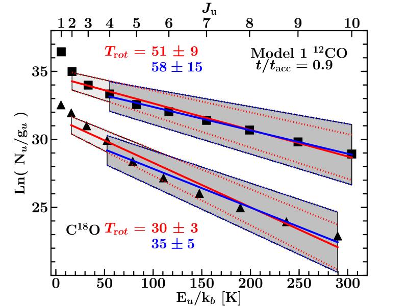
Figure 5: Examples of single-temperature fits through the ¹²CO (squares) and C¹⁸O (triangles) lines obtained from Model 1 fluxes at $t/t_{\rm acc}=0.9$ in a 9^′′ beam. The red line shows the linear fit from $J_{\rm u}=2$ up to $J_{\mathrm{u}}=10$ while the blue line is the fit up starting from $J_{\rm u}=4$ up to $J_{\rm u}=10$. The gray shaded regions indicate one standard deviation from the best fit.

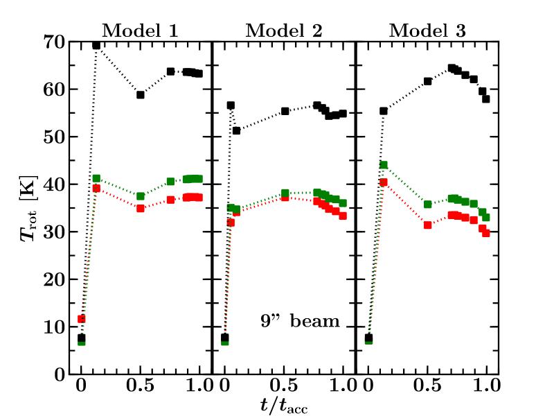
Figure 6: Evolution of the rotational temperature ($T_{\mathrm{rot}}$) from a single-temperature fit through $J_{\mathrm{u}}=2-10$. The different colors are for different isotopologs: ¹²CO (black), ¹³CO (green) and C¹⁸O (blue). The typical errors are 15, 5 and 3 K for ¹²CO, ¹³CO and C¹⁸O, respectively. The different panels show the results for different models as indicated.

Examples of single-temperature fits through the modeled lines are shown in Fig. 5 for Model 1. Observationally, temperatures are generally measured from $J_{\rm u}=2$ to 10 (Yıldız et al. 2012, 2013) and from 4 to 10 (Goicoechea et al. 2012). The evolution of the rotational temperatures within a 9$\arcsec$ beam is shown in Fig. 6 for the three models. At very early times, $t/t_{\rm acc}<0.1$, a single excitation temperature of $\sim$ 8–12 K characterizes the CO Boltzmann diagrams. After the central source turns on, the excitation temperature is nearly constant with time. In a beam of 9$\arcsec$, most of the flux up to $J_{\rm u}=10$ comes from the $>$ 100 AU region, which is not necessarily the $>100$ K gas (Yıldız et al. 2010) even for face-on orientation. Therefore, within $\geq 9\arcsec$ beams, the observed emission is not sensitive to the warming up of material as the system evolves.

A value of 46 to 65 K characterizes the ¹²CO distribution for all models. However, ¹²CO is optically thick, which drives the temperature to higher values due to under-estimated low-$J$ column densities. The C¹⁸O and ¹³CO distributions are fitted with similar excitation temperatures between 29 and 42 K within a 9$\arcsec$ beam. Because Model 3 has a higher inner envelope density, the derived rotational temperature at the second time step is relatively high ($\gtrsim$ 40 K) due to an optical depth effect.

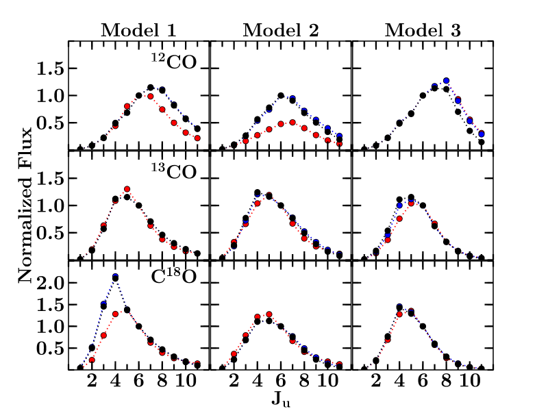
Figure 7: Evolution of normalized CO spectral line energy distribution (SLED) in a 9$\arcsec$ beam. The CO integrated fluxes (W m^-2) are normalized to $J_{\mathrm{u}}=6$. The different colors indicate different times: $t/t_{\mathrm{acc}}\sim 0.50$ (red), 0.75 (blue), 0.96 (black).

The integrated fluxes can also be used to construct CO SLEDs. The ¹²CO SLED peaks at $J_{\mathrm{u}}=6-8$ with small dependence on the heating luminosity (Fig. 7). The peak of the SLED does not depend on the beam size for beams $\geq 9{\arcsec}$. The same applies to the ¹³CO and C¹⁸O SLEDs which peak at $J_{\mathrm{u}}=4-5$. There is no significant observable evolution in the SLEDs once the star is turned on. A passively heated system is characterized by such SLEDs regardless of the evolutionary state as long as the heating luminosity is $\sim 1-10$ $L_{\odot}$ ($T_{\star}\sim$ 1000–4500 K).

The picture within a 1$\arcsec$ beam is different since it resolves the inner envelope. The best-fit single temperature component depends on whether or not the disk fills a significant fraction of the beam. If it does (Models 2 and 3), the C¹⁸O and ¹³CO rotational temperatures are $\sim$40–50 K. There is less spread than within the 9$\arcsec$ beam due to the higher densities bringing the excitation closer to LTE. Without a significant disk contribution in a $1\arcsec$ beam (Model 1), the ¹³CO excitation temperature is closer to 60 K while that of C¹⁸O is similar to the other models at $\sim 40$ K. The ¹²CO rotational temperature is $T_{\rm rot}\simeq 70$ K in all of the models. Furthermore, the CO SLED within a 1$\arcsec$ beam peaks at $J_{\rm u}=6,8$ and $10$ for C¹⁸O, ¹³CO and ¹²CO, respectively.

A comparison with the sample presented in Yıldız et al. (2013) indicates that the lack of $T_{\rm rot}$ evolution is consistent with observations, and our predicted values for $T_{\rm rot}$ match the data. On the other hand, the observed ¹³CO $T_{\rm rot}$ and SLED are generally higher than predicted, which suggests an additional heating component is needed to excite the ¹³CO lines. A more detailed comparison between model prediction and observation can be found in Yıldız et al. (2013).

In summary, both rotational temperatures derived from Boltzmann diagrams and CO SLEDs of passively heated systems do not evolve with time once the star is turned on. Optically thin ¹³CO and C¹⁸O lines are characterized by single excitation temperatures of the order 30–40 K within a wide range of beams ($\geq 9\arcsec$). The CO SLED peaks at $J_{\mathrm{u}}=7\pm 1$ and $J_{\mathrm{u}}=4-5$ for ¹²CO and other isotopologs, respectively. In $1\arcsec$ beam, the peak of the SLED shifts upward by $\sim 2$ $J$ levels and a warmer rotational temperature by 10 K in the presence of a disk.

3.3 Disk contribution to line fluxes

After deriving a number of observables, an important question is, what the fraction of the flux contributed by the disk is? This contribution can be calculated from the averaged (over line profile and direction) escape probability of the line emission $\eta_{\rm ul}$, which is the probability that a photon escapes both the dust and line absorption (Takahashi et al. 1983; Bruderer et al. 2012). The escape probabilities are used to calculate the cooling rate, $\Gamma_{\rm cool,\nu}$, of each computational cell and each transition with the following formula

$$\Gamma_{\rm cool,\nu}=\frac{V}{4\pi}h\nu_{\rm ul}A_{\rm ul}nx_{\rm u}\eta_{\rm ul},$$ (2)

where $\nu_{\rm ul}$ is the frequency of the line, $A_{\rm ul}$ is the Einstein $A$ coefficient, $x_{\rm u}$ is the normalized population level and $n$ is the density of the molecule. The disk contribution is then the ratio of the sum of cooling rates from the cells in the disk compared to the cells within a Gaussian beam. The cooling rates are weighted with a Gaussian beam of size 9$\arcsec$ or 1$\arcsec$ while the disk emitting region is defined as shown in Fig. 2. The flux is then given through an integration of line of sight, $F_{\nu}=\int\Gamma_{\rm cool,\nu}ds_{\rm LOS}$, which translates into the same constant factor in both disk and total fluxes.

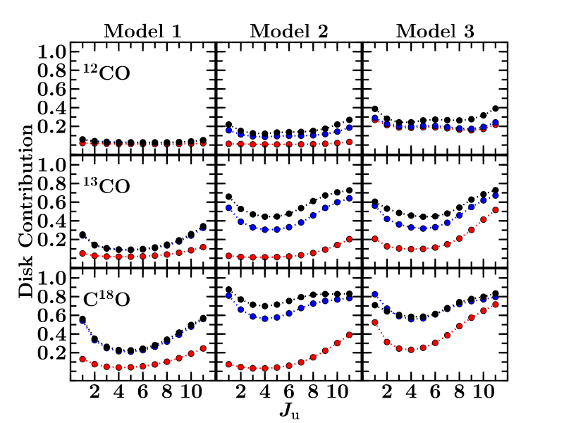
Figure 8: Disk contribution as a function of $J_{\mathrm{u}}$ within 1${\arcsec}$ (140 AU at 140 pc) for the three different models. The different colors correspond to different evolutionary stages: $t/t_{\mathrm{acc}}\sim 0.50$ (red, $M_{\rm env}/M_{\rm disk}\geq 3$), 0.75 (blue, $M_{\rm env}/M_{\rm disk}\sim 1$), 0.96 (black, $M_{\rm env}/M_{\rm disk}<1$).

For a single-dish 9$\arcsec$ beam, one needs to go to higher rotational transitions with $J_{\mathrm{u}}>6$ at later stages to obtain a $>$ 50% disk contribution, if the disk can be detected at all (Fig. 21). The disk is difficult to observe directly in ¹²CO and ¹³CO emission since the lines quickly become optically thick unless lines with $J_{\rm u}>10$ are observed. A larger disk contribution is seen in the optically thin C¹⁸O lines, but here the low absolute flux may become prohibitive.

For example, the expected C¹⁸O disk fluxes for $J_{\rm u}>14$ within the PACS wavelength range are $\leq 10^{-20}$ W m^-2 which will take $>100$ hours to detect with PACS. Herschel-HIFI is able to spectrally resolved the C¹⁸O $J_{\rm u}=10$ and 9 lines but has a $\sim 20$″ beam, which lowers the disk fraction by a factor of 2 relative to a 9$\arcsec$ beam. Peak temperatures of only 1–8 mK during Stage 0 and 2–12 mK in Stage I phase are expected, which are readily overwhelmed by the envelope emission. The spectrally resolved C¹⁸O spectra observed with HIFI indeed do not show any sign of disk emission, consistent with our predictions (San Jose-Garcia et al. 2013; Yıldız et al. 2012, 2013).

A more interesting result is the disk contribution to the CO lines within a 1^′′ (140 AU) region as shown in Fig. 8. The simulations suggest a significant disk contribution ($>$ 50%) for the ¹³CO and C¹⁸O lines within this scale, even for the $J=1-0$ transition. For Model 3, the high disk contribution is expected to happen before the system enters Stage 1 ($M_{\mathrm{env}}\leq M_{\star}$): a significant disk contribution is seen even at $t/t_{\mathrm{acc}}=0.3$. However, Model 2 shows a significant disk contribution only in the second half of the accretion phase. Model 2 shows a significant jump in the disk contribution between $t/t_{\rm acc}=0.5$ and 0.75 which is due to significant contribution from the flattened inner envelope within 1$\arcsec$ at $t/t_{\rm acc}=0.5$. Thus, the relatively more optically thin CO isotopolog emission is dominated by the central rotating disk starting from the Stage 1 phase ($t/t_{\rm acc}\geq 0.5$).

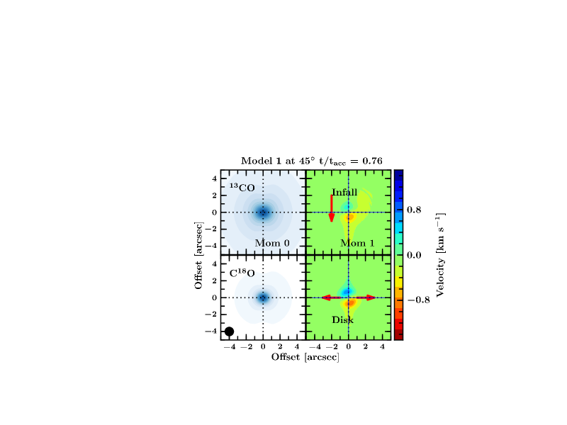
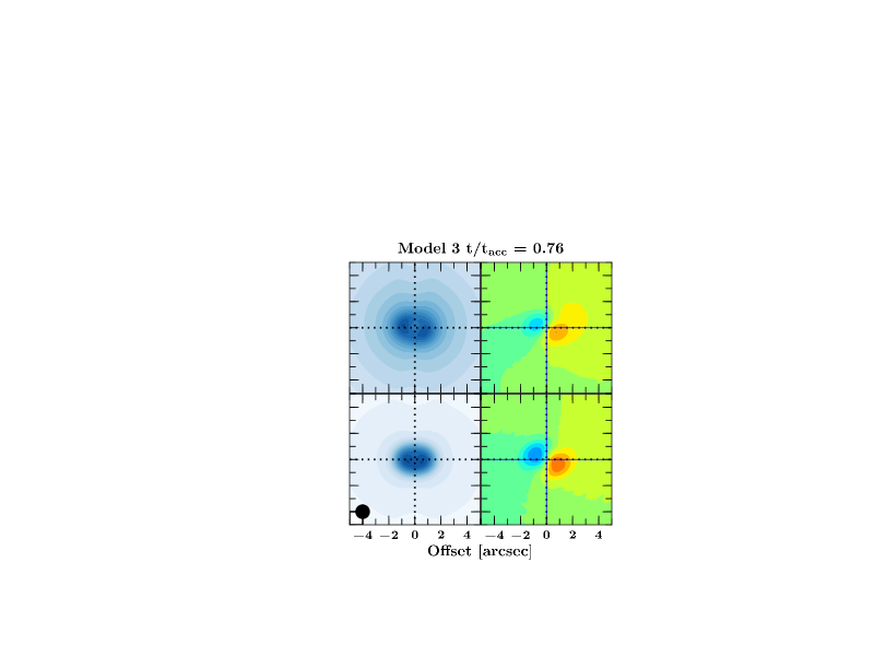
Figure 9: ¹³CO and C¹⁸O zeroth (left panels) and first (right panels) moment maps for Model 1 and 3 at 45^∘ inclination at a resolution of 1$\arcsec$. The red arrows indicate the direction of infall and rotationally supported disk. The velocity scale is given on the right-hand side of the left figure.

3.4 Disentangling the velocity field

How can the rotating and infalling flattened envelope be disentangled from the Keplerian motion of the disk? The evolution of the rotationally dominated region is consistent with that reported by Brinch et al. (2008) based on more detailed hydrodynamics simulations. All models become rotationally dominated within 500 AU at $t/t_{\rm acc}>0.3$.

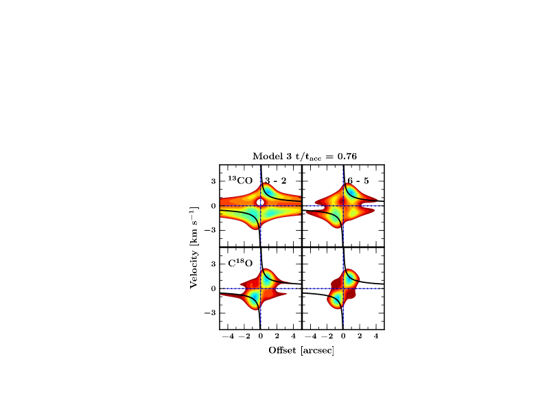
Figure 10: Position-velocity slice for the ¹³CO and C¹⁸O $J_{\rm u}=3$ and $J_{\rm u}=6$ transitions along the major axis of the zeroth moment map. The solid black lines are the Keplerian velocity structure calculated from the stellar mass.

The presence of an embedded disk can be inferred from the presence of elongated ¹³CO and C¹⁸O integrated intensity maps (moment 0 of Fig. 9) coupled with the moment 1 map. In the presence of a stable disk, the zeroth moment map is elongated perpendicular to the outflow axis with a double peaked structure. This feature is not seen in Model 1 (Fig. 9 left) since the disk is much smaller than the 1$\arcsec$ beam. In the case of Model 3, the relatively massive disk exhibits a double peaked zeroth moment map which is perpendicular to the outflow direction.

A velocity gradient is seen in the moment 1 maps for both Models 1 and 3. With the high resolution of the modeled spectra, it is possible to differentiate between the disk and envelope (Hogerheijde 2001). The presence of a velocity gradient along the major axis of the elongation in the moment 1 map is a clear sign of a stable embedded disk in the case of Model 3. In addition, from the analysis in Sect. 3.3, we can also attribute the bulk of optically thin emission in Model 3 to the disk. Meanwhile, the infalling rotating envelope contribution can be detected through the fact that the moment 1 map is not perfectly aligned but skewed. On the other hand, a velocity gradient without the presence of elongation in the zeroth moment map such as in Model 1 (Fig. 9) indicates an infalling envelope.

Position-velocity (PV) diagrams provide another way to study the velocity structure. Figure 10 shows PV slices following the direction of the major axis of the disk (PA = 90^∘) in the integrated intensity map in the 3–2 and 6–5 lines. A simple way to analyze PV diagrams is to separate the diagram into four quadrants and examine which quadrants have considerable emission. An infall dominated PV diagram without rotation is symmetric about the velocity axis with all four quadrants filled (Ohashi et al. 1997). The presence of rotation breaks the symmetry in the PV diagram and causes the peak positions to be off-centered. As found previously in hydrodynamical simulations by Brinch et al. (2008), infall dominates the PV diagrams at early times while rotation dominates the later times. These features have been observed toward low-mass YSOs which suggests that generally the infalling rotating envelope dominates the PV diagrams (eg. Sargent & Beckwith 1987; Hayashi et al. 1993; Saito et al. 1996; Ohashi et al. 1997; Hogerheijde 2001).

Focusing on Model 3 at $t/t_{\rm acc}=0.76$ (near the end of Stage I) as shown in Fig. 10, the C¹⁸O PV diagrams show a clearer pure rotation dominated structure than the ¹³CO lines. They can thus be used to constrain the stellar mass as long as the inclination is known. Also, the higher-$J$ lines provide a better view into the rotating structure and should give tighter constraints on the stellar mass.

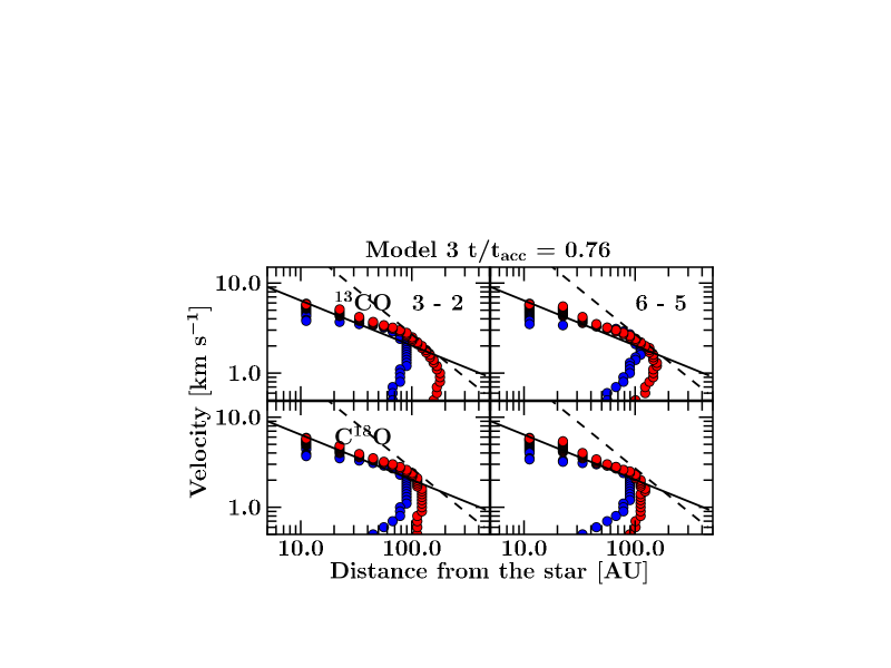
Figure 11: Velocity as function of distance of the peak intensity position from the protostar, as measured in each channel map and for the same transitions as in Fig. 10. The red and blue colors represent the red- and blue-shifted components. The solid black line indicates the expected Keplerian structure from the stellar mass in the model, where as the dashed lines indicate the $v\propto R^{-1}$ relation as a comparison.

Another method is to plot the velocity as function of distance of the position of the peak intensity (Sargent & Beckwith 1987). This is done for the red-shifted and blue-shifted components, plotted in Fig. 11. The method is similar to the spectroastrometry technique employed in the optical and NIR observations (Takami et al. 2001; Baines et al. 2006; Pontoppidan et al. 2008). A Keplerian disk is characterized by a $v\propto r^{-0.5}$ with large contribution from the high velocity gas which is optically thin. As noted by Sargent & Beckwith (1987), as long as the line is spectrally resolved ($dV=0.1$km s^-1), the peak position corresponds to the maximum radius of a given velocity. On the other hand, the emission at low velocities ($dV\sim V$) is relatively more optically thick and is dominated by the infalling rotating envelope which peaks closer to the center (no offset). Such an analysis can be performed directly from the interferometric data and is a powerful tool in searching for embedded rotationally stable disks out of the rotating infalling envelope.

Why is there a difference between the red-shifted and blue-shifted components in Fig. 11? At high velocities, this is due to unresolved emission hence the different velocity components simply peak at the same position and the difference reflects the uncertainty in locating the emitting region. At low velocities, the optically thick infalling rotating envelope affects the peak positions. In an infalling envelope, the blue-shifted emission is relatively more optically thin than the red-shifted emission (Evans 1999). Such difference in the optical depth causes the red- and blue-shifted emissions to be asymmetric as found in the moment 1 map.

4 NIR CO absorption lines

A complementary probe of the molecular excitation conditions is provided by the NIR CO ro-vibrational absorption lines. In this work, we concentrate on the $\mathrm{v}=1-0$ band at 4.76 $\mu$m. This absorption takes place along the line of sight through the envelope and/or disk up to where the continuum is formed. The absorption lines are therefore computed for different inclinations of 45^∘ and 75^∘. The inclinations were chosen such that they probe the envelope ($>15^{\circ}$) and the part of the disk that is not completely optically thick such that there is enough observable NIR continuum ($\leq 75^{\circ}$), i.e., lines of sight that graze the disk atmosphere. Since our focus is on the excitation, the absorption lines have been calculated without any velocity field besides a turbulent width (Doppler $b$) of 0.8 km s^-1. More importantly, the formation of the 4.7$\mu$m continuum is strongly dependent on the inclination which affect the molecular absorption lines.

4.1 Evolution of NIR absorption spectra

4.1.1 Radiative transfer and non-LTE effects

The line center optical depth is one of the quantities derived from the model that can be compared to observations. This optical depth can either be determined by computing the line of sight integrated column densities and converting this to optical depth or by using a full RADLite calculation. For both approaches, the same level populations are used, i.e., the same model for the CO excitation is adopted as in Section 3. In the simplest method, the line center optical depth is obtained from

$$\tau_{0}=\frac{c^{3}g_{\mathrm{u}}}{8\pi\sqrt{\pi}b\nu^{3}g_{\mathrm{l}}}A_{\mathrm{ul}}N_{\mathrm{l}},$$ (3)

where $\nu$ is the line frequency and $N_{\mathrm{l}}$ is the lower level column density along the line of sight. The main difference between the methods is that RADLite solves the radiative transfer equation along the line of sight and thus accounts for continuum and line optical depth effects and scattered continuum photons, while such effects are not considered in the column density approach. In addition, RADLite accounts for the continuum formation, while a ray through the center does not. Thus, the two methods effectively compare the total mass present along a ray and the observed mass as probed by the line optical depth returned by RADLite. The optical depth is extracted from the RADLite spectra using the line-to-continuum ratio at the line center.

As discussed and illustrated extensively in Appendix C.1, the two approaches can give very different results, especially for the higher $J$ lines for which the line optical depths can differ by more than an order of magnitude. The main reason is illustrated in Fig. 24, which shows the region where the NIR continuum arises. For small inclinations, the continuum is essentially point-like, but for higher inclinations larger radii contribute significantly and the continuum is no longer a point source. Thus, for high inclinations, the high-$J$ lines start absorbing off-center, away from warm gas in the inner few AU that are included in the column method. The location of the continuum is typically at $>$10 AU at $i=75^{\circ}$ which results in two to three orders of magnitude difference in total column density. For the case of $i\sim 45^{\circ}$, the result depends on the physical structure in the inner few AU but the absorption can miss the warm high density region close to the midplane of the disk where most of the $J\geq 10$ is located (Fig. 23).

Figure 26 and 27 also compare LTE and non-LTE spectra. Consistent with Section 3, significant differences are found for the higher pure rotational levels which are subthermally excited. However, the radiative transfer effect is generally more important than the non-LTE effects for viewing angles through the disk/inner envelope surface.

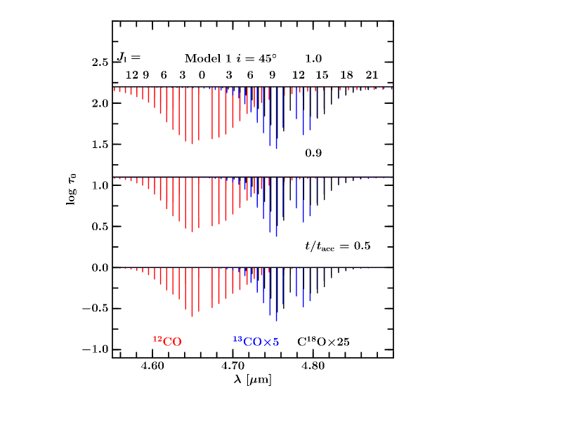
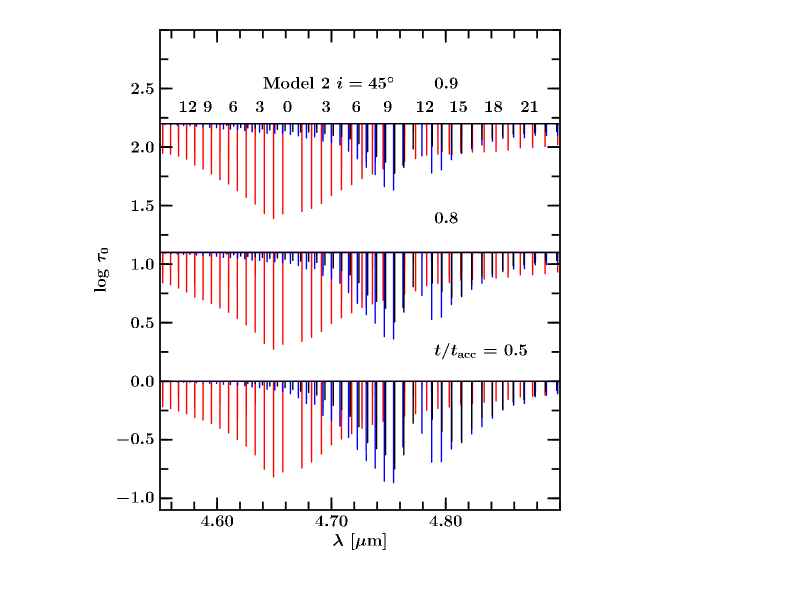
Figure 12: Evolution of the ¹²CO (red), ¹³CO (blue) and C¹⁸O (black) absorption lines for Model 1 at $i=45^{\circ}$. The evolution of the absorption lines for Model 2 is shown at the bottom panel. The lower rotational levels are indicated on top of the first spectrum. All of the ¹³CO lines are multiplied by 5 and C¹⁸O lines by 25.

4.1.2 NIR spectra

The NIR absorptions are rendered with RADLite for $t/t_{\rm acc}\geq 0.5$ which starts when $M_{\rm env}\sim M_{\star}$ (Stage 0/I boundary) in order to have a strong 4.7$\mu$m continuum. Figure 12 show the P and R branches of the CO isotopologs for Model 1 and 2 which show the greatest difference. In general, as shown in Fig. 12, the higher-$J$ absorptions are stronger as the system evolves into Stage II due to the central luminosity. For Model 1, at $t/t_{\rm acc}=0.5$, the ¹²CO absorptions can be seen up to $J=16$, and up to $J=9$ for ¹³CO and 7 for C¹⁸O. The number of absorption lines that are above $\tau_{\nu}=3\times 10^{-3}$ (the 3$\sigma$ observational limit with instruments such as VLT-CRIRES) doubles at the end of the accretion phase and the highest observable $J$ shifts from 16 to $>30$ for ¹²CO and up to $\sim$ 15–20 for the isotopologs.

At early times, a similar number of lines are found for Model 3 but their optical depths are lower due to the difference in the inner envelope structure. On the other hand, the number of lines in Model 2 is much higher than in the other two models due to the lower continuum optical depth in the inner envelope. Thus, the absorbing column starts deeper than in the other two models, which results in stronger absorption features and an increased number of detectable high-$J$ lines, up to $J>40$ for ¹²CO, $J\sim 25$ for ¹³CO and $J\sim 15$ for C¹⁸O (Fig. 12). Thus, in principle the appearance of the NIR spectrum could be a sensitive probe of the inner envelope structure. In practice, the ¹²CO absorption will be affected by outflows and winds so the ¹³CO and C¹⁸O isotopologs are most useful for this purpose.

4.2 Rotational temperatures

A directly related observable is the rotational temperature derived from a Boltzmann diagram. Thus, the RADLite NIR spectra need to be converted into column densities. For this conversion, we use a standard curve-of-growth analysis (Spitzer 1989) with $b=0.8$ km s^-1 and oscillator strengths derived from the Einstein $A_{\rm ul}$ coefficients. By using the curve-of-growth method, it is assumed that the spectral lines are unresolved.

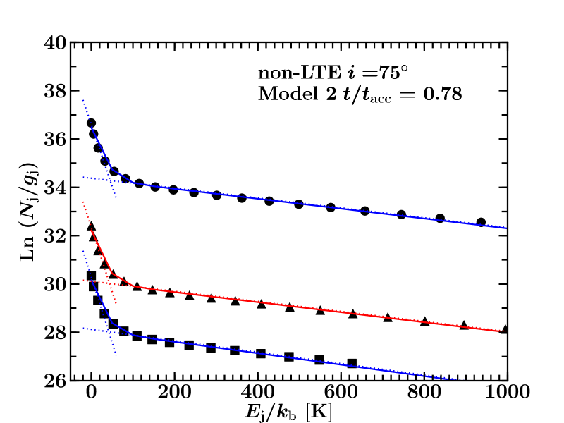
Figure 22: Example of the two-temperature fitting of the NIR lines. The column densities are derived from a curve-of-growth analysis performed on the simulated spectra using RADLite. The different symbols correspond to ¹²CO (circle), ¹³CO (triangles) and C¹⁸O (squares). The solid lines are the combination of the cold and warm components.

An example of a Boltzmann diagram is shown in Fig. 22 together with a two-temperature fit, as commonly done in observations (Mitchell et al. 1990; Smith et al. 2009; Herczeg et al. 2011). The rotational temperature of the cold component is obtained from fitting the P(1) to P(4) lines ($E_{\mathrm{l}}<40$ K). Lines higher than P(5) ($E_{\mathrm{l}}>40$ K) are used to obtain the temperature of the warm component. Model 2 at $t/t_{\rm acc}=0.78$ is used since it clearly shows the break between the two temperatures.

How do the two temperatures evolve with time? As Table 2 shows, the cold component is between 20 and 35 K with no significant evolution, except in Model 2, as the disk is building up. The warm component, however, increases with inclination and time. The derived warm temperature component ranges from $<100$ up to $\sim 520$ K and traces the warming up of material in the inner region as the envelope dissipates. From the simulations, a $>400$ K warm component is a signature of an evolved system.

Table 2: NIR rotational temperatures derived from $\tau_{0}>10^{-3}$ lines for $i=45^{\circ}$ and 75^∘.

		12CO		13CO		C18O
$t/t_{\mathrm{acc}}$	$i$	$T_{\mathrm{cold}}$	$T_{\mathrm{warm}}$	$T_{\mathrm{cold}}$	$T_{\mathrm{warm}}$	$T_{\mathrm{cold}}$	$T_{\mathrm{warm}}$
	[∘]	[K]	[K]	[K]	[K]	[K]	[K]
Model 1
0.50	45	$21\pm 9$	$80\pm 9$	$18\pm 11$	$49\pm 18$	$19\pm 13$	…
	75	$20\pm 9$	$66\pm 8$	$17\pm 10$	$44\pm 10$	$18\pm 10$	…
0.76	45	$26\pm 10$	$142\pm 21$	$19\pm 11$	$72\pm 20$	$19\pm 14$	…
	75	$25\pm 12$	$260\pm 67$	$25\pm 12$	$273\pm 69$	$19\pm 13$	…
0.96	45	$28\pm 10$	$201\pm 36$	$28\pm 13$	$207\pm 46$	$21\pm 16$	…
	75	$25\pm 10$	$271\pm 61$	$25\pm 13$	$301\pm 80$	$20\pm 13$	…
Model 2
0.50	45	$34\pm 20$	$245\pm 61$	$34\pm 25$	$253\pm 61$	$29\pm 23$	$183\pm 51$
	75	$31\pm 20$	$293\pm 85$	$31\pm 20$	$302\pm 86$	$27\pm 19$	$209\pm 67$
0.78	45	$31\pm 20$	$327\pm 100$	$31\pm 20$	$340\pm 110$	$28\pm 19$	$264\pm 89$
	75	$20\pm 11$	$489\pm 210$	$19\pm 11$	$481\pm 192$	$18\pm 11$	$423\pm 230$
0.94	45	$28\pm 18$	$402\pm 156$	$28\pm 18$	$410\pm 152$	$26\pm 17$	$333\pm 139$
	75	$18\pm 11$	$544\pm 255$	$17\pm 10$	$527\pm 223$	$17\pm 10$	$495\pm 308$
Model 3
0.50	45	$21\pm 6$	$193\pm 37$	$16\pm 8$	$42\pm 21$	$19\pm 9$	…
	75	$16\pm 7$	$37\pm 7$	$16\pm 10$	…	$16\pm 11$	…
0.76	45	$23\pm 9$	$287\pm 80$	$22\pm 9$	$304\pm 85$	$17\pm 11$	…
	75	$22\pm 8$	$289\pm 81$	$21\pm 8$	$302\pm 83$	$17\pm 10$	…
0.96	45	$22\pm 9$	$366\pm 128$	$21\pm 8$	$381\pm 129$	$17\pm 10$	…
	75	$18\pm 8$	$361\pm 121$	$18\pm 7$	$371\pm 119$	$16\pm 9$	…

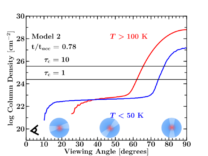
Figure 13: Integrated gas column density along the different viewing angles for Model 2. The red and blues lines indicate the warm ($T>100$ K) and cold gas ($T<50$ K), respectively. The approximate continuum optical depths, $\tau_{\rm c}=1$ and 10, are also shown to indicate the amount material that is missed by properly solving the radiative transfer equation.

What is the origin of the two temperatures? This can be easily shown by plotting the cold ($<$50 K) and warm ($>$100 K) H₂ column along the line of sight at various inclinations (Fig. 13). The particular model and time were chosen as an example; the general picture is the same independent of evolutionary model, but the warm component shifts to lower viewing angle (left) for earlier times. The figure indicates that the warm material can be probed through $i>25^{\circ}$ viewing angles. The cold component probes the outer envelope where the gas temperature hardly changes as the system evolves. The warm component reflects the line of sight to the center through the warm inner envelope (the so-called ‘hot core’ ) or the disk surface where the gas is $>100$ K in all of our models. The cumulative gas column density indicates that the cold material is mostly absorbed at $R>100$ AU while the warmer gas component is probing the inner few AU ($i>60^{\circ}$) up to $\sim$20 AU ($i\sim 45^{\circ}$). The excitation temperature of the warm component reflects the density structure in the inner few AU. With the lower densities and warmer temperatures in Model 2, which decreases the effective continuum optical depth, higher warm temperatures can be observed as the absorption probes deeper to smaller radii than the other two models.

5 Discussion

We have presented the evolution of CO molecular lines based on the standard picture of a prestellar core collapsing to form a star and 2D circumstellar disk. The main aim of this work is to study the evolution of observables that are derived from the spectra such as rotational temperatures, line profiles, and velocity fields. Specifically, signatures of disk formation during the embedded stage that can be obtained with the most commonly used molecule, CO, are investigated.

5.1 Detecting disk signatures in the embedded phase

How can one determine whether disks have formed in the earliest Stage 0? As discussed in Section 3.3, it is difficult to isolate an embedded disk component in single-dish observations. The disk contribution to the observed flux within $>9\arcsec$ beams is only significant ($>$60%) for the ¹³CO and C¹⁸O $J_{\rm u}>9$ lines at $t/t_{\rm acc}>0.75$. However, the absolute fluxes are too low to be detected. Thus, spatially resolved observations at sub-arcsec scale are needed.

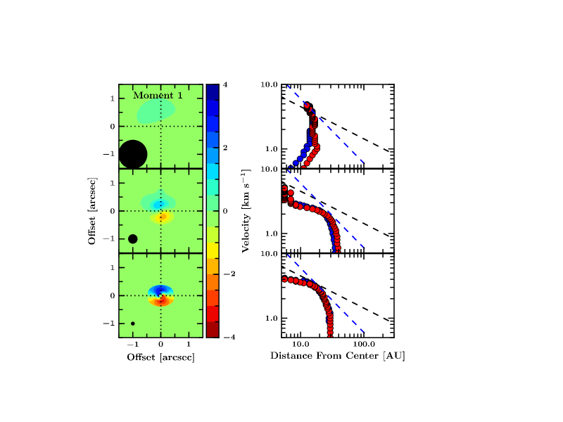
Figure 14: C¹⁸O 3–2 moment-one (left) and spectroastrometry (right) for Model 1 at the end of Stage 0 convolved to a 1$\arcsec$ (top), 0.3$\arcsec$ (middle) and 0.1$\arcsec$ (bottom) as shown by the solid circle. The Keplerian structure at this stage extends up to 20 AU (0.14$\arcsec$ radius). The black dashed line in the right panel shows the $v\propto R^{-0.5}$ and the blue dashed line indicates the $v\propto R^{-1}$ relation.

What are the signatures of an embedded rotationally supported disk on subarcsecond scales? We have analyzed some of the simulated images during the Stage 0 phase at a resolution of 0.1$\arcsec$ as can readily be observed with ALMA. Figure 14 shows the C¹⁸O 3–2 moment-one map during the Stage 0 phase of Model 1 with a disk extending up to 20 AU at a resolution of 1, 0.3 and 0.1$\arcsec$. Velocity gradients are present in all of the moment-one maps although it is weaker within a 1$\arcsec$ beam. The right panel of the figure shows the spectroastrometry (Fig. 11) within the different resolutions. The velocity gradient within a 0.5–1$\arcsec$ beam exhibits a $v\propto R^{-1}$ relation since the inner envelope dominates the emission. Within the smaller beams, the velocity gradient is resolved into two components: $v\propto R^{-1}$ (blue dashed line) due to envelope and $v\propto R^{-0.5}$ (black dashed line) due to the stable disk. A $v\propto R^{-0.5}$ can be seen when the disk is marginally resolved, however, the derived stellar mass is far below the real stellar mass. It is very important that the disk is fully resolved in order to derive the stellar mass. With the C¹⁸O lines, a resolved embedded disk in Stage 0 would have the following features:

• Elongated moment-zero map.

• A transition between an infalling envelope to a rotating disk: a skewed moment-one map.

• The Keplerian structure exhibits a clear $v\propto R^{-0.5}$ (Fig. 11 and bottom of Fig. 14 ) velocity gradient perpendicular to the outflow.

It is possible to search for rotationally supported disks in Stage 0 sources with characteristics of Model 1 with the full ALMA array in less than 30 minutes for the C¹⁸O 2–1 transition or up to 4 hours for the 6–5 transition. For Models 2 and 3, the disks have grown up to $\sim 50$ AU near the end of Stage 0 and up to twice more massive, thus it will take less than 2 hours to observe them with ALMA in the 6–5 transition and less than 30 minutes in the 2–1 and 3–2 transitions. Therefore, ALMA will allow us, for the first time, to test whether rotationally supported disks have grown beyond 10 AU by the end of the Stage 0 phase.

The question of when rotationally supported disks form is crucial to the physical and chemical evolution of accretion disks. In our evolutionary models, the disks have radii up to 50 AU at the end of Stage 0 phase and can be as small as 20 AU. Dapp & Basu (2010) and Dapp et al. (2012) numerically showed that disks do not grow beyond 10 AU during the Stage 0 phase in the presence of magnetic fields due to the magnetic breaking problem (see also Li et al. 2011; Joos et al. 2012). This is consistent with the lack of observed rotationally supported disks toward Stage 0 objects so far (Brinch et al. 2009; Maury et al. 2010). On the other hand, there is a growing body of observational evidence for rotating disks in Stage I YSOs (Brinch et al. 2007; Lommen et al. 2008; Jørgensen et al. 2009; Takakuwa et al. 2012). The size of the rotationally supported disk depends on the initial parameters of the collapsing envelope. In our models, the sizes of Models 2 and 3 are consistent with the observed Keplerian velocity structure in Stage I sources (Jørgensen et al. 2009).

An additional caveat is that our models lead to a Keplerian disk with a flattened inner envelope on similar scales as the stable disk. Hydrodynamical simulations, on the other hand, show a stable disk embedded in a much larger rotating flattened structure and with more turbulent structure (Brinch et al. 2008; Kratter et al. 2010). Furthermore, the 3D simulations by Harsono et al. (2011) suggest that 50% of the embedded disk is sub-Keplerian due to interaction with the envelope. The predicted moment 1 maps and spectroastrometry with the current models should be performed for these numerical simulations for comparison with ALMA observations.

5.2 Probing the temperature structure

The derived rotational temperatures from the submm and FIR lines ($J_{\rm u}$ = 1–10) within $>9\arcsec$ beams do not evolve with time, in contrast with the continuum SED, and largely trace the outer envelope (Section 3.2). Even though the disk structure is hotter with time, the emission that comes from within that region is much smaller than the beam. The mass weighted temperature of the system which contributes to the overall emission is constant with time. The rotational temperatures also cannot differentiate between the three different evolutionary models. In addition, the peak of the CO SLED is constant throughout the evolution at $J_{\rm u}=4$ for the ¹³CO and C¹⁸O. The higher observed excitation temperatures for ¹²CO and ¹³CO in a wide range of low-mass protostars from submm and FIR data point to other physical processes that are present in the system such as UV heating and C-shock components that affect the $J\geq 5$ lines (Visser et al. 2012; Yıldız et al. 2012).

The NIR absorption lines toward embedded YSOs are complementary to the submm/FIR rotational lines. Both techniques probe the bulk of the cold envelope, but the NIR lines also probe the warm component because the lines start absorbing at the $\tau\sim 1$ surface deep inside the inner envelope. Consequently, the cold component present in the NIR lines should be similar to the component observed in the submm. Indeed, the typical rotational temperatures of 20–30 K found in the NIR models for C¹⁸O are comparable to the values of 30–40 K found from the submm simulations.

The warm up process is accessible through NIR molecular absorption lines. In Section 4.2, it is found that the warm component of the Boltzmann diagram evolves with time. The derived warm temperatures have a large spread depending on inclination and density structure in the inner few AU. A higher inner envelope and disk density correspond to a $\sim 100$ K warm component, whereas a more diffuse inner envelope has a warmer temperature that can be up to 500–600 K. Thus, as long as the inclination is known, the temperature of the warm component may give us a clue on the density structure of the inner few AU where the $>100$ K gas resides.

The predicted cold and warm temperatures can be compared with those found in NIR data toward Stage I low-mass YSOs. For the cold component, a temperature of 15 K has been found for L1489 from ¹³CO data (Boogert et al. 2002), and 10–20 K for Reipurth 50, Oph IRS43 and Oph IRS 63 from ¹³CO and C¹⁸O data (Smith et al. 2009, 2010), consistent with our envelope models. For the warm component, values ranging from 100 to 250 K are found for these sources from the isotopolog data. These warm rotational temperatures are on the low side of the model values in Table 2 for the later evolutionary stages, and may indicate either a compact envelope (high inner envelope densities) and/or high inclination (which effectively limits the absorption lines to probe the inner envelope component). Independent information on the inclination is needed to further test the physical structure of those sources.

6 Summary and conclusions

Two-dimensional self-consistent envelope collapse and disk formation models have been used to study the evolution of molecular lines during the embedded phase of star formation. The non-LTE molecular excitation has been computed with an escape probability method and spectral cubes have been simulated for both the FIR and NIR regimes. The gas temperature is taken to be well coupled to the dust temperature as obtained through a continuum full radiative transfer code. With the availability of spectrally resolved data from single dish submillimeter telescopes, the Herschel Space Observatory, VLT CRIRES and ALMA, it is now possible to compare the predicted collapse dynamics with observations. We have focused the analysis on the ¹³CO and the C¹⁸O lines since ¹²CO lines are dominated by outflows and UV heating. The main conclusions are as follows:

• Spectrally resolved molecular lines are important in comparing theoretical models of star formation with observations and to distinguish the different physical components. The collapsing rotating envelope can readily be studied through the C¹⁸O lines. Their FWHM probes the collapse dynamics, especially for the higher-$J$ ($J_{\rm u}\geq 6$) lines where up to 50% of the line broadening can be due to infall.

• The derived rotational temperatures and SLED from submm and FIR pure rotational lines are found to be independent of evolution and do not probe the warm up process, in contrast to the continuum SED. The predicted rotational temperatures are consistent with observations for C¹⁸O for a large sample of low-mass protostars.

• The predicted ¹²CO and ¹³CO rotational temperatures and high-$J$ fluxes are lower than those found in observations of a wide variety of low-mass sources (Goicoechea et al. 2012; Yıldız et al. 2012, 2013). This indicates the presence of additional physical processes that heat the gas such as shocks and UV heating of the cavity walls (Visser et al. 2012).

• The NIR absorption lines are complementary to the FIR/submm lines since they probe both the cold outer envelope and the warm up process. Values obtained for the cold component are consistent with the observational data and models. For the warm component, the observed values are generally on the low side compared with the model results. The high-$J$ NIR lines are strongly affected by radiative transfer effects, which depend on the physical structure of the inner few AU and thus form a unique probe of that region.

• The simulations indicate that an embedded disk in both Stage 0 ($M_{\rm env}>M_{\star}$) and I ($M_{\rm env}<M_{\star}$ but $M_{\rm disk}<M_{\rm env}$) does not contribute significantly ($<50$%) to the emergent $J_{\rm u}<8$ lines within $>9\arcsec$ beams. Higher-$J$ isotopolog lines have a higher contribution but are generally too weak to observe. The disk contribution is significantly higher within 1$\arcsec$ beam and the evolution within such a beam indicate rotationally supported disks should be detectable in Stage I phase consistent with observations (Jørgensen et al. 2009).

• Embedded disks during the Stage I phase are generally large enough to be detected with current interferometric instruments with $1^{\prime\prime}$ resolution, consistent with observations. On the other hand, high signal-to-noise ALMA data at $\sim 0.1^{\prime\prime}$ resolution are needed in order to find signatures of embedded disks during the Stage 0 phase. A careful analysis is needed to disentangle the disk from the envelope.

• We have shown that the rotationally dominated disk can be disentangled from the collapsing rotating envelope with high signal-to-noise and high spectral resolution interferometric observations (Section 3.4). The spectroastrometry with ALMA by plotting the velocity as function of peak positions can reveal the size of the Keplerian disk. The ¹³CO lines within interferometric observations may still be contaminated by the infalling rotating envelope. Thus, more optically thin tracers are required.

The three different collapse models studied here differ mostly in their physical structure and velocity fields on 10–500 AU scales and illustrate the range of values that are likely to be encountered in observational studies of embedded YSOs. It is clear that the combination of spatially and spectrally resolved molecular line observations by ALMA and at NIR are crucial in determining the dynamical processes in the innermost regions during the early stages of star formation. A comparison between the standard picture presented here or hydrodynamical simulations and molecular line observations of Stage 0 YSOs will further test the theoretical picture of star and planet formation.

Appendix A Two dimensional RT grid

The grid needs to resolve the steep density and velocity gradients at the boundaries between adjacent components as shown in Fig. 15. Improper gridding can lead to order-of-magnitude difference in the high-$J$ ($J\geq 6$) line fluxes. The escape probability code begins with a set of regularly spaced cells on a logarithmic grid to resolve both small and large scales. Any cells where the abundance or density at the corners differs by more than a factor of 5, or where the temperature at the corners differs by more than a factor of 1.5, are split into smaller cells until the conditions across each cell are roughly constant. The full non-LTE excitation calculation takes about five minutes for a typical number of cells of 15 000 (Stage I) – 25 000 (Stage 0).

Figure 16 presents an example of the gridding in our models. Such gridding is most important for early time steps where the outflow cavity opening angle is small. The refining ensures that the non-LTE population calculation converges and high-$J$ emission which comes from the inner region can escape.

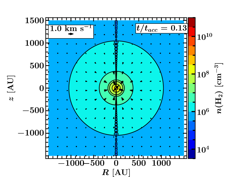
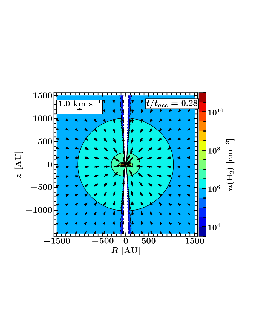
Figure 15: Gas density and velocity field for Model 3 at $t/t_{\rm acc}=0.13$ and 0.28 within 1500 AU. The density contours start from $\log(n/{\rm cm}^{-3})=5.5$ and increase by steps of 0.5 up to $\log(n/{\rm cm}^{-3})=9$. There are vertical and radial motions in the disk, which are not captured in this figure.

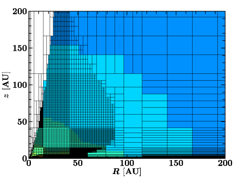
Figure 16: Example of the gridding used in the Stage 0 phase to resolve the small extent of the outflow cavity and to resolve the density and velocity gradient from the disk midplane to the envelope. The color contours are the same as in Fig. 15. The structure shown is for Model 1 at $t/t_{\rm acc}=0.13$.

Appendix B FIR and submm lines

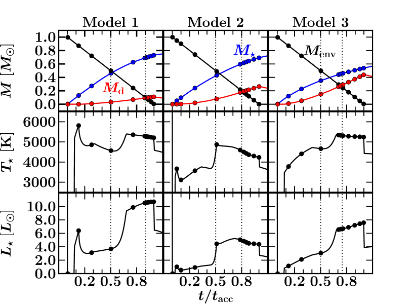
Figure 17: Evolution of the envelope, disk and stellar mass (top), effective stellar temperature (middle) and stellar luminosity (bottom) for the three different models as function of time (in units of $t_{\mathrm{acc}}$). The solid circles show the time steps (roughly around $t/t_{\rm acc}\sim 10^{-3},0.1,0.5,0.75,0.89,0.99$) used for rendering the molecular lines. The adopted time steps vary per model in order to cover properly the time when the model enters Stage 1 ($M_{\rm env}<M_{\star}$) and when the $M_{\rm d}=M_{\rm env}$ as indicated by the vertical dotted lines.

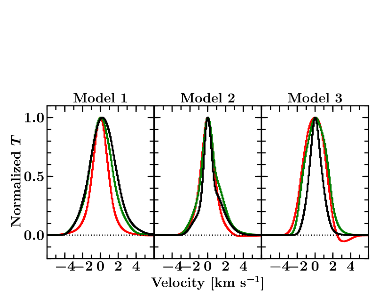
Figure 18: C¹⁸O $9-8$ line profiles convolved to a 9$\arcsec$ beam for the three models at $t/t_{\mathrm{acc}}=0.13$ (red), 0.50 (green) and 0.96 (black).

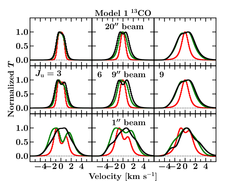
Figure 19: Normalized C¹⁸O and ¹³CO line profiles as functions of evolution for $J_{\mathrm{u}}=3$, 6 and 9 at $t/t_{\mathrm{acc}}=0.13$ (red), 0.50 (green) and 0.96 (black) for $i=5^{\circ}$ orientation for Model 1. The lines are convolved to beams of 20$\arcsec$ (top), 9$\arcsec$ (middle) and 1$\arcsec$ (bottom).

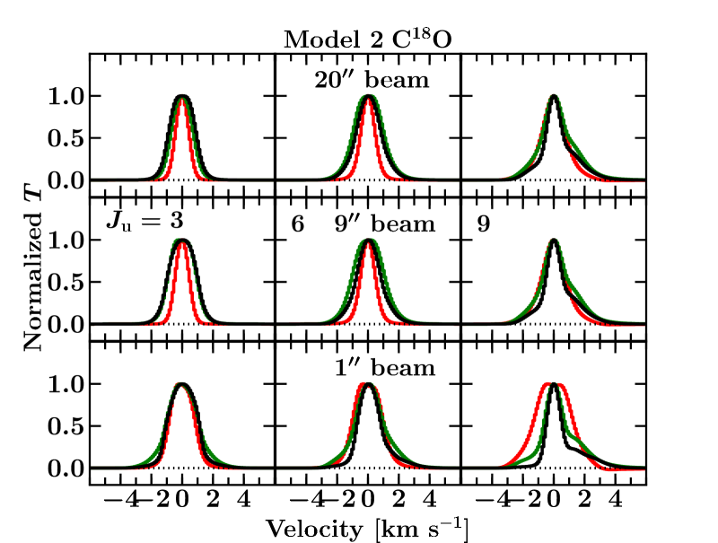
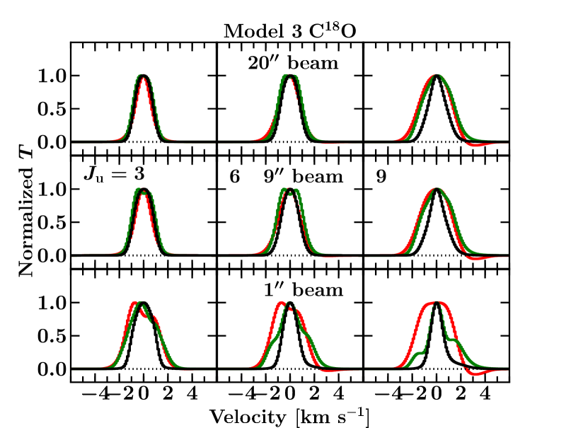
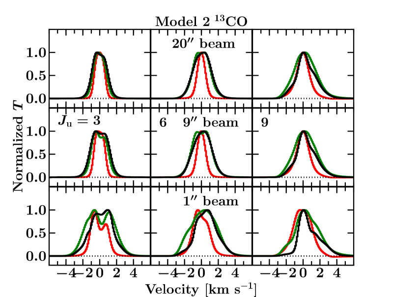
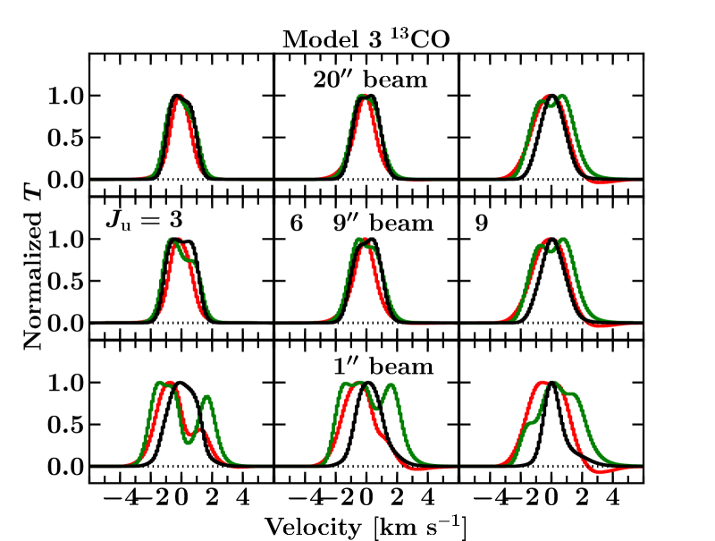
Figure 20: As Figure3, but for Models 2 and 3.

Figure 17 shows the mass evolution of the evolutionary models which indicates the times at which the models enter various evolutionary stages. Figure 18 presents the C¹⁸O 9–8 lines for the three different evolutionary models convolved to a 9$\arcsec$ beam. Most of the line is emitted from the inner envelope region. The line is generally broader in later stages due to a combination of thermal, turbulent width and velocity structure. However, the width of the line depends on whether the emitting region is infall or rotation dominated. Figures 19 and 20 shows the $J_{\rm u}=$3, 6 and 9 line profiles for the different models and how they change within different beams. The disk contribution to the observed lines within a 9$\arcsec$ beam is presented in Fig. 21 which is close to negligible for the low-$J$ lines.

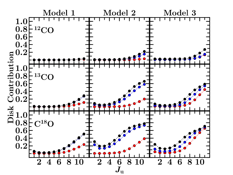
Figure 21: Disk contribution to total emission as a function of $J_{\mathrm{u}}$ within a 9${\arcsec}$ beam (1260 AU at 140 pc) for the three different models. The different colors correspond to different time steps: $t/t_{\mathrm{acc}}\sim 0.50$ (red), 0.75 (blue), 0.96 (black).

Appendix C NIR molecular lines

C.1 Inner disk

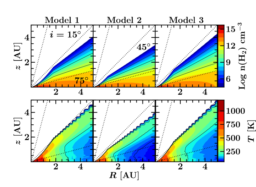
Figure 23: Density structure in the inner 10 AU (starting from n(H₂) = $10^{4.5}$ cm^-3) and temperature structure (starting from 60 K) of the three models. The three viewing angles are shown by dotted lines.

The formation of NIR continuum and the region where absorption happens depend on the physical structure in the inner few AU as will discussed extensively in the next section. Figure 23 shows the inner 5 AU structure of the three different models. In both Models 1 and 3, the $10^{4.5}$ cm^-3 density contour extends up to the line of sight of 45^∘ due to the presence of compact disk and massive disk, respectively. On the other hand, the density structure is flatter in Model 2. Thus, the NIR continuum emission is emitted through the high temperature region (mostly the red region in the temperature plot) and encounters more material along the line of sight to an observer in Models 1 and 3. Consequently, the emission from the region close to the midplane of the disk will not contribute to the NIR continuum. Figure 13 presents an example of the radial contribution to the column density along a line of sight from the star. At viewing angles $<45^{\circ}$, most of the warm material is located at 10–40 AU from the star along the line of sight while most of the cold material is located $>50$ AU. The inner disk and high density region ($<1$ AU) is only accessible through $i\geq 75^{\circ}$ in our models.

C.2 Radiative transfer effects

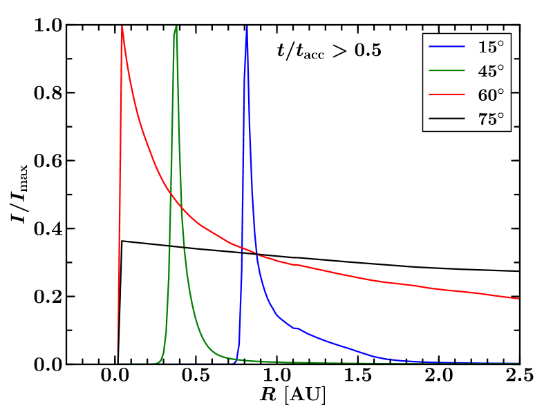
Figure 24: Normalized continuum flux without the stellar photosphere as function of distance from the center along one direction. The figure is constructed from a NIR image of Model 1 at $t/t_{\rm acc}=0.7$ as an example. The general trend is similar for $t/t_{\rm acc}>0.5$ independent of evolutionary models. The normalized continuum is similar for the various evolutionary models for $t/t_{\rm acc}>0.5$. The continuum is shown to arise in the inner few AU region and to fall off very quickly for $i<60^{\circ}$. However, significant contributions from larger radii are expected for relatively high inclination.

Section 4 discusses the RADLite results with respect to the predicted observables. In this section, we present the comparison between RADLite and a simple calculation using the integrated column density (column method, equation 3) to examine the radiative transfer effects in particular where the 4.7 $\mu$m continuum is formed and its affect on the simulated absorption lines.

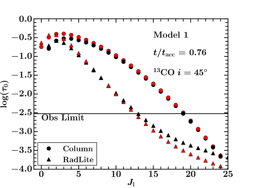
Figure 25: Comparison of the line center optical depth obtained from a simple integration of the column density along the line of sight (circles) and the radiative transfer calculation (triangles). The $P$ and $R$ branches are shown in black and red, respectively. The horizontal line indicates the current observation limit with CRIRES at $\tau\sim 3\times 10^{-3}$. The ¹³CO lines are shown for Model 1 at $t/t_{\rm acc}=0.76$ for $i=45^{\circ}$.

Figure 25 illustrates the difference in line center optical depth between the formal solution of the radiative transfer equation and the column density approach at $i=45^{\circ}$ (Eq. 3). This particular model and time was chosen as an example that clearly shows the difference. The difference in $\tau_{0}$ between the methods generally increases with $J_{\rm l}$ and are largest for $J_{\rm l}\sim 10$. Figure 24 shows the 4.7 $\mu$m continuum flux due to dust only (i.e., no stellar contribution) as function of radius at various viewing angles. The continuum is point-like for low inclinations but it is generally off-center for high inclinations. Thus, larger $\tau_{0}$ differences between the two methods are expected for larger inclinations since the absorption does not take place directly along the line of sight to the star. The implication is that the column method overestimates $\tau_{0}$ of the high-$J$ absorptions as this method takes the full line of sight through the warm material into account.

What are the implications for translating observed optical depths to column densities and excitation temperatures? The differences are largest for $J\geq 5$ lines which result in lower derived warm temperature and column densities in the full treatment. Consequently, the direct transformation from the observed optical depth to column density requires additional information on where the absorption arises, i.e., the NIR continuum image. One way is to construct the physical structure and assess the NIR continuum image. Observationally, a comparison between interferometric submm and NIR continuum should result in different continuum position if the NIR continuum arises from scattered light. Observationally driven constraint is likely more useful in practice since modelling of the NIR continuum requires a sophisticated inner disk and envelope physical structure. For systems with an off-centered NIR continuum, the derived column densities and temperature of the warm component are lower limits.

C.3 Non-LTE effects

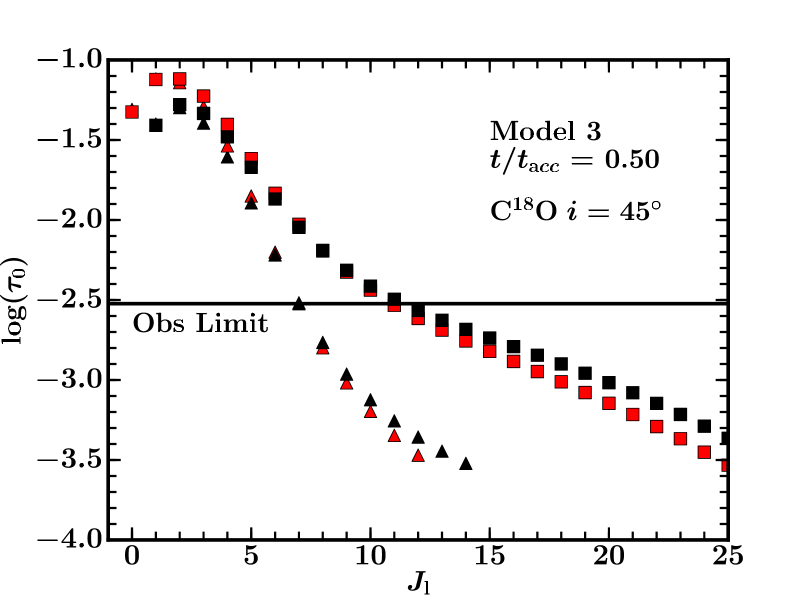
Figure 26: Comparison between LTE (squares) and non-LTE (triangles) line center optical depth obtained from RADLite for Model 3 at an inclination of 45^∘. The different colors correspond to the $P$ (black) and $R$ (red) branches.

The effects of non-LTE excitation in the vibrational ground state are studied by either using the level populations calculated with the full non-LTE escape probability method (§3) or assuming LTE populations. The LTE level population is calculated using the partition functions provided by the HITRAN database (Rothman et al. 2005).

Figure 26 compares LTE and non-LTE line center opacities of C¹⁸O for Model 3 at an inclination of 45^∘ (other isotopologs are shown in Figure 27). Model 3 was chosen as an example; in general, the non-LTE effects are most apparent for the higher levels independent of isotopologs and evolutionary models. This reflects the findings of §3: lower pure rotational levels are more easy to thermalize due to lower critical densities. The difference between LTE and non-LTE is independent of inclination while radiative transfer effects do. Thus, it is more important to treat the radiative transfer correctly in the NIR to derive observables.

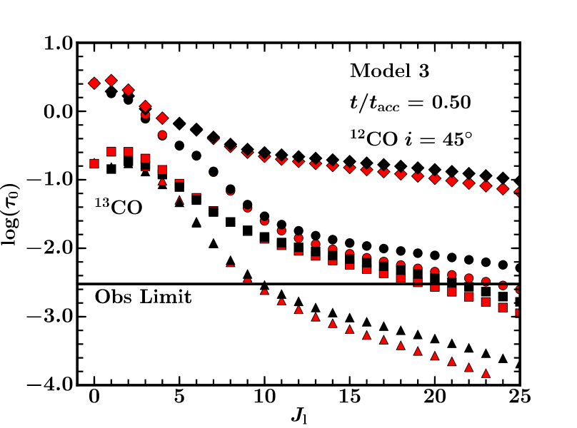
Figure 27: Similar to Fig. 26 for ¹²CO (diamonds and circles) and ¹³CO (squares and triangles).

References

- Aikawa et al. (2008) Aikawa, Y., Wakelam, V., Garrod, R. T., & Herbst, E. 2008, ApJ, 674, 984
- Baines et al. (2006) Baines, D., Oudmaijer, R. D., Porter, J. M., & Pozzo, M. 2006, MNRAS, 367, 737
- Belloche et al. (2002) Belloche, A., André, P., Despois, D., & Blinder, S. 2002, A&A, 393, 927
- Boogert et al. (2002) Boogert, A. C. A., Hogerheijde, M. R., & Blake, G. A. 2002, ApJ, 568, 761
- Brinch et al. (2007) Brinch, C., Crapsi, A., Jørgensen, J. K., Hogerheijde, M. R., & Hill, T. 2007, A & A, 475, 915
- Brinch et al. (2008) Brinch, C., Hogerheijde, M. R., & Richling, S. 2008, A & A, 489, 607
- Brinch et al. (2009) Brinch, C., Jørgensen, J. K., & Hogerheijde, M. R. 2009, A&A, 502, 199
- Brittain et al. (2005) Brittain, S. D., Rettig, T. W., Simon, T., & Kulesa, C. 2005, ApJ, 626, 283
- Brown et al. (2000) Brown, D. W., Chandler, C. J., Carlstrom, J. E., et al. 2000, MNRAS, 319, 154
- Bruderer et al. (2010) Bruderer, S., Benz, A. O., Stäuber, P., & Doty, S. D. 2010, ApJ, 720, 1432
- Bruderer et al. (2012) Bruderer, S., van Dishoeck, E. F., Doty, S. D., & Herczeg, G. J. 2012, A&A, 541, A91
- Cassen & Moosman (1981) Cassen, P. & Moosman, A. 1981, Icarus, 48, 353
- Chiang et al. (2008) Chiang, H.-F., Looney, L. W., K., T., Mundy, L. G., & Mouschovias, T. C. 2008, ApJ, 680, 474
- Crapsi et al. (2005) Crapsi, A., Devries, C. H., Huard, T. L., et al. 2005, A&A, 439, 1023
- Crapsi et al. (2008) Crapsi, A., van Dishoeck, E., Hogerheijde, M. R., Pontoppidan, K., & Dullemond, C. 2008, A&A, 486, 245
- Dapp & Basu (2010) Dapp, W. B. & Basu, S. 2010, A&A, 521, L56
- Dapp et al. (2012) Dapp, W. B., Basu, S., & Kunz, M. W. 2012, A&A, 541, A35
- de Graauw et al. (2010) de Graauw, T., Helmich, F. P., Phillips, T. G., et al. 2010, A&A, 518, L6
- Doty et al. (2004) Doty, S. D., Schöier, F. L., & van Dishoeck, E. F. 2004, A&A, 418, 1021
- Doty et al. (2002) Doty, S. D., van Dishoeck, E. F., van der Tak, F. F. S., & Boonman, A. M. S. 2002, A&A, 389, 446
- Dunham et al. (2010) Dunham, M. M., Evans, N. J., Terebey, S., Dullemond, C. P., & Young, C. H. 2010, ApJ, 710, 470
- Enoch et al. (2009) Enoch, M. L., Corder, S., Dunham, M. M., & Duchêne, G. 2009, ApJ, 707, 103
- Evans (1999) Evans, II, N. J. 1999, ARA&A, 37, 311
- Evans et al. (2005) Evans, II, N. J., Lee, J.-E., Rawlings, J. M. C., & Choi, M. 2005, ApJ, 626, 919
- Goicoechea et al. (2012) Goicoechea, J. R., Cernicharo, J., Karska, A., et al. 2012, A&A, 548, A77
- Griffin et al. (2010) Griffin, M. J., Abergel, A., Abreu, A., et al. 2010, A&A, 518, L3
- Harsono et al. (2011) Harsono, D., Alexander, R. D., & Levin, Y. 2011, MNRAS, 413, 423
- Hayashi et al. (1993) Hayashi, M., Ohashi, N., & Miyama, S. M. 1993, ApJ, 418, L71
- Herczeg et al. (2011) Herczeg, G. J., Brown, J. M., van Dishoeck, E. F., & Pontoppidan, K. M. 2011, A&A, 533, 112
- Herczeg et al. (2012) Herczeg, G. J., Karska, A., Bruderer, S., et al. 2012, A&A, 540, A84
- Hogerheijde (2001) Hogerheijde, M. R. 2001, ApJ, 553, 618
- Hogerheijde & Sandell (2000) Hogerheijde, M. R. & Sandell, G. 2000, ApJ, 534, 880
- Hogerheijde et al. (1998) Hogerheijde, M. R., van Dishoeck, E. F., Blake, G. A., & van Langevelde, H. J. 1998, ApJ, 502, 315
- Joos et al. (2012) Joos, M., Hennebelle, P., & Ciardi, A. 2012, A&A, 543, A128
- Jørgensen et al. (2009) Jørgensen, J. K., Bourke, T. L., Myers, P. C., et al. 2009, A&A, 507, 861
- Jørgensen et al. (2005) Jørgensen, J. K., Bourke, T. L., Myers, P. C., et al. 2005, ApJ, 632, 973
- Jørgensen et al. (2002) Jørgensen, J. K., Schöier, F. L., & van Dishoeck, E. F. 2002, A&A, 389, 908
- Keene & Masson (1990) Keene, J. & Masson, C. R. 1990, ApJ, 355, 635
- Kratter et al. (2010) Kratter, K. M., Matzner, C. D., Krumholz, M. R., & Klein, R. I. 2010, ApJ, 708, 1585
- Kristensen et al. (2012) Kristensen, L. E., van Dishoeck, E. F., Bergin, E. A., et al. 2012, A&A, 542, 8
- Lee et al. (2004) Lee, J.-E., Bergin, E. A., & Evans, N. J. 2004, ApJ, 617, 360
- Lee et al. (2005) Lee, J.-E., Evans, N. J., & Bergin, E. A. 2005, ApJ, 631, 351
- Li et al. (2011) Li, Z.-Y., Krasnopolsky, R., & Shang, H. 2011, ApJ, 738, 180
- Lommen et al. (2008) Lommen, D., Jørgensen, J. K., van Dishoeck, E. F., & Crapsi, A. 2008, A&A, 481, 141
- Lynden-Bell & Pringle (1974) Lynden-Bell, D. & Pringle, J. E. 1974, MNRAS, 168, 603
- Manoj et al. (2013) Manoj, P., Watson, D. M., Neufeld, D. A., et al. 2013, ApJ, 763, 83
- Maury et al. (2010) Maury, A. J., André, P., Hennebelle, P., et al. 2010, A&A, 512, 40
- Mitchell et al. (1990) Mitchell, G. F., Maillard, J.-P., Allen, M., Beer, R., & Belcourt, K. 1990, ApJ, 363, 554
- Ohashi et al. (1997) Ohashi, N., Hayashi, M., Ho, P. T. P., et al. 1997, ApJ, 488, 317
- Poglitsch et al. (2010) Poglitsch, A., Waelkens, C., Geis, N., et al. 2010, A&A, 518, L2
- Pontoppidan et al. (2008) Pontoppidan, K. M., Blake, G. A., van Dishoeck, E. F., et al. 2008, ApJ, 684, 1323
- Pontoppidan et al. (2009) Pontoppidan, K. M., Meijerink, R., Dullemond, C. P., & Blake, G. a. 2009, ApJ, 704, 1482
- Robitaille et al. (2007) Robitaille, T. P., Whitney, B. A., Indebetouw, R., & Wood, K. 2007, ApJ, 169, 328
- Robitaille et al. (2006) Robitaille, T. P., Whitney, B. A., Indebetouw, R., Wood, K., & Denzmore, P. 2006, ApJS, 167, 256
- Rothman et al. (2005) Rothman, L. S., Jacquemart, D., Barbe, A., et al. 2005, J. Quant. Spectrosc. Radiat. Transfer, 96, 139
- Saito et al. (1996) Saito, M., Kawabe, R., Kitamura, Y., & Sunada, K. 1996, ApJ, 473, 464
- San Jose-Garcia et al. (2013) San Jose-Garcia, I., Mottram, J. C., Kristensen, L. E., et al. 2013, A&A, in press
- Sargent & Beckwith (1987) Sargent, A. I. & Beckwith, S. 1987, ApJ, 323, 294
- Sault et al. (1995) Sault, R. J., Teuben, P. J., & Wright, M. C. 1995, Astronomical Data Analysis Software and Systems IV, 77, 433
- Schöier et al. (2005) Schöier, F. L., van der Tak, F. F. S., van Dishoeck, E. F., & Black, J. H. 2005, A& A, 432, 369
- Shakura & Sunyaev (1973) Shakura, N. I. & Sunyaev, R. A. 1973, A&A, 24, 337
- Shu (1977) Shu, F. H. 1977, ApJ, 214, 488
- Smith et al. (2010) Smith, R. L., Pontoppidan, K. M., Young, E. D., & Morris, M. R. 2010, in Lunar and Planetary Inst. Technical Report, Vol. 41, Lunar and Planetary Institute Science Conference Abstracts, 2254
- Smith et al. (2009) Smith, R. L., Pontoppidan, K. M., Young, E. D., Morris, M. R., & van Dishoeck, E. F. 2009, ApJ, 701, 163
- Spaans et al. (1995) Spaans, M., Hogerheijde, M. R., Mundy, L. G., & van Dishoeck, E. F. 1995, APJL, 455, 167
- Spitzer (1989) Spitzer, Jr., L. 1989, ARA&A, 27, 1
- Takahashi et al. (1983) Takahashi, T., Silk, T., & Holenbach, D. J. 1983, ApJ, 275, 145
- Takakuwa et al. (2012) Takakuwa, S., Saito, M., Lim, J., et al. 2012, ApJ, 754, 52
- Takami et al. (2001) Takami, M., Bailey, J., Gledhill, T. M., Chrysostomou, A., & Hough, J. H. 2001, MNRAS, 323, 177
- Terebey et al. (1984) Terebey, S., Shu, F. H., & Cassen, P. 1984, ApJ, 286, 529
- Tobin et al. (2011) Tobin, J. J., Hartmann, L., Chiang, H.-F., et al. 2011, ApJ, 740, 42
- Tobin et al. (2012) Tobin, J. J., Hartmann, L., Chiang, H.-F., et al. 2012, Nature, 492, 83
- van Kempen et al. (2010) van Kempen, T. A., Kristensen, L. E., Herczeg, G. J., et al. 2010, A&A, 518, A121
- van Kempen et al. (2009a) van Kempen, T. A., van Dishoeck, E. F., Güsten, R., et al. 2009a, A&A, 501, 633
- van Kempen et al. (2009b) van Kempen, T. A., van Dishoeck, E. F., Güsten, R., et al. 2009b, A&A, 507, 1425
- van Kempen et al. (2009c) van Kempen, T. A., van Dishoeck, E. F., Salter, D. M., et al. 2009c, A&A, 498, 167
- van Weeren et al. (2009) van Weeren, R. J., Brinch, C., & Hogerheijde, M. R. 2009, A&A, 497, 773
- Visser & Bergin (2012) Visser, R. & Bergin, E. A. 2012, ApJ, 754, L18
- Visser et al. (2011) Visser, R., Doty, S. D., & van Dishoeck, E. F. 2011, A&A, 534, A132
- Visser & Dullemond (2010) Visser, R. & Dullemond, C. P. 2010, A&A, 519, A28
- Visser et al. (2012) Visser, R., Kristensen, L. E., Bruderer, S., et al. 2012, A&A, 537, A55
- Visser et al. (2009) Visser, R., van Dishoeck, E. . F., Doty, S., & Dullemond, C. P. 2009, A&A, 495, 881
- Whitney et al. (2003) Whitney, B. A., Wood, K., Bjorkman, J. E., & Wolff, M. J. 2003, ApJ, 598, 1079
- Wilson & Rood (1994) Wilson, T. L. & Rood, R. 1994, ARA&A, 32, 191
- Yang et al. (2010) Yang, B., Stancil, P. C., Balakrishnan, N., & Forrey, R. C. 2010, ApJ, 718, 1062
- Yıldız et al. (2013) Yıldız, U., Kristensen, L., van Dishoeck, E., et al. 2013, A&A, subm.
- Yıldız et al. (2012) Yıldız, U. A., Kristensen, L. E., van Dishoeck, E. F., et al. 2012, A&A, 542, A86
- Yıldız et al. (2010) Yıldız, U. A., van Dishoeck, E. F., Kristensen, L. E., et al. 2010, A&A, 521, L40
- Young & Evans (2005) Young, C. H. & Evans, N. J. 2005, ApJ, 627, 293
- Young et al. (2004) Young, C. H., Jørgensen, J. K., Shirley, Y. L., et al. 2004, ApJS, 154, 396
- Zhou et al. (1993) Zhou, S., Evans, N. J., Kömpe, C., & Walmsley, C. M. 1993, ApJ, 404, 232