Single-Spin Asymmetries in Semi-inclusive Deep Inelastic Scattering and Drell-Yan Processes

Abstract

We examine in detail the diagrammatic mechanisms which provide the change of sign between the single transverse spin asymmetries measured in semi-inclusive deep inelastic scattering (SIDIS) and in the Drell-Yan process (DY). This asymmetry is known to arise due to the transverse spin dependence of the target proton combined with a $T$-odd complex phase. Using the discrete symmetry properties of transverse spinors, we show that the required complex phase originates in the denominators of rescattering diagrams and their respective cuts. For simplicity, we work in a model where the proton consists of a valence quark and a scalar diquark. We then show that the phases generated in SIDIS and in DY originate from distinctly different cuts in the amplitudes, which at first appears to obscure the relationship between the single-spin asymmetries in the two processes. Nevertheless, further analysis demonstrates that the contributions of these cuts are identical in the leading-twist Bjorken kinematics considered, resulting in the standard sign-flip relation between the Sivers functions in SIDIS and DY. Physically, this fundamental, but yet untested, prediction occurs because the Sivers effect in the Drell-Yan reaction is modified by the initial-state “lensing” interactions of the annihilating antiquark, in contrast to the final-state lensing which produces the Sivers effect in deep inelastic scattering.

PACS numbers: 12.38.Bx, 13.88.+e

1 Introduction

1.1 Factorization and Final State Interactions

The factorization picture of leading twist-perturbative QCD has played a guiding role in virtually all aspects of hadron physics phenomenology. In the case of inclusive reactions such as hadroproduction at large transverse momentum $p+p\to H+X$ [1, 2], the parton model for perturbative quantum chromodynamics (pQCD) predicts that the cross section at leading order in the transverse momentum $p_{T}$ can be computed by convoluting the perturbatively calculable hard subprocess quark and gluon cross section with the process-independent structure functions of the colliding hadrons and the final-state quark or gluon fragmentation functions. The resulting leading-twist cross section $E_{H}{d\sigma/d^{3}p_{H}}(pp\to HX)$ scales as $1/p^{4}_{T},$ modulo the DGLAP scaling violations derived from the logarithmic evolution of the structure functions and fragmentation distributions, as well as the running of the QCD coupling appearing in the hard-scattering subprocess matrix element.

The effects of final-state interactions of the scattered quark in deep inelastic scattering are characterized by a Wilson line. Such effects have traditionally been assumed to either give an inconsequential phase factor or power-law suppressed corrections in hard pQCD reactions. However, this expectation is only true for sufficiently inclusive cross sections. For example, consider semi-inclusive deep inelastic lepton scattering (SIDIS) on a transversely polarized target $\ell+p^{\uparrow}\to H+\ell^{\prime}+X$. (For a review see [3].) In this case the final-state gluonic interactions of the scattered quark lead to a pseudo-$T$-odd non-zero spin correlation of the lepton-quark scattering plane with the polarization of the target proton [4] which is not power-law suppressed with increasing virtuality of the photon $Q^{2}$; i.e., it Bjorken-scales. This asymmetry is made experimentally explicit by studying the triple product of vectors $\vec{S}_{P}\cdot(\vec{q}\times{\vec{p}}_{H})$, where ${\vec{p}}_{H}$ is the momentum of the hadron fragmented from the struck quark jet. Similar correlations can be found from target spin asymmetries, due to multi-photon exchanges [5].

A crucial fact is that the leading-twist “Sivers effect” [6, 7] is non-universal in the sense that pQCD predicts an opposite-sign correlation in Drell-Yan reactions relative to semi-inclusive deep inelastic scattering [8, 9]. This fundamental, but yet untested, prediction occurs because the Sivers effect in the Drell-Yan reaction is modified by the initial-state “lensing” interactions of the annihilating antiquark, in contrast to the final-state lensing which produces the Sivers effect in deep inelastic scattering.

The calculation of the Sivers single-spin asymmetry in deep inelastic lepton scattering in QCD is illustrated schematically in Fig. 1. Although the Coulomb phase for a given partial wave is infinite, the interference of Coulomb phases arising from different partial waves leads to observable effects. The analysis requires two different orbital angular momentum components: $S$-wave with the quark-spin parallel to the proton spin and $P$-wave for the quark with anti-parallel spin; the difference between the final-state “Coulomb” phases leads to a $\vec{S}\cdot(\vec{q}\times\vec{p})$ correlation of the proton’s spin with the virtual photon-to-quark production plane [4]. Thus, as it is clear from its QED analog, the final-state gluonic interactions of the scattered quark lead to a pseudo–$T$-odd non-zero spin correlation of the lepton-quark scattering plane with the polarization of the target proton [4]. The effect is pseudo-T odd due to the imaginary phase generated by the cut of the near-on-shell intermediate state.

The $S$- and $P$-wave proton wavefunctions also appear in the calculation of the Pauli form factor quark-by-quark. Thus one can correlate the Sivers asymmetry for each struck quark with the anomalous magnetic moment of the proton carried by that quark [10], leading to the prediction that the Sivers effect is larger for positive pions as seen by the HERMES experiment at DESY [11], the COMPASS experiment [12, 13, 14, 15] at CERN, and CLAS at Jefferson Laboratory [16, 17].

The final-state interactions of the produced quark with its comoving spectators in SIDIS also produces a final-state $T$-odd polarization correlation – the “Collins effect”, in which the Collins fragmentation function, instead of the Sivers distribution function, generates the spin asymmetry [18, 19]. This can be measured without beam polarization by measuring the correlation of the polarization of a hadron such as the $\Lambda$ baryon with the quark-jet production plane [20, 21, 22, 23]. Analogous spin effects occur in reactions in QED due to the rescattering via final-state Coulomb interactions.

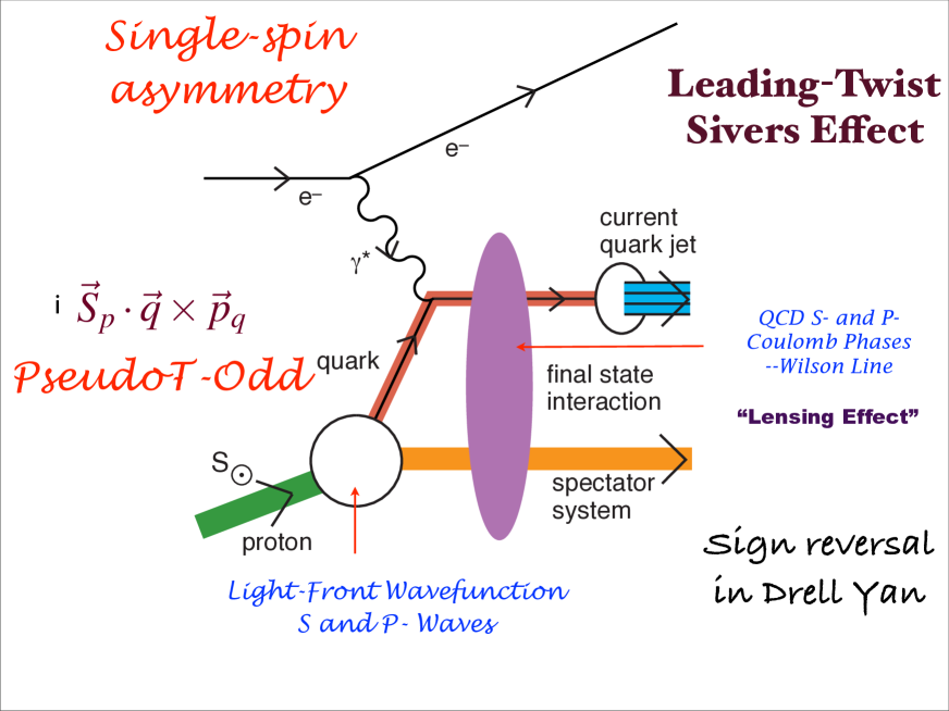
Figure 1: Origin of the Sivers single-spin asymmetry in semi-inclusive deep inelastic lepton scattering.

In principle, the physics of the “lensing dynamics” or Wilson-line physics [24, 25] underlying the Sivers effect involves nonperturbative quark-quark interactions at small momentum transfer, not the hard scale $Q^{2}$ of the virtuality of the photon. These considerations have thus led to a reappraisal of the range of validity of the standard factorization ansatz. As noted by Collins and Qiu [26], the traditional factorization formalism of perturbative QCD fails in detail for many hard inclusive reactions because of initial- and final-state lensing interactions. For example, if both the quark and antiquark in the Drell-Yan subprocess $q+\bar{q}\to\mu^{+}+\mu^{-}$ interact with the spectators of the other hadron, then one predicts a $\cos 2\phi\,\sin^{2}\theta$ planar correlation in unpolarized Drell-Yan reactions [27]. (Here $\phi$ is the angle between the muon plane and the plane of the incident hadrons in the lepton pair center of mass frame, while $\theta$ is the angle between the momentum of one of the muons and the line of flight of partons in the same frame [27, 28].) This “double Boer-Mulders effect” [19] can account for the anomalously large $\cos 2\phi$ correlation and the corresponding violation [27, 29] of the Lam-Tung relation [30, 31] for Drell-Yan processes observed by the NA10 collaboration [28], and the azimuthal angle dependence of di-jet production in unpolarized hadron scattering [32]. Such effects again point to the importance of the corrections from initial and final-state interactions of the hard-scattering constituents, which are not included in the standard pQCD factorization formalism.

The final-state interactions of the struck quark with the target spectators [33] also lead to diffractive events in deep inelastic scattering (DIS) at leading twist, such as $\ell+p\to\ell^{\prime}+p^{\prime}+X$, where the proton remains intact and isolated in rapidity; in fact, approximately 10 % of the deep inelastic lepton-proton scattering events observed at HERA are diffractive [34, 35]. The presence of a rapidity gap between the target and diffractive system requires that the target remnant emerges in a color-singlet state; this is made possible in any gauge by the soft rescattering incorporated in the Wilson line or by augmented light-front wavefunctions.

1.2 The Sign of the Sivers Effect

As we have emphasized in the above, the sign reversal predicted by QCD between the Sivers functions [6, 7, 9] in semi-inclusive deep inelastic scattering (SIDIS) and in the Drell-Yan process (DY) [8, 9] is in contrast to the standard expectations of collinear pQCD/parton model factorization. This reversal results in different signs predicted for the single transverse spin asymmetry (SSA) in SIDIS on a transversely polarized proton versus that in the DY process involving a transversely polarized hadron. The sign difference of the Sivers functions is a consequence of their being pseudo $T$-odd, with the SIDIS Sivers function related to the DY Sivers function by a time-reversal transformation [8, 36, 37]. The essential physics of the sign change is illustrated for QED in Fig. 2. The final-state interaction in SIDIS is attractive whereas the initial-state interaction is repulsive in DY. However, the detailed analysis involves many subtle aspects due to intermediate Glauber-type cuts related to unitarity. These considerations are worked out in detail in this article.

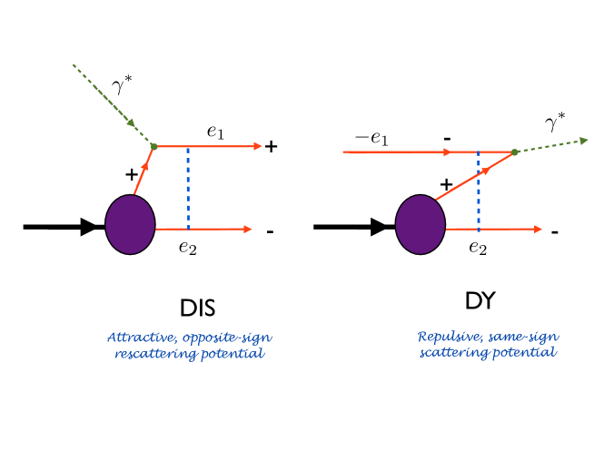
Figure 2: The underlying physics of the sign change of the lensing interactions in SIDIS and DY reactions for QED. Dashed lines denote the photon propagators. The final-state interaction in SIDIS is attractive whereas the initial state interaction is repulsive in DY.

In general, the generation of a SSA requires two ingredients: (i) the dependence of the cross section on the transverse polarization, and (ii) a relative complex phase between the amplitudes corresponding to different orbital angular momenta [38, 39, 40]. In the original argument given by Collins [8] the sign flip between SSA in SIDIS and DY arises due to a reversal of the direction of the Wilson line in the definition of the Sivers function under the application of $T$-reversal. It is interesting and important to clarify the relation between this time-reversal argument and the diagrammatic conditions (i) and (ii) stated above. While it is well-known that the propagation of a high energy quark or gluon can be approximated by a Wilson line along the corresponding light cone direction, the connection between the Wilson lines and Feynman diagrams can be non-trivial [41], especially in the SSA case, where we are interested in the imaginary part of the scattering amplitude due to the condition (ii) above. Establishing a clear connection in the Feynman diagram language between the spin asymmetries in SIDIS and DY will greatly aid future (model) diagrammatic calculations for the processes.

Although the time-reversal symmetry argument allows one to confidently predict the sign flip between the Sivers functions in the two processes, a detailed diagrammatic model calculation demonstrating the origin of this sign reversal appears to be lacking in the literature. A model calculation for the SSA in SIDIS was first constructed in [9] by some of the authors; however, an analogous calculation for DY outlined in [4] assumed that the relative phase arises in DY due to putting the same propagators as in SIDIS on mass shell. As we will show below, one can think of the relative phase from the condition (ii) as a cut through an amplitude (or a complex conjugate amplitude), in addition to the standard final-state cut one obtains when the scattering amplitude is squared. In terms of the cuts, the calculation of [4] assumed that the cut generating SSA in SIDIS was equivalent to the cut in DY. While this assumption allows one to obtain the correct answer with the sign flip in the Sivers function between SIDIS and DY, as we shall discuss below, it is not easy to justify. In fact, the explicit calculation of the SSA in the SIDIS and DY processes given in this paper demonstrates that the cuts are, in fact, different, as illustrated in Figures 4 and 6. In Feynman diagram language this means that different propagators are put on the mass shell in order to extract the asymmetry in the two processes. In light-front perturbation theory (LFPTH) [42, 43] language this corresponds to putting different intermediate states (that is, intermediate states involving different particles) on the $P^{-}$ LF energy shell.

One may then wonder how the simple sign-flip relation between the Sivers functions in SIDIS and DY would arise from Feynman diagrams with different cuts (or LFPTH diagrams with different intermediate states put on energy shell). While further clarification of the diagrammatic origin of the sign flip is left for future work, we shall show here by performing an explicit calculation that in the limit of high energy $s$ and high photon virtuality $Q^{2}$, the simple sign-flip relationship is preserved for SIDIS and DY Sivers functions, despite the different cuts in the diagrams in the two cases. We thus are able to construct a diagrammatic description of the sign reversal.

The paper is structured as follows. In Section 2 we show how the transverse polarization dependence always comes into the amplitude squared with the imaginary factor of $i$. Since the cross section contribution has to be real, this implies that, for the spin asymmetry to be non-zero, another factor of $i$ has to be generated elsewhere in the amplitude squared. We thus demonstrate the need for a phase difference between the amplitude and the complex conjugate amplitude contributing to the SSA [39, 40]. Our analysis provides an explicit verification of the analytical properties of the complete amplitudes.

In Section 3 we perform a model calculation of the spin asymmetry in the SIDIS and DY cases using a Feynman diagram approach. We employ a model in which the proton is made out of a valence quark and a scalar color-charged diquark: this model was used previously in [4, 9]. Instead of calculating the Sivers functions directly, we consider the $\gamma^{*}+p^{\uparrow}\to q+X$ process in place of the SIDIS Sivers function, and the ${\bar{q}}+p^{\uparrow}\to\gamma^{*}+X$ process in place of the DY Sivers function. It can be shown that the relation between these processes and the corresponding Sivers functions is the same in both cases (see [27] for an example of how to establish the connection): hence, the sign reversal of the SSAs in the $\gamma^{*}+p^{\uparrow}\to q+X$ and ${\bar{q}}+p^{\uparrow}\to\gamma^{*}+X$ processes is equivalent to the sign flips in the corresponding Sivers functions.

Performing an explicit calculation in Section 3 we demonstrate that, in the framework of the model considered, the SSAs in SIDIS and DY arise from different cuts, as shown in Figs. 4 and 6. Nevertheless, the resulting spin asymmetries only differ by a minus sign, in agreement with the general arguments based on time-reversal anti-symmetry [8, 36]. We demonstrate how the same conclusion can be achieved in a LFPTH calculation in Section 4: while different LF energy denominators are put on energy shell in SIDIS and DY, the resulting SSA in DY is simply a negative of that in the SIDIS case. Section 5 summarizes our main results.

2 Coupling of Transverse Spinors to the Complex Phase

The discrete symmetries of the Dirac equation, $\mathrm{C,P}$ and $\mathrm{T}$ provide strong constraints on the form of the spinors and their matrix elements. In particular, the $\mathrm{PT}$ properties of transverse spinors bring in a unique coupling of the transverse spin dependence of a matrix element to its real and imaginary parts. This gives rise to the conclusion that the single transverse spin asymmetry requires the presence of a complex phase aside from the spinor matrix elements themselves.

Below, we explicitly construct the transverse spinors and the identities they satisfy corresponding to $\mathrm{C/P/T}$ transformations. We demonstrate that, as a consequence, when two spinor matrix elements are multiplied together (as in the numerator of a scattering amplitude squared), the part which depends on the transverse spin is pure imaginary.

We then define the asymmetry observable $A_{N}$ and use the knowledge of the $\mathrm{C/P/T}$ constraints to identify which types of diagrams can contribute to the asymmetry. We find that only interference terms can contribute to $A_{N}$, and furthermore only the imaginary part of the interference term (aside from the spinor products) contributes. We derive an expression for the spin-difference part of the amplitude squared in terms of the imaginary part of the rest of the interference term.

2.1 Spinor Conventions and $\mathrm{C/P/T}$ Identities

In this calculation we will work with the spinors defined in Ref. [42]. These spinors correspond to the spin projection along the $\pm z$ axis of a particle with mass $m$ and are expressed in light-cone coordinates $p^{\pm}\equiv p^{(0)}\pm p^{(3)}$. For definiteness, working in the standard (Dirac) representation of the Clifford algebra, this spinor basis is:

$$U_{+z}(p) =\frac{1}{\sqrt{2p^{+}}}\left[\begin{array}[]{c}p^{+}+m\\ p^{(1)}+ip^{(2)}\\ p^{+}-m\\ p^{(1)}+ip^{(2)}\end{array}\right]\hskip 28.45274ptU_{-z}(p) =\frac{1}{\sqrt{2p^{+}}}\left[\begin{array}[]{c}-p^{(1)}+ip^{(2)}\\ p^{+}+m\\ p^{(1)}-ip^{(2)}\\ -p^{+}+m\end{array}\right]$$ (9)

$$V_{+z}(p) =\frac{1}{\sqrt{2p^{+}}}\left[\begin{array}[]{c}-p^{(1)}+ip^{(2)}\\ p^{+}-m\\ p^{(1)}-ip^{(2)}\\ -p^{+}-m\end{array}\right]\hskip 28.45274ptV_{-z}(p) =\frac{1}{\sqrt{2p^{+}}}\left[\begin{array}[]{c}p^{+}-m\\ p^{(1)}+ip^{(2)}\\ p^{+}+m\\ p^{(1)}+ip^{(2)}\end{array}\right].$$ (18)

Like any spinor basis for solutions of the Dirac equation, these spinors satisfy identities that embody the discrete $\mathrm{C}$, $\mathrm{P}$, and $\mathrm{T}$ symmetries of the theory. As can be explicitly verified from (9), these spinors obey the identities

$$\mathrm{C:}\hskip 28.45274pt -i\gamma^{2}V_{\pm z}^{*}(p)=U_{\pm z}(p)$$ (19)

$$\mathrm{PT:}\hskip 28.45274pt \gamma^{1}\gamma^{3}\gamma^{0}U_{\pm z}^{*}(p)=\mp U_{\mp z}(p)$$

$$\gamma^{1}\gamma^{3}\gamma^{0}V_{\pm z}^{*}(p)=\pm V_{\mp z}(p)$$

$$\mathrm{CPT:}\hskip 28.45274pt U_{\pm z}(p)=\pm\gamma^{5}V_{\mp z}(p),$$

where the final $\mathrm{CPT}$ identity combines the other two in a compact form.

For our purposes, we are interested in transverse spin states. If we choose a frame in which the incoming polarized particle moves along the $+z$ axis such that $\vec{p}_{\bot}=\vec{0}_{\bot}$, then the spinors (9) become eigenstates of the helicity operator. We can form transverse spinors as done in [44] by taking linear combinations of (9) to obtain the projection along, say, the $x$ axis:

$$U_{\chi} =\frac{1}{\sqrt{2}}(U_{+z}+\chi U_{-z})$$ (20)

$$V_{\chi} =\frac{1}{\sqrt{2}}(V_{+z}-\chi V_{-z}),$$

where $\chi=\pm 1$ is the spin eigenvalue along the $x$ axis. Again, for a $\vec{p}_{\bot}=\vec{0}_{\bot}$ incoming particle, these spinors reflect a spin projection transverse to the beam axis; they are simultaneous eigenstates of the Dirac operator as well as the Pauli-Lubanski vector $W_{1}$, where $W_{\mu}\equiv-\frac{1}{2}\epsilon_{\mu\nu\rho\sigma}S^{\nu\rho}p^{\sigma}$.

Using (19) in (20) gives the somewhat different $\mathrm{C/P/T}$ identities satisfied by the transverse spinors:

$$\mathrm{C}:\hskip 28.45274pt -i\gamma^{2}V_{\chi}^{*}(p)=U_{-\chi}(p)$$ (21)

$$\mathrm{CPT}:\hskip 28.45274pt U_{\chi}(p)=-\chi\gamma^{5}V_{\chi}(p).$$

Employing and generalizing (21) allows us to write a complete set of identities for any transverse spinor matrix element:

$$\mathrm{C:}\hskip 28.45274pt\overline{V}_{\chi^{\prime}}(k)\gamma^{\mu_{1}}\cdots\gamma^{\mu_{n}}V_{\chi}(p) = \left[\overline{V}_{\chi}(p)\gamma^{\mu_{n}}\cdots\gamma^{\mu_{1}}V_{\chi^{\prime}}(k)\right]^{*}$$

$$= (-1)^{n-1}\overline{U}_{-\chi}(p)\gamma^{\mu_{n}}\cdots\gamma^{\mu_{1}}U_{-\chi^{\prime}}(k)$$

$$= (-1)^{n-1}\left[\overline{U}_{-\chi^{\prime}}(k)\gamma^{\mu_{1}}\cdots\gamma^{\mu_{n}}U_{-\chi}(p)\right]^{*}$$

$$\mathrm{C:}\hskip 28.45274pt\overline{U}_{\chi^{\prime}}(k)\gamma^{\mu_{1}}\cdots\gamma^{\mu_{n}}V_{\chi}(p) = \left[\overline{V}_{\chi}(p)\gamma^{\mu_{n}}\cdots\gamma^{\mu_{1}}U_{\chi^{\prime}}(k)\right]^{*}$$

$$= (-1)^{n-1}\overline{U}_{-\chi}(p)\gamma^{\mu_{n}}\cdots\gamma^{\mu_{1}}V_{-\chi^{\prime}}(k)$$

$$= (-1)^{n-1}\left[\overline{V}_{-\chi^{\prime}}(k)\gamma^{\mu_{1}}\cdots\gamma^{\mu_{n}}U_{-\chi}(p)\right]^{*}$$

$$\mathrm{CPT:}\hskip 28.45274pt\overline{V}_{\chi^{\prime}}(k)\gamma^{\mu_{1}}\cdots\gamma^{\mu_{n}}U_{\chi}(p) = \chi\chi^{\prime}\left[\overline{V}_{-\chi^{\prime}}(k)\gamma^{\mu_{1}}\cdots\gamma^{\mu_{n}}U_{-\chi}(p)\right]^{*}$$ (24)

$$\overline{U}_{\chi^{\prime}}(k)\gamma^{\mu_{1}}\cdots\gamma^{\mu_{n}}U_{\chi}(p) = \chi\chi^{\prime}\left[\overline{U}_{-\chi^{\prime}}(k)\gamma^{\mu_{1}}\cdots\gamma^{\mu_{n}}U_{-\chi}(p)\right]^{*}.$$

These identities allow us to explicitly determine rigid constraints on the form of any transverse spinor product. In particular, consider the parameterizations of both classes of spinor products:

$$\overline{V}_{\chi^{\prime}}(k)\gamma^{\mu_{1}}\cdots\gamma^{\mu_{n}}U_{\chi}(p)\, \equiv \,\delta_{\chi\chi^{\prime}}[a(k,p)+\chi a^{\prime}(k,p)]+\delta_{\chi,-\chi^{\prime}}[b(k,p)+\chi b^{\prime}(k,p)]$$ (25)

$$\overline{U}_{\chi^{\prime}}(k)\gamma^{\mu_{1}}\cdots\gamma^{\mu_{n}}U_{\chi}(p)\, \equiv \,\delta_{\chi\chi^{\prime}}[c(k,p)+\chi c^{\prime}(k,p)]+\delta_{\chi,-\chi^{\prime}}[d(k,p)+\chi d^{\prime}(k,p)];$$

applying (24), one readily concludes that $\mathrm{C/P/T}$ constraints imply that:

• $a$, $b^{\prime}$, $c$, and $d^{\prime}$ are real-valued.

• $a^{\prime}$, $b$, $c^{\prime}$, and $d$ are pure imaginary.

Furthermore, this implies that if we multiply any two of these spinor matrix elements and sum over one of the spins ($\chi^{\prime}$), e.g.,

$$\sum_{\chi^{\prime}} \,[\overline{V}_{\chi^{\prime}}(k)\gamma^{\mu_{1}}\cdots\gamma^{\mu_{n}}U_{\chi}(p)]\;[\overline{U}_{\chi^{\prime}}(k)\gamma^{\mu_{1}}\cdots\gamma^{\mu_{n}}U_{\chi}(p)]^{*}=$$

$$= \underbrace{[ac^{*}+a^{\prime}(c^{\prime})^{*}+bd^{*}+b^{\prime}(d^{\prime})^{*}]}_{\mathrm{real}}\,+\,\chi\,\underbrace{[a(c^{\prime})^{*}+a^{\prime}c^{*}+b(d^{\prime})^{*}+b^{\prime}d^{*}]}_{\mathrm{imaginary}},$$

we find that the product of two transverse matrix elements naturally partitions into a spin-even, real contribution, and a spin-odd, imaginary contribution.

Thus in particular, the spin-dependent part of any product of two transverse matrix elements (say $S_{1}(\chi)$ and $S_{2}^{*}(\chi)$) is always pure imaginary:

$$S_{1}(\chi)S_{2}^{*}(\chi)-S_{1}(-\chi)S_{2}^{*}(-\chi)=-[S_{1}^{*}(\chi)S_{2}(\chi)-S_{1}^{*}(-\chi)S_{2}(-\chi)].$$ (27)

2.2 Relation of the Asymmetry to the Complex Phase

The single transverse spin asymmetry $A_{N}$ is an observable defined as

$$A_{N}\equiv\frac{d\sigma^{\uparrow}(\vec{q}_{\bot})-d\sigma^{\downarrow}(\vec{q}_{\bot})}{2\,d\sigma_{unp}}=\frac{d\sigma^{\uparrow}(\vec{q}_{\bot})-d\sigma^{\uparrow}(-\vec{q}_{\bot})}{2\,d\sigma_{unp}}$$ (28)

where $d\sigma(\vec{q}_{\bot})$ stands for the invariant cross section, e.g. $\frac{d\sigma}{d^{2}q\,dy}$, for the production of a particular tagged particle with transverse momentum $\vec{q}_{\bot}$ coming from scattering on a target with transverse spin $\uparrow,\downarrow$. Also $d\sigma_{unp}$ represents the normal unpolarized cross section $\frac{1}{2}(d\sigma^{\uparrow}+d\sigma^{\downarrow})$. From (28), we see that the asymmetry $A_{N}$ is proportional to the difference between the amplitude-squared $|\mathcal{A}|^{2}$ for $\chi=+1$ and $\chi=-1$. We denote this spin-difference amplitude squared as $\Delta|\mathcal{A}|^{2}$:

$$A_{N}\propto|\mathcal{A}|^{2}(\chi=+1)-|\mathcal{A}|^{2}(\chi=-1)\equiv\Delta|\mathcal{A}|^{2}.$$ (29)

Now let us identify the types of diagrams from which $A_{N}$ can arise. Suppose there is a contribution from the square of an amplitude $\mathcal{A}(\chi)=F\,S(\chi)$ consisting of a spinor product $S(\chi)$ which depends on the transverse spin eigenvalue $\chi$ and a factor $F$ coming from the rest of the diagram. Then the contribution of the square of the amplitude $\mathcal{A}$ to the asymmetry would be

$$\Delta|\mathcal{A}|^{2} \equiv |\mathcal{A}|^{2}(+1)-|\mathcal{A}|^{2}(-1)$$

$$= |F^{2}|\,\left[|S(+1)|^{2}-|S(-1)|^{2}\right].$$

But the constraints on the spinors due to $\mathrm{C/P/T}$ (27) imply, for $S_{1}=S_{2}=S$, that

$$\left[|S(+1)|^{2}-|S(-1)|^{2}\right]=0.$$ (31)

This is easy to understand mathematically: the spin-dependent part must be pure imaginary, but any amplitude-squared is explicitly real. Hence, any amplitude squared is independent of $\chi$ and cannot generate the asymmetry; $A_{N}$ can only be generated by the quantum interference between two different diagrams.

Thus at lowest order in perturbation theory, the asymmetry could be generated by the overlap between an $\mathcal{O}(\alpha_{s})$ one-loop virtual correction and the Born-level amplitude. So let us consider a similar exercise to determine the contribution to $\Delta|\mathcal{A}|^{2}$ from this $\mathcal{O}(\alpha_{s})$ correction (as compared to the Born-level amplitude squared). Let us write the tree-level amplitude $\mathcal{A}_{(0)}$ and the one-loop amplitude $\mathcal{A}_{(1)}$ as

$$\mathcal{A}_{(1)}(\chi) \equiv F_{1}\int d^{4}k\frac{S_{1}(k,\chi)}{D_{1}(k)}$$ (32)

$$\mathcal{A}_{(0)}(\chi) \equiv F_{2}\,S_{2}(\chi)$$

where the factor $S_{1}$ includes all momentum and spin-dependent numerators, and the factor $D_{1}$ contains all the propagator denominators. At $\mathcal{O}(\alpha_{s})$ (as compared to the Born-level amplitude squared) the spin-difference contribution is

$$\Delta|\mathcal{A}|^{2} = \mathcal{A}_{(1)}(+1)\mathcal{A}_{(0)}^{*}(+1)+\mathcal{A}_{(1)}^{*}(+1)\mathcal{A}_{(0)}(+1)\,-\,(\chi\rightarrow-\chi)$$

$$= F_{1}F_{2}^{*}\int d^{4}k\frac{S_{1}(k,+1)S_{2}^{*}(+1)}{D_{1}(k)}+F_{1}^{*}F_{2}\int d^{4}k\frac{S_{1}^{*}(k,+1)S_{2}(+1)}{D_{1}^{*}(k)}-(\chi\rightarrow-\chi)$$

$$= F_{1}F_{2}^{*}\int d^{4}k\frac{S_{1}(k,+1)S_{2}^{*}(+1)-S_{1}(k,-1)S_{2}^{*}(-1)}{D_{1}(k)}+\mathrm{c.c.}.$$

But from the $\mathrm{C/P/T}$ constraints (27), we see that the numerator of (2.2) is pure imaginary; thus

$$\Delta|\mathcal{A}|^{2} = \int d^{4}k\left[\frac{F_{1}F_{2}^{*}}{D_{1}(k)}-\mathrm{c.c.}\right]\,\left[S_{1}(k,+1)S_{2}^{*}(+1)-S_{1}(k,-1)S_{2}^{*}(-1)\right]$$

$$= 2i\int d^{4}k\,\mathrm{Im}\left[\frac{F_{1}F_{2}^{*}}{D_{1}(k)}\right]\,\left[S_{1}(k,+1)S_{2}^{*}(+1)-S_{1}(k,-1)S_{2}^{*}(-1)\right].$$

Thus we conclude that the spin-dependent part which contributes to the asymmetry comes only from the imaginary part of the remainder of the interference term, aside from the spinor matrix elements. This is easy to understand mathematically: if the spin-dependent part of the spinor matrix elements is pure imaginary, then it must multiply the imaginary part of the remainder of the interference term to generate a real contribution to the asymmetry. This imaginary part of the rest of the amplitude interference term gives the complex phase that is required by $\mathrm{C/P/T}$ to generate the asymmetry $A_{N}$; it is not simply the imaginary part of any one diagram, but rather a relative phase between the tree-level and one-loop amplitudes. If there is no relative phase present in the pre-factors, e.g. $\mathrm{Im}(F_{1}F_{2}^{*})=0$, then the imaginary part comes from the denominator of the loop integral $D_{1}(k)$. In that case, taking the imaginary part corresponds to putting an intermediate virtual state on energy-shell in light-front perturbation theory. The imaginary part generated this way was discussed in [4] and [9] as a source of the Sivers-type asymmetry.

3 Model Calculations with Feynman Diagrams

Following [4] and [9], we employ a toy model of a point-like proton. To model the parton distribution function, we introduce a Yukawa-type coupling between the proton field, the quark field, and a scalar “diquark” field. This corresponds to an interaction term in the Lagrangian of the form $+G(\overline{\psi}_{p}\psi_{q}+\overline{\psi}_{q}\psi_{p})\phi_{q\overline{q}}$. The scalar diquark field couples to gluons by the rules of scalar QED, using the same covariant derivative $iD_{\mu}=i\partial_{\mu}+gA_{\mu}^{a}T^{a}$ as the fermions. We use $g$ to represent the QCD coupling of the quark and diquark and $e_{f}$ to represent the electromagnetic charge of the quark of flavor $f$.

In the next sections we will explicitly calculate the spin-difference amplitudes at $\mathcal{O}(\alpha_{s})$ defined in (2.2) for deep inelastic scattering and for the Drell-Yan process. We will demonstrate in detail the emergence of the predicted minus sign difference between the Sivers asymmetries in the two processes. Throughout the calculation, we will work with the light-cone coordinates and corresponding metric

$$p^{\pm} \equiv p^{(0)}\pm p^{(3)}$$ (35)

$$p^{\mu}q_{\mu} =\frac{1}{2}p^{+}q^{-}+\frac{1}{2}p^{-}q^{+}-\vec{p}_{\bot}\cdot\vec{q}_{\bot}$$

$$\{\gamma^{+},\gamma^{-}\} =4.$$

Additionally, we will drop the quark mass $m$ wherever it occurs, but we will keep the proton mass $M$ and the mass $\lambda$ of the scalar diquark field. When it is necessary to approximate the kinematics, we will work in the limit

$$s,Q^{2},q_{T}^{2}\gg M^{2},\lambda^{2},r_{T}^{2},k_{T}^{2}.$$ (36)

3.1 Semi-Inclusive Deep Inelastic Scattering

For deep inelastic scattering, we consider the scattering of a virtual photon with virtuality $q^{2}\equiv-Q^{2}$ on a transversely polarized proton with transverse spin eigenvalue $\chi$. At lowest order, this process produces a quark and diquark, as shown in Fig. 3.

To begin, let us establish the kinematics. Following [4], we work in the Drell-Yan-West frame which is collinear to the proton $(\vec{p}_{\bot}=\vec{0}_{\bot})$ and boosted such that $q^{+}=0$ exactly. In this frame, then, the photon’s virtuality comes from its transverse components: $Q^{2}=\vec{q}_{\bot}^{2}$. We define the longitudinal momentum fraction exchanged in the t-channel as $\Delta\equiv r^{+}/p^{+}$. Then momentum conservation and the on-shell conditions for the proton, quark, and diquark fix $r^{-}$ and $q^{-}$:

$$r^{-} = p^{-}-(p-r)^{-}=\frac{M^{2}}{p^{+}}-\frac{\vec{r}_{\bot}^{2}+\lambda^{2}}{(1-\Delta)p^{+}}$$ (37)

$$q^{-} = (q+r)^{-}-r^{-}=\frac{(\vec{q}_{\bot}+\vec{r}_{\bot})^{2}}{\Delta p^{+}}-r^{-}\approx\frac{Q^{2}+2\vec{q}_{\bot}\cdot\vec{r}_{\bot}}{\Delta p^{+}}+\mathcal{O}\left(\frac{\bot^{2}}{p^{+}}\right).$$

These kinematics can be summarized as

$$p^{\mu} =\left(p^{+}\,,\,\frac{M^{2}}{p^{+}}\,,\,\vec{0}_{\bot}\right)$$ (38)

$$q^{\mu} =\left(0\,,\,\frac{(\vec{q}_{\bot}+\vec{r}_{\bot})^{2}}{\Delta p^{+}}-\frac{M^{2}}{p^{+}}+\frac{\vec{r}_{\bot}^{2}+\lambda^{2}}{(1-\Delta)p^{+}}\,,\,\vec{q}_{\bot}\right)$$

$$r^{\mu} =\left(\Delta p^{+}\,,\,\frac{M^{2}}{p^{+}}-\frac{\vec{r}_{\bot}^{2}+\lambda^{2}}{(1-\Delta)p^{+}}\,,\,\vec{r}_{\bot}\right).$$

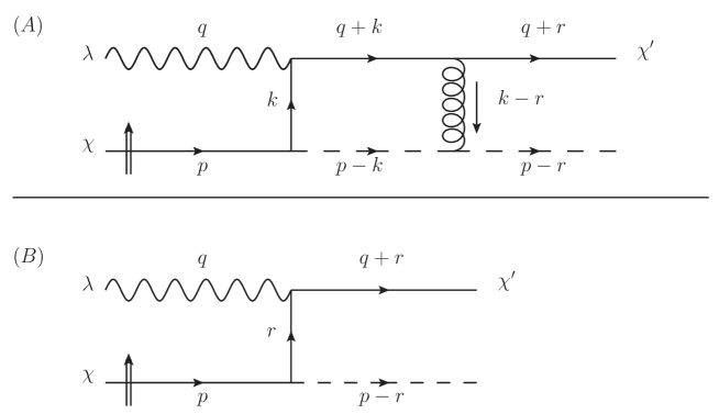
Figure 3: Diagrams for the $\gamma^{*}+p^{\uparrow}\rightarrow q+X$ SIDIS amplitude at one-loop order (A) and tree-level (B). The incoming solid line denotes the transversely polarized proton, which splits into a quark (outgoing solid line) and a diquark (dashed line).

With these kinematics, we can write down the one-loop amplitude shown in Fig. 3 (A) as

$$\mathcal{A}_{1}^{DIS} = -ig^{2}e_{f}GC_{f}\int\frac{d^{4}k}{(2\pi)^{4}}\times$$

$$\times \frac{\overline{U}_{\chi^{\prime}}(q+r)(2\not{p}-\not{k}-\not{r})(\not{q}+\not{k})\not{\epsilon}_{\lambda}\not{k}U_{\chi}(p)}{[k^{2}+i\epsilon]\,[(q+k)^{2}+i\epsilon]\,[(k-r)^{2}+i\epsilon]\,[(p-k)^{2}-\lambda^{2}+i\epsilon]}$$

$$= \frac{ig^{2}e_{f}GC_{F}}{2(2\pi)^{4}(p^{+})^{3}}\int\frac{dx\,dk^{-}\,d^{2}k}{x^{2}(x-\Delta)(1-x)}\times$$

$$\times \frac{\overline{U}_{\chi^{\prime}}(q+r)(2\not{p}-\not{k}-\not{r})(\not{q}+\not{k})\not{\epsilon}_{\lambda}\not{k}U_{\chi}(p)}{\left[k^{-}-\frac{\vec{k}_{\bot}^{2}-i\epsilon}{xp^{+}}\right]\left[k^{-}+q^{-}-\frac{(\vec{q}_{\bot}+\vec{k}_{\bot})^{2}-i\epsilon}{xp^{+}}\right]\left[k^{-}-r^{-}-\frac{(\vec{k}_{\bot}-\vec{r}_{\bot})^{2}-i\epsilon}{(x-\Delta)p^{+}}\right]\left[k^{-}-p^{-}+\frac{\vec{k}_{\bot}^{2}+\lambda^{2}-i\epsilon}{(1-x)p^{+}}\right]},$$

where the longitudinal momentum fraction in the loop is $k^{+}\equiv xp^{+}$ and $C_{F}=(N_{c}^{2}-1)/2N_{c}$ is the Casimir operator in the fundamental representation. Similarly, the tree-level amplitude shown in Fig. 3 (B) is

$$\mathcal{A}_{0}^{DIS}=\frac{e_{f}G}{r^{2}}\overline{U}_{\chi^{\prime}}(q+r)\not{\epsilon}_{\lambda}\not{r}U_{\chi}(p).$$ (40)

The lowest-order contribution to the spin-difference amplitude squared comes from the overlap of these diagrams and, in particular, the imaginary part of the denominators (cf. Eq. (2.2)):

$$\Delta\left|\mathcal{A}_{DIS}\right|^{2} = 2i\left[\frac{g^{2}e_{f}^{2}G^{2}C_{F}}{2(2\pi)^{4}r^{2}(p^{+})^{3}}\right]\int\frac{dx\,d^{2}k}{x^{2}(x-\Delta)(1-x)}\,\mathrm{Im}\left\{\int dk^{-}\frac{i}{\left[k^{-}-\frac{\vec{k}_{\bot}^{2}-i\epsilon}{xp^{+}}\right]}\right.$$

$$\times \left.\frac{1}{\left[k^{-}+q^{-}-\frac{(\vec{q}_{\bot}+\vec{k}_{\bot})^{2}-i\epsilon}{xp^{+}}\right]\left[k^{-}-r^{-}-\frac{(\vec{k}_{\bot}-\vec{r}_{\bot})^{2}-i\epsilon}{(x-\Delta)p^{+}}\right]\left[k^{-}-p^{-}+\frac{\vec{k}_{\bot}^{2}+\lambda^{2}-i\epsilon}{(1-x)p^{+}}\right]}\right\}$$

$$\times \sum_{\chi^{\prime},\lambda}\left[\overline{U}_{\chi}(p)\not{r}\not{\epsilon}^{*}_{\lambda}U_{\chi^{\prime}}(q+r)\overline{U}_{\chi^{\prime}}(q+r)(2\not{p}-\not{k}-\not{r})(\not{q}+\not{k})\not{\epsilon}_{\lambda}\not{k}U_{\chi}(p)-(\chi\rightarrow-\chi)\right]$$

where we sum over the spin of the outgoing quark and use

$$\sum_{\lambda}\epsilon^{*\,\mu}_{\lambda}(q)\,\epsilon^{\nu}_{\lambda}(q)\rightarrow-g^{\mu\nu}.$$ (42)

We will provide a justification for summing over photon polarizations in the two paragraphs following Eq. (79). Performing these sums and simplifying the expression gives

$$\Delta\left|\mathcal{A}_{DIS}\right|^{2} = \frac{2ig^{2}e_{f}^{2}G^{2}C_{F}}{(2\pi)^{4}r^{2}(p^{+})^{3}}\int\frac{dx\,d^{2}k}{x^{2}(x-\Delta)(1-x)}\,\mathcal{I}\,$$

$$\times \bigg{[}\overline{U}_{\chi}(p)\not{r}(\not{q}+\not{k})(2\not{p}-\not{k}-\not{r})(\not{q}+\not{r})\not{k}U_{\chi}(p)\,-\,(\chi\rightarrow-\chi)\bigg{]}$$

where the imaginary part that is essential for generating the asymmetry comes from the expression

$$\mathcal{I}\equiv\mathrm{Im}\!\left\{\!\int\!\!\frac{i\;dk^{-}}{\left[k^{-}-\frac{\vec{k}_{\bot}^{2}-i\epsilon}{xp^{+}}\right]\!\!\left[k^{-}+q^{-}-\frac{(\vec{q}_{\bot}+\vec{k}_{\bot})^{2}-i\epsilon}{xp^{+}}\right]\!\!\left[k^{-}-r^{-}-\frac{(\vec{k}_{\bot}-\vec{r}_{\bot})^{2}-i\epsilon}{(x-\Delta)p^{+}}\right]\!\!\left[k^{-}-p^{-}+\frac{\vec{k}_{\bot}^{2}+\lambda^{2}-i\epsilon}{(1-x)p^{+}}\right]}\!\right\}\!.$$ (44)

Notice that the numerator in (3.1) containing the Dirac matrix element is $k^{-}$-dependent, such that the $dk^{-}$ integration contained in $\mathcal{I}$ from Eq. (44) applies to it too. Superficially the numerator of (3.1) could scale as $(k^{-})^{3}$ at large $k^{-}$, which would endanger convergence; however, it actually only scales as $(k^{-})^{2}$ since $(\gamma^{+})^{2}=0$. Thus the $k^{-}$ integral scales at most as $dk^{-}/(k^{-})^{2}$, which converges and allows us to close the contour in either the upper or the lower half-plane.

In addition, we will demonstrate below that in the kinematic limit at hand given by Eq. (36) the leading contribution to the Dirac matrix element in Eq. (3.1) is, in fact, $k^{-}$-independent. We will, therefore, proceed under the assumption that this is the case and that all the $k^{-}$ dependence in (3.1) is contained in the integrand of Eq. (44), evaluating the integration in (44) separately.

The imaginary part in (44) comes from the denominators, which corresponds to putting two of the loop propagators on shell: one occurs from the residue of the $dk^{-}$ integral and the other occurs by taking the imaginary part. However, there are strong kinematic constraints that restrict which combinations of propagators can go on-shell simultaneously. We are working in the limit of massless quarks, and $1\leftrightarrow 2$ processes for on-shell massless particles are forbidden by four-momentum conservation; cuts corresponding to such processes will explicitly be impossible to put on shell. Other cuts correspond to spontaneous proton decay; proton stability against decay through various channels must be imposed by hand, resulting in kinematic constraints on the masses of the proton and the scalar.

Eq. (44) is evaluated in Appendix A. The result reads

$$\mathcal{I}=\frac{2\pi^{2}\Delta^{2}p^{+}}{Q^{2}}\frac{\delta\left[x-\left(1+2\frac{\vec{q}_{\bot}\cdot(\vec{k}_{\bot}-\vec{r}_{\bot})}{Q^{2}}\right)\Delta\right]}{\left[p^{-}-\frac{\vec{k}_{\bot}^{2}+\lambda^{2}}{(1-x)p^{+}}-\frac{\vec{k}_{\bot}^{2}}{xp^{+}}\right]\left[p^{-}-r^{-}-\frac{\vec{k}_{\bot}^{2}+\lambda^{2}}{(1-x)p^{+}}+\frac{(\vec{k}_{\bot}-\vec{r}_{\bot})^{2}}{(\Delta-x)p^{+}}\right]}.$$ (45)

Substituting this expression back into (3.1) and integrating over the delta function which sets $x\approx\Delta$ gives

$$\Delta\left|\mathcal{A}_{DIS}\right|^{2} =-ig^{2}e_{f}^{2}G^{2}C_{F}\left(\frac{\Delta(1-\Delta)}{Q^{2}(\vec{r}_{\bot}^{2}+a^{2})}\right)\int\frac{d^{2}k}{(2\pi)^{2}}\times$$ (46)

$$\times\,\frac{\overline{U}_{\chi}(p)\not{r}(\not{q}+\not{k})(2\not{p}-\not{k}-\not{r})(\not{q}+\not{r})\not{k}U_{\chi}(p)-(\chi\rightarrow-\chi)}{(\vec{k}_{\bot}-\vec{r}_{\bot})^{2}(\vec{k}_{\bot}^{2}+a^{2})},$$

where the mass parameter $a^{2}$ that regulates the infrared divergence

$$a^{2}\equiv\Delta\left(\lambda^{2}-(1-\Delta)M^{2}\right)>0$$ (47)

is ensured to be positive definite by the proton stability conditions (A3) and (A7), and we have used

$$r^{2}=\Delta\left(M^{2}-\frac{\vec{r}_{\bot}^{2}+\lambda^{2}}{1-\Delta}\right)-\vec{r}_{\bot}^{2}=-\frac{\vec{r}_{\bot}^{2}+a^{2}}{1-\Delta}.$$ (48)

Note that making this cut has fixed the loop momentum $k^{\mu}$ to be

$$k^{\mu}=\left(\Delta p^{+}\,,\,\frac{M^{2}}{p^{+}}-\frac{\vec{k}_{\bot}^{2}+\lambda^{2}}{(1-\Delta)p^{+}}\,,\,\vec{k}_{\bot}\right).$$ (49)

Next we need to evaluate the numerator of (46) by computing the difference between the matrix elements:

$$N_{DIS}=\overline{U}_{\chi}(p)\not{r}(\not{q}+\not{k})(2\not{p}-\not{k}-\not{r})(\not{q}+\not{r})\not{k}U_{\chi}(p)-(\chi\rightarrow-\chi).$$ (50)

The momenta involved in this spinor product obey the scale hierarchy

$$\overbrace{p^{+},r^{+},k^{+},q^{-},|\vec{q}_{\bot}|}^{\mathcal{O}(Q)}\,\gg\,\overbrace{|\vec{r}_{\bot}|,|\vec{k}_{\bot}|,M,\lambda}^{\mathcal{O}(\bot)}\,\gg\,\overbrace{p^{-},r^{-},k^{-}}^{\mathcal{O}\left(\bot^{2}/Q\right)},$$ (51)

with the dominant power-counting of the spin-dependent part of the Dirac matrix element being $\mathcal{O}(Q^{4}\bot^{2})$. Evaluation of $N_{DIS}$ in Eq. (50) in the kinematics of Eq. (51) is somewhat involved: after some algebra one can show that there are three classes of Dirac structures that give a contribution of the leading order, $\mathcal{O}(Q^{4}\bot^{2})$; all three involve taking the $\mathcal{O}(Q)$ momenta from the middle three gamma matrices:

$$N_{DIS} =\frac{1}{8}\left[(2p^{+}-k^{+}-r^{+})(q^{-})^{2}\right]\,\overline{U}_{\chi}(p)\,\not{r}\gamma^{+}\gamma^{-}\gamma^{+}\not{k}\,U_{\chi}(p)-(\chi\rightarrow-\chi)$$ (52)

$$=\left[(1-\Delta)p^{+}(q^{-})^{2}\right]\,\overline{U}_{\chi}(p)\,\not{r}\gamma^{+}\not{k}\,U_{\chi}(p)-(\chi\rightarrow-\chi).$$

The three variations consist of taking $\gamma^{-}$ for both $\not{r}$ and $\not{k}$, taking $\gamma^{-}$ for one and $\gamma_{\bot}$ for the other, or taking $\gamma_{\bot}$ for both.

In the first case, if we take $\gamma^{-}$ for both $\not{r}$ and $\not{k}$, we obtain

$$\overline{U}_{\chi}(p)\,\not{r}\gamma^{+}\not{k}\,U_{\chi}(p) \rightarrow \frac{1}{4}\Delta^{2}(p^{+})^{2}\,\overline{U}_{\chi}(p)\,\gamma^{-}\gamma^{+}\gamma^{-}\,U_{\chi}(p)$$

$$= \Delta^{2}(p^{+})^{2}\,\overline{U}_{\chi}(p)\,\gamma^{-}\,U_{\chi}(p),$$

but $\overline{U}_{\chi}(p)\,\gamma^{-}\,U_{\chi}(p)=\frac{2M^{2}}{p^{+}}$ is spin-independent and cannot generate the asymmetry. Similarly, if we take $\gamma_{\bot}$ for both $\not{r}$ and $\not{k}$, we obtain

$$\overline{U}_{\chi}(p)\,\not{r}\gamma^{+}\not{k}\,U_{\chi}(p) \rightarrow r_{\bot}^{i}k_{\bot}^{j}\overline{U}_{\chi}(p)\,\gamma_{\bot}^{i}\gamma^{+}\gamma_{\bot}^{j}\,U_{\chi}(p),$$ (54)

but $\overline{U}_{\chi}(p)\,\gamma_{\bot}^{i}\gamma^{+}\gamma_{\bot}^{j}\,U_{\chi}(p)=2p^{+}\delta^{ij}$ is also spin-independent and cannot generate the asymmetry. However, if we take one each of $\gamma_{\bot}$ and $\gamma^{-}$, we obtain

$$\overline{U}_{\chi}(p)\,\not{r}\gamma^{+}\not{k}\,U_{\chi}(p) \rightarrow -\frac{1}{2}\Delta p^{+}\bigg{[}r_{\bot}^{i}\overline{U}_{\chi}(p)\,\gamma_{\bot}^{i}\gamma^{+}\gamma^{-}\,U_{\chi}(p)+$$

$$+ k_{\bot}^{i}\overline{U}_{\chi}(p)\,\gamma^{-}\gamma^{+}\gamma_{\bot}^{i}\,U_{\chi}(p)\bigg{]}.$$

We can further simplify this expression by using the Dirac equation

$$0=(\not{p}-M)U_{\chi}(p)=\left[\frac{1}{2}p^{+}\gamma^{-}+\frac{M^{2}}{2p^{+}}\gamma^{+}-M\right]U_{\chi}(p)$$ (56)

to rewrite the action of $\gamma^{-}$ in terms of $\gamma^{+}$ and $M$. Since $(\gamma^{+})^{2}=0$, this simplifies (3.1) to

$$\overline{U}_{\chi}(p)\,\not{r}\gamma^{+}\not{k}\,U_{\chi}(p) \rightarrow -M\Delta(k_{\bot}^{i}-r_{\bot}^{i})\,\overline{U}_{\chi}(p)\,\gamma^{+}\gamma_{\bot}^{i}\,U_{\chi}(p),$$ (57)

and $\overline{U}_{\chi}(p)\,\gamma^{+}\gamma_{\bot}^{i}\,U_{\chi}(p)=2i\chi p^{+}\delta^{i2}$, which is spin-dependent and generates the asymmetry. Altogether this gives

$$N_{DIS} = -2i\chi\Delta(1-\Delta)(p^{+})^{2}(q^{-})^{2}M(k_{\bot}^{(2)}-r_{\bot}^{(2)})-(\chi\rightarrow-\chi)$$

$$= -4i\left(\frac{1-\Delta}{\Delta}\right)Q^{4}M(k_{\bot}^{(2)}-r_{\bot}^{(2)}),$$

so that the spin-difference matrix element is pure imaginary, as was proved in (27).

Substituting this result back into (46) gives (cf. Eq. (31) in [27])

$$\Delta\left|\mathcal{A}_{DIS}\right|^{2} =-4g^{2}e_{f}^{2}G^{2}C_{F}\left(\frac{(1-\Delta)^{2}Q^{2}M}{\vec{r}_{\bot}^{2}+a^{2}}\right)\int\frac{d^{2}k}{(2\pi)^{2}}\frac{k_{\bot}^{(2)}-r_{\bot}^{(2)}}{(\vec{k}_{\bot}-\vec{r}_{\bot})^{2}\,(\vec{k}_{\bot}^{2}+a^{2})}$$

$$=+\frac{g^{2}e_{f}^{2}G^{2}C_{F}}{\pi}(1-\Delta)^{2}\frac{Q^{2}Mr_{\bot}^{(2)}}{\vec{r}_{\bot}^{2}(\vec{r}_{\bot}^{2}+a^{2})}\ln\left(\frac{\vec{r}_{\bot}^{2}+a^{2}}{a^{2}}\right),$$ (59)

where the $d^{2}k$ integral is performed using Feynman parameters obtaining

$$\int\frac{d^{2}k}{(2\pi)^{2}}\frac{k_{\bot}^{(2)}-r_{\bot}^{(2)}}{(\vec{k}_{\bot}-\vec{r}_{\bot})^{2}\,(\vec{k}_{\bot}^{2}+a^{2})}=-\frac{1}{4\,\pi}\,\frac{r_{\bot}^{(2)}}{\vec{r}_{\bot}^{2}}\,\ln\left(\frac{\vec{r}_{\bot}^{2}+a^{2}}{a^{2}}\right).$$ (60)

Eq. (59) is the final expression for the spin-difference amplitude squared for deep inelastic scattering. We would next like to compare this expression with the result for the Drell-Yan process.

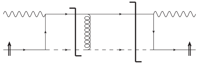
Figure 4: Diagrammatic representation of the origin of complex phase leading to the single-spin asymmetry in SIDIS. The longer cut denotes the final state of the process, while the shorter cut demonstrates the origin of the phase needed for the asymmetry.

Before we do that, let us stress once again that the asymmetry in the SIDIS case arises from the contribution of the diagram in Fig. 3 (A) with the $(q+k)$- and $(p-k)$-lines (corresponding to the lines labeled ④ and ② in Appendix A) which are put on mass-shell. It is this and only this contribution that gives the imaginary phase needed for the asymmetry in SIDIS. This fact becomes more apparent if we diagrammatically represent putting the $(q+k)$- and $(p-k)$-lines on mass-shell by a cut, as shown in Fig. 4. In Fig. 4 we show the amplitude squared which we have just calculated, with the longer cut representing the true final state of the process, and the shorter vertical cut line representing the imaginary phase generating the asymmetry. The shorter cut follows the standard Cutkosky rules [46], with the caveat stressed above in Sec. 2.2 that it should not be applied to the spinor matrix element; that is, the shorter cut applies to the denominators of the propagators only, as if we are evaluating the diagram in a scalar field theory. Using the Cutkosky rules one can clearly see that this is the only way the shorter cut line can be placed in the diagram, as all other cuts would lead to various prohibited $1\to 2$ or $2\to 1$ processes, including proton decay. Thus Fig. 4 demonstrates that the imaginary phase needed for the single-spin asymmetry arises only in diagrams where it is possible to place a second cut. We will make use of this result in the analysis of the Drell-Yan process below.

3.2 Drell-Yan Process

We now perform a similar calculation for the Drell-Yan process in the same model considered above for deep inelastic scattering. We will consider the scattering of an antiquark on a transversely-polarized proton with transverse spin eigenvalue $\chi$ that produces a virtual photon, which then decays into a dilepton pair with invariant mass $q^{2}=Q^{2}$. This process is shown in Fig. 5 at the level of virtual photon production: $\overline{q}+p^{\uparrow}\rightarrow\gamma^{*}+X$.

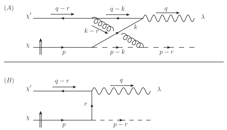
Figure 5: Diagrams for the $\overline{q}+p^{\uparrow}\rightarrow\gamma^{*}+X$ DY amplitude at one-loop order (A) and tree-level (B). The incoming proton and anti-quark are denoted by the lower and upper solid lines correspondingly, with the outgoing diquark denoted by the dashed line.

Following [9], we work in a generic frame collinear to the proton ($\vec{p}_{\bot}=\vec{0}_{\bot}$). We define the longitudinal momentum fraction of the photon to be $\beta\equiv q^{+}/p^{+}$ and the momentum fraction exchanged in the t-channel to be $\Delta\equiv r^{+}/p^{+}$. As before, four-momentum conservation and the on-shell conditions fix $r^{-}$ and $q^{-}$ to be

$$r^{-} = p^{-}-(p-r)^{-}=\frac{M^{2}}{p^{+}}-\frac{\vec{r}_{\bot}^{2}+\lambda^{2}}{(1-\Delta)p^{+}}$$ (61)

$$q^{-} = (q-r)^{-}+r^{-}=\frac{(\vec{q}_{\bot}-\vec{r}_{\bot})^{2}}{(\beta-\Delta)p^{+}}+r^{-}\approx\frac{\vec{q}_{\bot}^{2}-2\vec{q}_{\bot}\cdot\vec{r}_{\bot}}{(\beta-\Delta)p^{+}}+\mathcal{O}\left(\frac{\bot^{2}}{p^{+}}\right).$$

In this frame, the virtual photon’s large invariant mass $Q^{2}$ comes in part from its transverse components and in part from its longitudinal components:

$$Q^{2}\equiv q^{2}=\beta p^{+}q^{-}-\vec{q}_{\bot}^{2}\approx\left(\frac{\Delta}{\beta-\Delta}\right)\vec{q}_{\bot}^{2}+\mathcal{O}\left(\frac{\bot}{Q}\right).$$ (62)

This allows us to approximate $q^{-}$ as

$$q^{-}\approx\frac{Q^{2}}{\Delta p^{+}}+\mathcal{O}\left(\frac{Q\bot}{p^{+}}\right),$$ (63)

which agrees with the corresponding expression (37) for DIS to leading order in $Q^{2}$. The kinematics can be summarized as

$$p^{\mu} =\left(p^{+}\,,\,\frac{M^{2}}{p^{+}}\,,\,\vec{0}_{\bot}\right)$$ (64)

$$q^{\mu} =\left(\beta p^{+}\,,\,\frac{(\vec{q}_{\bot}-\vec{r}_{\bot})^{2}}{(\beta-\Delta)p^{+}}+\frac{M^{2}}{p^{+}}-\frac{\vec{r}_{\bot}^{2}+\lambda^{2}}{(1-\Delta)p^{+}}\,,\,\vec{q}_{\bot}\right)$$

$$r^{\mu} =\left(\Delta p^{+}\,,\,\frac{M^{2}}{p^{+}}-\frac{\vec{r}_{\bot}^{2}+\lambda^{2}}{(1-\Delta)p^{+}}\,,\,\vec{r}_{\bot}\right).$$

Notice that, in this frame, the on-shell conditions for the antiquark, scalar, and dilepton pair imply that $(\beta-\Delta)>0,\beta>0,$ and $(1-\Delta)>0$. Additionally, to leading order, the positivity constraint on $q^{-}$ (63) implies that $\Delta>0$, and we can choose our frame such that $\beta<1$, although this is not strictly necessary. Altogether, this gives a hierarchy of the fixed scales to be $0<\Delta<\beta<1$.

With these kinematics, we can evaluate the one-loop amplitude shown in Fig. 5 (A) as

$$\mathcal{A}_{1}^{DY} = \frac{ig^{2}e_{f}GC_{F}}{(2\pi)^{4}}\int d^{4}{k}\frac{\overline{V}_{\chi^{\prime}}(q-r)(2\not{p}-\not{k}-\not{r})(\not{k}-\not{q})\not{\epsilon}^{*}_{\lambda}\not{k}U_{\chi}(p)}{\left[k^{2}+i\epsilon\right]\left[(k-q)^{2}+i\epsilon\right]\left[(k-r)^{2}+i\epsilon\right]\left[(p-k)^{2}-\lambda^{2}+i\epsilon\right]}$$

$$= \frac{-ig^{2}e_{f}GC_{F}}{2(2\pi)^{4}(p^{+})^{3}}\int\frac{dx\,dk^{-}\,d^{2}k}{x(x-\beta)(x-\Delta)(1-x)}\times$$

$$\times \frac{\overline{V}_{\chi^{\prime}}(q-r)(2\not{p}-\not{k}-\not{r})(\not{k}-\not{q})\not{\epsilon}_{\lambda}^{*}\not{k}U_{\chi}(p)}{\left[k^{-}-\frac{\vec{k}_{\bot}^{2}-i\epsilon}{xp^{+}}\right]\left[k^{-}-q^{-}-\frac{(\vec{k}_{\bot}-\vec{q}_{\bot})^{2}-i\epsilon}{(x-\beta)p^{+}}\right]\left[k^{-}-r^{-}-\frac{(\vec{k}_{\bot}-\vec{r}_{\bot})^{2}-i\epsilon}{(x-\Delta)p^{+}}\right]\left[k^{-}-p^{-}+\frac{\vec{k}_{\bot}^{2}+\lambda^{2}-i\epsilon}{(1-x)p^{+}}\right]},$$

where $x\equiv k^{+}/p^{+}$ is the longitudinal momentum fraction in the loop. Similarly, the tree-level amplitude shown in Fig. 5 (B) is

$$\mathcal{A}_{0}^{DY}=-\frac{e_{f}G}{r^{2}}\overline{V}_{\chi^{\prime}}(q-r)\not{\epsilon}_{\lambda}^{*}\not{r}U_{\chi}(p).$$ (66)

This allows us to calculate the spin-difference amplitude squared following (2.2) as

$$\Delta|\mathcal{A}_{DY}|^{2} = 2i\left[\frac{g^{2}e_{f}^{2}G^{2}C_{F}}{2(2\pi)^{4}(p^{+})^{3}r^{2}}\right]\int\frac{dx\,d^{2}k}{x(x-\beta)(x-\Delta)(1-x)}\mathrm{Im}\left\{\int dk^{-}\frac{i}{\left[k^{-}-\frac{\vec{k}_{\bot}^{2}-i\epsilon}{xp^{+}}\right]}\right.$$

$$\times \left.\frac{1}{\left[k^{-}-q^{-}-\frac{(\vec{k}_{\bot}-\vec{q}_{\bot})^{2}-i\epsilon}{(x-\beta)p^{+}}\right]\left[k^{-}-r^{-}-\frac{(\vec{k}_{\bot}-\vec{r}_{\bot})^{2}-i\epsilon}{(x-\Delta)p^{+}}\right]\left[k^{-}-p^{-}+\frac{\vec{k}_{\bot}^{2}+\lambda^{2}-i\epsilon}{(1-x)p^{+}}\right]}\right\}$$

$$\times \sum_{\chi^{\prime},\lambda}\left[\overline{U}_{\chi}(p)\,\not{r}\not{\epsilon}_{\lambda}V_{\chi^{\prime}}(q-r)\overline{V}_{\chi^{\prime}}(q-r)(2\not{p}-\not{k}-\not{r})(\not{k}-\not{q})\not{\epsilon}_{\lambda}^{*}\not{k}\,U_{\chi}(p)-(\chi\rightarrow-\chi)\right]$$

where we sum over the spin of the incoming antiquark and use Eq. (42). (See the discussion following Eq. (79) for a justification of summing over photon polarizations.) Performing these sums and simplifying the result gives

$$\Delta|\mathcal{A}_{DY}|^{2} =\frac{2ig^{2}e_{f}^{2}G^{2}C_{F}}{(2\pi)^{4}r^{2}(p^{+})^{3}}\int\frac{dx\,d^{2}k}{x(x-\beta)(x-\Delta)(1-x)}\,\mathcal{I}$$ (68)

$$\times\,\left[\overline{U}_{\chi}(p)\,\not{r}(\not{k}-\not{q})(2\not{p}-\not{k}-\not{r})(\not{q}-\not{r})\not{k}\,U_{\chi}(p)-(\chi\rightarrow-\chi)\right],$$

where the imaginary part necessary for the asymmetry is generated by

$$\mathcal{I}\equiv\mathrm{Im}\!\left\{\!\int\!\!\frac{i\;dk^{-}}{\left[k^{-}-\frac{\vec{k}_{\bot}^{2}-i\epsilon}{xp^{+}}\right]\!\!\left[k^{-}-q^{-}-\frac{(\vec{k}_{\bot}-\vec{q}_{\bot})^{2}-i\epsilon}{(x-\beta)p^{+}}\right]\!\!\left[k^{-}-r^{-}-\frac{(\vec{k}_{\bot}-\vec{r}_{\bot})^{2}-i\epsilon}{(x-\Delta)p^{+}}\right]\!\!\left[k^{-}-p^{-}+\frac{\vec{k}_{\bot}^{2}+\lambda^{2}-i\epsilon}{(1-x)p^{+}}\right]}\!\right\}\!.$$ (69)

As before, the imaginary part (69) corresponds to putting two of the loop propagators on-shell simultaneously: one from performing the $k^{-}$ integral and another from taking the imaginary part. The propagators that can be simultaneously put on-shell are strongly constrained by the kinematics and by the requirement of proton stability. The expression (69) is evaluated in Appendix B yielding

$$\mathcal{I}=\frac{2\pi^{2}\Delta(\beta-\Delta)p^{+}}{Q^{2}}\frac{\delta\left[x-\left(1+2\,\frac{\vec{q}_{\bot}\cdot(\vec{k}_{\bot}-\vec{r}_{\bot})}{Q^{2}}\right)\Delta\right]}{\left[\frac{\vec{k}_{\bot}^{2}}{xp^{+}}-r^{-}+\frac{(\vec{k}_{\bot}-\vec{r}_{\bot})^{2}}{(\Delta-x)p^{+}}\right]\left[\frac{\vec{k}_{\bot}^{2}}{xp^{+}}-p^{-}+\frac{\vec{k}_{\bot}^{2}+\lambda^{2}}{(1-x)p^{+}}\right]},$$ (70)

which we can substitute back into (68). Integrating over the delta function sets $x\approx\Delta$, giving

$$\Delta|\mathcal{A}_{DY}|^{2} =-ig^{2}e_{f}^{2}G^{2}C_{F}\left(\frac{\Delta(1-\Delta)}{Q^{2}(\vec{r}_{\bot}^{2}+a^{2})}\right)\int\frac{d^{2}k}{(2\pi)^{2}}$$ (71)

$$\times\frac{\overline{U}_{\chi}(p)\,\not{r}(\not{k}-\not{q})(2\not{p}-\not{k}-\not{r})(\not{q}-\not{r})\not{k}\,U_{\chi}(p)-(\chi\rightarrow-\chi)}{(\vec{k}_{\bot}-\vec{r}_{\bot})^{2}\,(\vec{k}_{\bot}^{2}+a^{2})},$$

where we have again employed (47) and (48), since we have established that the proton stability constraint (A3) is still valid for the Drell-Yan process. In performing the longitudinal integrals, we have fixed the loop momentum $k^{\mu}$ to be

$$k^{\mu}=\left(\Delta p^{+}\,,\,\frac{\vec{k}_{\bot}^{2}}{\Delta p^{+}}\,,\,\vec{k}_{\bot}\right).$$ (72)

Comparison of (46) with (71) shows that the only difference between the two processes occurs in the numerators, rather than in the denominators. The essential difference in the numerators is the reversal of the intermediate (anti)quark propagator from $\not{q}+\not{k}$ in deep inelastic scattering to $\not{k}-\not{q}$ in the Drell-Yan process. We will return to this point later in the analysis of the results.

Next we need to evaluate the spin-difference matrix element appearing in the numerator of (71):

$$N_{DY}=\overline{U}_{\chi}(p)\,\not{r}(\not{k}-\not{q})(2\not{p}-\not{k}-\not{r})(\not{q}-\not{r})\not{k}\,U_{\chi}(p)-(\chi\rightarrow-\chi).$$ (73)

The momenta obey the same scale hierarchy (51) as in deep inelastic scattering, with the addition of $q^{+}$ as a scale at $\mathcal{O}(Q)$ in our frame for Drell-Yan. The other momenta can differ from their values in DIS by factors of $\mathcal{O}(1)$, but the power-counting is the same. Again, the dominant power-counting of the matrix element is $\mathcal{O}(Q^{4}\bot^{2})$, which only arises from taking

$$(\not{k}-\not{q})(2\not{p}-\not{k}-\not{r})(\not{q}-\not{r}) \rightarrow \ -\frac{1}{8}(q^{-})^{2}(2p^{+}-k^{+}-r^{+})\,\gamma^{+}\gamma^{-}\gamma^{+}$$

$$= -(1-\Delta)(p^{+})(q^{-})^{2}\gamma^{+}$$

so that

$$N_{DY}=-\left[(1-\Delta)p^{+}(q^{-})^{2}\right]\,\overline{U}_{\chi}(p)\,\not{r}\gamma^{+}\not{k}\,U_{\chi}(p)-(\chi\rightarrow-\chi).$$ (75)

Comparing (75) with (52), we see that

$$N_{DY}=-N_{DIS}$$ (76)

to leading order in $Q$, so we can immediately write the numerator for Drell-Yan using (3.1) as

$$N_{DY}=+4i\left(\frac{1-\Delta}{\Delta}\right)Q^{4}M(k_{\bot}^{(2)}-r_{\bot}^{(2)}).$$ (77)

Substituting this back into (71) yields the same transverse momentum integral as in DIS, which we can evaluate using Feynman parameters to obtain the final answer

$$\Delta|\mathcal{A}_{DY}|^{2} =-\frac{g^{2}e_{f}^{2}G^{2}C_{F}}{\pi}(1-\Delta)^{2}\frac{Q^{2}Mr_{\bot}^{(2)}}{\vec{r}_{\bot}^{2}(\vec{r}_{\bot}^{2}+a^{2})}\,\ln\left(\frac{\vec{r}_{\bot}^{2}+a^{2}}{a^{2}}\right)$$ (78)

$$=-\Delta|\mathcal{A}_{DIS}|^{2}.$$

Thus we conclude that the spin-difference amplitude squared from the Drell-Yan process is exactly the negative of the that from deep inelastic scattering, (59).

To obtain the single-spin asymmetry $A_{N}$ one needs to divide $\Delta|\mathcal{A}|^{2}$ for DY and SIDIS by twice the unpolarized amplitude squared (averaged over the incoming proton polarizations), as follows from Eq. (28). Both in the SIDIS and DY cases the unpolarized amplitude squared is dominated by the Born-level processes, with the amplitudes given in Eqs. (40) and (66) correspondingly. One can easily show that the squares of those amplitudes, averaged over the proton polarizations, are, in fact, equal, such that Eq. (78) leads to [8, 9]

$$A_{N}^{DY}=-A_{N}^{DIS}.$$ (79)

The sign-reversal has also been derived in [8] for the SIDIS and DY Sivers functions [6, 7, 8, 36]. At the same time in our analysis we have studied the full SIDIS and DY processes (cf. [4, 9]) instead of the corresponding Sivers functions. However, the conclusion (79) was reached using Eq. (42) above: in particular, note that we have reduced the SIDIS process to $\gamma^{*}+p^{\uparrow}\to q+X$ scattering and have summed over polarizations of the incoming virtual photon. This is not an exact representation of the physical SIDIS process, since we have to convolute the hadronic interaction part of the diagram with a lepton tensor coming from the electron-photon interactions. Likewise, for the Drell-Yan process we have replaced the second hadron by an anti-quark, reducing it to the $q+p^{\uparrow}\to\gamma^{*}+X$ scattering. (Replacing the $l^{+}l^{-}$-pair by a time-like photon is also an approximation, true up to an overall multiplicative factor due to current conservation.) The resolution for these questions is in the fact that, in the eikonal kinematics (36) considered, the single-spin asymmetries in the $\gamma^{*}+p^{\uparrow}\to q+X$ and $q+p^{\uparrow}\to\gamma^{*}+X$ processes are proportional to the Sivers functions for SIDIS and DY correspondingly, as can be shown along the lines of [27].

Consider the quark correlator in a proton [47, 27]

$$\Phi_{ij}(\Delta,{\vec{r}}_{\perp};P,S)\equiv\int\frac{dx^{-}\,d^{2}x_{\perp}}{(2\,\pi)^{3}}\,e^{i\,\left(\frac{1}{2}\,x\,p^{+}\,x^{-}-{\vec{x}}_{\perp}\cdot{\vec{r}}_{\perp}\right)}\,\langle P,S|{\bar{\psi}}_{j}(0)\,{\cal U}\,\psi_{i}(x^{+}=0,x^{-},{\vec{x}}_{\perp})|P,S\rangle,$$ (80)

where the quark has transverse momentum ${\vec{r}}_{\perp}$ and the longitudinal momentum fraction $\Delta$, the proton spin four-vector is $S^{\mu}$, while ${\cal U}$ is the gauge link necessary to make the object gauge-invariant. The correlation function $\Phi_{ij}$ can be decomposed as [19, 27]

$$\Phi_{ij}(\Delta,{\vec{r}}_{\perp};P,S)=\frac{M}{2\,p^{+}}\,\bigg{[}f_{1}(\Delta,{\vec{r}}_{\perp})\,\frac{\not{p}}{M}+\frac{1}{M^{2}}\,f_{1\,T}^{\perp}(\Delta,{\vec{r}}_{\perp})\,\epsilon_{\mu\nu\rho\sigma}\,\gamma^{\mu}\,p^{\nu}\,r_{\perp}^{\rho}\,S_{T}^{\sigma}-\frac{1}{M}\,q_{1s}(\Delta,{\vec{r}}_{\perp})\,\not{p}\,\gamma^{5}$$

$$-\frac{1}{M}\,h_{1T}(\Delta,{\vec{r}}_{\perp})\,i\,\sigma_{\mu\nu}\,\gamma^{5}\,S_{T}^{\mu}\,p^{\nu}-\frac{1}{M^{2}}\,h_{1s}^{\perp}(\Delta,{\vec{r}}_{\perp})\,i\,\sigma_{\mu\nu}\,\gamma^{5}\,r_{\perp}^{\mu}\,p^{\nu}+h_{1}^{\perp}(\Delta,{\vec{r}}_{\perp})\,\sigma_{\mu\nu}\,\frac{r_{\perp}^{\mu}\,p^{\nu}}{M^{2}}\bigg{]}_{ij}.$$ (81)

The Sivers function $f_{1\,T}^{\perp}(\Delta,{\vec{r}}_{\perp})$ can be singled out by extracting the spin-dependent part of $\Phi_{ij}(\gamma^{+})_{ji}$, that is [27]

$$\Phi_{ij}(\gamma^{+})_{ji}\bigg{|}_{\text{spin dependent}}=\frac{2}{M}\,\epsilon^{ij}\,S_{T}^{i}\,r_{\perp}^{j}\,f_{1\,T}^{\perp}(\Delta,{\vec{r}}_{\perp}).$$ (82)

Comparing Eq. (82) to Eqs. (52) and (75) above (and comparing the latter two equations to Eq. (29) in [27]) we see that both calculation performed here for the SIDIS and DY processes single out the corresponding Sivers functions. In fact our calculation is consistent with that performed in [27], as can be seen by comparing Eqs. (59) and (78) to Eq. (31) in [27]. We can understand this consistency from the fact that the summing over the polarization of the virtual photon after Eq. (3.1) and (3.2) (see Eq. (42)) corresponds to replacing $\gamma^{+}$ in the left hand side of Eq. (82) by $\gamma_{\mu}\gamma^{+}\gamma^{\mu}$ which is just $-2\gamma^{+}$. Thus the contributions of both Eqs. (59) and (78) are proportional to the SIDIS and DY Sivers functions, calculated in the particular model for the proton considered here, with, as one can show, identical proportionality coefficients. (This point is strengthened further by noticing that the relation in Eq. (78) is only valid if one writes the spin-difference amplitudes in terms of $Q^{2}$ and $\Delta=x_{F}$, as is proper for the distribution function like a Sivers function.) Therefore, the sign reversal in Eq. (79) is just an explicit manifestation of the sign reversal between the SIDIS and DY Sivers functions.

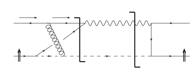
Figure 6: Diagrammatic representation of the origin of complex phase leading to the single-spin asymmetry in the Drell-Yan process. The longer cut denotes the final state of the process, while the shorter cut demonstrates the origin of the phase needed for the asymmetry.

It is interesting to investigate the diagrammatic origin of the sign-flip in Eqs. (78) and (79). To do that we consider the diagram contributing to the single-spin asymmetry in the Drell-Yan process shown in Fig. 6. As follows from the calculation in Appendix B, the asymmetry in the Drell-Yan case arises due to putting the $(q-k)$- and $k$-lines in Fig. 5 (A) (corresponding to lines ① and ② in Figs. 13 and 14) on mass-shell: this is illustrated in Fig. 6 by the second (shorter) cut, in analogy to Fig. 4. Comparing Figures 6 and 4, we see that the minus sign in Eqs. (78) and (79) arises due to the replacement of the outgoing eikonal quark in Fig. 4 by the incoming eikonal anti-quark in Fig. 6: this is in complete analogy with the original Wilson-line time-reversal argument of Collins [8] (see also [36]).

However, a closer inspection of Figures 4 and 6 reveals that the cuts generating the complex phase appear to be different: in Fig. 4 the (shorter) cut crosses the struck quark and the diquark lines, while in Fig. 6 the (shorter) cut crosses the anti-quark line and the line of the quark in the proton wave function. While we have already identified the outgoing quark/incoming anti-quark duality in SIDIS vs. DY as generating the sign flip, the fact that in the proton’s wave function the diquark is put on mass shell in SIDIS and the quark is put on mass shell in DY makes one wonder why the absolute magnitudes of the asymmetries in Eq. (79) are equal. After all, different cuts may lead to different contributions to the magnitudes of the asymmetry.

Ultimately the origin of Eq. (79) is in the fact that spin-asymmetry is a pseudo $T$-odd quantity and the Wilson lines describing the outgoing quark in SIDIS and the incoming anti-quark in DY are related by a time-reversal transformation [8]. However, in the diagrams at hand the origin of the equivalence of the shorter cuts in Figs. 4 and 6 is as follows. Consider the splitting of a polarized proton into a quark and a diquark as shown in Fig. 7: this subprocess is common to both diagrams in Figs. 4 and 6. The essential difference between Figs. 4 and 6 that we are analyzing is in the fact that in Fig. 4 the diquark is on mass shell, while in Fig. 6 the quark is on mass shell.

Figure 7: Polarized proton splitting into a quark and a diquark, which is a part of the diagrams in both Figs. 4 and 6.

Concentrating on the denominators of the quark and diquark propagators in Fig. 7 we shall write for the SIDIS case of Fig. 4 (quark is off mass shell, diquark is on mass shell)

$$\frac{1}{k^{2}}\,\delta\left((p-k)^{2}-\lambda^{2}\right)=\frac{-1}{p^{+}\,({\vec{k}}_{\perp}^{2}+a^{2})}\,\delta\left(k^{-}-\frac{M^{2}}{p^{+}}+\frac{{\vec{k}}_{\perp}^{2}+\lambda^{2}}{(1-\Delta)\,p^{+}}\right)\approx\frac{-1}{p^{+}\,({\vec{k}}_{\perp}^{2}+a^{2})}\,\delta(k^{-}),$$ (83)

where we have used Eqs. (38), (51), and (47) along with $x\approx\Delta$, and, in the last step, neglected all ${\cal O}(\perp^{2}/Q)$ terms inside the delta-function since the numerator of the diagram does not depend in the exact value of $k^{-}$ as long as it is small.

A similar calculation for the Drell-Yan process from Fig. 6 (quark is on mass shell, diquark is off mass shell in Fig. 7) employing Eqs. (64) and (51) leads to

$$\frac{1}{(p-k)^{2}-\lambda^{2}}\,\delta\left(k^{2}\right)=\frac{-1}{p^{+}\,({\vec{k}}_{\perp}^{2}+a^{2})}\,\delta\left(k^{-}-\frac{{\vec{k}}_{\perp}^{2}}{\Delta\,p^{+}}\right)\approx\frac{-1}{p^{+}\,({\vec{k}}_{\perp}^{2}+a^{2})}\,\delta(k^{-}).$$ (84)

We see that although the two contributions in Eqs. (83) and (84) are, in general, different, in the kinematics (51) they are apparently equivalent, leading to two different cuts in Figs. 4 and 6 giving the same-magnitude asymmetries.

To complete this Section, let us note that, in the framework of the model at hand, there is another diagram in the Drell-Yan process which at first glance contains both the spin-dependence and a complex phase needed to generate the single-spin asymmetry. The diagram is shown in Fig. 8 with its contribution to the single-spin asymmetry denoted by the double-cut notation of Figs. 4 and 6. The potential contribution to the asymmetry arises due to a phase generated by the correction to the quark-photon vertex in Fig. 8. Note that an analogous graph cannot give an imaginary part in the case of SIDIS, since there the virtual photon is space-like.

Figure 8: The potential contribution to the asymmetry in DY coming from the quark-photon vertex correction.

We will also demonstrate that the contribution of the diagram in Fig. 8 to the single-spin asymmetry is zero. To do this one needs to evaluate the numerator of this diagram (minus the spin-flip term):

$$\sum_{\lambda}\overline{U}_{\chi}(p)\,\not{r}\not{\epsilon}_{\lambda}(\not{q}-\not{r})\gamma^{\mu}(\not{q}-\not{k})\not{\epsilon}^{*}_{\lambda}\not{k}\gamma_{\mu}\not{r}\,U_{\chi}(p)-(\chi\rightarrow-\chi)$$

$$=-8\,k\cdot(q-r)\,\overline{U}_{\chi}(p)\,\not{r}(\not{q}-\not{k})\not{r}\,U_{\chi}(p)-(\chi\rightarrow-\chi)$$

$$=-8\,k\cdot(q-r)\,\left[2\,r\cdot(q-k)\,\overline{U}_{\chi}(p)\,\not{r}\,U_{\chi}(p)-r^{2}\,\overline{U}_{\chi}(p)\,(\not{q}-\not{k})\,U_{\chi}(p)\right]-(\chi\rightarrow-\chi)=0.$$ (85)

The zero answer results from the fact that, as can be checked explicitly, forward Dirac matrix elements of transverse spinors with a single gamma-matrix, i.e. expressions like $\overline{U}_{\chi}(p)\,\gamma^{\mu}\,U_{\chi}(p)$, are $\chi$-independent. Hence, the diagram in Fig. 8 does not contribute to the asymmetry. (In fact, the second line of Eq. (3.2) is proportional to the square of the Born term from Fig. 5 (B): as we show in Sec. 2.2 the square of the Born diagram cannot lead to a non-zero single-spin asymmetry.)

Finally, let us point out that in the calculation of the asymmetries in both SIDIS and DY, we have neglected diagrams in which the virtual photon couples to either the proton or the scalar diquark instead of the (anti)quark. These diagrams are necessary to ensure gauge invariance, but they are suppressed by powers of $\bot/Q$, which allowed us to neglect them.

4 Model Calculations with LFPTH

In this section we show that we can re-derive the results obtained in Section 3 by using light-front perturbation theory (LFPTH) [42, 43]. The LFPTH approach and covariant Feynman diagrams calculations are equivalent; however, we find it instructive to show the equivalence explicitly.

4.1 SIDIS

The LFPTH diagrams contributing to the single-spin asymmetry in SIDIS are shown in Fig. 9. Let us point out from the outset that the diagrams containing instantaneous terms do not contribute to the asymmetry in SIDIS and, therefore, are not shown in Fig. 9. This is clear from the calculation of the numerator in Sec. 3.1. The dominant contribution to the numerator comes from $\gamma^{-}$ in the quark-gluon vertex, which eliminated the possibility of the instantaneous gluon exchange contributing. The factor of $\gamma^{+}$ arising in the second line of Eq. (52) due to the photon-quark interactions eliminates the possibility of the instantaneous quark line exchanges.

Figure 9: The diagrams in LFPTH contributing to the SIDIS amplitude in Fig. 3 (A). Here labels (A) and (B) denote the diagrams corresponding to Cases A and B in Table 1.

The numerators of the amplitudes calculated in the Feynman diagram approach of Sec. 3, consisting of the Dirac matrix element and vertex factors, are clearly identical to those one would find using LFPTH. Therefore, we will only study below the energy denominators of LFPTH diagrams along with the $1/k^{+}$-factors for internal lines.

We begin our analysis with Case B from Table 1 in Appendix A, $x>\Delta$, illustrated in the diagram (B) in Fig. 9. Concentrating on the light-front energy denominators and $1/k^{+}$-factors for internal lines, we write with the help of Eq. (38)

$$\frac{1}{(k^{+})^{2}\,(p^{+}-k^{+})\,(k^{+}-r^{+})}\,\frac{1}{\left[p^{-}-\frac{\vec{k}_{\bot}^{2}}{k^{+}}-\frac{\vec{k}_{\bot}^{2}+\lambda^{2}}{p^{+}-k^{+}}+i\,\epsilon\right]\left[p^{-}+q^{-}-\frac{(\vec{k}_{\bot}+\vec{q}_{\bot})^{2}}{k^{+}}-\frac{\vec{k}_{\bot}^{2}+\lambda^{2}}{p^{+}-k^{+}}+i\,\epsilon\right]}$$

$$\times\,\frac{1}{\left[p^{-}+q^{-}-\frac{(\vec{q}_{\bot}+\vec{r}_{\bot})^{2}}{r^{+}}-\frac{(\vec{k}_{\bot}-\vec{r}_{\bot})^{2}}{k^{+}-r^{+}}-\frac{\vec{k}_{\bot}^{2}+\lambda^{2}}{p^{+}-k^{+}}+i\,\epsilon\right]}.$$ (86)

Employing Eq. (38) again, which implies the light-cone energy conservation condition for the diagrams in Fig. 9,

$$p^{-}+q^{-}=\frac{(\vec{q}_{\bot}+\vec{r}_{\bot})^{2}}{r^{+}}+\frac{\vec{r}_{\bot}^{2}+\lambda^{2}}{p^{+}-r^{+}},$$ (87)

and using the scale hierarchy (51) to simplify the second denominator, we recast Eq. (4.1) as

$$\frac{\Delta\,(1-x)\,(1-\Delta)}{p^{+}\,Q^{2}\left[\vec{k}_{\bot}^{2}+b^{2}\right]\left[x-\Delta+\frac{2\,\vec{q}_{\bot}\cdot(x\,\vec{r}_{\bot}-\Delta\,\vec{k}_{\bot})}{Q^{2}}+i\,\epsilon\right]\left[((1-\Delta)\,\vec{k}_{\bot}-(1-x)\,\vec{r}_{\bot})^{2}+\lambda^{2}\,(x-\Delta)^{2}\right]}$$ (88)

with (cf. Eq. (47))

$$b^{2}\equiv x\,\lambda^{2}-x\,(1-x)\,M^{2}>0$$ (89)

to impose proton stability (cf. (A7)). Since the diagram numerators in the LFPTH and in the above Feynman diagram case are the same, the argument from Sec. 2.2 about the need for a complex phase to generate the spin asymmetry still applies. Therefore we need to take an imaginary part of Eq. (88), which arises only from the second denominator, thus putting the intermediate state involving the $k+q$ and $p-k$ lines in Fig. 9 (B) on energy shell. The imaginary part of Eq. (88) is

$$\frac{-\pi\,\Delta}{p^{+}\,Q^{2}\left[\vec{k}_{\bot}^{2}+a^{2}\right]\,(\vec{k}_{\bot}-\vec{r}_{\bot})^{2}}\,\delta\left[x-\left(1+\frac{2\,\vec{q}_{\bot}\cdot(\vec{k}_{\bot}-\vec{r}_{\bot})}{Q^{2}}\right)\,\Delta\right]$$ (90)

where we also expanded the delta-function prefactor in powers of $1/Q^{2}$, which, among other things, put $b=a$.

Comparing Eq. (90) to Eq. (45) (which was also the result of the diagram evaluation in Case B) or to Eq. (46), we see that the denominators of LFPTH give the same structure as the Feynman diagram calculation.

To study Case A, $x<\Delta$, we analyze the graphs in Fig. 9 (A). We easily observe that the second (right-panel) diagram in Fig. 9 (A) has no imaginary part and can thus be neglected for our purposes. The difference between the first (left-panel) diagram in Fig. 9 (A) and the graph in Fig. 9 (B) is in the third energy denominator (corresponding to the latest intermediate state), which, together with the $1/(r^{+}-k^{+})$ factor, gives

$$\frac{1}{r^{+}-k^{+}}\,\frac{1}{p^{-}+q^{-}-\frac{(\vec{k}_{\bot}+\vec{q}_{\bot})^{2}}{k^{+}}-\frac{(\vec{r}_{\bot}-\vec{k}_{\bot})^{2}}{r^{+}-k^{+}}-\frac{\vec{r}_{\bot}^{2}+\lambda^{2}}{p^{+}-r^{+}}+i\,\epsilon}$$

$$=\frac{-x\,\Delta}{\left[(\Delta-x)\,\vec{q}_{\bot}+\Delta\,\vec{k}_{\bot}-x\,\vec{r}_{\bot}\right]^{2}}\approx\,\frac{-1}{(\vec{k}_{\bot}-\vec{r}_{\bot})^{2}}$$ (91)

where, in the last step, we have used the delta-function from Eq. (90) common to the imaginary part of both diagrams along with the scale hierarchy (51). We see that the third intermediate state gives the same contribution to the imaginary parts of the diagrams in Fig. 9 (A) and (B): hence Eq. (90) is also valid in Case A.

This completes our demonstration of the equivalence of the LFPTH calculation for the single-spin asymmetry in SIDIS to the Feynman diagram calculation.

4.2 DY

The LFPTH analysis of the Drell-Yan process proceeds along the lines similar to the SIDIS case. The LFPTH diagrams contributing to the phase-generating amplitude in Fig. 5 (A) are shown in Fig. 10 and are labeled (A), (B) and (C) according to the three non-trivial cases listed in Table 2 of Appendix B.

Figure 10: The diagrams in LFPTH contributing to the Drell-Yan amplitude in Fig. 5 (A). Here labels (A), (B) and (C) denote the diagrams corresponding to Cases A, B and C in Table 2 of Appendix B. The labels on all the lines indicate the momentum flowing to the right.

Starting with Case A from Table 2, $0<x<\Delta$, we write the contribution of the light-cone energy denominators and $1/k^{+}$-type factors for the diagram in Fig. 10 (A) as

$$\frac{1}{k^{+}\,(r^{+}-k^{+})\,(q^{+}-k^{+})\,(p^{+}-k^{+})}\,\frac{1}{\left[p^{-}-\frac{\vec{k}_{\bot}^{2}}{k^{+}}-\frac{\vec{k}_{\bot}^{2}+\lambda^{2}}{p^{+}-k^{+}}+i\,\epsilon\right]\left[p^{-}-\frac{\vec{k}_{\bot}^{2}}{k^{+}}-\frac{(\vec{r}_{\bot}-\vec{k}_{\bot})^{2}}{r^{+}-k^{+}}-\frac{\vec{r}_{\bot}^{2}+\lambda^{2}}{p^{+}-r^{+}}+i\,\epsilon\right]}$$

$$\times\,\frac{1}{\left[p^{-}+\frac{(\vec{q}_{\bot}-\vec{r}_{\bot})^{2}}{q^{+}-r^{+}}-\frac{\vec{k}_{\bot}^{2}}{k^{+}}-\frac{(\vec{q}_{\bot}-\vec{k}_{\bot})^{2}}{q^{+}-k^{+}}-\frac{\vec{r}_{\bot}^{2}+\lambda^{2}}{p^{+}-r^{+}}+i\,\epsilon\right]}.$$ (92)

Using the kinematics in Eq. (64) leading to the light-cone energy conservation condition

$$p^{-}+\frac{(\vec{q}_{\bot}-\vec{r}_{\bot})^{2}}{q^{+}-r^{+}}=q^{-}+\frac{\vec{r}_{\bot}^{2}+\lambda^{2}}{p^{+}-r^{+}}.$$ (93)

we rewrite the imaginary part of Eq. (4.2) in the following form

$$\frac{-\pi\,\Delta}{p^{+}\,Q^{2}\left[\vec{k}_{\bot}^{2}+a^{2}\right]\,(\vec{k}_{\bot}-\vec{r}_{\bot})^{2}}\,\delta\left[x-\left(1+\frac{2\,\vec{q}_{\bot}\cdot(\vec{k}_{\bot}-\vec{r}_{\bot})}{Q^{2}}\right)\,\Delta\right]$$ (94)

in agreement with the factors in Eq. (70) and/or in Eq. (71).

The analysis in Case B, $\Delta<x<\beta$, is slightly more involved. The denominators of all four graphs in Fig. 10 (B) combine to give

$$\left[\frac{1}{p^{-}-k^{-}-(p-k)^{-}+i\,\epsilon}+\frac{1}{(q-r)^{-}-(q-k)^{-}-(k-r)^{-}+i\,\epsilon}\right]$$

$$\times\,\frac{1}{p^{-}+(q-r)^{-}-(q-k)^{-}-(k-r)^{-}-k^{-}-(p-k)^{-}+i\,\epsilon}$$

$$\times\,\left[\frac{1}{q^{-}-k^{-}-(q-k)^{-}+i\,\epsilon}+\frac{1}{(p-r)^{-}-(k-r)^{-}-(p-k)^{-}+i\,\epsilon}\right]$$

$$=\,\frac{1}{\left[p^{-}-k^{-}-(p-k)^{-}+i\,\epsilon\right]\left[(q-r)^{-}-(q-k)^{-}-(k-r)^{-}+i\,\epsilon\right]}$$

$$\times\,\left\{\frac{1}{(p-r)^{-}-(k-r)^{-}-(p-k)^{-}+i\,\epsilon}+\frac{1}{q^{-}-(q-k)^{-}-k^{-}+i\,\epsilon}\right\}.$$ (95)

The first term in the curly brackets of Eq. (4.2), multiplied by the other two denominators, contains no imaginary part, since each energy denominator in that term represents a forbidden $1\to 2$ decay or a forbidden $2\to 1$ merger. Only the second term in the curly brackets of Eq. (4.2), corresponding to the diagrams on the left of Fig. 10 (B), has an imaginary part. A simple calculation shows that this imaginary part (after it is multiplied by the $1/k^{+}$-type terms) is equal to Eq. (94), thus extending its validity into the $\Delta<x<\beta$ region in agreement with our Feynman diagram calculations.

Finally noticing that the diagram in Fig. 10 (C) has no imaginary part, just like in the Feynman diagram case, we complete the demonstration of the equivalence of the LFPTH calculation for the single-spin asymmetry in DY to the Feynman diagram calculation.

5 Conclusions

In this paper we have calculated the single transverse spin asymmetries for the $\gamma^{*}+p^{\uparrow}\to q+X$ and ${\bar{q}}+p^{\uparrow}\to\gamma^{*}+X$ processes in the model where the proton consists of a quark and a scalar diquark. We have shown explicitly that the SSAs arise from different cuts in the two processes in the Feynman diagram language (see Figs. 4 and 6), corresponding to putting different energy denominators on energy shell in the LFPTH formalism. In spite of this difference, in the end of the calculation we get a simple sign-flip relation between spin asymmetries in the two processes, Eq. (79), in agreement with the arguments based on time-reversal anti-symmetry of the SSA [8]. The detailed calculation is consistent with the underlying dynamics of the lensing effect shown in Fig. 2. for QED. The final-state interaction in SIDIS is attractive, whereas the initial state interaction is repulsive in DY. Note that the Sivers effect is leading twist in $Q^{2}$ even though the virtuality of the exchanged gluon which appears in the lensing effect is small. This is consistent with the OPE which is valid for small values of the ratios $M^{2}/Q^{2}$ and $r_{\perp}^{2}/Q^{2}$.

The origin of the sign reversal at the diagrammatic level is discussed at the end of Sec. 3.2, following Fig. 7. It appears from this discussion that the sign-flip between the SSAs in SIDIS and DY may only hold for the large-$s$ and large-$Q^{2}$ kinematics considered here and given by Eq. (36). While this was not checked explicitly in this work, it appears that the sign-flip relation (79) may not hold outside of this approximation, and may thus be destroyed by corrections to the transverse-momentum distribution (TMD) factorization used in [8]. More work is needed to investigate this further.

To summarize, we have confirmed the sign-flip relation (79) by an explicit diagrammatic calculation in a simple and robust model, in the process finding subtleties in the diagrammatic representation of (79) which were not known before.

Appendix A Integration in the SIDIS Case

Our goal in this Appendix is to evaluate the expression (44). There are four poles to the $dk^{-}$ integral, labeled below as ① - ④. Depending on the hierarchy of the longitudinal momentum fractions $x$ and $\Delta$, these poles may be located either above or below the real $k^{-}$ axis. Since the outgoing quark and scalar are on-shell, we have $(q+r)^{+}=\Delta p^{+}>0$ and $(p-r)^{+}=(1-\Delta)p^{+}>0$ so that $0<\Delta<1$. This allows us to write four distinct kinematic regimes in which to classify the poles: $(x<0<\Delta<1)$ , $(0<x<\Delta<1)$, $(0<\Delta<x<1)$, and $(0<\Delta<1<x)$. The classification of the four pole locations as above or below the real $k^{-}$ axis for each of these regimes is listed in Table 1.

	Pole	$x<0$	$0<x<\Delta<1$	$0<\Delta<x<1$	$x>1$
①	$k^{-}=\frac{\vec{k}_{\bot}^{2}-i\epsilon}{xp^{+}}$	above	below	below	below
②	$k^{-}=-q^{-}+\frac{(\vec{q}_{\bot}+\vec{k}_{\bot})^{2}-i\epsilon}{xp^{+}}$	above	below	below	below
③	$k^{-}=r^{-}+\frac{(\vec{k}_{\bot}-\vec{r}_{\bot})^{2}-i\epsilon}{(x-\Delta)p^{+}}$	above	above	below	below
④	$k^{-}=p^{-}-\frac{\vec{k}_{\bot}^{2}+\lambda^{2}-i\epsilon}{(1-x)p^{+}}$	above	above	above	below
	Contribution:	$0$	Case A	Case B	$0$

Table 1: Table classifying the pole locations of (44) as lying either above or below the $\mathrm{Re}\,k^{-}$ axis.

For $x<0$ or $x>1$, all the poles fall on the same side of the $\mathrm{Re}\,k^{-}$ axis, so that we can close the contour in the other direction and get zero contribution. The physical region corresponds to $0<x<1$, and there are two distinct time-orderings of the diagram, $x<\Delta$ and $x>\Delta$. We examine these two cases below.

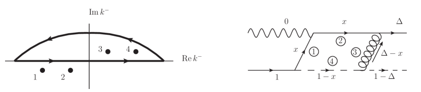
Figure 11: Illustration of the poles (left) and corresponding time-ordered diagram (right) of (44) for the kinematic regime Case A: $0<x<\Delta<1$. We choose to close the contour in the upper half-plane, enclosing the poles ③ and ④. Note that the placement of the poles is only schematic, indicating the sign of their imaginary part; the placement on the real axis has no significance.

For Case A: $0<x<\Delta<1$, we can close the contour in the upper half-plane, enclosing the poles ③ and ④, as in Fig. 11. Let us consider the possible contributions to (44) from the residue and imaginary parts of the various poles.

• Res[③] Im[②]: Kinematically Prohibited

This term would yield a contribution of

$$\mathcal{I} = \frac{-2\pi\,\mathrm{Im}\left\{\frac{1}{r^{-}+q^{-}-\frac{(\vec{k}_{\bot}-\vec{r}_{\bot})^{2}}{(\Delta-x)p^{+}}-\frac{(\vec{q}_{\bot}+\vec{k}_{\bot})^{2}}{xp^{+}}+i\epsilon}\right\}}{\left[r^{-}-\frac{(\vec{k}_{\bot}-\vec{r}_{\bot})^{2}}{(\Delta-x)p^{+}}-\frac{\vec{k}_{\bot}^{2}}{xp^{+}}\right]\left[r^{-}-p^{-}-\frac{(\vec{k}_{\bot}-\vec{r}_{\bot})^{2}}{(\Delta-x)p^{+}}+\frac{\vec{k}_{\bot}^{2}+\lambda^{2}}{(1-x)p^{+}}\right]}$$

$$= \frac{+2\pi^{2}\,\delta\left[r^{-}+q^{-}-\frac{(\vec{k}_{\bot}-\vec{r}_{\bot})^{2}}{(\Delta-x)p^{+}}-\frac{(\vec{q}_{\bot}+\vec{k}_{\bot})^{2}}{xp^{+}}\right]}{\left[r^{-}-\frac{(\vec{k}_{\bot}-\vec{r}_{\bot})^{2}}{(\Delta-x)p^{+}}-\frac{\vec{k}_{\bot}^{2}}{xp^{+}}\right]\left[r^{-}-p^{-}-\frac{(\vec{k}_{\bot}-\vec{r}_{\bot})^{2}}{(\Delta-x)p^{+}}+\frac{\vec{k}_{\bot}^{2}+\lambda^{2}}{(1-x)p^{+}}\right]}$$

$$\mathcal{I} = \frac{+2\pi^{2}\frac{x\Delta}{\Delta-x}p^{+}\,\delta\left[\left(\vec{q}_{\bot}+\frac{\Delta}{\Delta-x}\vec{k}_{\bot}-\frac{x}{\Delta-x}\vec{r}_{\bot}\right)^{2}\right]}{\left[r^{-}-\frac{(\vec{k}_{\bot}-\vec{r}_{\bot})^{2}}{(\Delta-x)p^{+}}-\frac{\vec{k}_{\bot}^{2}}{xp^{+}}\right]\left[r^{-}-p^{-}-\frac{(\vec{k}_{\bot}-\vec{r}_{\bot})^{2}}{(\Delta-x)p^{+}}+\frac{\vec{k}_{\bot}^{2}+\lambda^{2}}{(1-x)p^{+}}\right]},$$

but the argument of the delta function is positive definite, so it cannot be satisfied; this cut is kinematically prohibited because it corresponds to a 2 $\rightarrow$ 1 massless, on-shell process.

• Res[③] Im[①]: Proton Decay

Similarly, this cut would yield a contribution of

$$\mathcal{I} = \frac{+2\pi^{2}\,\delta\left[r^{-}-\frac{(\vec{k}_{\bot}-\vec{r}_{\bot})^{2}}{(\Delta-x)p^{+}}-\frac{\vec{k}_{\bot}^{2}}{xp^{+}}\right]}{\left[r^{-}+q^{-}-\frac{(\vec{k}_{\bot}-\vec{r}_{\bot})^{2}}{(\Delta-x)p^{+}}-\frac{(\vec{q}_{\bot}+\vec{k}_{\bot})^{2}}{xp^{+}}\right]\left[r^{-}-p^{-}-\frac{(\vec{k}_{\bot}-\vec{r}_{\bot})^{2}}{(\Delta-x)p^{+}}+\frac{\vec{k}_{\bot}^{2}+\lambda^{2}}{(1-x)p^{+}}\right]}$$ (A2)

$$\mathcal{I} \propto \delta\bigg{[}-x(\Delta-x)\left(\lambda^{2}-(1-\Delta)M^{2}\right)-x(\Delta-x)\vec{r}_{\bot}^{2}-x(1-\Delta)(\vec{k}_{\bot}-\vec{r}_{\bot})^{2}$$

$$- (1-\Delta)(\Delta-x)\vec{k}_{\bot}^{2}\bigg{]}.$$

All of the terms inside the delta-function are negative definite except for the first one, so we can impose the stability of the proton by requiring that

$$\lambda^{2}-(1-\Delta)M^{2}>0.$$ (A3)

• Res[③] Im[④] + Res[④] Im[③]: Kinematically Prohibited (Cancels)

The term corresponding to Res[③] Im[④] is

$$\mathcal{I}_{1} = \frac{-2\pi\,\mathrm{Im}\left\{\frac{1}{r^{-}-p^{-}-\frac{(\vec{k}_{\bot}-\vec{r}_{\bot})^{2}-i\epsilon}{(\Delta-x)p^{+}}+\frac{\vec{k}_{\bot}^{2}+\lambda^{2}-i\epsilon}{(1-x)p^{+}}}\right\}}{\left[r^{-}-\frac{(\vec{k}_{\bot}-\vec{r})^{2}}{(\Delta-x)p^{+}}-\frac{\vec{k}_{\bot}^{2}}{xp^{+}}\right]\left[r^{-}+q^{-}-\frac{(\vec{k}_{\bot}-\vec{r}_{\bot})^{2}}{(\Delta-x)p^{+}}-\frac{(\vec{q}_{\bot}+\vec{k}_{\bot})^{2}}{xp^{+}}\right]}$$

$$= \frac{\mp 2\pi^{2}\,\delta\left[r^{-}-p^{-}-\frac{(\vec{k}_{\bot}-\vec{r}_{\bot})^{2}}{(\Delta-x)p^{+}}+\frac{\vec{k}_{\bot}^{2}+\lambda^{2}}{(1-x)p^{+}}\right]}{\left[r^{-}-\frac{(\vec{k}_{\bot}-\vec{r})^{2}}{(\Delta-x)p^{+}}-\frac{\vec{k}_{\bot}^{2}}{xp^{+}}\right]\left[r^{-}+q^{-}-\frac{(\vec{k}_{\bot}-\vec{r}_{\bot})^{2}}{(\Delta-x)p^{+}}-\frac{(\vec{q}_{\bot}+\vec{k}_{\bot})^{2}}{xp^{+}}\right]}.$$

The sign of the $i\epsilon$ argument of the imaginary part is ambiguous; this is typically a signature of a false pole. Whatever the sign of this term, it is exactly canceled by the Res[④] Im[③] term:

$$\mathcal{I}_{2} = \frac{-2\pi\,\mathrm{Im}\left\{\frac{1}{p^{-}-\frac{\vec{k}_{\bot}^{2}+\lambda^{2}-i\epsilon}{(1-x)p^{+}}-r^{-}+\frac{(\vec{k}_{\bot}-\vec{r}_{\bot})^{2}-i\epsilon}{(\Delta-x)p^{+}}}\right\}}{\left[p^{-}-\frac{\vec{k}_{\bot}^{2}+\lambda^{2}}{(1-x)p^{+}}-\frac{\vec{k}_{\bot}^{2}}{xp^{+}}\right]\left[p^{-}+q^{-}-\frac{\vec{k}_{\bot}^{2}+\lambda^{2}}{(1-x)p^{+}}-\frac{(\vec{q}_{\bot}+\vec{k}_{\bot})^{2}}{xp^{+}}\right]}$$

$$= \frac{\pm 2\pi^{2}\,\delta\left[p^{-}-\frac{\vec{k}_{\bot}^{2}+\lambda^{2}}{(1-x)p^{+}}-r^{-}+\frac{(\vec{k}_{\bot}-\vec{r}_{\bot})^{2}}{(\Delta-x)p^{+}}\right]}{\left[p^{-}-\frac{\vec{k}_{\bot}^{2}+\lambda^{2}}{(1-x)p^{+}}-\frac{\vec{k}_{\bot}^{2}}{xp^{+}}\right]\left[p^{-}+q^{-}-\frac{\vec{k}_{\bot}^{2}+\lambda^{2}}{(1-x)p^{+}}-\frac{(\vec{q}_{\bot}+\vec{k}_{\bot})^{2}}{xp^{+}}\right]}.$$

Thus this cut, which would correspond to a massless, on-shell $1\rightarrow 2$ process, is kinematically prohibited.

• Res[④] Im[①]: Proton Decay

This cut corresponds to proton decay through a different channel, yielding a contribution of

$$\mathcal{I} = \frac{+2\pi^{2}\,\delta\left[p^{-}-\frac{\vec{k}_{\bot}^{2}+\lambda^{2}}{(1-x)p^{+}}-\frac{\vec{k}_{\bot}^{2}}{xp^{+}}\right]}{\left[p^{-}+q^{-}-\frac{\vec{k}_{\bot}^{2}+\lambda^{2}}{(1-x)p^{+}}-\frac{(\vec{q}_{\bot}+\vec{k}_{\bot})^{2}}{xp^{+}}\right]\left[p^{-}-r^{-}-\frac{\vec{k}_{\bot}^{2}+\lambda^{2}}{(1-x)p^{+}}+\frac{(\vec{k}_{\bot}-\vec{r}_{\bot})^{2}}{(\Delta-x)p^{+}}\right]}$$ (A6)

$$\mathcal{I} \propto \delta\bigg{[}-x\left(\lambda^{2}-(1-x)M^{2}\right)-\vec{k}_{\bot}^{2}\bigg{]}.$$

To prevent proton decay through this channel, we need to impose the slightly different condition

$$\lambda^{2}-(1-x)M^{2}>0$$ (A7)

• Res[④] Im[②]: Legal Cut

This combination is the only legal cut of the four denominators that can be put on-shell simultaneously. This contribution is

$$\mathcal{I} = \frac{+2\pi^{2}\,\delta\left[p^{-}+q^{-}-\frac{\vec{k}_{\bot}^{2}+\lambda^{2}}{(1-x)p^{+}}-\frac{(\vec{q}_{\bot}+\vec{k}_{\bot})^{2}}{xp^{+}}\right]}{\left[p^{-}-\frac{\vec{k}_{\bot}^{2}+\lambda^{2}}{(1-x)p^{+}}-\frac{\vec{k}_{\bot}^{2}}{xp^{+}}\right]\left[p^{-}-r^{-}-\frac{\vec{k}_{\bot}^{2}+\lambda^{2}}{(1-x)p^{+}}+\frac{(\vec{k}_{\bot}-\vec{r}_{\bot})^{2}}{(\Delta-x)p^{+}}\right]}.$$ (A8)

Expanding the argument of the delta function and keeping terms of order $\mathcal{O}\left(\frac{\bot}{Q}\right)$ gives

$$\delta\left[p^{-}+q^{-}-\frac{\vec{k}_{\bot}^{2}+\lambda^{2}}{(1-x)p^{+}}-\frac{(\vec{q}_{\bot}+\vec{k}_{\bot})^{2}}{xp^{+}}\right]\approx\frac{\Delta^{2}p^{+}}{Q^{2}}\,\delta\left[x-\left(1+2\frac{\vec{q}_{\bot}\cdot(\vec{k}_{\bot}-\vec{r}_{\bot})}{Q^{2}}\right)\Delta\right].$$ (A9)

The delta function sets $x\approx\Delta$ to leading order, but the singularity of the delta function only falls within the kinematic region of Case A, $0<x<\Delta<1$ if

$$\vec{q}_{\bot}\cdot(\vec{k}_{\bot}-\vec{r}_{\bot})<0,$$

which is restricted to only half of the total phase space of the $d^{2}k$ integral. As we will see, Case B complements this integral with the other half of the phase space. With this caveat, we can write a final expression for the imaginary part as

$$\mathcal{I}=\frac{2\pi^{2}\Delta^{2}p^{+}}{Q^{2}}\frac{\delta\left[x-\left(1+2\frac{\vec{q}_{\bot}\cdot(\vec{k}_{\bot}-\vec{r}_{\bot})}{Q^{2}}\right)\Delta\right]}{\left[p^{-}-\frac{\vec{k}_{\bot}^{2}+\lambda^{2}}{(1-x)p^{+}}-\frac{\vec{k}_{\bot}^{2}}{xp^{+}}\right]\left[p^{-}-r^{-}-\frac{\vec{k}_{\bot}^{2}+\lambda^{2}}{(1-x)p^{+}}+\frac{(\vec{k}_{\bot}-\vec{r}_{\bot})^{2}}{(\Delta-x)p^{+}}\right]}.$$ (A10)

For Case B: $0<\Delta<x<1$, we can close the contour in the upper half-plane, enclosing only the pole ④, as in Fig. 12. Again, we will consider the various contributions to (44) from the residue and imaginary part of the various poles.

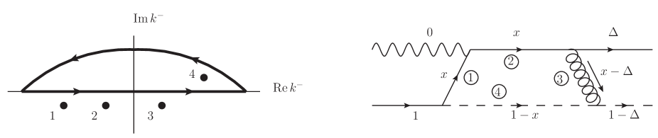
Figure 12: Illustration of the poles (left) and corresponding time-ordered diagram (right) of (44) for the kinematic regime Case B: $0<\Delta<x<1$. We choose to close the contour in the upper half-plane, enclosing only the pole ④. Note that the placement of the poles is only schematic, indicating the sign of their imaginary part; the placement on the real axis has no significance.

• Res[④] Im[①]: Proton Decay

This cut is exactly the same as the corresponding cut (A6) in Case A; it is unaffected by changing the sign of $(x-\Delta)$. Thus the condition to prohibit proton decay through this channel is the same: $\lambda^{2}-(1-x)M^{2}>0$.

• Res[④] Im[③]: Kinematically Prohibited

In this regime, it is explicitly impossible to perform this cut:

$$\mathcal{I} = \frac{+2\pi^{2}\,\delta\left[p^{-}-r^{-}-\frac{\vec{k}_{\bot}^{2}+\lambda^{2}}{(1-x)p^{+}}-\frac{(\vec{k}_{\bot}-\vec{r}_{\bot})^{2}}{(x-\Delta)p^{+}}\right]}{\left[p^{-}-\frac{\vec{k}_{\bot}^{2}+\lambda^{2}}{(1-x)p^{+}}-\frac{\vec{k}_{\bot}^{2}}{xp^{+}}\right]\left[p^{-}+q^{-}-\frac{\vec{k}_{\bot}^{2}+\lambda^{2}}{(1-x)p^{+}}-\frac{(\vec{q}_{\bot}+\vec{k}_{\bot})^{2}}{xp^{+}}\right]}$$ (A11)

$$\mathcal{I} \propto \delta\bigg{[}-(x-\Delta)^{2}\lambda^{2}-\left((1-x)\vec{r}_{\bot}+(1-\Delta)\vec{k}_{\bot}\right)^{2}\bigg{]}.$$

Since the argument is negative definite, this cut is kinematically prohibited.

• Res[④] Im[②]: Legal Cut

Again, this is the only combination of propagators that can be put on shell simultaneously. The expression is the same as in (A8) but with $x>\Delta$. This means that the delta function

$$\delta\left[x-\left(1+2\frac{\vec{q}_{\bot}\cdot(\vec{k}_{\bot}-\vec{r}_{\bot})}{Q^{2}}\right)\,\Delta\right]$$

has its singularity within the kinematic window of Case B, $0<\Delta<x<1$, if

$$\vec{q}_{\bot}\cdot(\vec{k}_{\bot}-\vec{r}_{\bot})>0.$$

Thus Case B gives rise to the same expression (A10) at leading order, but with validity in the complementary region of the $d^{2}k$ phase space; the final expression (A10) is thus valid for all $\vec{k}_{\bot}$.

The expression (A10) is illustrated in Fig. 4 in terms of the extra cut corresponding to putting the quark and the diquark propagators on mass shell.

Appendix B Integration in the DY Case

Here we want to evaluate the expression in (69). In Table 2 we classify the four poles ① - ④ of this expression as lying either above or below the $\mathrm{Re}\,k^{-}$ axis for the five distinct kinematic regimes: $(x<0<\Delta<\beta<1)$, $(0<x<\Delta<\beta<1)$, $(0<\Delta<x<\beta<1)$, $(0<\Delta<\beta<x<1)$, and $(0<\Delta<\beta<1<x)$. As before all the poles lie to one side of the real axis unless $0<x<1$, so there are three distinct cases to evaluate, each of which corresponds to a particular time-ordering of the diagram. We consider each of these cases below.

	Pole	$x<0$	$0<x<\Delta$	$\Delta<x<\beta$	$\beta<x<1$	$x>1$
①	$k^{-}=\frac{\vec{k}_{\bot}^{2}-i\epsilon}{xp^{+}}$	above	below	below	below	below
②	$k^{-}=q^{-}+\frac{(\vec{k}_{\bot}-\vec{q}_{\bot})^{2}-i\epsilon}{(x-\beta)p^{+}}$	above	above	above	below	below
③	$k^{-}=r^{-}+\frac{(\vec{k}_{\bot}-\vec{r}_{\bot})^{2}-i\epsilon}{(x-\Delta)p^{+}}$	above	above	below	below	below
④	$k^{-}=p^{-}-\frac{\vec{k}_{\bot}^{2}+\lambda^{2}-i\epsilon}{(1-x)p^{+}}$	above	above	above	above	below
	Contribution:	$0$	Case A	Case B	Case C	$0$

Table 2: Table classifying the pole locations of (69) as lying either above or below the $\mathrm{Re}\,k^{-}$ axis.

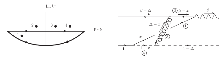
Figure 13: Illustration of the poles (left) and corresponding time-ordered diagram (right) of (69) for the kinematic regime Case A: $0<x<\Delta<\beta<1$. We choose to close the contour in the lower half-plane, enclosing only the pole ①. Note that the placement of the poles is only schematic, indicating the sign of their imaginary part; the placement on the real axis has no significance.

For Case A: $0<x<\Delta<\beta<1$, we choose to close the contour in the lower half-plane, enclosing only the pole ①, as shown in Fig. 13. Let us consider the possible contributions to (69) from the residue and imaginary parts of the various poles.

• Res[①] Im[④]: Proton Decay

This contribution would give

$$\mathcal{I} = \frac{+2\pi^{2}\delta\left[\frac{\vec{k}_{\bot}^{2}}{xp^{+}}-p^{-}+\frac{\vec{k}_{\bot}^{2}+\lambda^{2}}{(1-x)p^{+}}\right]}{\left[\frac{\vec{k}_{\bot}^{2}}{xp^{+}}-q^{-}+\frac{(\vec{k}_{\bot}-\vec{q}_{\bot})^{2}}{(\beta-x)p^{+}}\right]\left[\frac{\vec{k}_{\bot}^{2}}{xp^{+}}-r^{-}+\frac{(\vec{k}_{\bot}-\vec{r}_{\bot})^{2}}{(\Delta-x)p^{+}}\right]}$$

$$\propto \delta\left[x\left(\lambda^{2}-(1-x)M^{2}\right)+\vec{k}_{\bot}^{2}\right],$$

so we can prohibit proton decay through this channel by requiring that $\samepage{\lambda^{2}-(1-x)M^{2}>0}$.

• Res[①] Im[③]: Proton Decay

This contribution would give

$$\mathcal{I} = \frac{+2\pi^{2}\delta\left[\frac{\vec{k}_{\bot}^{2}}{xp^{+}}-r^{-}+\frac{(\vec{k}_{\bot}-\vec{r}_{\bot})^{2}}{(\Delta-x)p^{+}}\right]}{\left[\frac{\vec{k}_{\bot}^{2}}{xp^{+}}-q^{-}+\frac{(\vec{k}_{\bot}-\vec{q}_{\bot})^{2}}{(\beta-x)p^{+}}\right]\left[\frac{\vec{k}_{\bot}^{2}}{xp^{+}}-p^{-}+\frac{\vec{k}_{\bot}^{2}+\lambda^{2}}{(1-x)p^{+}}\right]}$$

$$\propto \delta\bigg{[}x(\Delta-x)\left(\lambda^{2}-(1-\Delta)M^{2}\right)+(1-\Delta)(\Delta-x)\vec{k}_{\bot}^{2}+x(\Delta-x)\vec{r}_{\bot}^{2}+$$

$$+ x(1-\Delta)(\vec{k}_{\bot}-\vec{r}_{\bot})^{2}\bigg{]}.$$

All of the momenta are positive definite, so we can prohibit proton decay through this channel by requiring that $\samepage{\lambda^{2}-(1-\Delta)M^{2}>0}$.

• Res[①] Im[②]: Legal Cut

This corresponds to the only legal cut of the diagram as shown in Fig. 13; it is permitted because it corresponds to a $2\rightarrow 1$ process in which the two massless quarks become a single “massive” time-like photon with “mass” $Q$. Equivalently, we can recognize that the subsequent leptonic decay of the time-like virtual photon makes this cut correspond to a massless, on-shell $2\rightarrow 2$ scattering process, which is allowed. This cut makes a contribution of

$$\mathcal{I} = \frac{+2\pi^{2}\delta\left[\frac{\vec{k}_{\bot}^{2}}{xp^{+}}-q^{-}+\frac{(\vec{k}_{\bot}-\vec{q}_{\bot})^{2}}{(\beta-x)p^{+}}\right]}{\left[\frac{\vec{k}_{\bot}^{2}}{xp^{+}}-r^{-}+\frac{(\vec{k}_{\bot}-\vec{r}_{\bot})^{2}}{(\Delta-x)p^{+}}\right]\left[\frac{\vec{k}_{\bot}^{2}}{xp^{+}}-p^{-}+\frac{\vec{k}_{\bot}^{2}+\lambda^{2}}{(1-x)p^{+}}\right]},$$ (B3)

and

$$\delta\left[\frac{\vec{k}_{\bot}^{2}}{xp^{+}}-q^{-}+\frac{(\vec{k}_{\bot}-\vec{q}_{\bot})^{2}}{(\beta-x)p^{+}}\right]\approx\frac{\Delta(\beta-\Delta)p^{+}}{Q^{2}}\ \delta\left[x-\left(1+2\,\frac{\vec{q}_{\bot}\cdot(\vec{k}_{\bot}-\vec{r}_{\bot})}{Q^{2}}\right)\Delta\right].$$

As usual, the $\delta$-function sets $x\approx\Delta$, but the singularity only falls within the kinematic window of Case A $(x<\Delta)$ for $\vec{q}_{\bot}\cdot(\vec{k}_{\bot}-\vec{r}_{\bot})<0$. As with DIS, this half of the $d^{2}k$ phase space will be complemented by an equal contribution for Case B $\Delta<x<\beta$. Thus, the legal cut gives

$$\mathcal{I}=\frac{2\pi^{2}\Delta(\beta-\Delta)p^{+}}{Q^{2}}\frac{\delta\left[x-\left(1+2\,\frac{\vec{q}_{\bot}\cdot(\vec{k}_{\bot}-\vec{r}_{\bot})}{Q^{2}}\right)\Delta\right]}{\left[\frac{\vec{k}_{\bot}^{2}}{xp^{+}}-r^{-}+\frac{(\vec{k}_{\bot}-\vec{r}_{\bot})^{2}}{(\Delta-x)p^{+}}\right]\left[\frac{\vec{k}_{\bot}^{2}}{xp^{+}}-p^{-}+\frac{\vec{k}_{\bot}^{2}+\lambda^{2}}{(1-x)p^{+}}\right]}$$ (B4)

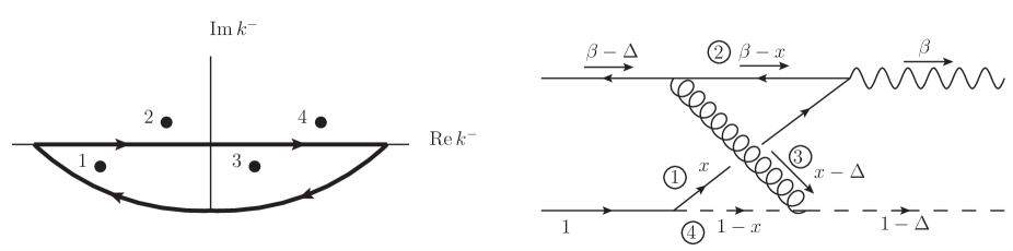
Figure 14: Illustration of the poles (left) and corresponding time-ordered diagram (right) of (69) for the kinematic regime Case B: $0<\Delta<x<\beta<1$. We choose to close the contour in the lower half-plane, enclosing the poles ① and ③. Note that the placement of the poles is only schematic, indicating the sign of their imaginary part; the placement on the real axis has no significance.

For Case B: $0<\Delta<x<\beta<1$, we close the contour in the lower half-plane, enclosing the poles ① and ③, as shown in Fig. 14. Let us consider the possible contributions to (69) from the residue and imaginary parts of the various poles.

• Res[①] Im[④]: Proton Decay

The evaluation of this cut proceeds along exactly the same lines as in (B) of Case A; the proton stability condition is unaffected by changing the sign of $(\Delta-x)$.

• Res[①] Im[③] + Res[③] Im[①]: Proton Decay (Cancels)

Evaluating Res[①] Im[③] would give a contribution of

$$\mathcal{I}_{1} = \frac{+2\pi\,\mathrm{Im}\left\{\frac{1}{\frac{\vec{k}_{\bot}^{2}-i\epsilon}{xp^{+}}-r^{-}-\frac{(\vec{k}_{\bot}-\vec{r}_{\bot})^{2}-i\epsilon}{(x-\Delta)p^{+}}}\right\}}{\left[\frac{\vec{k}_{\bot}^{2}}{xp^{+}}-q^{-}+\frac{(\vec{k}_{\bot}-\vec{q}_{\bot})^{2}}{(\beta-x)p^{+}}\right]\left[\frac{\vec{k}_{\bot}^{2}}{xp^{+}}-p^{-}+\frac{\vec{k}_{\bot}^{2}+\lambda^{2}}{(1-x)p^{+}}\right]}$$

$$= \frac{\pm 2\pi^{2}\delta\left[\frac{\vec{k}_{\bot}^{2}}{xp^{+}}-r^{-}-\frac{(\vec{k}_{\bot}-\vec{r}_{\bot})^{2}}{(x-\Delta)p^{+}}\right]}{\left[\frac{\vec{k}_{\bot}^{2}}{xp^{+}}-q^{-}+\frac{(\vec{k}_{\bot}-\vec{q}_{\bot})^{2}}{(\beta-x)p^{+}}\right]\left[\frac{\vec{k}_{\bot}^{2}}{xp^{+}}-p^{-}+\frac{\vec{k}_{\bot}^{2}+\lambda^{2}}{(1-x)p^{+}}\right]},$$

where the sign ambiguity of the $i\epsilon$ components indicates the presence of a false pole. Whatever the sign of (B), it is exactly canceled by the contribution of Res[③] Im[①]:

$$\mathcal{I}_{2} = \frac{+2\pi\,\mathrm{Im}\left\{\frac{1}{r^{-}+\frac{(\vec{k}_{\bot}-\vec{r}_{\bot})^{2}-i\epsilon}{(x-\Delta)p^{+}}-\frac{\vec{k}_{\bot}^{2}-i\epsilon}{xp^{+}}}\right\}}{\left[r^{-}-q^{-}+\frac{(\vec{k}_{\bot}-\vec{r}_{\bot})^{2}}{(x-\Delta)p^{+}}+\frac{(\vec{k}_{\bot}-\vec{q}_{\bot})^{2}}{(\beta-x)p^{+}}\right]\left[r^{-}-p^{-}+\frac{(\vec{k}_{\bot}-\vec{r}_{\bot})^{2}}{(x-\Delta)p^{+}}+\frac{\vec{k}_{\bot}^{2}+\lambda^{2}}{(1-x)p^{+}}\right]}$$

$$= \frac{\mp 2\pi^{2}\delta\left[r^{-}+\frac{(\vec{k}_{\bot}-\vec{r}_{\bot})^{2}}{(x-\Delta)p^{+}}-\frac{\vec{k}_{\bot}^{2}}{xp^{+}}\right]}{\left[r^{-}-q^{-}+\frac{(\vec{k}_{\bot}-\vec{r}_{\bot})^{2}}{(x-\Delta)p^{+}}+\frac{(\vec{k}_{\bot}-\vec{q}_{\bot})^{2}}{(\beta-x)p^{+}}\right]\left[r^{-}-p^{-}+\frac{(\vec{k}_{\bot}-\vec{r}_{\bot})^{2}}{(x-\Delta)p^{+}}+\frac{\vec{k}_{\bot}^{2}+\lambda^{2}}{(1-x)p^{+}}\right]}.$$

Thus $\mathcal{I}_{1}+\mathcal{I}_{2}=0$, so that proton decay by this channel is automatically prohibited for Case B.

• Res[③] Im[②]: Kinematically Prohibited

This contribution would be

$$\mathcal{I} = \frac{+2\pi^{2}\,\delta\left[r^{-}-q^{-}+\frac{(\vec{k}_{\bot}-\vec{r}_{\bot})^{2}}{(x-\Delta)p^{+}}+\frac{(\vec{k}_{\bot}-\vec{q}_{\bot})^{2}}{(\beta-x)p^{+}}\right]}{\left[r^{-}+\frac{(\vec{k}_{\bot}-\vec{r}_{\bot})^{2}}{(x-\Delta)p^{+}}-\frac{\vec{k}_{\bot}^{2}}{xp^{+}}\right]\left[r^{-}-p^{-}+\frac{(\vec{k}_{\bot}-\vec{r}_{\bot})^{2}}{(x-\Delta)p^{+}}+\frac{\vec{k}_{\bot}^{2}+\lambda^{2}}{(1-x)p^{+}}\right]}$$

$$\propto \delta\bigg{[}\left((x-\Delta)\vec{q}_{\bot}+(\beta-x)\vec{r}_{\bot}-(\beta-\Delta)\vec{k}_{\bot}\right)^{2}\bigg{]};$$

since the argument is positive definite, this cut is kinematically prohibited, as it corresponds to a $1\rightarrow 2$ massless process.

• Res[③] Im[④]: Kinematically Prohibited

This contribution would be

$$\mathcal{I} = \frac{+2\pi^{2}\,\delta\left[r^{-}-p^{-}+\frac{(\vec{k}_{\bot}-\vec{r}_{\bot})^{2}}{(x-\Delta)p^{+}}+\frac{\vec{k}_{\bot}^{2}+\lambda^{2}}{(1-x)p^{+}}\right]}{\left[r^{-}+\frac{(\vec{k}_{\bot}-\vec{r}_{\bot})^{2}}{(x-\Delta)p^{+}}-\frac{\vec{k}_{\bot}^{2}}{xp^{+}}\right]\left[r^{-}-q^{-}+\frac{(\vec{k}_{\bot}-\vec{r}_{\bot})^{2}}{(x-\Delta)p^{+}}+\frac{(\vec{k}_{\bot}-\vec{q}_{\bot})^{2}}{(\beta-x)p^{+}}\right]}$$

$$\propto \delta\bigg{[}(x-\Delta)^{2}\lambda^{2}+\left((1-x)\vec{r}_{\bot}-(1-\Delta)\vec{k}_{\bot}\right)^{2}\bigg{]};$$

since the argument is positive definite, this cut is kinematically prohibited.

• Res[①] Im[②]: Legal Cut

Again, this is the only legal cut of the diagram in Fig. 14. The expression is the same as in (B3) from Case A, but with $x>\Delta$. This means that the delta function

$$\delta\left[x-\left(1+2\,\frac{\vec{q}_{\bot}\cdot(\vec{k}_{\bot}-\vec{r}_{\bot})}{Q^{2}}\right)\Delta\right]$$

has its singularity within the kinematic window of Case B, $0<\Delta<x<\beta<1$, if $\vec{k}_{\bot}\cdot(\vec{q}_{\bot}-\vec{r}_{\bot})>0$. Hence we again recover (B4), but with validity in the other half of the $d^{2}k$ phase space. Cases A and B thus complement each other, and we will show that Case C does not make any contribution to (69).

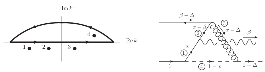
Figure 15: Illustration of the poles (left) and corresponding time-ordered diagram (right) of (69) for the kinematic regime Case C: $0<\Delta<\beta<x<1$. We choose to close the contour in the upper half-plane, enclosing only the pole ④. Note that the placement of the poles is only schematic, indicating the sign of their imaginary part; the placement on the real axis has no significance.

For Case C: $0<\Delta<\beta<x<1$, we choose to close the contour in the upper half plane, enclosing only the pole ④, as illustrated in Fig. 15. We demonstrate below that there is no viable cut for this time-ordering of the process.

• Res[④] Im[①]: Proton Decay

This cut is the same as in (B) of Case A; closing the contour in the other direction does not affect the overall sign of the contribution once the imaginary part is taken, and changing the signs of $\beta-x$ and $\Delta-x$ does not affect the proton stability condition.

• Res[④] Im[③]: Kinematically Prohibited

This cut is the same as in (B) of Case B; closing the contour in the other direction does not affect the overall sign, and changing the sign of $\beta-x$ does not affect the argument of the delta function. Hence this process is also kinematically forbidden.

• Res[④] Im[②]: Kinematically Prohibited

This is the only new cut that requires explicit calculation. This contribution would be

$$\mathcal{I} = \frac{+2\pi^{2}\,\delta\left[p^{-}-q^{-}-\frac{\vec{k}_{\bot}^{2}+\lambda^{2}}{(1-x)p^{+}}-\frac{(\vec{k}_{\bot}-\vec{q}_{\bot})^{2}}{(x-\beta)p^{+}}\right]}{\left[p^{-}-\frac{\vec{k}_{\bot}^{2}+\lambda^{2}}{(1-x)p^{+}}-\frac{\vec{k}_{\bot}^{2}}{xp^{+}}\right]\left[p^{-}-r^{-}-\frac{\vec{k}_{\bot}^{2}+\lambda^{2}}{(1-x)p^{+}}-\frac{(\vec{k}_{\bot}-\vec{r}_{\bot})^{2}}{(x-\Delta)p^{+}}\right]}$$

$$\propto \delta\bigg{[}-(\beta-\Delta)(x-\beta)(x-\Delta)\lambda^{2}-(1-x)(x-\beta)(1-\beta)\left(\vec{r}_{\bot}-\frac{1-\Delta}{1-\beta}\vec{q}_{\bot}\right)^{2}$$

$$- (1-\Delta)(\beta-\Delta)(1-\beta)\left(\vec{k}_{\bot}-\frac{1-x}{1-\beta}\vec{q}_{\bot}\right)^{2}\bigg{]}.$$

Since the argument is negative definite, this process is kinematically forbidden; this cut would not only correspond to proton decay in the lower half of the diagram in Fig. 15, but also a kinematically prohibited $3\rightarrow 1$ process in the upper half. Thus we have shown that there is no viable cut of the diagram for the kinematics of Case C, and this case makes no contribution to the asymmetry. Therefore (B4) gives the complete expression for the imaginary part and is our final result.

(B4) is illustrated in Fig. 6 in the text by the second (shorter) cut putting the quark and anti-quark propagators on mass shell.

References

- [1] S. M. Berman, J. D. Bjorken and J. B. Kogut, Phys. Rev. D 4, 3388 (1971).
- [2] Higher-twist contributions from direct subprocesses without quark fragmentation are discussed in F. Arleo, S. J. Brodsky, D. S. Hwang and A. M. Sickles, Phys. Rev. Lett. 105, 062002 (2010) [arXiv:0911.4604 [hep-ph]].
- [3] S. J. Brodsky, Nuovo Cim. C 035N2, 339 (2012) [arXiv:1112.0626 [hep-ph]].
- [4] S. J. Brodsky, D. S. Hwang and I. Schmidt, Phys. Lett. B 530, 99 (2002) [arXiv:hep-ph/0201296].
- [5] A. Metz, D. Pitonyak, A. Schafer, M. Schlegel, W. Vogelsang and J. Zhou, Phys. Rev. D 86, 094039 (2012) [arXiv:1209.3138 [hep-ph]].
- [6] D. W. Sivers, Phys. Rev. D 41, 83 (1990).
- [7] D. W. Sivers, Phys. Rev. D 43, 261 (1991).
- [8] J. C. Collins, Phys. Lett. B 536, 43 (2002) [arXiv:hep-ph/0204004].
- [9] S. J. Brodsky, D. S. Hwang and I. Schmidt, Nucl. Phys. B 642, 344 (2002) [arXiv:hep-ph/0206259].
- [10] Z. Lu and I. Schmidt, Phys. Rev. D 75, 073008 (2007) [arXiv:hep-ph/0611158].
- [11] A. Airapetian et al. [HERMES Collaboration], Phys. Rev. Lett. 94, 012002 (2005) [arXiv:hep-ex/0408013].
- [12] F. Bradamante [COMPASS Collaboration], Nuovo Cim. C 035N2, 107 (2012) [arXiv:1111.0869 [hep-ex]].
- [13] M. G. Alekseev et al. [COMPASS Collaboration], Phys. Lett. B 692, 240 (2010) [arXiv:1005.5609 [hep-ex]].
- [14] F. Bradamante, Mod. Phys. Lett. A 24, 3015 (2009).
- [15] C. Adolph et al. [COMPASS Collaboration], Phys. Lett. B 717, 383 (2012) [arXiv:1205.5122 [hep-ex]].
- [16] H. Avakian et al. [CLAS Collaboration], Phys. Rev. Lett. 105, 262002 (2010) [arXiv:1003.4549 [hep-ex]].
- [17] H. Gao et al., Eur. Phys. J. Plus 126, 2 (2011) [arXiv:1009.3803 [hep-ph]].
- [18] J. C. Collins, Nucl. Phys. B 396 (1993) 161 [hep-ph/9208213].
- [19] D. Boer and P. J. Mulders, Phys. Rev. D 57 (1998) 5780 [hep-ph/9711485].
- [20] M. Anselmino, D. Boer, U. D’Alesio and F. Murgia, Phys. Rev. D 63, 054029 (2001) [hep-ph/0008186].
- [21] G. Gustafson and J. Hakkinen, Phys. Lett. B 303, 350 (1993).
- [22] B. -Q. Ma, I. Schmidt, J. Soffer and J. -J. Yang, Phys. Lett. B 488, 254 (2000) [Phys. Lett. B 489, 293 (2000)] [hep-ph/0005210].
- [23] B. -Q. Ma, I. Schmidt, J. Soffer and J. -J. Yang, Eur. Phys. J. C 16, 657 (2000) [hep-ph/0001259].
- [24] M. Burkardt, Nucl. Phys. A 735, 185 (2004) [hep-ph/0302144].
- [25] S. J. Brodsky, B. Pasquini, B. W. Xiao and F. Yuan, Phys. Lett. B 687, 327 (2010) [arXiv:1001.1163 [hep-ph]].
- [26] J. Collins and J. W. Qiu, Phys. Rev. D 75, 114014 (2007) [arXiv:0705.2141 [hep-ph]].
- [27] D. Boer, S. J. Brodsky and D. S. Hwang, Phys. Rev. D 67, 054003 (2003) [arXiv:hep-ph/0211110].
- [28] S. Falciano et al. [NA10 Collaboration], Z. Phys. C 31, 513 (1986).
- [29] D. Boer, Phys. Rev. D 60, 014012 (1999) [arXiv:hep-ph/9902255].
- [30] C. S. Lam and W. -K. Tung, Phys. Rev. D 18, 2447 (1978).
- [31] C. S. Lam and W. -K. Tung,
- [32] Z. Lu and I. Schmidt, Phys. Rev. D 78, 034041 (2008)
- [33] S. J. Brodsky, P. Hoyer, N. Marchal, S. Peigne and F. Sannino, Phys. Rev. D 65, 114025 (2002) [arXiv:hep-ph/0104291].
- [34] C. Adloff et al. [H1 Collaboration], Z. Phys. C 76, 613 (1997) [arXiv:hep-ex/9708016].
- [35] J. Breitweg et al. [ZEUS Collaboration], Eur. Phys. J. C 6, 43 (1999) [arXiv:hep-ex/9807010].
- [36] A. V. Belitsky, X. Ji and F. Yuan, Nucl. Phys. B 656, 165 (2003) [arXiv:hep-ph/0208038].
- [37] D. Boer, P. J. Mulders and F. Pijlman, Nucl. Phys. B 667 (2003) 201 [hep-ph/0303034].
- [38] J. W. Qiu, private communications.
- [39] J. w. Qiu and G. F. Sterman, Phys. Rev. Lett. 67, 2264 (1991).
- [40] J. w. Qiu and G. F. Sterman, Phys. Rev. D 59, 014004 (1999) [arXiv:hep-ph/9806356].
- [41] A. H. Mueller and S. Munier, Nucl. Phys. A 893, 43 (2012) [arXiv:1206.1333 [hep-ph]].
- [42] G. P. Lepage and S. J. Brodsky, Phys. Rev. D 22, 2157 (1980).
- [43] S. J. Brodsky, H. C. Pauli and S. S. Pinsky, Phys. Rept. 301, 299 (1998) [arXiv:hep-ph/9705477].
- [44] Y. V. Kovchegov and M. D. Sievert, Phys. Rev. D 86, 034028 (2012) [Erratum-ibid. D 86, 079906 (2012)] [arXiv:1201.5890 [hep-ph]].
- [45] M. Burkardt and D. S. Hwang, Phys. Rev. D 69 (2004) 074032 [hep-ph/0309072].
- [46] R. E. Cutkosky, J. Math. Phys. 1, 429 (1960).
- [47] D. Boer, L. Gamberg, B. Musch and A. Prokudin, JHEP 1110, 021 (2011) [arXiv:1107.5294 [hep-ph]].