First-principle calculation of solar cell efficiency under incoherent illumination

Abstract

Because of the temporal incoherence of sunlight, solar cells efficiency should depend on the degree of coherence of the incident light. However, numerical computation methods, which are used to optimize these devices, fundamentally consider fully coherent light. Hereafter, we show that the incoherent efficiency of solar cells can be easily analytically calculated. The incoherent efficiency is simply derived from the coherent one thanks to a convolution product with a function characterizing the incoherent light. Our approach is neither heuristic nor empiric but is deduced from first-principle, i.e. Maxwell’s equations. Usually, in order to reproduce the incoherent behavior, statistical methods requiring a high number of numerical simulations are used. With our method, such approaches are not required. Our results are compared with those from previous works and good agreement is found.
^†These authors have contributed equally to this work.

I Introduction

Improvement of solar cell technology as well as cost reduction is an increasingly challenging topic in the quest of renewable energy sources. One of the strategy currently followed to reduce the fabrication cost is the use of ultrathin active layers. This approach could help reducing the cost of photovoltaic technologies since a smaller quantity of material is used Tsakalakos ; Nelson . However, reducing the thickness brings new problems. The fact that the film thickness could be much lower than the absorption length leads to a significant reduction of the absorption. Ultrathin technologies need solutions to keep solar light absorption high. One already well-known solution is the use of front-side or/and back-side surface texturing to help coupling incident light into the active layer via light trapping techniques Zeman ; Campbell ; Yablonovitch ; Deparis . The optimization of light-trapping structures (see Fig. 1(a)) in solar cell is still of high interest Gjessing ; Herman . In this approach, numerical computations are needed to investigate how electromagnetic field propagates in those devices. Usually, numerical methods used for calculating the absorption inside a solar cell (Finite-Difference Time-Domain method (FDTD) FDTD1 ; FDTD2 , Rigorous Coupled Wave Analysis (RCWA) Moharam ; code1 ; code2 ; code3 , …) basically consider the cell response under coherent incident light. Unfortunately, it is known that the absorption of an optical device depends on the coherent or incoherent nature of the light. Coherent light leads to oscillations (such as Fabry-Perot) in the absorption spectrum. Incoherent light instead, leads to the disappearance of these oscillations due to destructive-interference effects: a fact that is well known from anyone performing measurements in solar cells. Therefore, the calculated absorption spectrum of the active layer is strongly affected by the choice of the incident source (coherent or not). Since the absorption spectrum is used to determine the photocurrent and the efficiency of solar cells Herman ; Jin ; Zhao , it should be recommended to use only incoherent absorption spectrum. Solar light is indeed a strongly incoherent light source: incoming waves from the sun have a finite coherence time (finite spectral width). The photocurrent $J$ supplied by the solar cell is given by:

$$J=\frac{e}{hc}\int A(\lambda)S_{G}(\lambda)\lambda d\lambda$$ (1)

where $A(\lambda)$ is the absorption spectrum and $S_{G}(\lambda)$ the global power spectral density of the sun. In most studies, the absorption spectrum $A(\lambda)$ is computed from numerical codes which propagate the electromagnetic field. Nevertheless, such computed $A(\lambda)$ is calculated from coherent fields and then we write $A(\lambda)=A_{coh}(\lambda)$. This quantity does not correspond to the required effective incoherent absorption $A_{incoh}(\lambda)$ experienced by the solar cell. In order to theoretically predict the performance of a solar cell, it is therefore very important to improve numerical methods and to take incoherent incident light into account, i.e. to use $A(\lambda)=A_{incoh}(\lambda)$ in Eq. (1).

It must be noted that, as far as the propagation of the electric field of incident optical radiation is concerned, a solar cell, whatever the complexity of its structure is, behaves as a linear system (thanks to Maxwell equations), which is fully characterized by its scattering matrix (see Appendix A). However, as soon as energy fluxes need to be calculated, linearity does not stand anymore since the intensity (Poynting vector flux) is proportional to the electric field squared, i.e. $I\propto E\cdot E^{*}=|E|^{2}$. The way the square modulus of the fields enters into the calculation of the absorption (reflectance, transmittance) of the system is far from being trivial (see, for example, the case of RCWA method, in Appendix B). In any case, there exists no transfer function relating linearly the solar cell absorption to the incident Poynting vector flux. The fact that the relevant quantities (absorbed flux, photocurrent,…) do not obey the superposition principle (since $I\propto|E|^{2}$) prevents us from applying common principles of the linear response theory random_signal . In particular, the incoherent response cannot be treated in the same way as the coherent one, a fact that is known for long time in optics BornWolf , at least for simple cases, such as thin films.

In order to overcome this limitation, numerical solutions have been proposed for modeling incoherent processes Prentice_2000 ; Mitsas ; Troparevsky ; Niv ; Katsidis ; Prentice_99 ; Centurioni ; Lee ; Santbergen . Basically, light propagation is computed many times for various incident waves, and the final result relies on a global numerical statistical analysis. Many recipes and algorithms have been proposed to achieve this task. Nevertheless, in the present article, we show that it is not necessary to upgrade numerical codes or to perform time consuming statistical analysis in order to deal with incoherent light. Indeed, the efficiency of solar cells under incoherent light illumination can be analytically calculated from the coherent response computed with usual numerical codes, as explained hereafter. Results obtained with our method are compared with those from previous studies.

II Incoherent absorption

 

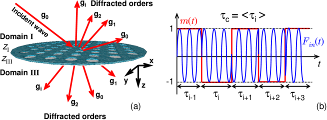
Figure 1: (a) Sketch of a light trapping diffracting structure ($Z_{I}<z<Z_{III}$) with many diffraction orders. Domains $I$ and $III$ are respectively the incident and emergence media. (b) Model of field amplitude $F_{in}(t)$ for the incoherent monochromatic incident light. $m(t)$ is the corresponding modulation which characterizes the random phase switching at different times $\tau_{i}$. $\tau_{c}$ is the coherence time, equal to the average value $<\tau_{i}>$.

When the active domain of a solar cell is illuminated by a coherent monochromatic light, a steady state is reached in which the intensity of the electromagnetic field $\left|\mathbf{E}(\omega,\mathbf{r})\right|^{2}$ exhibits a typical stationary pattern. The absorption coefficient $A_{coh}(\omega)$ is then given by BornWolf :

$$A_{coh}(\omega)=-\frac{\varepsilon_{0}\omega}{2P_{in}}\int_{V}\varepsilon^{\prime\prime}(\omega,\mathbf{r})\left|\mathbf{E}(\omega,\mathbf{r})\right|^{2}d^{3}r$$ (2)

where $\varepsilon^{\prime\prime}(\omega,\mathbf{r})$ is the imaginary part of the permittivity of the active medium of the solar cell and $P_{in}$ is the power of the incident light. $V$ is the volume of the active domain. By contrast, if the light is incoherent, the incident electromagnetic field exhibits a time-dependent fluctuating behaviour with a characteristic time $\tau_{c}$, defined as the coherence time of the incident light. Therefore, light inside the active volume cannot exhibit the same constructive interference pattern as in the fully coherent case: incoherence affects the way the light propagates. In addition, a specific medium mainly interacts with light through electronic and ionic motions of its components. As a consequence, the response of a medium to an incident electromagnetic wave is not instantaneous and occurs with a given response time $T$ related to dielectric relaxation time and/or to charge carrier generation and recombination. If $\tau_{c}\ll T$, then the medium undergoes many different field intensity patterns during the characteristic time $T$. As a result, the absorption and the generated photocurrent both fluctuate in time. The effective incoherent absorption $A_{incoh}(\omega)$ (and the photocurrent) is the time averaged value during a typical time about $T$ (see appendix A).

It is important to point out that the incoherent absorption $A_{incoh}(\omega)$ is physically different from the coherent one $A_{coh}(\omega).$ Indeed, $A_{coh}(\omega)$ can be considered as an intrinsic property of the solar cell which only depends on its geometry and on its constitutive materials. By contrast, $A_{incoh}(\omega)$ reflects the effective measured response of the solar cell while it interacts with its environment, i.e. for instance when the photocurrent is produced and flows in a closed electrical circuit.

In a numerical computation approach, the absorption coefficient $A$ can be obtained from at least two ways. In FDTD for instance, Eq. (2) can be used as such, since maps of the electromagnetic field are directly computed. In RCWA, reflection $R$ and transmission $T$ are calculated and $A$ is deduced from $A=1-R-T$. In the following, we consider a RCWA formalism of the light propagation (see appendix B), and we use it to determine the effective incoherent absorption $A_{incoh}(\omega)$ (see Appendix A). The main results of Appendix A are summarized hereafter.

Let us consider an incoherent radiation spectrum, the solar spectrum for instance. Such a spectrum can be considered as constituted by an infinite set of incoherent quasi-monochromatic spectral lines, each line being expressed by the temporal signal:

$$\left|F_{in}(t)\right\rangle=m(t)e^{-i\omega_{c}t}\left|F_{in}^{(0)}\right\rangle.$$ (3)

The bracket notation denotes the fact that $\left|F_{in}(t)\right\rangle$ is a supervector which contains the time-dependent complex Fourier components related to each diffraction orders (see Appendix B). $\left|F_{in}^{(0)}\right\rangle$ describes the incident wave amplitudes, assumed to be non zero only for the zeroth diffraction order (see Fig. 1(a) and Appendix B). $\omega_{c}$ is the angular frequency. The function $m(t)$ is a modulation which ensures the incoherent behaviour of the spectral line. $m(t)$ is a stochastic function which has an average time fluctuation equal to the coherence time $\tau_{c}$. As an illustration, a simple but non-restrictive modulation is shown in Fig. 1(b). The autocorrelation function of a random process has a spectral representation given by the power spectrum of that process (Wiener Kinchine’s theorem) random_signal . The function $m(t)$ can therefore be characterized by its spectral density:

$$D(\omega)=\left|m(\omega)\right|^{2}$$ (4)

with $m(\omega)=\int m(t)e^{i\omega t}dt$. We then introduce the normalized incoherence function $I(\omega)$,

$$I(\omega)=\frac{D(\omega)}{\int D(\omega)d\omega}$$ (5)

which characterizes the incoherence of incident light. Assuming that $m(t)$ describes a random process which follows a Gaussian distribution, the incoherent source illuminating the device is characterized by a Gaussian spectral density $D(\omega)$. As a result, the incoherence function is simply written as:

$$I(\omega)=\tau_{c}\sqrt{\frac{\ln 2}{\pi^{3}}}e^{-\frac{\ln 2}{\pi^{2}}\tau_{c}^{2}\omega^{2}}$$ (6)

with a Full Width at Half Maximum $\Delta\omega=2\pi/\tau_{c}$. Though the coherence time is estimated from the solar spectrum, it must be noted that $D(\omega)$ is not a model of the solar spectrum. $D(\omega)$ simply describes the stochastic behaviour of each spectral line composing the whole solar spectrum itself.

It can then be shown (see Appendix A) that the incoherent absorption $A_{incoh}(\omega)$ results from the convolution product, noted $\star$, between the coherent absorption $A_{coh}(\omega)$ and the incoherence function $I(\omega)$:

$$A_{incoh}(\omega)=I(\omega)\star A_{coh}(\omega).$$ (7)

This extremely simple formula is easy to use in practice. But its demonstration is not obvious and is therefore detailed in Appendix A. Eq. (7) can also be used to compute incoherent reflection and transmission spectra from their coherent counterparts (see appendix A).

III Numerical Application

 

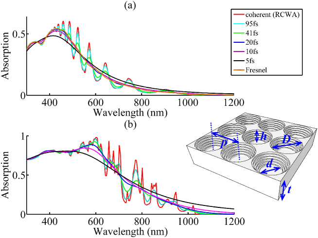
Figure 2: Simulation of the absorption spectra of planar and corrugated $500$ nm-thick c-Si slabs. The coherent spectra were obtained using RCWA and the incoherent ones using our convolution formula, Eq. (7). (a) Absorption spectra of the planar slab according to various coherence times. (b) Absorption spectra of the corrugated slab according to various coherence times. Inset: corrugated structure ; $p=500$ nm, $t=500$ nm, $h=300$ nm, $D=450$ nm, $d=320$ nm. The structure follows a super-Gaussian profile with $m=3$ (see Ref. Herman ).

In order to illustrate the usefulness of the convolution formula, i.e. Eq. (7), we use it for the calculation of the incoherent absorption of a $500$ nm-thick crystalline silicon (c-Si) slab either planar (see Fig. 2(a)) or corrugated (see Fig. 2(b)).

The first step is the numerical calculation of the coherent absorption using the RCWA method (see Fig. 2, red lines). In the RCWA simulations, we use unpolarized light at normal incidence, where the $(x,z)$ plane is the plane of incidence (polar and azimuthal angles equal to $0$) (see Fig. 1(a)). The permittivities of materials are taken from the literature Palik . The second step is the convolution of the coherent absorption spectrum with the incoherence function $I(\omega)$. This step leads to the incoherent absorption spectra.

 

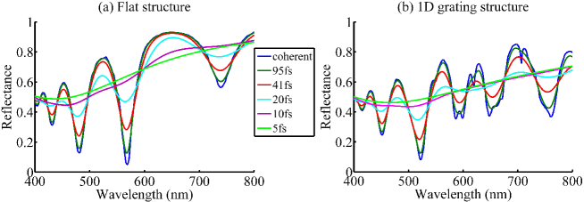
Figure 3: Comparison between the coherent spectra obtained with the RCWA method (blue lines) and incoherent spectra with various coherence times, for planar and grating structures, defined in Lee . (a) Reflectance spectrum of an unpatterned c-Si layer ($225$ nm) deposited on a $75$ nm-thick Au film on a glass substrate. (b) Reflectance spectrum of the whole grating structure.

The first step is the longest one. For example, using $225$ orders of diffraction ($15$ plane waves along the $x$ direction and $15$ plane waves along the $y$ direction), it takes a few hours. The second step is very fast. It takes only a few minutes on a personal computer. It is an important improvement in terms of computational time, in comparison with other computational methods Prentice_2000 ; Mitsas ; Troparevsky ; Niv ; Katsidis ; Prentice_99 ; Centurioni ; Lee ; Santbergen . In these methods, the first step is performed several times for various incident waves, and the final result relies on a global numerical statistical analysis. Five different coherence times are considered here ($95$ fs, $41$ fs, $20$ fs, $10$ fs and $5$ fs). These values are chosen according to the ones used by W. Lee and coworkers in a previous work Lee .

In the case of a planar slab, computed spectra are compared with the approximate incoherent absorption spectrum obtained from a standard analytical expression of the absorption using Fresnel equations BornWolf , but in which propagation phases are roughly set to zero to mimic incoherence (orange curve in Fig. 2(a)). We note that this kind of analytical expression must be considered carefully in the present case. Indeed, such an expression considers the effect of incoherence on light propagation only and does not consider the incoherent response of the permittivities of the materials, contrary to our present approach using convolution (see appendix A). In spite of that, both spectra (orange and black curves in Fig. 2(a)) are quite similar, which validates our method (in our method, the incoherence limit is approached by taking $\tau_{c}=5$ fs). The weak discrepancies are due to the absence of incoherent permittivity response in the Fresnel approach.

We also reproduced some results reported in the literature Lee . Two structures were studied under TM polarization. The first one is a $225$ nm-thick film of crystalline silicon (c-Si), deposited on a $75$ nm-thick layer of Gold (Au) on a glass substrate. The second one is a $250$ nm-thick c-Si film deposited on a gold grating on a glass substrate. The gold grating has a height of $50$ nm, a period of $400$ nm and a fill factor of $0.5$. The grating is built on a $50$ nm-thick gold layer. A sketch of both structures can be found in Lee . The results obtained with the convolution formula are presented in Fig. 3 and can be compared with those shown in figures 2 and 4 in Lee . Some small discrepancies are observed, which are due to the fact that we did not use the same numerical method (RCWA vs FDTD). However, our results give the same trends as the results obtained by W. Lee et al. It is therefore possible to account for the light incoherence with a simple method, which does not require long computational times contrary to other previously reported methods.

Coming back to Fig. 2, the absorption spectra of a three-dimensional corrugated $500$ nm-thick c-Si slab were calculated using the same method as for the planar slab. The corrugation follows a super-Gaussian profile such as the one defined in Herman ($m=3$). The period of the corrugation is $500$ nm and its height is $300$ nm. The absorption spectra according to various coherence times are shown in Fig. 2(b). We notice that the value of the coherence time affects the absorption spectrum. The highest coherence time (here $95$ fs) leads to the strongest oscillations in the spectrum. Physically, these oscillations are due to Fabry-Perot resonances (in the thin-slab) and to guided mode resonances (enabled by the corrugation). With the decrease of $\tau_{c}$, these oscillations are expected to be smoothened which is actually observed when $\tau_{c}<20$ fs. This smoothing effect is indeed observed when measuring absorption spectra with an incoherent source.

We finally calculated the photocurent of the corrugated slab, according to Eq. (1) (see Table 1). The aim was to quantify the effect of the coherence time on the value of the photocurrent. The photocurrent fluctuates as the coherence time varies. As expected, the incoherent light behaviour affects both the absorption spectrum and the photocurrent.

$\tau_{c}(fs)$	$j_{sc}(mA/cm^{2})$
coherent	20.69
95	20.70
41	20.75
20	20.81
10	20.93
5	21.16
3	21.14
2.5	21.01

Table 1: Computed photocurrents related to the corrugated device of Fig. 2(b) for various coherence times. Photocurrent was integrated over the spectral range: 300 nm - 1200 nm.

IV Conclusion

We demonstrated that reflection, transmission, and absorption spectra of a photonic structure illuminated with incoherent light can be easily calculated. The only input is the knowledge of their coherent counterparts and of the coherence time of the source (used to determine the incoherence function). The incoherent response is simply the convolution between a function accounting for the incoherent source and the coherent response. This result is theoretically demonstrated from first principle and is confirmed by numerical simulations. In analogy with signal processing theory, it can be interpreted as the consequence, in the frequency domain, of the temporal filtering associated with the intrinsic incoherent modulation. The proposed method allows to significantly simplify the description of incoherent phenomena which are regarded as key problem in solar cells optimization. The inherent simplicity of our method allows to minimize the computational time cost and the algorithm complexity. Reflection, transmission, and absorption spectra, but also the photocurrent, were shown to depend on the coherence time.

Appendix A Appendix: Demonstration of the convolution formula

A.1 Scattering matrix as response function

The following demonstration is based on the formalism of the Rigorous Coupling Wave Analysis (RCWA) Moharam ; code1 ; code2 ; code3 . This analysis takes into account the periodicity of the device and describes the permittivity ($\epsilon$) through Fourier series. The electromagnetic field is then described by Bloch waves also expanded in Fourier series. In this formalism, the Maxwell’s equations take the form of a matricial first-order differential equation in the $z$ variable. The $z$ axis is perpendicular to the plane ($x$,$y$) where the permittivity is periodic (Fig. 1(a)). The essence of the method is to solve this equation but is not the topic of the present article.

Reflected and transmitted field amplitudes are linked to the incident field amplitudes by the use of the scattering matrix ($S$) which is calculated by solving Maxwell equations using Fourier series (see Appendix B). Let us define $F_{scat}$ as the scattered field and $F_{in}$ as the incident field, such that the associated supervectors are:

$$\left|F_{scat}\right\rangle=\left[\begin{array}[]{c}\overline{N}_{III}^{+}\\ \overline{X}_{III}^{+}\\ \overline{N}_{I}^{-}\\ \overline{X}_{I}^{-}\end{array}\right],\left|F_{in}\right\rangle=\left[\begin{array}[]{c}\overline{N}_{I}^{+}\\ \overline{X}_{I}^{+}\\ \overline{N}_{III}^{-}\\ \overline{X}_{III}^{-}\end{array}\right].$$ (A.1)

The subscripts $I$ and$\ III$ denote the incidence and emergence media, respectively. The superscripts $+$ and $-$ denote the positive and negative directions along the $z$ axis associated with the field propagation. All the Fourier components related to the reciprocal vectors $\mathbf{g}$ are contained in the vector $\overline{N}$ or $\overline{X}$ . For each vector $\mathbf{g}$ of the reciprocal lattice, $N_{I,\mathbf{g}}^{-}$ and $X_{I,\mathbf{g}}^{-}$ are the $s$ and $p$ polarization amplitudes of the reflected field, respectively. $N_{III,\mathbf{g}}^{+}$ and $X_{III,\mathbf{g}}^{+}$ represent the $s$ and $p$ polarization amplitudes of the transmitted field. Accordingly, $N_{I,\mathbf{0}}^{+}$ and $X_{I,\mathbf{0}}^{+}$ define the $s$ and $p$ polarization amplitudes of the incident field, respectively. $F_{scat}$ is connected to $F_{in}$ via the scattering matrix by:

$$S(\omega)\left|F_{in}(\omega)\right\rangle=\left|F_{scat}(\omega)\right\rangle.$$ (A.2)

The flux $J$ of the Poynting vector through a unit cell area $\sigma$ for the incident plane wave in homogeneous medium $I$ is given by:

$$J_{in}=\sigma\frac{1}{2}\varepsilon_{0}c\sqrt{\varepsilon_{I}}\cos\theta\left\langle F_{in}(\omega)\right|\left.F_{in}(\omega)\right\rangle.$$ (A.3)

For the refracted ($X=R$) or transmitted ($X=T$) wave, it is given by

$$J_{X}=\left\langle F_{scat}(\omega)\right|C_{X}^{\dagger}(\omega)C_{X}(\omega)\left|F_{scat}(\omega)\right\rangle,$$ (A.4)

where we define the connection matrices

$$C_{T}(\omega)=\left[\begin{array}[]{cccc}Q_{III}(\omega)&0&0&0\\ 0&Q_{III}(\omega)&0&0\\ 0&0&0&0\\ 0&0&0&0\end{array}\right],C_{R}(\omega)=\left[\begin{array}[]{cccc}0&0&0&0\\ 0&0&0&0\\ 0&0&Q_{I}(\omega)&0\\ 0&0&0&Q_{I}(\omega)\end{array}\right],$$ (A.5)

with

$$Q_{I(III)}(\omega)=\left[\begin{array}[]{ccc}...&0&0\\ 0&\sqrt{\frac{\sigma}{2\mu_{0}\omega}Re\left\{k_{I(III),\mathbf{g},z}\right\}}&0\\ 0&0&...\end{array}\right].$$ (A.6)

In (A.6), $k_{u,\mathbf{g},z}=[(\varepsilon_{u}(\frac{\omega}{c})^{2}-|\mathbf{k}_{//}+\mathbf{g}|^{2})]^{1/2}$ with $\mathbf{k}_{//}$ and $\omega$ being the wave vector component parallel to the surface and the pulsation of the incident plane wave, respectively. $\varepsilon_{u}$ represents either the permittivity of the incident medium ($\varepsilon_{I}$), or of the emergence medium ($\varepsilon_{III}$). We now introduce a convenient notation:

$$J_{X}=\left\langle F_{X}(\omega)\right|\left.F_{X}(\omega)\right\rangle,$$ (A.7)

where

$$\left|F_{X}(\omega)\right\rangle=S_{X}(\omega)\left|F_{in}(\omega)\right\rangle,$$ (A.8)

with

$$S_{X}(\omega)=C_{X}(\omega)S(\omega).$$ (A.9)

A.2 R, T, A coefficients for a coherent monochromatic incident wave

Let us first consider a coherent monochromatic incident wave:

$$\left|F_{in}(t)\right\rangle=\left|F_{in}^{(0)}\right\rangle e^{-i\omega_{c}t}$$ (A.10)

with an (optical) angular frequency $\omega_{c}$. The response $\left|F_{X}(t)\right\rangle$ of the device is given by random_signal

$$\left|F_{X}(t)\right\rangle=S_{X}(t)\star\left|F_{in}(t)\right\rangle$$ (A.11)

where $\star$ denotes the convolution product. The response can then be written explicitely as:

$$\left|F_{X}(t)\right\rangle = \int S_{X}(t-t^{\prime})e^{-i\omega_{c}t^{\prime}}dt^{\prime}\left|F_{in}^{(0)}\right\rangle$$ (A.12)

$$= e^{-i\omega_{c}t}S_{X}(\omega_{c})\left|F_{in}^{(0)}\right\rangle,$$

where

$$S_{X}(\omega_{c})=\int S_{X}(t^{\prime})e^{i\omega_{c}t^{\prime}}dt^{\prime}$$ (A.13)

is the Fourier transform of $S_{X}$ scattering matrix defined in (A.9). We note that $S_{X}(-\omega_{c})=S_{X}^{*}(\omega_{c})$ since $S_{X}(t)$ must be real.

From (A.12), we set

$$\left|F_{X}(t)\right\rangle=\left|F_{X}^{(0)}\right\rangle e^{-i\omega_{c}t},$$ (A.14)

with

$$\left|F_{X}^{(0)}\right\rangle=S_{X}(\omega_{c})\left|F_{in}^{(0)}\right\rangle.$$ (A.15)

We remind here that $X$ stands either for the reflected ($R$) or the transmitted ($T$) wave. Reflection $R_{coh}$ and transmission $T_{coh}$ coefficients associated with a coherent process can be obtained thanks to:

$$R_{coh}(\omega_{c})=\frac{J_{R}}{J_{in}}=\frac{\left\langle F_{R}^{(0)}\right|\left.F_{R}^{(0)}\right\rangle}{J_{in}}=\frac{\left\langle F_{in}^{(0)}\right|S_{R}^{\dagger}(\omega_{c})S_{R}(\omega_{c})\left|F_{in}^{(0)}\right\rangle}{J_{in}},$$ (A.16)

and

$$T_{coh}(\omega_{c})=\frac{J_{T}}{J_{in}}=\frac{\left\langle F_{T}^{(0)}\right|\left.F_{T}^{(0)}\right\rangle}{J_{in}}=\frac{\left\langle F_{in}^{(0)}\right|S_{T}^{\dagger}(\omega_{c})S_{T}(\omega_{c})\left|F_{in}^{(0)}\right\rangle}{J_{in}}.$$ (A.17)

The absorption $A_{coh}$ is then simply given by the energy conservation law: i.e. $A_{coh}=1-R_{coh}-T_{coh}$. The incident Ponyting flux $J_{in}(t)$, i.e.

$$J_{in}(t) = \sigma\frac{1}{2}\varepsilon_{0}c\sqrt{\varepsilon_{I}}\cos\theta\left\langle F_{in}(t)\right|\left.F_{in}(t)\right\rangle$$ (A.18)

$$= \sigma\frac{1}{2}\varepsilon_{0}c\sqrt{\varepsilon_{I}}\cos\theta\left\langle F_{in}^{(0)}\right|\left.F_{in}^{(0)}\right\rangle,$$

turns out to be time independent (see Eq. (B.13) in Appendix B). Therefore, the time-averaged incident flux $J_{in}$ is identical to $J_{in}(t)$

$$J_{in}=\frac{1}{T}\int_{-T/2}^{T/2}J_{in}(t)dt=\sigma\frac{1}{2}\varepsilon_{0}c\sqrt{\varepsilon_{I}}\cos\theta\left\langle F_{in}^{(0)}\right|\left.F_{in}^{(0)}\right\rangle\equiv J_{in}(t).$$ (A.19)

This result is only valid as far as the incident wave is coherent.

A.3 R, T, A coefficients for an incoherent monochromatic incident wave

Let us now consider an incoherent quasi-monochromatic incident wave:

$$\left|F_{in}(t)\right\rangle=\left|F_{in}^{(0)}\right\rangle m(t)e^{-i\omega_{c}t}.$$ (A.20)

By quasi monochromatic, we mean that the spectral line has a finite though narrow spectral width. As explained in the present article, the function $m(t)$ is a modulation which ensures the incoherent behaviour. On average, $m(t)$ has a coherence time equal to $\tau_{c}$ (see Fig. 1(b)). Thanks to the Wiener-Khinchine theorem, the autocorrelation function of a random process has a spectral decomposition given by the power spectrum of that processrandom_signal . The function $m(t)$ is then equally characterized by its spectral density:

$$D(\omega)=\left|m(\omega)\right|^{2},$$ (A.21)

where

$$m(\omega)=\int m(t)e^{i\omega t}dt$$ (A.22)

is the Fourier transform of $m(t)$.

The device response is then calculated by the same convolution product as in (A.11):

$$\left|F_{X}(t)\right\rangle = S_{X}(t)\star\left|F_{in}(t)\right\rangle$$

$$= \left|F_{X}^{(0)}(t)\right\rangle e^{-i\omega_{c}t}$$

where $X$ again stands for the reflected ($R$) or transmitted ($T$) wave but now

$$\left|F_{X}^{(0)}(t)\right\rangle=U_{X}(t)\left|F_{in}^{(0)}\right\rangle,$$ (A.24)

with

$$U_{X}(t)=m(t)\star S_{X}(t)e^{i\omega_{c}t}.$$ (A.25)

A.3.1 Effective response approach

Upon incoherent illumination, the device with its structure and combination of various materials undergoes a set of many incident wave trains randomly dephased with respect to each other. These wave trains have the same pulsation $\omega_{c}$ and an average duration equal to the coherence time $\tau_{c}$. The coherence time plays a key role while light propagates since it prevents constructive interferences from taking place. But it also changes the way matter responds to light. Indeed, a specific medium mainly interacts with light thanks to electronic and ionic motions of its components. As a consequence, the response of a medium to an incident electromagnetic wave is not instantaneous and occurs according to the dielectric relaxation time. If the incoherence time $\tau_{c}$ is short enough in comparison with the relaxation time, the medium response is not coherent. In this case, the medium response is not simply given by the value of the permittivity at $\omega=\omega_{c}$.

In this way, we must consider that the full response of the medium is a time averaged value of the response recorded during a typical time about $T_{c}$ such that $T_{c}\gg\tau_{c}$. The time $T_{c}$ is the sampling time interval Lee which reflects the non-instantaneity of any measurement process. For instance, a spectrophotometric measurement is characterized by such a sampling time. Likewise, the photocurrent of a solar cell is a measure of the response of the solar cell to the incident light. In this context, the sampling time corresponds to the recombination/generation time of charged carriers (carrier lifetime). For instance, in silicon, carrier lifetime ranges from $0.1$ ns to $1$ ms according to the doping density Book1 . These delays are very large compared to the coherence time of sunlight, which is about $3$ fs Book2 . Therefore, the condition $T_{c}\gg\tau_{c}$ is well verified in solar cells.

The flux of the Poynting vector for an incoherent incident light $J_{X,incoh}$ is given by Lee :

$$J_{X,incoh}=\frac{1}{T_{c}}\int^{T_{c}}_{0}J_{X}(t)dt.$$ (A.26)

The integral can be easily expressed according to the Fourier transform of $J_{X}(t)$, noted $J_{X}(\omega)$:

$$J_{X,incoh}=\int^{\infty}_{-\infty}J_{X}(\omega)\left(\frac{1}{2\pi}\frac{\sin(\omega T_{c}/2)}{\omega T_{c}/2}\right)d\omega.$$ (A.27)

We note that

$$\lim_{T_{c}\rightarrow+\infty}\frac{T_{c}}{2\pi}\frac{\sin(\omega T_{c}/2)}{\omega T_{c}/2}=\delta(\omega),$$ (A.28)

where $\delta$ is the Dirac distribution. Since $T_{c}\gg\tau_{c}$, $J_{X}(\omega)$ should have a frequency distribution spreading over $\Delta\omega\sim 1/\tau_{c}$ around zero frequency, quite comparable to $D(\omega)$, the spectral density of the random process. We can therefore assume that the angular frequencies $\omega$ for which $J_{X}(\omega)$ is significantly different from zero are such that $T_{c}\gg 1/\omega$, i.e. $T_{c}\rightarrow+\infty$ roughly speaking. We can then fairly consider the following substitution: ($1/2\pi)\sin(\omega T_{c}/2)/\left(\omega T_{c}/2\right)\rightarrow(1/T_{c})\delta(\omega)$. As a result, we get:

$$J_{X,incoh}\sim\frac{1}{T_{c}}J_{X}(\omega=0).$$ (A.29)

A.3.2 Incoherent response

Since, using (A.24), we have ($\dagger$ sign denotes the adjoint matrix, i.e. the conjugate transpose of the matrix)

$$J_{X}(t)=\left\langle F_{X}^{(0)}(t)\right|\left.F_{X}^{(0)}(t)\right\rangle=\left\langle F_{in}^{(0)}\right|U_{X}^{\dagger}(t)U_{X}(t)\left|F_{in}^{(0)}\right\rangle,$$ (A.30)

we can then deduce from Eqs. (A.25), (A.29) and (A.30):

$$J_{X,incoh}=\frac{1}{T_{c}}\left\langle F_{in}^{(0)}\right|I_{X}(\omega=0)\left|F_{in}^{(0)}\right\rangle$$ (A.31)

where

$$I_{X}(\omega) = \int U_{X}^{\dagger}(t)U_{X}(t)e^{i\omega t}dt$$ (A.32)

$$= \frac{1}{2\pi}U_{X}^{\dagger}(\omega)\star U_{X}(\omega).$$

From (A.25), we deduce that $U_{X}(\omega)=m(\omega)S_{X}(\omega+\omega_{c})$ and $U_{X}^{\dagger}(\omega)=m(\omega)S_{X}^{t}(\omega-\omega_{c})$, where $t$ sign denotes the transpose of the matrix. Then, (A.32) becomes:

$$I_{X}(\omega)=\frac{1}{2\pi}m(\omega)S_{X}^{\dagger}(\omega-\omega_{c})\star m(\omega)S_{X}(\omega+\omega_{c}),$$ (A.33)

from which, by writing explicitly the convolution product, one deduces

$$I_{X}(\omega=0)=\frac{1}{2\pi}\int^{\infty}_{-\infty}m(-\omega^{\prime})S_{X}^{t}(-\omega_{c}-\omega^{\prime})m(\omega^{\prime})S_{X}(\omega^{\prime}+\omega_{c})d\omega^{\prime}.$$ (A.34)

Since $m(-\omega^{\prime})=m^{*}(\omega^{\prime})$ and $S_{X}^{t}(-\omega_{c}-\omega^{\prime})=S_{X}^{\dagger}(\omega^{\prime}+\omega_{c})$, one obtains:

$$I_{X}(\omega=0)=\frac{1}{2\pi}\int^{\infty}_{-\infty}\left|m(\omega_{c}-\omega^{\prime})\right|^{2}S_{X}^{\dagger}(\omega^{\prime})S_{X}(\omega^{\prime})d\omega^{\prime}.$$ (A.35)

Then, using Eqs. (A.21) and (A.31), we can deduce

$$J_{X,incoh}=\frac{1}{2\pi T_{c}}\int^{\infty}_{-\infty}D(\omega_{c}-\omega^{\prime})\left\langle F_{in}^{(0)}\right|S_{X}^{\dagger}(\omega^{\prime})S_{X}(\omega^{\prime})\left|F_{in}^{(0)}\right\rangle d\omega^{\prime}.$$ (A.36)

A.3.3 Incident flux

Let us estimate the flux of the incident incoherent wave $J_{in,incoh}$. For a non dispersive incident medium, we get:

$$J_{in,incoh}(t) = \sigma\frac{1}{2}\varepsilon_{0}c\sqrt{\varepsilon_{I}}\cos\theta\left\langle F_{in}(t)\right|\left.F_{in}(t)\right\rangle$$

$$= \sigma\frac{1}{2}\varepsilon_{0}c\sqrt{\varepsilon_{I}}\cos\theta\left|m(t)\right|^{2}\left\langle F_{in}^{(0)}\right|\left.F_{in}^{(0)}\right\rangle.$$

Following the same argument as in section A.3.1, at a given angular frequency $\omega_{c}$, we assume that the effective flux impinging on the device $J_{in,incoh}$ is given by the time average:

$$J_{in,incoh} = \frac{1}{T_{c}}\int^{T_{c}}_{0}J_{in,incoh}(t)dt$$ (A.38)

$$= J_{in}\frac{1}{T_{c}}\int^{T_{c}}_{0}\left|m(t)\right|^{2}dt$$

where $J_{in}$ is the incident flux for the coherent wave, see Eq. (A.19). Using the same calculation as in section A.3.1 for estimating the time average, one deduces:

$$\frac{1}{T_{c}}\int^{T_{c}}_{0}\left|m(t)\right|^{2}dt = \frac{1}{T_{c}}\frac{1}{2\pi}\left.m^{*}(\omega)\star m(\omega)\right|_{\omega=0}$$ (A.39)

$$= \frac{1}{2\pi T_{c}}\int^{\infty}_{-\infty}D(\omega)d\omega.$$

As a consequence, one gets:

$$J_{in,incoh}=J_{in}\frac{1}{2\pi T_{c}}\int^{\infty}_{-\infty}D(\omega)d\omega.$$ (A.40)

A.3.4 R, T, A coefficients

Reflection $R(\omega_{c})$ and transmission $T(\omega_{c})$ coefficients can always be written as the ratio of a scattered flux to the incident flux, i.e. $X_{incoh}(\omega_{c})=J_{X,incoh}/J_{in,incoh}$. Then, from (A.36) and (A.40), we can deduce

$$X_{incoh}(\omega_{c})=\frac{1}{\int^{\infty}_{-\infty}D(\omega)d\omega}\int D(\omega_{c}-\omega^{\prime})\frac{\left\langle F_{in}^{(0)}\right|S_{X}^{\dagger}(\omega^{\prime})S_{X}(\omega^{\prime})\left|F_{in}^{(0)}\right\rangle}{J_{in}}d\omega^{\prime},$$ (A.41)

since $J_{in}$ does not depend on $\omega$. For the coherent case, we showed previously (A.16-A.17) that

$$X_{coh}(\omega^{\prime})=\frac{\left\langle F_{in}^{(0)}\right|S_{X}^{\dagger}(\omega^{\prime})S_{X}(\omega^{\prime})\left|F_{in}^{(0)}\right\rangle}{J_{in}}.$$ (A.42)

Therefore, the incoherent response can be expressed as a function of the coherent one:

$$X_{incoh}(\omega_{c}) = \int^{\infty}_{-\infty}I(\omega_{c}-\omega^{\prime})X_{coh}(\omega^{\prime})d\omega^{\prime}$$ (A.43)

$$= I(\omega_{c})\star X_{coh}(\omega_{c})$$

where

$$I(\omega)=\frac{D(\omega)}{\int^{\infty}_{-\infty}D(\omega)d\omega}$$ (A.44)

is the normalized spectral density of $m(t)$. As the quantity $X$ stands for $R$ and $T$ (reflection and transmission coefficients) and since the absorption $A$ is defined by $A=1-R-T$, we can deduce the main result of our first principle calculation, i.e. Eq. (7), that is the absorption $A_{incoh}(\omega)$ resulting from an incoherent scattering process can be related to the same quantity resulting from a coherent scattering process, i.e. $A_{coh}(\omega)$. The two quantities are related through a convolution product which involves the normalized spectral density of $m(t)$, i.e. the incoherence function.

Appendix B Appendix: Coupled waves analysis (RCWA) formalism

The reader will find more details about the present approach in references code1 ; code2 ; code3 . We consider as an example a planar dielectric layer with a bidimensional periodic array described by the dielectric function:

$$\varepsilon(\mathbf{\rho},\omega)=\sum_{\mathbf{g}}\varepsilon_{\mathbf{g}}(\omega)e^{i\mathbf{g\cdot\rho}}.$$ (B.1)

In the layer, the dielectric function does not depend on the normal coordinate $z$, which is used to define the layer thickness, i.e. the layer extends from $z=Z_{I}$ to $z=Z_{III}$ (Fig. 1(a)). One sets $\mathbf{\rho}=x_{1}\mathbf{a}_{1}+x_{2}\mathbf{a}_{2}$, according to the unit cell basis ($\mathbf{a}_{1}$, $\mathbf{a}_{2})$. In such a system, Bloch’s theorem leads to the following electromagnetic field expression in the layer code1 ; code2 ; code3 :

$$\left[\begin{array}[]{c}\mathbf{E}\\ \mathbf{H}\end{array}\right]=\sum_{\mathbf{g}}\left[\begin{array}[]{c}\mathbf{E}_{\mathbf{g}}(z)\\ \mathbf{H}_{\mathbf{g}}(z)\end{array}\right]e^{i(\mathbf{k+g})\cdot\mathbf{\rho}}e^{-i\omega t}.$$ (B.2)

It can then be easily shown that Maxwell equations can be recasted in the form of a first-order differential equation system code1 ; code2 ; code3 ,

$$\frac{d}{dz}\left[\begin{array}[]{c}\overline{E}_{//}(z)\\ \overline{H}_{//}(z)\end{array}\right]=\left[\begin{array}[]{cc}0&A\\ \widetilde{A}&0\end{array}\right]\left[\begin{array}[]{c}\overline{E}_{//}(z)\\ \overline{H}_{//}(z)\end{array}\right],$$ (B.3)

where $\overline{E}_{//}$ and $\overline{H}_{//}$ are the electric and magnetic field components parallel to the layer surface. In the layer, one can then write code1 ; code2 ; code3 :

$$\left[\begin{array}[]{c}\overline{E}_{//}(z_{I})\\ \overline{H}_{//}(z_{I})\end{array}\right]=\exp\left\{\left[\begin{array}[]{cc}0&A\\ \widetilde{A}&0\end{array}\right](z_{I}-z_{III})\right\}\left[\begin{array}[]{c}\overline{E}_{//}(z_{III})\\ \overline{H}_{//}(z_{III})\end{array}\right].$$ (B.4)

Let us define the following unit vectors code1 ; code2 ; code3 :

$$\mathbf{\mu}_{I,\mathbf{g}}=\frac{k_{I,\mathbf{g,}z}}{\sqrt{\varepsilon_{I}}\frac{\omega}{c}}\frac{\mathbf{k+g}}{\left|\mathbf{k+g}\right|},$$ (B.5)

$$\mathbf{\eta}_{\mathbf{g}}=\frac{\mathbf{k+g}}{\left|\mathbf{k+g}\right|}\times\mathbf{e}_{z},$$ (B.6)

$$\mathbf{\chi}_{I,\mathbf{g}}^{\pm}=\mp\,\mathbf{\mu}_{I,\mathbf{g}}+\frac{\left|\mathbf{k+g}\right|}{\sqrt{\varepsilon_{I}}\frac{\omega}{c}}\mathbf{e}_{z}.$$ (B.7)

One can then expand the electric and magnetic fields (parallel components) in Fourier series code1 ; code2 ; code3 :

$$\mathbf{E}_{I}(\mathbf{\rho},z) = \sum_{\mathbf{g}}[N_{I,\mathbf{g}}^{+}\mathbf{\eta}_{\mathbf{g}}e^{ik_{I,\mathbf{g},z}(z-z_{I})}$$

$$+N_{I,\mathbf{g}}^{-}\mathbf{\eta}_{\mathbf{g}}e^{-ik_{I,\mathbf{g},z}(z-z_{I})}$$

$$+X_{I,\mathbf{g}}^{+}\mathbf{\chi}_{I,\mathbf{g}}^{+}e^{ik_{I,\mathbf{g},z}(z-z_{I})}$$

$$+X_{I,\mathbf{g}}^{-}\mathbf{\chi}_{I,\mathbf{g}}^{-}e^{-ik_{I,\mathbf{g},z}(z-z_{I})}]e^{i(\mathbf{k+g})\cdot\mathbf{\rho}}$$

and

$$\mathbf{H}_{I}(\mathbf{\rho},z) = \frac{\sqrt{\varepsilon_{I}}}{c\mu_{0}}\sum_{\mathbf{g}}[-N_{I,\mathbf{g}}^{+}\mathbf{\chi}_{I,\mathbf{g}}^{+}e^{ik_{I,\mathbf{g},z}(z-z_{I})}$$

$$-N_{I,\mathbf{g}}^{-}\mathbf{\chi}_{I,\mathbf{g}}^{-}e^{-ik_{I,\mathbf{g},z}(z-z_{I})}$$

$$+X_{I,\mathbf{g}}^{+}\mathbf{\eta}_{\mathbf{g}}e^{ik_{I,\mathbf{g},z}(z-z_{I})}$$

$$+X_{I,\mathbf{g}}^{-}\mathbf{\eta}_{\mathbf{g}}e^{-ik_{I,\mathbf{g},z}(z-z_{I})}]e^{i(\mathbf{k+g})\cdot\mathbf{\rho}}.$$

The subscripts $I$ and$\ III$ stand for the incident medium and emergence medium respectively, and the superscripts $+$ and $-$ denote the positive and negative direction along the $z$ axis for backward ($+$) and forward ($-$) field propagation. For each vector $\mathbf{g}$ of the reciprocal lattice, $N_{I,\mathbf{g}}^{-}$ and $X_{I,\mathbf{g}}^{-}$ are the $s$ and $p$ polarization amplitudes of the reflected field, respectively, and $N_{III,\mathbf{g}}^{+}$ and $X_{III,\mathbf{g}}^{+}$ , those of the transmitted field. Similarly, $N_{I,\mathbf{0}}^{+}$ and $X_{I,\mathbf{0}}^{+}$ define the $s$ and $p$ polarization amplitudes of the incident field, respectively.

We can then define a transfer matrix $T$ code1 ; code2 ; code3 :

$$\left[\begin{array}[]{c}\overline{N}_{I}^{+}\\ \overline{X}_{I}^{+}\\ \overline{N}_{I}^{-}\\ \overline{X}_{I}^{-}\end{array}\right]=\left[\begin{array}[]{cc}T^{++}&T^{+-}\\ T^{-+}&T^{--}\end{array}\right]\left[\begin{array}[]{c}\overline{N}_{III}^{+}\\ \overline{X}_{III}^{+}\\ \overline{N}_{III}^{-}\\ \overline{X}_{III}^{-}\end{array}\right].$$ (B.10)

Alternatively, we can express the scattered field against the incident field and we define a scattering matrix $S$ code1 ; code2 ; code3 :

$$\left[\begin{array}[]{c}\overline{N}_{III}^{+}\\ \overline{X}_{III}^{+}\\ \overline{N}_{I}^{-}\\ \overline{X}_{I}^{-}\end{array}\right]=\left[\begin{array}[]{cc}S^{++}&S^{+-}\\ S^{-+}&S^{--}\end{array}\right]\left[\begin{array}[]{c}\overline{N}_{I}^{+}\\ \overline{X}_{I}^{+}\\ \overline{N}_{III}^{-}\\ \overline{X}_{III}^{-}\end{array}\right].$$ (B.11)

The flux of the Poynting vector through the unit cell is code1 ; code2 ; code3 :

$$J=\int_{\sigma}\frac{1}{2}Re(\mathbf{E}\times\mathbf{H}^{*})\cdot\mathbf{e}_{z}\,dS.$$ (B.12)

We get then code1 ; code2 ; code3 :

$$J_{I}^{+}=\frac{\sigma}{2\mu_{0}\omega}\sum_{\mathbf{g}}k_{I,\mathbf{g},z}\left[\left|N_{I,\mathbf{g}}^{+}\right|^{2}+\left|X_{I,\mathbf{g}}^{+}\right|^{2}\right]\Theta(\varepsilon_{I}(\omega)\frac{\omega^{2}}{c^{2}}-\left|\mathbf{k}+\mathbf{g}\right|^{2})$$ (B.13)

for the incident flux in medium $I$,

$$J_{III}^{+}=\frac{\sigma}{2\mu_{0}\omega}\sum_{\mathbf{g}}k_{III,\mathbf{g},z}\left[\left|N_{III,\mathbf{g}}^{+}\right|^{2}+\left|X_{III,\mathbf{g}}^{+}\right|^{2}\right]\Theta(\varepsilon_{III}(\omega)\frac{\omega^{2}}{c^{2}}-\left|\mathbf{k}+\mathbf{g}\right|^{2})$$ (B.14)

for the transmitted flux in medium $III$, and

$$J_{I}^{-}=-\frac{\sigma}{2\mu_{0}\omega}\sum_{\mathbf{g}}k_{I,\mathbf{g},z}\left[\left|N_{I,\mathbf{g}}^{-}\right|^{2}+\left|X_{I,\mathbf{g}}^{-}\right|^{2}\right]\Theta(\varepsilon_{I}(\omega)\frac{\omega^{2}}{c^{2}}-\left|\mathbf{k}+\mathbf{g}\right|^{2})$$ (B.15)

for the reflected flux in medium $I$. In (B.13-B.15), $\Theta(x)$ is the Heaviside function: i.e. $\Theta(x)=1$ if $x>0$ and $\Theta(x)=0$ otherwise.

References

- (1) L. Tsakalakos, Nanotechnology for Photovoltaics (CRC, 2010).
- (2) J. Nelson, The Physics of Solar Cells (Imperial College, 2003).
- (3) M. Zeman, R.A.C.M.M. van Swaaij, J. Metselaar, and R.E.I. Schropp, “Optical modeling of a-Si:H solar cells with rough interfaces: Effect of back contact and interface roughness,” J. Appl. Phys. 88, (2000) 6436-6443.
- (4) P. Campbell and M. Green, “Light trapping properties of pyramidally textured surfaces,” J. Appl. Phys. 62, (1987) 243-249.
- (5) E. Yablonovitch and G. Cody, “Intensity enhancement in textured optical sheets for solar cells,” IEEE 29, (1982) 300-305.
- (6) O. Deparis, J.P. Vigneron, O. Agustsson, and D. Decroupet, “Optimization of photonics for corrugated thin-film solar cells,” J. Appl. Phys. 106, (2009) 094505.
- (7) J. Gjessing, A.S. Sudbø, and E.S. Marstein, “ Comparison of periodic light-trapping structures in thin crystalline silicon solar cells,” J. Appl. Phys. 110, (2011) 033104.
- (8) A. Herman, C. Trompoukis, V. Depauw, O. El Daif, and O. Deparis, “Influence of the pattern shape on the efficiency of front-side periodically patterned ultrathin crystalline silicon solar cells,” J. Appl. Phys. 112, (2012) 113107.
- (9) K.S. Kunz and R.J. Luebbers, The Finite Difference Time Domain Method for Electromagnetics (CRC, 1993).
- (10) A. Taflove, Computational Electrodynamics: The Finite-Difference Time-Domain Method (Artech House, 1995).
- (11) M. Moharam and T. Gaylord, “Rigorous coupled-wave analysis of planar-grating diffraction,” J. Opt. Soc. Am. 71, (1981) 811-818.
- (12) M. Sarrazin, J.P. Vigneron, and J.M. Vigoureux, “Role of Wood anomalies in optical properties of thin metallic films with a bidimensional array of subwavelength holes,” Phys. Rev. B 67, (2003) 085415.
- (13) J.P. Vigneron and V. Lousse, “Variation of a photonic crystal color with the Miller indices of the exposed surface,” Proc. SPIE 6128, 61281G (2006).
- (14) J.P. Vigneron, F. Forati, D. André, A. Castiaux, I. Derycke, and A. Dereux, “Theory of electromagnetic energy transfer in three-dimensional structures,” Ultramicroscopy 61, (1995) 21-27.
- (15) A. Jin and J. Phillips, “Optimization of random diffraction gratings in thin-film solar cells using genetic algorithms,” Sol. Energy Mater. Sol. Cells 92, (2008) 1689-1696.
- (16) L. Zhao, Y. Zuo, C. Zhou, H. Li, W. Diao, and W. Wang, “A highly efficient light-trapping structure for thin-film silicon solar cells,” Sol. Energy 84, (2010) 110-115.
- (17) R.G. Brown and P.Y.C Hwang, Introduction to random signals and applied kalman filtering (John Willey and Sons, 1992).
- (18) M. Born and E. Wolf, Principles of optics (Cambridge University Press, 1999).
- (19) J.S.C. Prentice, “Coherent, partially coherent and incoherent light absorption in thin-film multilayer structures,” J. Phys. D 33, (2000) 3139-3145.
- (20) C.L. Mitsas and D.I. Siapkas, “Generalized matrix method for analysis of coherent and incoherent reflectance and transmittance of multilayer structures with rough surfaces, interfaces, and finite substrates,” Appl. Opt. 34, (1995) 1678-1683.
- (21) M.C. Troparevsky, A.S. Sabau, A.R. Lupini, and Z. Zhang, “Transfer-matrix formalism for the calculation of optical response in multilayer systems: from coherent to incoherent interference,” Opt. Express 18, (2010) 24715-24721.
- (22) A. Niv, M. Gharghi, C. Gladden, O. D. Miller, and X. Zhang, “Near-Field Electromagnetic Theory for Thin Solar Cells,” Phys. Rev. Lett. 109, (2012) 138701.
- (23) C.C. Katsidis and D.I. Siapkas, “General transfer-matrix method for optical multilayer systems with coherent, partially coherent, and incoherent interference,” Appl. Opt. 41, (2002) 3978-3987.
- (24) J.S.C. Prentice, “Optical genration rate of electron-hole pairs in multilayer thin-film photovoltaic cells,” J. Phys. D 32, (1999) 2146-2150.
- (25) E. Centurioni, “Generalized matrix method for calculation of internal light energy flux in mixed coherent and incoherent multilayers,” Appl. Opt. 44, (2005) 7532-7539.
- (26) W. Lee, S.Y. Lee, J. Kim, S. C. Kim, and B. Lee, “A numerical analysis of the effect of partially-coherent light in photovoltaic devices considering coherence length,” Opt. Express 20, (2012) A941-A953.
- (27) R. Santbergen, A. H.M. Smets, and M. Zeman, “Optical model for multilayer structures with coherent, partly coherent and incoherent layers,” Opt. Express 21, (2013) A262-A267.
- (28) E.D. Palik, Handbook of Optical Constants of Solids (Academic, 1985).
- (29) B.O. Seraphin, Solar Energy Conversion, Solid-State Physics Aspects (Springer-Verlag,1979)
- (30) E. Hecht, Optics (Pearson Education, 2002)