Modelling the spreading rate of controlled communicable epidemics through an entropy-based thermodynamic model

Abstract

A model based on a thermodynamic approach is proposed for predicting the dynamics of communicable epidemics in a city, when the epidemic is governed by controlling efforts of multiple scales so that an entropy is associated with the system. All the epidemic details are factored into a single parameter that is determined by maximizing the rate of entropy production. Despite the simplicity of the final model, it predicts the number of hospitalized cases with a reasonable accuracy, using the data of SARS of the year 2003, once the inflexion point characterizing the effect of multiple controlling efforts is known. This model is supposed to be of potential usefulness since epidemics such as avian influenza like H7H9 in China this year have the risk to become communicable among human beings.

Keywords. Epidemics, entropy, inflexion point

1 Introduction

Starting from November 2002 till the end of May 2003, the severe acute respiratory syndrome (SARS) had spread widely over the world. Up to the end of May 2003 probable cases have been reported in 35 countries or regions, and the cumulative number of cases has reached 8202 by May 26, 2003 according to the report by the World Health Organization (WHO). SARS in the year 2003 and avian influenza like H7N9 this year received or receive intensive attentions from all over the world due to its high case-fatality rate. People were particularly interested in finding the period of the time between infection and the onset of infectiousness, length of period that patients remain infectious, further infections that each patient produce, total number of infections during the epidemic, etc. A large number of publications have been reported for SARS, many of which have been included in reference books [1, 2] and reviews [3, 4]. Important achievements have been made for the transmission dynamics using various mathematical models [5]-[17] and reported data from Hong Kong or Canada. Donnelly et al[5], Riley et al [6] and Lipsitch et al [7] make use of the available data for SARS on latent, incubation and infectious periods and have successfully fitted their models to data describing the number of cases observed over time.  The important conclusion is that if the SARS is uncontrolled, then a majority of people would be infected. The potential effectiveness of different control measures has been studied in these references.

Though SARS did not appear again since 2003, there may be other epidemic, such as H7N9 avian influenza occurring actually in China possibly, spreading in a similar way. Hence the study of various models for the prediction of SARS and other epidemic once it occurs is always important.

As assessed by Dye and Gay [8], the current mathematical models are complex, the data are poor, and some big questions such as accuracy of case reports and heterogeneity in transmission remain. Dye and Gay anticipated that the next generation of SARS models would have to become more complex.

It is now evident that SARS and maybe avian influenza in a city can be controlled through multiscale measures such as medical interventions, public-service announcements, isolation of people having contact with infected,  restriction of individual and social activities, etc. When the interventions to control a communicable epidemic are intensive and of multiple scales, it would be very diff^⋅icult to find all those details of the epidemic needed by a more complex model. It is thus desired that, under intensive and multiscale interventions, the global behavior of SARS or avian influenza spread, governed by a complex and multiscale system, could be roughly predicted without knowing the epidemic details.

The dynamics of an epidemics is an important topic in biology, medicine, mathematics and physics and is usually modelled through differential equations [18]-[22], among which is the famous SIR (susceptible-infected-removed) model. The study on this topic is still  very active ([9]-[17],[23]-[26],).

Most of the models for epidemics spread rely on differential equations for the susceptible, infected and removed numbers. Different spread mechanisms are embedded into the various terms in the differential equations.

In this paper we are interested in the number of hospitalized cases (cumulative number of cases minus the number of deaths and the number recovered) and attempt to consider a new approach to predict this number. In our approach all the mechanisms controlling the spread are factored into a single parameter. Assuming the system controlling the spread of SARS or similar epidemic is a thermodynamic one, we define an entropy and determine the only parameter by using the principle of extreme rate of entropy production. This allows us to relate the dynamics of the spread to the information at the inflexion point of the curve describing the time variation of the number of hospitalized cases. The inflexion point is the date at which the multiple controlling measures take effect.

The model presented in this paper is based on a simple differential equation with the spread rate forced to satisfy four constraints (section 2.1). The model is closed by the use of maximum or minimal rate of entropy production as the system for spread is assumed to be a thermodynamical one (section 2.2). There is a critical point (date) at which the spread rate turns to decrease due to the overall role of interventions. The maximum number of infected individuals and the time at which this maximum occurs can be related to the number and time corresponding to the critical date (section 2.3). This model is validated against the SARS data of the year 2003 (section 3) for which we are able to follow the history of the spread.

2 Model development

2.1 Basic model

Let $f(t)$ be the number of hospitalized cases, defined as the cumulative number subtracted from the cumulative number of deaths and recovery ones since death and recovery are also parts of actions in the thermodynamical system. Then the rate of increase (decrease) is proportional to the number at the previous day,

$$\frac{df(t)}{dt}=\alpha(t)f(t)$$ (2.1)

with the roles of all the controlling mechanisms factored into the parameter $\alpha(t)$. Knowing the exact expression of $\alpha(t)$ requires the knowledge of all the details of the epidemic and the coupling with other differential equations. The essential idea in our method to find $\alpha(t)$  is to ignore any details but to use a thermodynamic approach. It is to be remarked that this parameter must be subjected to the following four constraints:

1) The parameter $\alpha(t)$ must have the dimension of $t^{-1}$, i.e. $\alpha(t)\sim t^{-1}.$

2) At the initial stage there is an exponential increase for regular spread to start (since at the initial stage the number is near zero), i.e., $\alpha(0)\rightarrow\infty$.

3) With the strong and active interventions the rate must decrease at a given day $t=L$ which will be called the inflexion point (date). Mathematically this amounts to say that $\frac{d^{2}f(t)}{dt^{2}}$ vanishes at $t=L$, i.e.,

$$\frac{d\alpha}{dt}+\alpha^{2}=0,t=L$$

4) There must be a maximum for $f(t)$, say at ${\normalsize t=D}$, for which we have $\alpha(t)=0$.

We assume that the virus causing an epidemic is constantly active (high temperature or intrinsic lifetime constraint would make the epidemic disappear suddenly, but this is not considered here) so that $\alpha(t)$ is assumed to be an analytical function. Also nature would select laws as simple as possible. The only analytical function that meets the four constraints and that is simple enough is found to be given by

$$\alpha(t)=\frac{-c\ln(t/D)}{t}$$ (2.2)

where $c$ is a parameter. Inserting (2.2) into (2.1) leads to the following solution which is just the log-normal function,

$$\vskip 12.0pt plus 4.0pt minus 4.0ptf(t)=\frac{k}{\sqrt{2\pi}\sigma t}\exp\left(-\frac{(\ln t-\mu)^{2}}{2\sigma^{2}}\right)$$ (2.3)

Here $k$ is a proportion constant, ${\normalsize\mu=\ln D+\sigma^{2}}$, and ${\normalsize\sigma}$ is to be determined in the following through the use of the principle of extreme rate of entropy production.

2.2 Principle of extreme rate of entropy production

The principle of extreme rate of entropy production can be found in [27]. This has been successfully  used to obtain the distribution of droplet production during its impingement on solid walls [21]. Certainly, the width of the curve $f(t)\propto t$ can be characterized by ${\normalsize\sigma}$. The wider the curve is, the larger is the (Shannon) entropy.  The intrinsic spread mechanism of virus and the large mixing activity of the population tend to make the curve wider (so ${\normalsize\sigma}$ larger). However, the medical and social interventions to control the epidemic constitute a dissipation mechanism which would prohibit the curve to become infinitely wide (${\normalsize\sigma}$ infinitely large). The width would cease to increase when the maximum dissipation rate is reached. Maximum dissipation rate corresponds to extreme rate of entropy production, which again corresponds to

$$\frac{d^{2}S({\normalsize\sigma,}\eta)}{d{\normalsize\sigma}^{2}}=0$$ (2.4)

Here $S({\normalsize\sigma,}\eta)$ is the Shannon entropy def^⋅ined as

$$S(\sigma,\eta)=-\int_{0}^{\infty}F(t)\ln F(t)dt^{\eta}$$

where $F(t)=t^{1-\eta}f(t)$ with $\eta=3$ in the usual entropy def^⋅inition. Integration leads to

$$S(\sigma,\eta)=\eta\left(\ln\left(\sqrt{2\pi}\sigma\right)+\eta\left({\normalsize\ln D+\sigma^{2}}\right)+\frac{1}{2}\right)$$

so that (2.4) holds if and only if

$$\sigma=\frac{1}{\sqrt{2\eta}}\approx\begin{array}[]{cc}0.408&\text{ for }\eta=3\end{array}$$ (2.5)

2.3 Maximum number of hospitalized cases

Inserting (2.3) into $\left.\frac{d^{2}f(t)}{dt^{2}}\right|_{t=L}=0$ yields the following relationship between $D$ and $L$

$$D=L\exp\left(\frac{1}{2}\sigma^{2}+\frac{1}{2}\sqrt{4\sigma^{2}+\sigma^{4}}\right)$$

Using (2.3), $f(D)$ is related to $f(L)$ by

$$f(D)=f(L)\exp\left(-\sigma^{2}-\frac{1}{2}\sqrt{4\sigma^{2}+\sigma^{4}}+\frac{1}{2}\left(\frac{3}{2}\sigma+\frac{1}{2}\sqrt{4+\sigma^{2}}\right)^{2}\right)$$

With $\sigma$ given by (2.5), we have

$$\left.\frac{D}{L}\right|_{\eta=3}=1.\,\allowbreak 649,\left.\frac{f(D)}{f(L)}\right|_{\eta=3}=\allowbreak 2.\,\allowbreak 120$$ (2.6)

2.4 Initial date for regular spreading

Once we know the inflexion date, it is crucial to determine when is the initial date for regular spreading of the epidemic. In other words, we must know the number $L$ (cumulated days to reach the inflexion point counting from the initial date). This can be done by using the rate of increase $\frac{df(t)}{dt}$ at $t=L$. A simple calculation using (2.3) yields

$$\left.\frac{df(t)}{dt}\right|_{t=L}=-\frac{1}{\sigma^{2}L}f(L)\ln\frac{L}{D}$$

which yields

$$L=\left(\frac{1}{2}+\frac{1}{2}\sqrt{\frac{4}{\sigma^{2}}+1}\right)\frac{f(L)}{\left.\frac{df(t)}{dt}\right|_{t=L}}=\frac{3f(L)}{\left.\frac{df(t)}{dt}\right|_{t=L}}$$ (2.7)

3 Application and validation of the model

3.1 Use of the model

The model is used as follows.

Step 1 (data recording). Using the reported data we determine the number $F$ at the inflexion date (the date that $\frac{df(t)}{dt}$ tends to decrease). Also determine $\left.\frac{df(t)}{dt}\right|_{t=L}$ by using the reported date. Determine the proportion constant $k$ in (2.3) by setting $f_{L}=f(L)$. Then use (2.7) to determine $L$.

Step 2 (Prediction). Once $L$ and $f(L)$ are known, use (2.6) to predict $D$ and $f(D)$ and plot the curve $f(t)\sim t$ using eq (2.3) to predict the number $f(t)$ for $L<t$.

Hence it is essential to determine the inflexion point. Specifically, this is done as follows. We record the reported number $f(t)$ for each day and draw the curve $g(t)=g(t)-g(t-1)$. Once we observe that $g(t)$ reaches a peak (denoted as $G$) at $t=L$, then $L$ is considered as the inflexion point. However, special cautions must be made.

(a) in the early period of the epidemic, it is possible to have report delay of cases so that a false peak would occur.

(b) for a city or region where the cumulative number of cases remains always small, it is diff^⋅icult to observe a clear peak. In this case this approach does not apply.

(c) There is also a possibility to have multiple inflexion points due to new outbreaks, as is in the case of Hong Kong, Singapore and Canada.

Numerically, $L$ is calculated as

$$L=3\overline{F}/G$$ (3.1)

where $\overline{F}=(2F-G)/2$ is the number of $f$ averaged over two consecutive dates (at and before the inflexion date). Still using the log-normal function, we can relate the maximum $H=f(D)$ and the date $D$ to $F$ and $G$ by $H\approx 2.12\overline{F}$ and $D\approx L+2\overline{F}/G$ where none of the constants depends on the details of the epidemic.

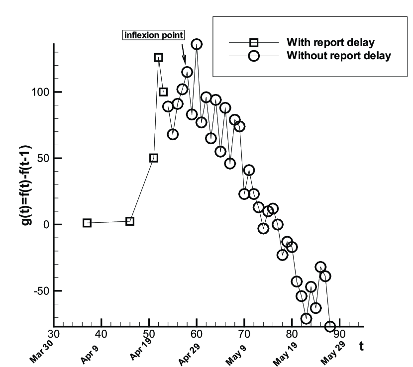
Figure 1: Inflexion point for Beijing. Note that the first peak is not an inflexion point but is simply due to report delay in the early period.

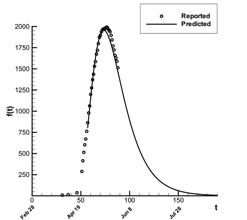
Figure 2: Time history of the number of hospitalized cases for Beijing.

3.2 Test of the model for SARS in 2003

First consider Beijing. Using the reported date as shown in Fig 2, we identify April 27 to be the critical date since $\frac{df(t)}{dt}$ experiences an evident decrease after that date (we also observe a decrease before April 25, but that decrease is due to the report delay). Using the reported date we have $f(L)=980$ and $\left.\frac{df(t)}{dt}\right|_{t=L}=116$. Hence  $L=24$ according to (3.1). This means that the initial date for irregular spread is April 3. Using  (2.6) we predict $D$ and $f(D)$ to be $D=42$ (May 13) and $f(D)=1955$, while according to the report, $D=44$ (May 15) and $f(D)=1991$. The predicted curve $f=f(t)$ follows well the curve, as can be seen in Fig. LABEL:fg2.

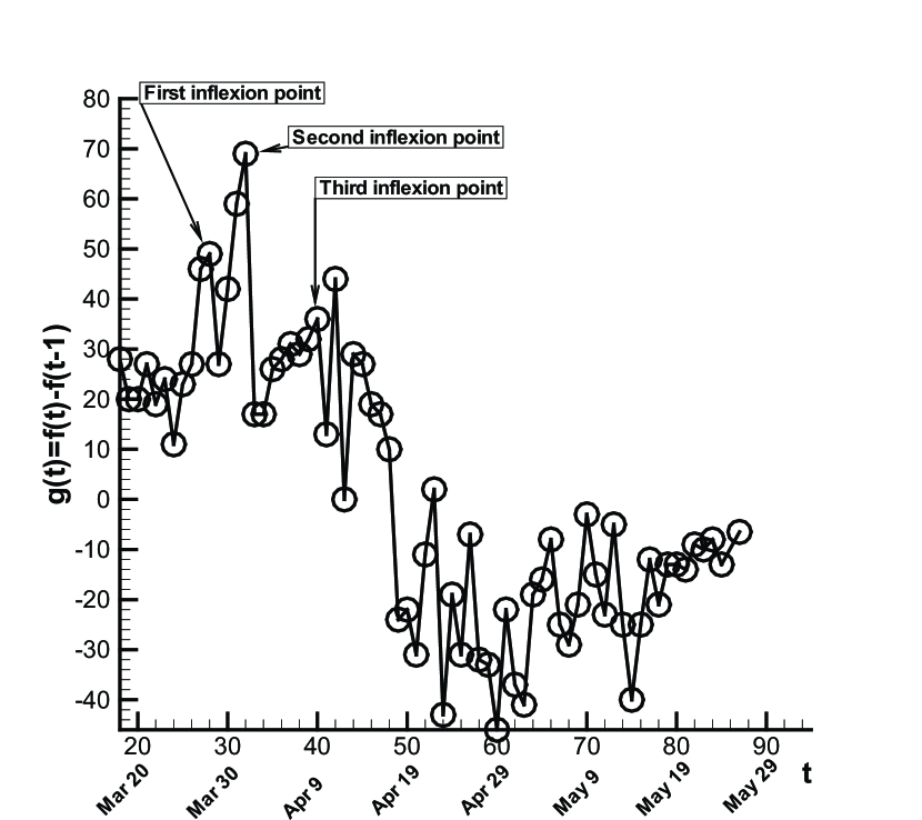
Figure 3: For Hong Kong we observe three distinct inflexion points.

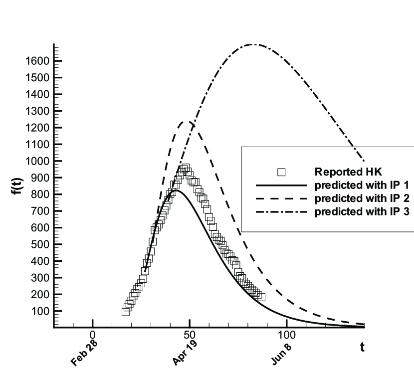
Figure 4: The prediction using the information at the three inflexion points (IP1, IP2, IP3) shows that the predicted curve using the first inflexion point is the closest to the reported data.

For Hong Kong, we observe three distinct inflexion points as can be seen in Fig 4. The prediction using the information at the three inflexion points (IP1, IP2, IP3) show that the predicted curve using the first inflexion point is the closest to the reported data (Fig. 4). More details can be seen in Table 1. In Table 1, when there are multiple inflexion points, as is in the case for Hong Kong, Singapore and Canada, we use the information at the first inflexion point. In the case of Singapore and Canada, there are two maximums but we give information only for the first one.

Table 1: Predicted number $H$ and date $D$ compared with the reported ones for several cities or regions (Mainland refers to Mainland China).

Regions	Inf⋅lexion date			Date $D$		Maximum $H$		Error
	Date	$F$	$G$	Pred	Rep	Pred	Rep
Beijing	Apr27	${\small 980}$	${\small 116}$	May13	May15	${\small 1955}$	${\small 1991}$	2%
HK	Mar28	${\small 960}$	${\small 49}$	Apr12	Apr14	${\small 823}$	${\small 960}$	14%
World	Apr23	${\small 2005}$	${\small 222}$	May9	May12	${\small 4015}$	${\small 3700}$	8.5%
Mainland	Apr27	${\small 1572}$	${\small 177}$	May14	May12	${\small 3332}$	${\small 3068}$	8.6%
Hebei	May4	${\small 92}$	${\small 17}$	May15	May13	${\small 177}$	${\small 161}$	8%
Singap.	Mar18	${\small 29}$	${\small 6}$	Mar27	Mar23	${\small 61}$	${\small 60}$	1%
Canada	Mar27	${\small 49}$	${\small 9}$	Apr10	Apr4	${\small 104}$	${\small 67}$	55%

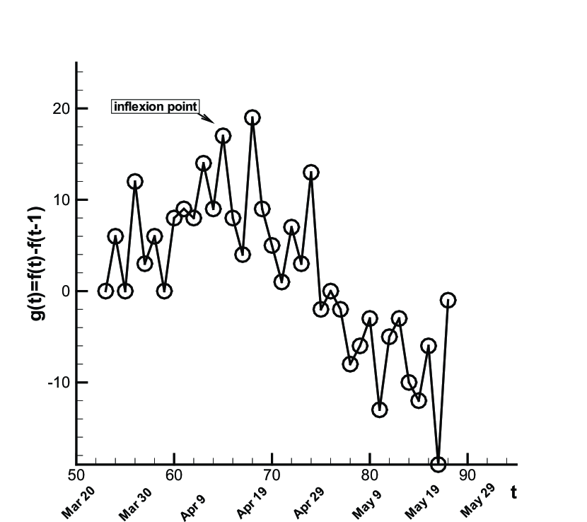
Figure 5: For the Province of Hebei of China the inflexion point is still identifiable.

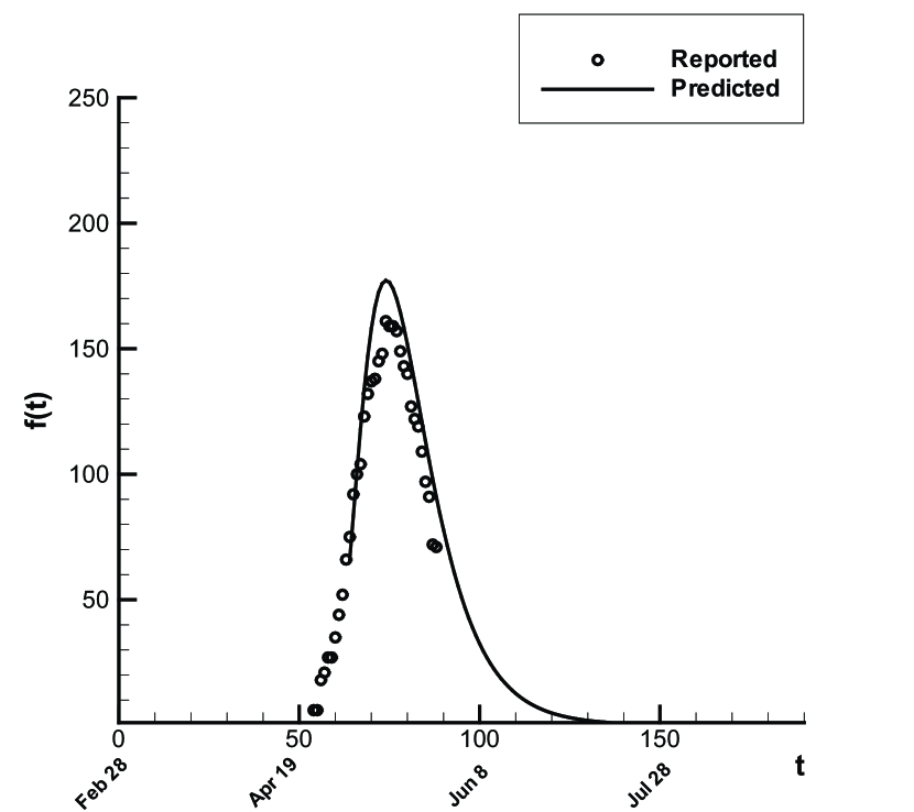
Figure 6: The predicted curve is reasonable as compared to the reported one, though the number of cases in Hebei is not large.

For Hebei, the number of cases is not large. But the prediction still works very well (Fig. 6, Fig. 6).

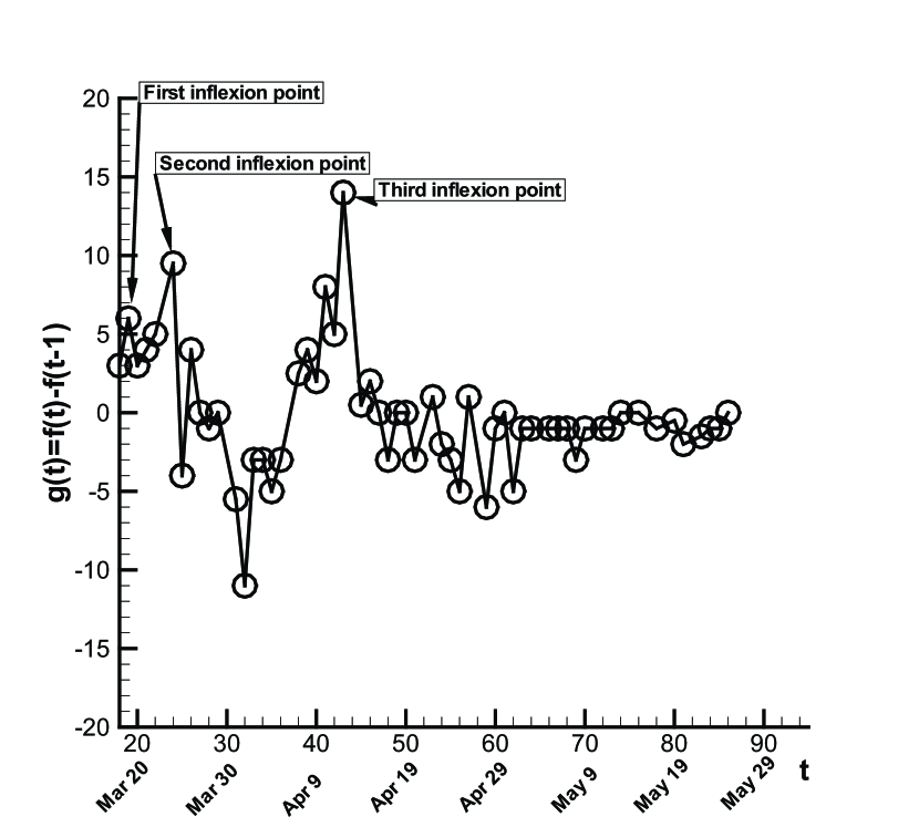
Figure 7: Inflexion points for Singapore.

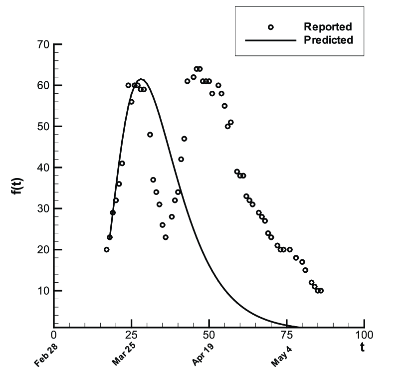
Figure 8: Comparion between predicted and reported cases for Singapore.

For Singapore we observe three distinct inflexion points and two maximums (Fig. 8). The prediction using the information at the first inflexion point fits well to the most part of the first peak (Fig. 8). For Canada we observe two inflexion points (Fig. 10) and when the information of the first inflexion point is used the prediction reproduces well the lower part of the observed curve but fails to predict the peak value (Fig. 10).

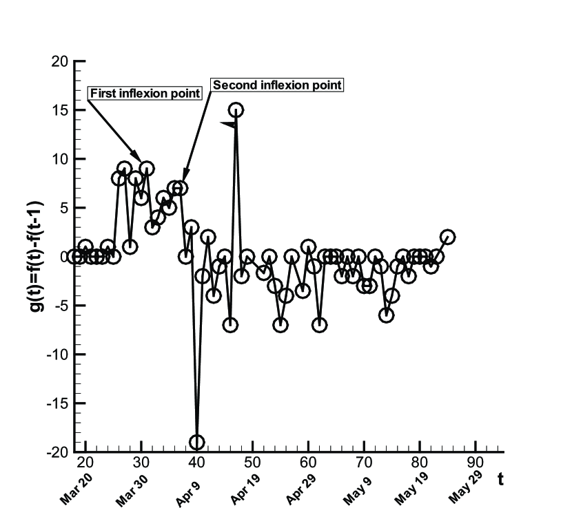
Figure 9: Inflexion points for Canada.

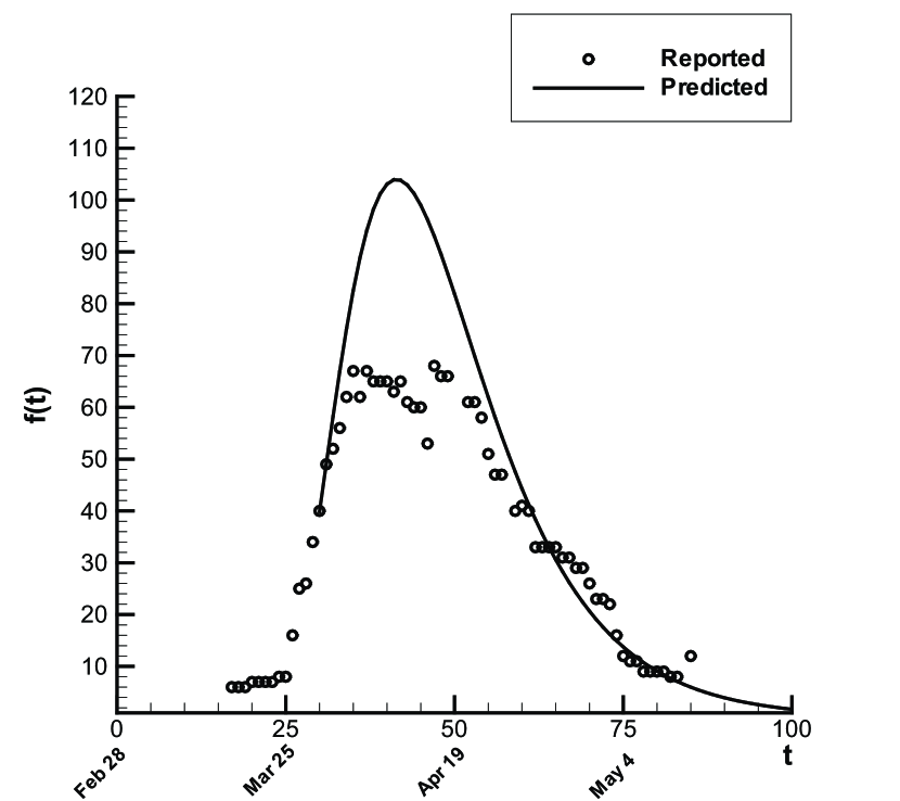
Figure 10: Comparison between predicted and reported cases for Canada.

In summary, when the number is small, the error is large, showing that the thermodynamic approach is more accurate when the system is larger.

3.3 Comparison between the theoretical value of $\sigma$ and the reported value of $\sigma$

It is interesting to note that the best fit value of $\sigma$ using the reported data is close to the theoretical one $(\sigma=0.408)$ (Table 2). In fitting $\sigma$, the date $D$ (counting from the starting date) and the maximum value $H$ are fixed to be the values given by the reported data (third and fourth columns) so that only $\sigma$ is fitted. In the second column, the starting date is approximately the date when the first case was introduced into the region. The outbreak for the epidemic is assumed to take place within at most ten days so the best fit $\sigma$ is obtained by using two epidemic starting days (date with the introduction of the first case and latest possible outbreak date). The range of best fit $\sigma$ (fifth column) is very close to the theoretical value $0.408$ for Beijing and is not significantly different from the theoretical value for the other cities or regions.

Table 2: Best fit value of $\sigma$ for several regions using the least square method, compared to the theoretical value $\sigma=0.408$. The agreement is reasonable.

Regions	Starting date	Date $D$	Maximum $H$	Best f⋅it $\sigma$
Beijing	Mar 25/(10 days later)	May 15	1991	0.349/0.462
Hong Kong	Feb. 20/(10 days later)	Apr. 14	960	0.285/0.343
World	Feb. 20/(10 days later)	May 12	3700	0.273/0.32
Mainland China	Mar 25/(10 days later)	May 12	3068	0.307/0.404
Hebei	Apr. 17/(10 days later)	May 13	161	0.367/0.357
Singapore	March 1/(10 days later)	Apr. 15	64	0.409/0.491
Canada	Feb. 25/(10 days later)	April 8	84	0.297/0.368

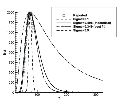
Figure 11: Role of $\sigma$ on the correct reproduction of the curve $f=f(t)$.

One would wonder if the use of a value $\sigma$ far beyond the theoretical value does not alter the curve significantly. In order to see that, we display in Fig. 11 the role of $\sigma$ on the correct reproduction of the curve $f=f(t)$. The log-normal curves using the thermodynamical value $\sigma=0.408$ and the best fit value $\sigma=0.47$ are all close to the reported data. However, when $\sigma$ is significantly different from the thermodynamical value, then the log-normal curve has a great departure from the reported data, as can be seen from the curves using $\sigma=0.1$ and $\sigma=0.9$. This shows that the shape of the curve is quite sensitive to $\sigma$ and the theoretical value of $\sigma$ is indeed a rational one.

4 Concluding remarks

We have built a closed model for which we just need some data for the early period to determine the inflexion point $L$, the number $f(L)$ and the increase rate $df(L)/dt$. The model is applied to predict the number for $t>L$ and especially $D$ and $f(D)$ for the 2003 SARS and is hoped to work when the system for SARS or similar epidemic spread involves multiscale interventions and constitutes a thermodynamical system. Despite the possible uncertainty in the reported data for $0<t<L$ and that the model does not require epidemic details such as latent, incubation and infectious periods, the comparison between model prediction and reported SARS data is still good enough for the cities or regions where the epidemic is severe. The prediction for the case of Beijing is remarkably well since the number of cases is very large. This shows that when the system is large enough, the thermodynamic approach is more accurate. The actual model has some difficulty to exactly handle the case of multiple inflexion points.

The present model can be possibly used to predict epidemics other than SARS once the communicable epidemics receive intensive interventions. The H7N9 avian influenza is actually of great concern [28, 29] and if unluckily this should spread rapidly, we expect the present model would be useful for predicting its spread.

For avian influenza, the observed severe symptom mainly includes high fever and pneumonia [28, 29]. It is interesting to note that, according to traditional Chinese meridian doctrine [30, 31], giving a pressure down or performing an acupuncture on specific acupuncture points on the meridian in a correct way by experts could be helpful to relieve or cure the corresponding symptoms (see Table 3).

Table 3: The symptoms and the corresponding meridian acupuncture points (reproduced from reference [31]). Pain is felt on the meridian acupuncture points while a pressure is given on that points, if the corresponding symptom exists

Symptom	Acupuncture (meridian)	Figure
high fever	zh$\bar{\mathrm{o}}$ngzh$\check{\mathrm{u}}$ (TE3; SJ3),	Fig 12
	ti$\bar{\mathrm{a}}$nf$\check{\mathrm{u}}$ (L3; LU3),
	la$\acute{\mathrm{o}}$g$\bar{\mathrm{o}}$ng (P8; PC8),
	zh$\bar{\mathrm{o}}$ngch$\bar{\mathrm{o}}$ng (P9; PC9),
	d$\grave{\mathrm{a}}$zh$\grave{\mathrm{u}}$ (B11; BL11),
pneumonia	d$\grave{\mathrm{a}}$nzh$\bar{\mathrm{o}}$ng (CV17; RN17),	Fig 13
	d$\grave{\mathrm{a}}$zh$\grave{\mathrm{u}}$ (B11; BL11),
	f$\grave{\mathrm{e}}$ish$\grave{\mathrm{u}}$ (B13; BL13),
	y$\acute{\mathrm{u}}$nm$\acute{\mathrm{e}}$n (L2; LU2),
	y$\acute{\mathrm{u}}$j$\grave{\mathrm{i}}$ (L10; LU10)

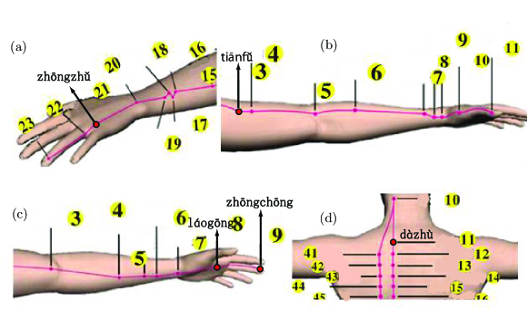
Figure 12: Acupuncture points related to high fever: (a) zh$\bar{\mathrm{o}}$ngzh$\check{\mathrm{u}}$ (shaoyang sanjiao meridian of hand), (b) ti$\bar{\mathrm{a}}$nf$\check{\mathrm{u}}$ (taiyin lung meridian of hand), (c) la$\acute{\mathrm{o}}$g$\bar{\mathrm{o}}$ng and zh$\bar{\mathrm{o}}$ngch$\bar{\mathrm{o}}$ng (jueyin pericardium meridian of hand), (d) d$\grave{\mathrm{a}}$zh$\grave{\mathrm{u}}$ (taiyang bladder meridian of foot).

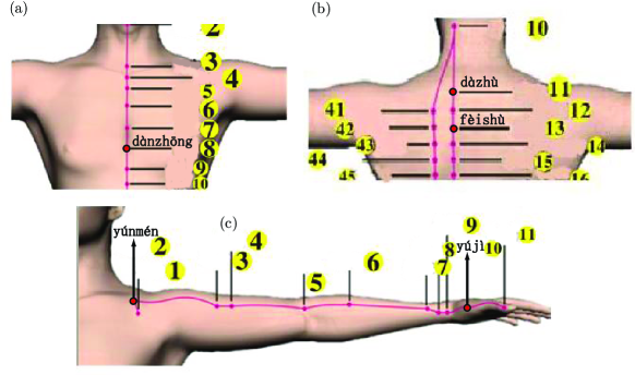
Figure 13: Acupuncture points related to pneumonia: (a) d$\grave{\mathrm{a}}$nzh$\bar{\mathrm{o}}$ng (ren meridian), (b) d$\grave{\mathrm{a}}$zh$\grave{\mathrm{u}}$ and f$\grave{\mathrm{e}}$ish$\grave{\mathrm{u}}$ (taiyang bladder meridian of foot), (c) y$\acute{\mathrm{u}}$nm$\acute{\mathrm{e}}$n and y$\acute{\mathrm{u}}$j$\grave{\mathrm{i}}$ (taiyin lung meridian of hand).

References

- [1] Kamps-Hoffmann, SARS References -05/2003, flying Publishers, see hppt://www.SARSReference.com
- [2] Z. Ma, Y. Zhou and J Wu, Modeling and dynamics of infectious diseases. World Scientific Publishing Co,Inc. 2009.
- [3] C.T. Bauch, J.O. Lloyd-Smith, et al (2005), Dynamically Modeling SARS and Other Newly Emerging Respiratory Illnesses: Past, Present, and Future. Epidemiology, vol.16(6), pp.791-801.
- [4] L. Bian (2012), Spatial Approaches to Modeling Dispersion of Communicable Diseases - A Review, Transactions in GIS, vol 17(1), pp.1-17.
- [5] C.A. Donnelly et al, Epidemiological determinants of spread of causal agent of severe acute respiratory syndrome in Hong Kong, The Lancert, Published online May 7, 2003 (http://image.thelancet.com/extras/03art4432web.pdf)
- [6] S Riley et al, Transmission dynamics of the etiological agent of SARS in Hong Kong: impact of public health interventions, Published online, 23 May 2003; 10.1126/science.1086478
- [7] M. Lipsitch et al, Transmission dynamics and control of severe acute respiratory syndrome, Published online, 23 May 2003; 10.1126/science.1086616
- [8] C. Dye and N. Gay, Modelling the SARS epidemic, Published online, 23 May 2003; 10.1126/science.1086925
- [9] N. Jia and L. Tsui (2005), Epidemic Modelling using Sars as a Case Study, North American Actuarial Journal, vol 9(4), pp.28-42.
- [10] D.J. Watts, R. Muhamad, D.C. Medina, et al (2005), Multiscale, resurgent epidemics in a hierarchical metapopulation model, PNAS, vol 102(32), pp.11157-11162.
- [11] Z.B. Zhang (2007), The outbreak pattern of SARS cases in China as revealed by a mathematical model, Ecological Modelling, vol 204, pp.420-426.
- [12] E. Kenah and J.M. Robins (2007), Second look at the spread of epidemics on networks, Physical Review E, vol 76, 036113.
- [13] L. Bian and D. Liebner (2007), A Network Model for Dispersion of Communicable Diseases, Transactions in GIS, vol 11(2), pp.155-173.
- [14] X.L. Yu, X.Y. Wang, D.M. Zhang, et al (2008), Mathematical expressions for epidemics and immunization in small-world networks, Physica A, vol 387, pp.1421-1430.
- [15] B. Dybiec (2009), SIR mo del of epidemic spread w ith accumulated exp osure, The European Physical Journal B, vol 67, pp.377-383.
- [16] B. Dybiec, A. Kleczkowski and C.A. Gilligan (2009), Modelling control of epidemics spreading by long-range interactions, J. R. Soc. Interface, vol 6, pp.941-950.
- [17] B. Dybiec, A. Kleczkowski and C.A. Gilligan (2009), Modelling control of epidemics spreading by long-range interactions, J. R. Soc. Interface, vol 6, pp.941-950.
- [18] R.M. Anderson and R.M. May (1991), Infectious Diseases of Humans (Oxford Univ. Press,Oxford(1991).
- [19] D. Mollison (Ed.) (1995), Epidemic Models, Cambridge Univ. Press, Cambridge,
- [20] L. Edelstein-Keshet (1988), Mathematical Models in Biology, Random House, New York.
- [21] Z.N. Wu (2003) Prediction of the size distribution of secondary ejected droplets by crown splashing of droplets impinging on a solid wall, Probablistic Engineering Mechanics, vol 18, pp. 241-249.
- [22] F. Brauer and C. Castillo-Chavez (2001), Mathematical Models in Population Biology and Epidemiology, Springer, New York.
- [23] E. Ahmed, H.N. Agiza (1998), On modeling epidemics, including latency, incubation and variable susceptibility, Physica A, vol. 253, pp. 347-352.
- [24] D.Greenhalgh and P.Das (1995), Modeling epidemics with variable contact rates, Theoretical Population Biology, vol. 47, pp.129-179.
- [25] A. Weber, M. Weber, and P. Milligan (2001), Modelling epidemics caused by respiratory syncytial virus, Mathematical Biosciences, vol. 172, 99-113.
- [26] O.G. Pybus, M.A. Charleston, S. Gupta, A. Rambaut, E.C. Holmes, and P.H. Harvey (2001), The Epidemic Behavior of the Hepatitis C Virus, Science, vol. 292, pp. 2323-2325.
- [27] H. Ziegler (1983),An Introduction to Thermomechanics, North-Holland Publ. Company, Amsterdam.
- [28] R.B. Gao, B. Cao, Y.W. Hu, et al (2013), Human Infection with a Novel Avian-Origin Influenza A (H7N9) Virus, The New England Journal of Medicine, online available as http://www.nejm.org/doi/full/10.1056/NEJMoa1304459.
- [29] Y.M. Wen and H.D. Klenk, (2013), H7N9 avian influenza virus - search and re-search, Emerging Microbes and Infections, vol.2, e18, doi:10.1038/emi.2013.18.
- [30] P.H. Rhyu, Acupuncture meridians and acupuncture points.published by AuthorHouse, Bloomington, IN, 2010.
- [31] W.B. Wang, Z.N. Wu, et al, Change-E Health Software based on Acupuncture meridines and Acupuncture points, Software Copyright Register No.201158009625, China, 2011.