Tight Performance Bounds for
Approximate Modified Policy Iteration
with Non-Stationary Policies

Abstract

We consider approximate dynamic programming for the infinite-horizon stationary $\gamma$-discounted optimal control problem formalized by Markov Decision Processes. While in the exact case it is known that there always exists an optimal policy that is stationary, we show that when using value function approximation, looking for a non-stationary policy may lead to a better performance guarantee. We define a non-stationary variant of MPI that unifies a broad family of approximate DP algorithms of the literature. For this algorithm we provide an error propagation analysis in the form of a performance bound of the resulting policies that can improve the usual performance bound by a factor $O\left(1-\gamma\right)$, which is significant when the discount factor $\gamma$ is close to 1. Doing so, our approach unifies recent results for Value and Policy Iteration. Furthermore, we show, by constructing a specific deterministic MDP, that our performance guarantee is tight.

1 Introduction

We consider a discrete-time dynamic system whose state transition depends on a control. We assume that there is a state space $X$. When at some state, an action is chosen from a finite action space $A$. The current state $x\in X$ and action $a\in A$ characterizes through a homogeneous probability kernel $P(dx|x,a)$ the next state’s distribution. At each transition, the system is given a reward $r(x,a,y)\in\mathbb{R}$ where $r:X\times A\times Y\to\mathbb{R}$ is the instantaneous reward function. In this context, we aim at determining a sequence of actions that maximizes the expected discounted sum of rewards from any starting state $x$:

$$\mathbb{E}\left[\left.\sum_{k=0}^{\infty}\gamma^{k}r(x_{k},a_{k},x_{k+1})~{}\right|~{}x_{0}=x,~{}x_{t+1}\sim P(\cdot|x_{t},a_{t}),~{}a_{0},~{}a_{1},~{}\dots\right],$$

where $0<\gamma<1$ is a discount factor. The tuple $\langle X,A,P,r,\gamma\rangle$ is called a Markov Decision Process (MDP) and the associated optimization problem infinite-horizon stationary discounted optimal control (Puterman, 1994; Bertsekas and Tsitsiklis, 1996) .

An important result of this setting is that there exists at least one stationary deterministic policy, that is a function $\pi:X\rightarrow A$ that maps states into actions, that is optimal (Puterman, 1994). As a consequence, the problem is usually recast as looking for the stationary deterministic policy $\pi$ that maximizes for all initial state $x$ the quantity

$$v_{\pi}(x):=\mathbb{E}\left[\left.\sum_{k=0}^{\infty}\gamma^{k}r(x_{k},\pi(x_{k}),x_{k+1})~{}\right|~{}x_{0}=x,~{}x_{t+1}\sim P_{\pi}(\cdot|x_{t})\right],$$ (1)

also called the value of policy $\pi$ at state $x$, and where we wrote $P_{\pi}(dx|x)$ for the stochastic kernel $P(dx|x,\pi(s))$ that chooses actions according to policy $\pi$. We shall similarly write $r_{\pi}:X\to\mathbb{R}$ for the function that giving the immediate reward while following policy $\pi$:

$$\forall x,~{}~{}r_{\pi}(x)=\mathbb{E}\left[r(x_{0},\pi(x_{0}),x_{1})~{}|~{}x_{1}\sim P_{\pi}(\cdot|x_{0})\right].$$

Two linear operators are associated to the stochastic kernel $P_{\pi}$: a left operator on functions

$$\forall f\in\mathbb{R}^{X},~{}~{}\forall x\in X,~{}~{}(P_{\pi}f)(x)=\int f(y)P_{\pi}(dy|x)=\mathbb{E}\left[f(x_{1})~{}|~{}x_{1}\sim P_{\pi}(\cdot|x_{0})\right],$$

and a right operator on distributions:

$$\forall\mu,~{}~{}(\mu P_{\pi})(dy)=\int P_{\pi}(dy|x)\mu(dx).$$

In words, $P_{\pi}f(x)$ is the expected value of $f$ after following policy $\pi$ for a single time-step starting from $x$, and $\mu P_{\pi}$ is the distribution of states after a single time-step starting from $\mu$.

Given a policy $\pi$, it is well known that the value $v_{\pi}$ is the unique solution of the following Bellman equation:

$$v_{\pi}=r_{\pi}+\gamma P_{\pi}v_{\pi}.$$

In other words, $v_{\pi}$ is the fixed point of the affine operator $T_{\pi}v:=r_{\pi}+\gamma P_{\pi}v$.

The optimal value starting from state $x$ is defined as

$$v_{*}(x):=\max_{\pi}v_{\pi}(x).$$

It is also well known that $v_{*}$ is characterized by the following Bellman equation:

$$v_{*}=\max_{\pi}(r_{\pi}+\gamma P_{\pi}v_{*})=\max_{\pi}T_{\pi}v_{*},$$

where the max operator is componentwise. In other words, $v_{*}$ is the fixed point of the nonlinear operator $Tv:=\max_{\pi}T_{\pi}v$. For any value vector $v$, we say that a policy $\pi$ is greedy with respect to the value $v$ if it satisfies:

$$\pi\in\arg\max_{\pi^{\prime}}T^{\pi^{\prime}}v$$

or equivalently $T_{\pi}v=Tv$. We write, with some abuse of notation $\mathcal{G}(v)$ any policy that is greedy with respect to $v$. The notions of optimal value function and greedy policies are fundamental to optimal control because of the following property: any policy $\pi_{*}$ that is greedy with respect to the optimal value is an optimal policy and its value $v_{\pi_{*}}$ is equal to $v_{*}$.

Given an MDP, we consider approximate versions of the Modified Policy Iteration (MPI) algorithm (Puterman and Shin, 1978). Starting from an arbitrary value function $v_{0}$, MPI generates a sequence of value-policy pairs

$$\pi_{k+1} =\mathcal{G}(v_{k})$$ (greedy step)

$$v_{k+1} =(T_{\pi_{k+1}})^{m+1}v_{k}+\epsilon_{k}$$ (evaluation step)

where $m\geq 0$ is a free parameter. At each iteration $k$, the term $\epsilon_{k}$ accounts for a possible approximation in the evaluation step. MPI generalizes the well-known dynamic programming algorithms Value Iteration (VI) and Policy Iteration (PI) for values $m=0$ and $m=\infty$, respectively. In the exact case ($\epsilon_{k}=0$), MPI requires less computation per iteration than PI (in a way similar to VI) and enjoys the faster convergence (in terms of number of iterations) of PI (Puterman and Shin, 1978; Puterman, 1994).

It was recently shown that controlling the errors $\epsilon_{k}$ when running MPI is sufficient to ensure some performance guarantee (Scherrer and Thiery, 2010; Scherrer et al., 2012a, b; Canbolat and Rothblum, 2012). For instance, we have the following performance bound, that is remarkably independent of the parameter $m$.

Theorem 1 (Scherrer et al. (2012a, Remark 2)).

Consider MPI with any parameter $m\geq 0$. Assume there exists an $\epsilon>0$ such that the errors satisfy $\|\epsilon_{k}\|_{\infty}<\epsilon$ for all $k$. Then, the loss due to running policy $\pi_{k}$ instead of the optimal policy $\pi_{*}$ satisfies

$${\left\lVert v_{*}-v_{\pi_{k}}\right\rVert}_{\infty}\leq\frac{2(\gamma-\gamma^{k})}{(1-\gamma)^{2}}\epsilon+\frac{2\gamma^{k}}{1-\gamma}{\left\lVert v_{*}-v_{0}\right\rVert}_{\infty}.$$

In the specific case corresponding to VI ($m=0$) and PI ($m=\infty$), this bound matches performance guarantees that have been known for a long time (Singh and Yee, 1994; Bertsekas and Tsitsiklis, 1996). The constant $\frac{2\gamma}{(1-\gamma)^{2}}$ can be very big, in particular when $\gamma$ is close to $1$, and consequently the above bound is commonly believed to be conservative for practical applications. Unfortunately, this bound cannot be improved: Bertsekas and Tsitsiklis (1996, Example 6.4) showed that the bound is tight for PI, Scherrer and Lesner (2012) proved that it is tight for VI, and we will prove in this article the—to our knowledge unknown—fact that it is also tight for MPI. In other words, improving the performance bound requires to change the algorithms.

2 Main Results

Even though the theory of optimal control states that there exists a stationary policy that is optimal, Scherrer and Lesner (2012) recently showed that the performance bound of Theorem 1 could be improved in the specific cases $m=0$ and $m=\infty$ by considering variations of VI and PI that build periodic non-stationary policies (instead of stationary policies). In this article, we consider an original MPI algorithm that generalizes these variations of VI and PI (in the same way the standard MPI algorithm generalizes standard VI and PI). Given some free parameters $m\geq 0$ and $\ell\geq 1$, an arbitrary value function $v_{0}$ and an arbitrary set of $\ell-1$ policies $\pi_{0},\pi_{-1},\pi_{-\ell+2}$, consider the algorithm that builds a sequence of value-policy pairs as follows:

$$\pi_{k+1} =\mathcal{G}(v_{k})$$ (greedy step)

$$v_{k+1} =(T_{\pi_{k+1,\ell}})^{m}T_{\pi_{k+1}}v_{k}+\epsilon_{k}.$$ (evaluation step)

While the greedy step is identical to the one of the standard MPI algorithm, the evaluation step involves two new objects that we describe now. $\pi_{k+1,\ell}$ denotes the periodic non-stationary policy that loops in reverse order on the last $\ell$ generated policies:

$$\pi_{k+1,\ell}=\underbrace{\pi_{k+1}\ \pi_{k}\ \cdots\ \pi_{k-\ell+2}}_{{\tiny\mbox{last $\ell$ policies}}}~{}\underbrace{\pi_{k+1}\ \pi_{k}\ \cdots\ \pi_{k-\ell+2}}_{{\tiny\mbox{last $\ell$ policies}}}\cdots$$

Following the policy $\pi_{k+1,\ell}$ means that the first action is selected by $\pi_{k+1}$, the second one by $\pi_{k}$, until the $\ell^{\mathrm{th}}$ one by $\pi_{k-\ell+2}$, then the policy loops and the next actions are selected by $\pi_{k+1}$, $\pi_{k}$, so on and so forth. In the above algorithm, $T_{\pi_{k+1,\ell}}$ is the linear Bellman operator associated to $\pi_{k+1,\ell}$:

$$T_{\pi_{k+1,l}}=T_{\pi_{k+1}}T_{\pi_{k}}\dots T_{\pi_{k-\ell+2}},$$

that is the operator of which the unique fixed point is the value function of $\pi_{k+1,\ell}$. After $k$ iterations, the output of the algorithm is the periodic non-stationary policy $\pi_{k,\ell}$.

For the values $m=0$ and $m=\infty$, one respectively recovers the variations of VI and PI recently proposed by Scherrer and Lesner (2012). When $\ell=1$, one recovers the standard MPI algorithm by Puterman and Shin (1978) (that itself generalizes the standard VI and PI algorithm). As it generalizes all previously proposed algorithms, we will simply refer to this new algorithm as MPI with parameters $m$ and $\ell$.

On the one hand, using this new algorithm may require more memory since one must store $\ell$ policies instead of one. On the other hand, our first main result, proved in Section 4, shows that this extra memory allows to improve the performance guarantee.

Theorem 2.

Consider MPI with any parameters $m\geq 0$ and $\ell\geq 1$. Assume there exists an $\epsilon>0$ such that the errors satisfy $\|\epsilon_{k}\|_{\infty}<\epsilon$ for all $k$. Then, the loss due to running policy $\pi_{k,\ell}$ instead of the optimal policy $\pi_{*}$ satisfies

$${\left\lVert v_{*}-v_{\pi_{k,\ell}}\right\rVert}_{\infty}\leq\frac{2(\gamma-\gamma^{k})}{(1-\gamma)(1-\gamma^{\ell})}\epsilon+\frac{2\gamma^{k}}{1-\gamma}{\left\lVert v_{*}-v_{0}\right\rVert}_{\infty}.$$

As already observed for the standard MPI algorithm, this performance bound is independent of $m$. For any $\ell\geq 1$, it is a factor $\frac{1-\gamma}{1-\gamma^{\ell}}$ better than in Theorem 1. Using $\ell=\left\lceil\frac{1}{1-\gamma}\right\rceil$ yields a performance bound of

$${\left\lVert v_{*}-v_{\pi_{k,\ell}}\right\rVert}_{\infty}<\frac{3.164(\gamma-\gamma^{k})}{1-\gamma}\epsilon+\frac{2\gamma^{k}}{1-\gamma}{\left\lVert v_{*}-v_{0}\right\rVert}_{\infty},$$

and constitutes asymptotically an improvement of order $O(1-\gamma)$, which is significant when $\gamma$ is close to 1. In fact, Theorem 2 is a generalization of Theorem 1 for $\ell>1$ (the bounds match when $\ell=1$). While this result was obtained through two independent proofs for the variations of VI and PI proposed by Scherrer and Lesner (2012), the more general setting that we consider here involves a unified proof that extends that provided for the standard MPI ($\ell=1$) by Scherrer et al. (2012b). Moreover, our result is much more general since it applies to all the variations of MPI for any $\ell$ and $m$.

Figure 1: The deterministic MDP matching the bound of Theorem 2.

The second main result of this article, proved in Section 5, is that the bound of Theorem 2 is tight, in the precise sense formalized by the following theorem.

Theorem 3.

For all parameter values $m\geq 0$ and $\ell\geq 1$, for all $\epsilon>0$, there exists an MDP instance, an initial value function $v_{0}$, a set of initial policies $\pi_{0},\pi_{-1},\dots,\pi_{-\ell+2}$ and a sequence of error terms $(\epsilon_{k})_{k\geq 1}$ satisfying $\|\epsilon_{k}\|_{\infty}\leq\epsilon$, such that for all iterations $k$, the bound of Theorem 2 is satisfied with equality.

This theorem generalizes the (separate) tightness results for PI (Bertsekas and Tsitsiklis, 1996) and for VI (Scherrer and Lesner, 2012) where the problem constructed to attain the bound is a specialization of the one we use in Section 5. To our knowledge, this result is new even for the standard MPI algorithm ($m$ arbitrary but $\ell=1$), and for the non-trivial non-stationary variations of VI ($m=0$, $\ell>1$) and PI ($m=\infty$, $\ell>1$). The proof considers a generalization of the MDP instance used to prove the tightness of the bound for VI (Scherrer and Lesner, 2012) and PI (Bertsekas and Tsitsiklis, 1996, Example 6.4). Precisely, this MDP consists of states $\{1,2,\dots\}$, two actions: left ($\leftarrow$) and right ($\rightarrow$); the reward function $r$ and transition kernel $P$ are characterized as follows for any state $i\geq 2$:

$$r(i,\leftarrow) =0, r(i,\rightarrow) =-2\frac{\gamma-\gamma^{i}}{1-\gamma}\epsilon,$$

$$P(i|i+1,\leftarrow) =1, P(i+\ell-1|i,\rightarrow) =1,$$

and $r(1)=0$ and $P(1|1)1$ for state $1$ (all the other transitions having zero probability mass). As a shortcut, we will use the notation $r_{i}$ for the non-zero reward $r(i,\rightarrow)$ in state $i$. Figure 1 depicts the general structure of this MDP. It is easily seen that the optimal policy $\pi_{*}$ is to take $\leftarrow$ in all states $i\geq 2$, as doing otherwise would incur a negative reward. Therefore, the optimal value $v_{*}(i)$ is $0$ in all states $i$. The proof of the above theorem considers that we run MPI with $v_{0}=v_{*}=0$, $\pi_{0}=\pi_{-1}=\dots=\pi_{\ell+2}=\pi_{*}$, and the following sequence of error terms:

$$\forall i,~{}~{}\epsilon_{k}(i)=\left\{\begin{array}[]{ll}-\epsilon&\text{if }i=k,\\ \epsilon&\text{if }i=k+\ell,\\ 0&\text{otherwise}.\end{array}\right.$$

In such a case, one can prove that the sequence of policies $\pi_{1},\pi_{2},\dots,\pi_{k}$ that are generated up to iteration $k$ is such that for all $i\leq k$, the policy $\pi_{i}$ takes $\leftarrow$ in all states but $i$, where it takes $\rightarrow$. As a consequence, a non-stationary policy $\pi_{k,\ell}$ built from this sequence takes $\rightarrow$ in $k$ (as dictated by $\pi_{k}$), which transfers the system into state $k+\ell-1$ incurring a reward of $r_{k}$. Then the policies $\pi_{k-1},\pi_{k-2},\dots,\pi_{k-\ell+1}$ are followed, each indicating to take $\leftarrow$ with $0$ reward. After $\ell$ steps, the system is again is state $k$ and, by the periodicity of the policy, must again use the action $\pi_{k}(k)=\ \rightarrow$. The system is thus stuck in a loop, where every $\ell$ steps a negative reward of $r_{k}$ is received. Consequently, the value of this policy from state $k$ is:

$$v_{\pi_{k,\ell}}(k)=r_{k}+\gamma^{\ell}(r_{k}+\gamma^{\ell}(r_{k}+\cdots)\cdots)=\frac{r_{k}}{1-\gamma^{\ell}}=-\frac{\gamma-\gamma^{k}}{(1-\gamma)(1-\gamma^{\ell})}2\epsilon.$$

As a consequence, we get the following lower bound,

$${\left\lVert v_{*}-v_{\pi_{k,\ell}}\right\rVert}_{\infty}\geq|v_{\pi_{k,\ell}}(k)|=\frac{\gamma-\gamma^{k}}{(1-\gamma)(1-\gamma^{\ell})}2\epsilon$$

which exactly matches the upper bound of Theorem 2 (since $v_{0}=v_{*}=0$). The proof of this result involves computing the values $v_{k}(i)$ for all states $i$, steps $k$ of the algorithm, and values $m$ and $\ell$ of the parameters, and proving that the policies $\pi_{k+1}$ that are greedy with respect to these values satisfy what we have described above. Because of the cyclic nature of the MDP, the shape of the value function is quite complex—see for instance Figures 2 and 3 in Section 5—and the exact derivation is tedious. For clarity, this proof is deferred to Section 5.

3 Discussion

Since it is well known that there exists an optimal policy that is stationary, our result—as well as those of Scherrer and Lesner (2012)—suggesting to consider non-stationary policies may appear strange. There exists, however, a very simple approximation scheme of discounted infinite-horizon control problems—that has to our knowledge never been documented in the literature—that sheds some light on the deep reason why non-stationary policies may be an interesting option. Given an infinite-horizon problem, consider approximating it by a finite-horizon discounted control problem by “cutting the horizon” after some sufficiently big instant $T$ (that is assume there is no reward after time $T$). Contrary to the original infinite-horizon problem, the resulting finite-horizon problem is non-stationary, and has therefore naturally a non-stationary solution that is built by dynamic programming in reverse order. Moreover, it can be shown (Kakade, 2003, by adapting the proof of Theorem 2.5.1) that solving this finite-horizon with VI with a potential error of $\epsilon$ at each iteration, will induce at most a performance error of $2\sum_{i=0}^{T-1}\gamma^{t}\epsilon=\frac{2(1-\gamma^{T})}{1-\gamma}\epsilon$. If we add the error due to truncating the horizon ($\gamma^{T}\frac{\max_{s,a}|r(s,a)|}{1-\gamma}$), we get an overall error of order $O\left(\frac{1}{1-\gamma}\epsilon\right)$ for a memory $T$ of the order of $\tilde{O}\left(\frac{1}{1-\gamma}\right)$. Though this approximation scheme may require a significant amount of memory (when $\gamma$ is close to $1$), it achieves the same $O(1-\gamma)$ improvement over the standard MPI performance bound as our MPI new scheme proposed through our generalization of MPI with two parameters $m$ and $\ell$. In comparison, the new proposed algorithm can be seen as a more flexible way to make the trade-off between the memory and the quality.

A practical limitation of Theorem 2 is that it assumes that the errors $\epsilon_{k}$ are controlled in max norm. In practice, the evaluation step of dynamic programming algorithm is usually done through some regression scheme—see for instance (Bertsekas and Tsitsiklis, 1996; Antos et al., 2007a, b; Scherrer et al., 2012a)—and thus controlled through some weighted quadratic $L_{2,\mu}$ norm, defined as $\|f\|_{2,\mu}=\sqrt{\int f(x)\mu(dx)}$. Munos (2003, 2007) originally developed such analyzes for VI and PI. Farahmand et al. (2010) and Scherrer et al. (2012a) later improved it. Using a technical lemma due to Scherrer et al. (2012a, Lemma 3), one can easily deduce from our analysis (developed in Section 4) the following performance bound.

Corollary 1.

Consider MPI with any parameters $m\geq 0$ and $\ell\geq 1$. Assume there exists an $\epsilon>0$ such that the errors satisfy $\|\epsilon_{k}\|_{2,\mu}<\epsilon$ for all $k$. Then, the expected (with respect to some initial measure $\rho$) loss due to running policy $\pi_{k,\ell}$ instead of the optimal policy $\pi_{*}$ satisfies

$$\mathbb{E}\left[v_{*}(s)-v_{\pi_{k,\ell}}(s)~{}|~{}s\sim\rho\right]\leq\frac{2(\gamma-\gamma^{k})C_{1,k,\ell}}{(1-\gamma)(1-\gamma^{\ell})}\epsilon+\frac{2\gamma^{k}C_{k,k+1,1}}{1-\gamma}{\left\lVert v_{*}-v_{0}\right\rVert}_{2,\mu},$$

where

$$C_{j,k,l}=\frac{(1-\gamma)(1-\gamma^{l})}{\gamma^{j}-\gamma^{k}}\sum_{i=j}^{k-1}\sum_{n=i}^{\infty}\gamma^{i+ln}c(i+ln)$$

is a convex combination of concentrability coefficients based on Radon-Nikodym derivatives

$$c(j)=\max_{\pi_{1},\cdots,\pi_{j}}\left\|\frac{d(\rho P_{\pi_{1}}P_{\pi_{2}}\cdots P_{\pi_{j}})}{d\mu}\right\|_{2,\mu}.$$

With respect to the previous bound in max norm, this bound involves extra constants $C_{j,k,l}\geq 1$. Each such coefficient $C_{j,k,l}$ is a convex combination of terms $c(i)$, that each quantifies the difference between 1) the distribution $\mu$ used to control the errors and 2) the distribution obtained by starting from $\rho$ and making $k$ steps with arbitrary sequences of policies. Overall, this extra constant can be seen as a measure of stochastic smoothness of the MDP (the smoother, the smaller). Further details on these coefficients can be found in (Munos, 2003, 2007; Farahmand et al., 2010).

The next two sections contain the proofs of our two main results, that are Theorem 2 and 3.

4 Proof of Theorem 2

Throughout this proof we will write $P_{k}$ (resp. $P_{*}$) for the transition kernel $P_{\pi_{k}}$ (resp. $P_{\pi_{*}}$) induced by the stationary policy $\pi_{k}$ (resp. $\pi_{*}$). We will write $T_{k}$ (resp. $T_{*}$) for the associated Bellman operator. Similarly, we will write $P_{k,\ell}$ for the transition kernel associated with the non-stationary policy $\pi_{k,\ell}$ and $T_{k,\ell}$ for its associated Bellman operator.

For $k\geq 0$ we define the following quantities:

• $b_{k}=T_{k+1}v_{k}-T_{k+1,\ell}T_{k+1}v_{k}$. This quantity which we will call the residual may be viewed as a non-stationary analogue of the Bellman residual $v_{k}-T_{k+1}v_{k}$.

• $s_{k}=v_{k}-v_{\pi_{k,\ell}}-\epsilon_{k}$. We will call it shift, as it measures the shift between the value $v_{\pi_{k,\ell}}$ and the estimate $v_{k}$ before incurring the error.

• $d_{k}=v_{*}-v_{k}+\epsilon_{k}$. This quantity, called distance thereafter, provides the distance between the $k^{\text{th}}$ value function (before the error is added) and the optimal value function.

• $l_{k}=v_{*}-v_{\pi_{k,\ell}}$. This is the loss of the policy $v_{\pi_{k,\ell}}$. The loss is always non-negative since no policy can have a value greater than or equal to $v_{*}$.

The proof is outlined as follows. We first provide a bound on $b_{k}$ which will be used to express both the bounds on $s_{k}$ and $d_{k}$. Then, observing that $l_{k}=s_{k}+d_{k}$ will allow to express the bound of ${\left\lVert l_{k}\right\rVert}_{\infty}$ stated by Theorem 2. Our arguments extend those made by Scherrer et al. (2012a) in the specific case $\ell=1$.

We will repeatedly use the fact that since policy $\pi_{k+1}$ is greedy with respect to $v_{k}$, we have

$$\forall\pi^{\prime},~{}~{}T_{k+1}v_{k}\geq T_{\pi^{\prime}}v_{k}.$$ (2)

For a non-stationary policy $\pi_{k,\ell},$ the induced $\ell$-step transition kernel is

$$P_{k,\ell}=P_{k}P_{k-1}\cdots P_{k-\ell+1}.$$

As a consequence, for any function $f:\mathcal{S}\rightarrow\mathbb{R}$, the operator $T_{k,\ell}$ may be expressed as:

$$T_{k,\ell}f=r_{k}+\gamma P_{k,1}r_{k-1}+\gamma^{2}P_{k,2}r_{k-2}+\cdots+\gamma^{\ell-1}P_{k,\ell-1}r_{k-\ell+1}+\gamma^{\ell}P_{k,\ell}f$$

then, for any function $g:\mathcal{S}\rightarrow\mathbb{R}$, we have

$$T_{k,\ell}f-T_{k,\ell}g=\gamma^{\ell}P_{{k,\ell}}(f-g)$$ (3)

and

$$T_{k,\ell}(f+g)=T_{k,\ell}f+\gamma^{\ell}P_{{k,\ell}}(g).$$ (4)

The following notation will be useful.

Definition 1 (Scherrer et al. (2012a)).

For a positive integer $n$, we define $\mathbb{P}_{n}$ as the set of discounted transition kernels that are defined as follows:

1. for any set of $n$ policies $\{\pi_{1},\dots,\pi_{n}\}$, $(\gamma P_{\pi_{1}})(\gamma P_{\pi_{2}})\cdots(\gamma P_{\pi_{n}})\in\mathbb{P}_{n}$,

2. for any $\alpha\in(0,1)$ and $P_{1},P_{2}\in\mathbb{P}_{n}$, $\alpha P_{1}+(1-\alpha)P_{2}\in\mathbb{P}_{n}$

With some abuse of notation, we write $\Gamma^{n}$ for denoting any element of $\mathbb{P}_{n}$.

Example 1 ($\Gamma^{n}$ notation).

If we write a transition kernel $P$ as $P=\alpha_{1}\Gamma^{i}+\alpha_{2}\Gamma^{j}\Gamma^{k}=\alpha_{1}\Gamma^{i}+\alpha_{2}\Gamma^{j+k}$, it should be read as: “There exists $P_{1}\in\mathbb{P}_{i}$,$P_{2}\in\mathbb{P}_{j}$,$P_{3}\in\mathbb{P}_{k}$ and $P_{4}\in\mathbb{P}_{j+k}$ such that $P=\alpha_{1}P_{1}+\alpha_{2}P_{2}P_{3}=\alpha_{1}P_{1}+\alpha_{2}P_{4}$.”.

We first provide three lemmas bounding the residual, the shift and the distance, respectively.

Lemma 1 (residual bound).

The residual $b_{k}$ satisfies the following bound:

$$b_{k}\leq\sum_{i=1}^{k}\Gamma^{(\ell m+1)(k-i)}x_{i}+\Gamma^{(\ell m+1)k}b_{0}$$

where

$$x_{k}=(I-\Gamma^{\ell})\Gamma\epsilon_{k}.$$

Proof.

We have:

$$b_{k} =T_{k+1}v_{k}-T_{k+1,\ell}T_{k+1}v_{k}$$

$$\leq T_{k+1}v_{k}-T_{k+1,\ell}T_{k-\ell+1}v_{k} \{T_{k+1}v_{k}\geq T_{k-\ell+1}v_{k}~{}\eqref{eq:g}\}$$

$$=T_{k+1}v_{k}-T_{k+1}T_{k,\ell}v_{k}$$

$$=\gamma P_{{k+1}}\left(v_{k}-T_{k,\ell}v_{k}\right)$$

$$=\gamma P_{{k+1}}\left((T_{k,\ell})^{m}T_{k}v_{k-1}+\epsilon_{k}-T_{k,\ell}\left((T_{k,\ell})^{m}T_{k}v_{k-1}+\epsilon_{k}\right)\right)$$

$$=\gamma P_{{k+1}}\left((T_{k,\ell})^{m}T_{k}v_{k-1}-(T_{k,\ell})^{m+1}T_{k}v_{k-1}+(I-\gamma^{\ell}P_{{k,\ell}})\epsilon_{k}\right) \{\eqref{eq:f+g}\}$$

$$=\gamma P_{{k+1}}\left((\gamma^{\ell}P_{{k,\ell}})^{m}\left(T_{k}v_{k-1}-T_{k,\ell}T_{k}v_{k-1}\right)+(I-\gamma^{\ell}P_{{k,\ell}})\epsilon_{k}\right) \{\eqref{eq:f-g}\}$$

$$=\gamma P_{{k+1}}\left((\gamma^{\ell}P_{{k,\ell}})^{m}b_{k-1}+(I-\gamma^{\ell}P_{{k,\ell}})\epsilon_{k}\right).$$

Which can be written as

$$b_{k}\leq\Gamma(\Gamma^{\ell m}b_{k-1}+(I-\Gamma^{\ell})\epsilon_{k})=\Gamma^{\ell m+1}b_{k-1}+x_{k}.$$

Then, by induction:

$$b_{k}\leq\sum_{i=0}^{k-1}\Gamma^{(\ell m+1)i}x_{k-i}+\Gamma^{(\ell m+1)k}b_{0}=\sum_{i=1}^{k}\Gamma^{(\ell m+1)(k-i)}x_{i}+\Gamma^{(\ell m+1)k}b_{0}.$$

∎

Lemma 2 (distance bound).

The distance $d_{k}$ satisfies the following bound:

$$d_{k}\leq\sum_{i=1}^{k}\sum_{j=0}^{mi-1}\Gamma^{\ell j+i-1}x_{k-i}+\sum_{i=1}^{k}\Gamma^{i-1}y_{k-i}+z_{k},$$

where

$$y_{k}=-\Gamma\epsilon_{k}$$

and

$$z_{k}=\sum_{i=0}^{mk-1}\Gamma^{k-1+\ell i}b_{0}+\Gamma^{k}d_{0}.$$

Proof.

First expand $d_{k}$:

$$d_{k} =v_{*}-v_{k}+\epsilon_{k}$$

$$=v_{*}-(T_{k,\ell})^{m}T_{k}v_{k-1}$$

$$\begin{split}&=v_{*}-T_{k}v_{k-1}+T_{k}v_{k-1}-T_{k,\ell}T_{k}v_{k-1}+T_{k,\ell}T_{k}v_{k-1}-(T_{k,\ell})^{2}T_{k}v_{k-1}\\[8.5359pt] &\quad+(T_{k,\ell})^{2}T_{k}v_{k-1}-\cdots-(T_{k,\ell})^{m-1}T_{k}v_{k-1}+(T_{k,\ell})^{m-1}T_{k}v_{k-1}-(T_{k,\ell})^{m}T_{k}v_{k-1}\end{split}$$

$$=v_{*}-T_{k}v_{k-1}+\sum_{i=0}^{m-1}(T_{k,\ell})^{i}T_{k}v_{k-1}-(T_{k,\ell})^{i+1}T_{k}v_{k-1}$$

$$=T_{*}v_{*}-T_{k}v_{k-1}+\sum_{i=0}^{m-1}(\gamma^{\ell}P_{{k,\ell}})^{i}\left(T_{k}v_{k-1}-T_{k,\ell}T_{k}v_{k-1}\right) \{\eqref{eq:f-g}\}$$

$$\leq T_{*}v_{*}-T_{*}v_{k-1}+\sum_{i=0}^{m-1}(\gamma^{\ell}P_{{k,\ell}})^{i}b_{k-1} \{T_{k}v_{k-1}\geq T_{*}v_{k-1}~{}\eqref{eq:g}\}$$

$$=\gamma P_{{*}}(v_{*}-v_{k-1})+\sum_{i=0}^{m-1}(\gamma^{\ell}P_{{k,\ell}})^{i}b_{k-1} \{\eqref{eq:f-g}\}$$

$$=\gamma P_{{*}}d_{k-1}-\gamma P_{{*}}\epsilon_{k-1}+\sum_{i=0}^{m-1}(\gamma^{\ell}P_{{k,\ell}})^{i}b_{k-1} \{d_{k}=v_{*}-v_{k}+\epsilon_{k}\}$$

$$=\Gamma d_{k-1}+y_{k-1}+\sum_{i=0}^{m-1}\Gamma^{\ell i}b_{k-1}.$$

Then, by induction

$$d_{k}\leq\sum_{j=0}^{k-1}\Gamma^{k-1-j}\left(y_{j}+\sum_{p=0}^{m-1}\Gamma^{\ell p}b_{j}\right)+\Gamma^{k}d_{0}.$$

Using the bound on $b_{k}$ from Lemma 1 we get:

$$d_{k} \leq\sum_{j=0}^{k-1}\Gamma^{k-1-j}\left(y_{j}+\sum_{p=0}^{m-1}\Gamma^{\ell p}\left(\sum_{i=1}^{j}\Gamma^{(\ell m+1)(j-i)}x_{i}+\Gamma^{(\ell m+1)j}b_{0}\right)\right)+\Gamma^{k}d_{0}$$

$$=\sum_{j=0}^{k-1}\sum_{p=0}^{m-1}\sum_{i=1}^{j}\Gamma^{k-1-j+\ell p+(\ell m+1)(j-i)}x_{i}+\sum_{j=0}^{k-1}\sum_{p=0}^{m-1}\Gamma^{k-1-j+\ell p+(\ell m+1)j}b_{0}+\Gamma^{k}d_{0}+\sum_{i=1}^{k}\Gamma^{i-1}y_{k-i}.$$

First we have:

$$\sum_{j=0}^{k-1}\sum_{p=0}^{m-1}\sum_{i=1}^{j}\Gamma^{k-1-j+\ell p+(\ell m+1)(j-i)}x_{i} =\sum_{i=1}^{k-1}\sum_{j=i}^{k-1}\sum_{p=0}^{m-1}\Gamma^{k-1+\ell(p+mj)-i(\ell m+1)}x_{i}$$

$$=\sum_{i=1}^{k-1}\sum_{j=0}^{m(k-i)-1}\Gamma^{k-1+\ell(j+mi)-i(\ell m+1)}x_{i}$$

$$=\sum_{i=1}^{k-1}\sum_{j=0}^{m(k-i)-1}\Gamma^{\ell j+k-i-1}x_{i}$$

$$=\sum_{i=1}^{k-1}\sum_{j=0}^{mi-1}\Gamma^{\ell j+i-1}x_{k-i}.$$

Second we have:

$$\sum_{j=0}^{k-1}\sum_{p=0}^{m-1}\Gamma^{k-1-j+\ell p+(\ell m+1)j}b_{0}=\sum_{j=0}^{k-1}\sum_{p=0}^{m-1}\Gamma^{k-1+\ell(p+mj)}b_{0}=\sum_{i=0}^{mk-1}\Gamma^{k-1+\ell i}b_{0}=z_{k}-\Gamma^{k}d_{0}.$$

Hence

$$d_{k}\leq\sum_{i=1}^{k}\sum_{j=0}^{mi-1}\Gamma^{\ell j+i-1}x_{k-i}+\sum_{i=1}^{k}\Gamma^{i-1}y_{k-i}+z_{k}.$$

∎

Lemma 3 (shift bound).

The shift $s_{k}$ is bounded by:

$$s_{k}\leq\sum_{i=1}^{k-1}\sum_{j=mi}^{\infty}\Gamma^{\ell j+i-1}x_{k-i}+w_{k},$$

where

$$w_{k}=\sum_{j=mk}^{\infty}\Gamma^{\ell j+k-1}b_{0}.$$

Proof.

Expanding $s_{k}$ we obtain:

$$s_{k} =v_{k}-v_{\pi_{k,\ell}}-\epsilon_{k}$$

$$=(T_{k,\ell})^{m}T_{k}v_{k-1}-v_{\pi_{k,\ell}}$$

$$=(T_{k,\ell})^{m}T_{k}v_{k-1}-(T_{k,\ell})^{\infty}T_{k,\ell}T_{k}v_{k-1} \{\forall f:\ v_{\pi_{k,\ell}}=(T_{k,\ell})^{\infty}f\}$$

$$=(\gamma^{\ell}P_{{k,\ell}})^{m}\sum_{j=0}^{\infty}(\gamma^{\ell}P_{{k,\ell}})^{j}\left(T_{k}v_{k-1}-T_{k,\ell}T_{k}v_{k-1}\right)$$

$$=\Gamma^{\ell m}\sum_{j=0}^{\infty}\Gamma^{\ell j}b_{k-1}$$

$$=\sum_{j=0}^{\infty}\Gamma^{\ell m+\ell j}b_{k-1}.$$

Plugging the bound on $b_{k}$ of Lemma 1 we get:

$$s_{k} \leq\sum_{j=0}^{\infty}\Gamma^{\ell m+\ell j}\left(\sum_{i=1}^{k-1}\Gamma^{(\ell m+1)(k-1-i)}x_{i}+\Gamma^{(\ell m+1)(k-1)}b_{0}\right)$$

$$=\sum_{j=0}^{\infty}\sum_{i=1}^{k-1}\Gamma^{\ell m+\ell j+(\ell m+1)(k-1-i)}x_{i}+\sum_{j=0}^{\infty}\Gamma^{\ell m+\ell j+(\ell m+1)(k-1)}b_{0}$$

$$=\sum_{j=0}^{\infty}\sum_{i=1}^{k-1}\Gamma^{\ell(j+mi)+i-1}x_{k-i}+\sum_{j=0}^{\infty}\Gamma^{\ell(j+mk)+k-1}b_{0}$$

$$=\sum_{i=1}^{k-1}\sum_{j=mi}^{\infty}\Gamma^{\ell j+i-1}x_{k-i}+\sum_{j=mk}^{\infty}\Gamma^{\ell j+k-1}b_{0}$$

$$=\sum_{i=1}^{k-1}\sum_{j=mi}^{\infty}\Gamma^{\ell j+i-1}x_{k-i}+w_{k}.$$

∎

Lemma 4 (loss bound).

The loss $l_{k}$ is bounded by:

$$l_{k}\leq\sum_{i=1}^{k-1}\Gamma^{i}\left(\sum_{j=0}^{\infty}\Gamma^{\ell j}(I-\Gamma^{\ell})-I\right)\epsilon_{k-i}+\eta_{k},$$

where

$$\eta_{k}=z_{k}+w_{k}=\sum_{i=0}^{mk-1}\Gamma^{k-1+\ell i}b_{0}+\Gamma^{k}d_{0}+\sum_{j=mk}^{\infty}\Gamma^{\ell j+k-1}b_{0}=\sum_{i=0}^{\infty}\Gamma^{\ell i+k-1}b_{0}+\Gamma^{k}d_{0}.$$

Proof.

Using Lemmas 2 and 3, we have:

$$l_{k} =s_{k}+d_{k}$$

$$\leq\sum_{i=1}^{k-1}\sum_{j=mi}^{\infty}\Gamma^{\ell j+i-1}x_{k-i}+\sum_{i=1}^{k-1}\sum_{j=0}^{mi-1}\Gamma^{\ell j+i-1}x_{k-i}+\sum_{i=1}^{k}\Gamma^{i-1}y_{k-i}+z_{k}+w_{k}$$

$$=\sum_{i=1}^{k-1}\sum_{j=0}^{\infty}\Gamma^{\ell j+i-1}x_{k-i}+\sum_{i=1}^{k}\Gamma^{i-1}y_{k-i}+\eta_{k}.$$

Plugging back the values of $x_{k}$ and $y_{k}$ and using the fact that $\epsilon_{0}=0$ we obtain:

$$l_{k} \leq\sum_{i=1}^{k-1}\sum_{j=0}^{\infty}\Gamma^{\ell j+i-1}(I-\Gamma^{\ell})\Gamma\epsilon_{k-i}+\sum_{i=1}^{k-1}\Gamma^{i-1}(-\Gamma)\epsilon_{k-i}-\Gamma^{k}\epsilon_{0}+\eta_{k}$$

$$=\sum_{i=1}^{k-1}\left(\sum_{j=0}^{\infty}\Gamma^{\ell j+i}(I-\Gamma^{\ell})\epsilon_{k-i}-\Gamma^{i}\epsilon_{k-i}\right)+\eta_{k}$$

$$=\sum_{i=1}^{k-1}\Gamma^{i}\left(\sum_{j=0}^{\infty}\Gamma^{\ell j}(I-\Gamma^{\ell})-I\right)\epsilon_{k-i}+\eta_{k}.$$

∎

We now provide a bound of $\eta_{k}$ in terms of $d_{0}$:

Lemma 5.

$$\eta_{k}\leq\Gamma^{k}\left(\sum_{i=0}^{\infty}\Gamma^{i}(\Gamma-I)+I\right)d_{0}.$$

Proof.

First recall that

$$\eta_{k}=\sum_{i=0}^{\infty}\Gamma^{\ell i+k-1}b_{0}+\Gamma^{k}d_{0}.$$

In order to bound $\eta_{k}$ in terms of $d_{0}$ only, we express $b_{0}$ in terms of $d_{0}$:

$$b_{0} =T_{1}v_{0}-(T_{1})^{\ell}T_{1}v_{0}$$

$$=T_{1}v_{0}-(T_{1})^{2}v_{0}+(T_{1})^{2}v_{0}-\cdots-(T_{1})^{\ell}v_{0}+(T_{1})^{\ell}v_{0}-(T_{1})^{\ell+1}v_{0}$$

$$=\sum_{i=1}^{\ell}(\gamma P_{{1}})^{i}(v_{0}-T_{1}v_{0})$$

$$=\sum_{i=1}^{\ell}(\gamma P_{{1}})^{i}(v_{0}-v_{*}+T_{*}v_{*}-T_{*}v_{0}+T_{*}v_{0}-T_{1}v_{0})$$

$$\leq\sum_{i=1}^{\ell}(\gamma P_{{1}})^{i}(v_{0}-v_{*}+T_{*}v_{*}-T_{*}v_{0}) \{T_{1}v_{0}\geq T_{*}v_{0}~{}\eqref{eq:g}\}$$

$$=\sum_{i=1}^{\ell}(\gamma P_{{1}})^{i}(\gamma P_{{*}}-I)d_{0}.$$

Consequently, we have:

$$\eta_{k} \leq\sum_{i=0}^{\infty}\Gamma^{\ell i+k-1}\sum_{j=1}^{\ell}(\gamma P_{{1}})^{j}(\gamma P_{{*}}-I)d_{0}+\Gamma^{k}d_{0}$$

$$=\sum_{i=0}^{\infty}\Gamma^{\ell i+k}\sum_{j=0}^{\ell-1}(\gamma P_{{1}})^{j}(\gamma P_{{*}}-I)d_{0}+\Gamma^{k}d_{0}$$

$$=\Gamma^{k}\left(\sum_{i=0}^{\infty}\Gamma^{\ell i}\sum_{j=0}^{\ell-1}\Gamma^{j}(\Gamma-I)+I\right)d_{0}$$

$$=\Gamma^{k}\left(\sum_{i=0}^{\infty}\Gamma^{i}(\Gamma-I)+I\right)d_{0}.$$

∎

We now conclude the proof of Theorem 2. Taking the absolute value in Lemma 5 we obtain:

$${\left\lvert\eta_{k}\right\rvert}\leq\Gamma^{k}\left(\sum_{i=0}^{\infty}\Gamma^{i}(\Gamma+I)+I\right){\left\lvert d_{0}\right\rvert}=2\sum_{i=k}^{\infty}\Gamma^{i}{\left\lvert d_{0}\right\rvert}$$

Since $l_{k}$ is non-negative, from Lemma 4 we have:

$${\left\lvert l_{k}\right\rvert}\leq\sum_{i=1}^{k-1}\Gamma^{i}\left(\sum_{j=0}^{\infty}\Gamma^{\ell j}(I+\Gamma^{\ell})+I\right){\left\lvert\epsilon_{k-i}\right\rvert}+{\left\lvert\eta_{k}\right\rvert}=2\sum_{i=1}^{k-1}\Gamma^{i}\sum_{j=0}^{\infty}\Gamma^{\ell j}{\left\lvert\epsilon_{k-i}\right\rvert}+2\sum_{i=k}^{\infty}\Gamma^{i}{\left\lvert d_{0}\right\rvert}.$$ (5)

Since ${\left\lVert v\right\rVert}_{\infty}=\max{\left\lvert v\right\rvert}$, $d_{0}=v_{*}-v_{0}$ and $l_{k}=v_{*}-v_{\pi_{k,\ell}}$, we can take the maximum in (5) and conclude that:

$${\left\lVert v_{*}-v_{\pi_{k,\ell}}\right\rVert}_{\infty}\leq\frac{2(\gamma-\gamma^{k})}{(1-\gamma)(1-\gamma^{\ell})}2\epsilon+\frac{\gamma^{k}}{1-\gamma}{\left\lVert v_{*}-v_{0}\right\rVert}_{\infty}.$$

5 Proof of Theorem 3

We shall prove the following result.

Lemma 6.

Consider MPI with parameters $m\geq 0$ and $\ell\geq 1$ applied on the problem of Figure 1, starting from $v_{0}=0$ and all initial policies $\pi_{0},\pi_{-1},\dots,\pi_{-\ell+2}$ equal to $\pi_{*}$. Assume that at each iteration $k$, the following error terms are applied, for some $\epsilon\geq 0$:

$$\forall i,~{}~{}\epsilon_{k}(i)=\left\{\begin{array}[]{ll}-\epsilon&\text{if }i=k\\ \epsilon&\text{if }i=k+\ell\\ 0&\text{otherwise}\end{array}\right..$$

Then MPI can generate a sequence of value-policy pairs that is described below.

For all iterations $k\geq 1$, the policy $\pi_{k}$ always takes the optimal action in all states, that is

$$\forall i\geq 2,~{}~{}\pi_{k}(i)=\left\{\begin{array}[]{ll}\rightarrow&\text{\rm if }i=k\\ \leftarrow&\text{\rm otherwise}\end{array}\right.$$ (6)

For all iterations $k\geq 1$, the value function $v_{k}$ is defined as follows:

• For all $i<k$:

  $$v_{k}(i)=-\gamma^{(k-1)(\ell m+1)}\epsilon$$ (7.a)

• For all $i$ such that $k\leq i\leq k+((k-1)m+1)\ell$:

  • For $i=k+(qm+p+1)\ell$ with $q\geq 0$ and $0\leq p<m$ (i.e. $i=k+n\ell$, $n\geq 1$):

    $$v_{k}(i)=\gamma^{q(\ell m+1)}\left(\frac{\gamma^{\ell(p+1)}-\gamma^{\ell(m+1)}}{1-\gamma^{\ell}}r_{k-q}+\mathds{1}_{[p=0]}\epsilon+\sum_{j=1}^{k-q-1}\gamma^{i(\ell m+1)}\left(\frac{\gamma^{\ell}-\gamma^{\ell(m+1)}}{1-\gamma^{\ell}}r_{k-q-j}+\epsilon\right)\right)$$ (7.b)

  • For $i=k$:

    $$v_{k}(k)=v_{k}(k+\ell)+r_{k}-2\epsilon$$ (7.c)

  • For $i=k+q\ell+p$ with $0\leq q\leq(k-1)m-1$ and $1\leq p<\ell$:

    $$v_{k}(i)=-\gamma^{(k-1)(\ell m+1)}\epsilon$$ (7.d)

  • Otherwise, i.e. when $i=k+(k-1)m\ell+p$ with $1\leq p<\ell$:

    $$v_{k}(i)=0$$ (7.e)

• For all $i>k+((k-1)m+1)\ell$

  $$v_{k}(i)=0$$ (7.f)

The relative complexity of the different expressions of $v_{k}$ in Lemma 6 is due to the presence of nested periodic patterns in the shape of the value fonction along the state space and the horizon. Figures 2 and 3 give the shape of the value function for different values of $\ell$ and $m$, exhibiting the periodic patterns.

Figure 2: Shape of the value function with $\ell=2$ and $m=3$.

Figure 3: Shape of the value function with $\ell=3$ and $m=2$.

The proof of Lemma 6 is done by recurrence on $k$.

5.1 Base case $k=1$

Since $v_{0}=0$, $\pi_{1}$ is the optimal policy that takes $\leftarrow$ in all states as desired. Hence, $(T_{1,\ell})^{m}T_{1}v_{0}=0$ in all states. Accounting for the errors $\epsilon_{1}$ we have $v_{1}=(T_{1,\ell})^{m}T_{1}v_{0}+\epsilon_{1}=\epsilon_{1}$. As can be seen on Figures 2 and 3, when $k=1$ we only need to consider equations (7.b), (7.c), (7.e) and (7.f) since the others apply to an empty set of states.

First, we have

$$v_{1}(1+\ell)=\epsilon_{1}(1+\ell)=\epsilon$$

which is (7.b) when $q=(k-1)=0$ and $p=0$.

Second, we have

$$v_{1}(1)=\epsilon_{1}(1)=-\epsilon=\epsilon+0-2\epsilon=v_{1}(1+\ell)+r_{1}-2\epsilon$$

which corresponds to (7.c).

Third, for $1\leq p<\ell$ we have

$$v_{1}(1+p)=\epsilon_{1}(1+p)=0$$

corresponding to (7.e).

Finally, for all the remaining states $i>1+\ell$, we have

$$v_{1}(i)=\epsilon_{1}(i)=0$$

corresponding to (7.f).

The base case is now proved.

5.2 Induction Step

We assume that Lemma 6 holds for some fixed $k\geq 1$, we now show that it also holds for $k+1$.

5.2.1 The policy $\pi_{k+1}$

We begin by showing that the policy $\pi_{k+1}$ is greedy with respect to $v_{k}$. Since there is no choice in state $1$ is $\rightarrow$, we turn our attention to the other states. There are many cases to consider, each one of them corresponding to one or more states. These cases, labelled from A through F, are summarized as follows, depending on the state $i$:

1. $1<i<k+1$

2. $i=k+1$

3. $i=k+1+q\ell+p$ with $1\leq p<\ell$ and $0\leq q\leq(k-1)m$

4. $i=k+1+(qm+p+1)\ell$ with $0\leq p<m$ and $0\leq q<k-1$

5. $i=k+1+((k-1)m+1)\ell$

6. $i>k+1+((k-1)m+1)\ell$

Figure 4 depicts how those cases cover the whole state space.

Figure 4: Policy cases, each state is represented by a letter corresponding to a case of the policy $\pi_{k+1}$. Starting from $1$, state number increase from left to right.

For all states $i>1$ in each of the above cases, we consider the action-value functions $q^{\rightarrow}_{k+1}(i)$ (resp. $q^{\leftarrow}_{k+1}(i)$) of action $\rightarrow$ (resp. $\leftarrow$) defined as:

$$q^{\rightarrow}_{k+1}(i)=r_{i}+\gamma v_{k}(i-1)\qquad\text{and}\qquad q^{\leftarrow}_{k+1}(i)=\gamma v_{k}(i+\ell-1).$$

In case $i=k+1$ (B) we will show that $q^{\rightarrow}_{k+1}(i)=q^{\leftarrow}_{k+1}(i)$ meaning that a policy $\pi_{k+1}$ greedy for $v_{k}$ may be either $\pi_{k+1}(k+1)=\ \rightarrow$ or $\pi_{k+1}(k+1)=\ \leftarrow$. In all other cases we show that $q^{\rightarrow}_{k+1}(i)<q^{\leftarrow}_{k+1}(i)$ which implies that for those $i\neq k+1$, $\pi_{k+1}(i)=\ \leftarrow$, as required by Lemma 6.

A: In states $1<i<k+1$

We have $q^{\rightarrow}_{k+1}(i)=r_{i}+\gamma v_{k}(i+\ell-1)$ and $q^{\leftarrow}_{k+1}(i)=\gamma v_{k}(i-1)$, depending on the value of $i+\ell-1$, which is reached by taking the $\rightarrow$ action, we need to consider two cases:

• Case 1: $i+\ell-1\neq k$. In this case $v_{k}(i+\ell-1)$ is described by either (7.a) or (7.d) when $i+\ell-1$ is less than, or greater than $k$, respectively. In either case we have $v_{k}(i+\ell-1)=-\gamma^{(k-1)(\ell m+1)}\epsilon=v_{k}(i-1)$ and hence:

  $$q^{\rightarrow}_{k+1}(i)=r_{i}+\gamma v_{k}(i+\ell-1)=r_{i}+\gamma v_{k}(i-1)<\gamma v_{k}(i-1)=q^{\leftarrow}_{k+1}(i)$$

  which gives $\pi_{k+1}(i)=\ \leftarrow$ as desired.

• Case 2: $i+\ell-1=k$.

  $$q^{\rightarrow}_{k+1}(i) =r_{i}+\gamma v_{k}(k)=r_{i}+\gamma\left(v_{k}(k+\ell)+r_{k}-2\epsilon\right) \{\eqref{eq:1c}\}$$

  $$=\gamma\left(\sum_{j=0}^{k-1}\gamma^{j(\ell m+1)}\left(\frac{\gamma^{\ell}-\gamma^{\ell(m+1)}}{1-\gamma^{\ell}}r_{k-j}+\epsilon\right)+r_{k}-2\epsilon\right) \{\eqref{eq:1b}\}$$

  $$\leq\gamma\left(\sum_{j=0}^{k-1}\gamma^{j(\ell m+1)}\epsilon+r_{k}-2\epsilon\right) \{r_{k-j}\leq 0\}$$

  $$=\gamma\left(\sum_{j=1}^{k-1}\left(\gamma^{j(\ell m+1)}\epsilon-2\gamma^{j}\epsilon\right)-\epsilon\right) \{r_{k}=-2\sum_{j=1}^{k-1}\gamma^{j}\epsilon\}$$

  $$<-\gamma\epsilon \{\gamma^{j(\ell m+1)}\epsilon-2\gamma^{j}\epsilon<0\}$$

  $$<\gamma v_{k}(i-1) \!\!\!\!\!\!\!\!\!\!\!\!\{v_{k}(i-1)=-\gamma^{(k-1)(\ell m+1)}\epsilon\ \eqref{eq:1a}\}$$

  $$=q^{\leftarrow}_{k+1}(i)$$

  giving $\pi_{k+1}(i)=\ \leftarrow$ as desired.

B: In state $k+1$

Looking at the action value function $q_{k+1}^{\leftarrow}$ in state $k+1$, we observe that:

$$q_{k+1}^{\leftarrow}(k+1) =\gamma v_{k}(k)=\gamma\left(r_{k}-2\epsilon+v_{k}(k+\ell)\right)$$ {(7.c)}

$$=\gamma r_{k}-2\gamma\epsilon+\gamma v_{k}(k+\ell)$$

$$=r_{k+1}+\gamma v_{k}(k+\ell) r_{i+1}=\gamma r_{i}-2\gamma\epsilon$$ {}

$$=q_{k+1}^{\rightarrow}(k+1)$$

This means that the algorithm can take $\pi_{k+1}(k+1)=\ \rightarrow$ so as to satisfy Lemma 6.

C: In states $i=k+1+q\ell+p$

We restrict ourselves to the cases when $1\leq p<\ell$ and $0\leq q\leq(k-1)m$. Three cases for the value of $q$ need to be considered:

• Case 1: $0\leq q<(k-1)m-1$. We have:

  $$q_{k+1}^{\rightarrow}(i) =r_{i}+\gamma v_{k}(k+(q+1)\ell+p)$$

  $$=r_{i}+\gamma v_{k}(k+q\ell+p) q$$ {(7.d) independent of }

  $$<\gamma v_{k}(k+q\ell+p) \{r_{i}<0\}$$

  $$=q_{k+1}^{\leftarrow}(i).$$

• Case 2: $q=(k-1)m-1$

  $$q_{k+1}^{\rightarrow}(i) =r_{i}+\gamma v_{k}(k+(q+1)\ell+p)$$

  $$=r_{i}+\gamma 0 \{\eqref{eq:1e}\}$$

  $$=-2\epsilon\frac{\gamma-\gamma^{k+1+q\ell+p}}{1-\gamma}$$

  $$=-2\epsilon\left(\frac{\gamma-\gamma^{k+q\ell+p}}{1-\gamma}+\gamma^{k+q\ell+p}\right)$$

  $$<-\gamma^{k+q\ell+p}\epsilon$$

  $$=-\gamma^{k+(k-1)\ell m-\ell+p}\epsilon \{q=(k-1)m-1\}$$

  $$<-\gamma^{k+(k-1)\ell m}\epsilon=-\gamma^{(k-1)(\ell m+1)+1}\epsilon \{p-\ell<0\}$$

  $$=\gamma v_{k}(k+q\ell+p) \{\eqref{eq:1d}\}$$

  $$=q_{k+1}^{\leftarrow}(i).$$

• Case 3: $q=(k-1)m$

  $$q_{k+1}^{\rightarrow}(i) =r_{i}+\gamma v_{k}(k+((k-1)m+1)\ell+p)$$

  $$=r_{i}+\gamma 0 \{\eqref{eq:1f}\}$$

  $$=r_{i}+\gamma v_{k}(k+((k-1)m)\ell+p) \{\eqref{eq:1e}\}$$

  $$=r_{i}+\gamma v_{k}(i-1)$$

  $$<q_{k+1}^{\leftarrow}(i). \{r_{i}<0\}$$

D: In states $i=k+1+(qm+p+1)\ell$

In these states, we have:

$$q_{k+1}^{\leftarrow}(i) =\gamma v_{k}(k+(qm+p+1)\ell)$$

$$q_{k+1}^{\rightarrow}(i) =r_{i}+\gamma v_{k}(k+1+(qm+p+1)\ell+\ell-1)$$

$$=r_{i}+\gamma v_{k}(k+(qm+p+2)\ell).$$ (8)

As for the right-hand side of (8) we need to consider two cases:

• Case 1: $p+1<m$:

In the following, define

$$x_{k,q}=\sum_{j=1}^{k-q-1}\gamma^{j(\ell m+1)}\left(\frac{\gamma^{\ell}-\gamma^{\ell(m+1)}}{1-\gamma^{\ell}}r_{k-q-j}+\epsilon\right).$$

Then,

$$q_{k+1}^{\rightarrow}(i)=r_{i}+\gamma v_{k}(k+(qm+(p+1)+1)\ell)$$

$$=r_{i}+\gamma\gamma^{q(\ell m+1)}\left(\frac{\gamma^{\ell(p+2)}-\gamma^{\ell(m+1)}}{1-\gamma^{\ell}}r_{k-q}+\sum_{j=1}^{k-q-1}\gamma^{j(\ell m+1)}\left(\frac{\gamma^{\ell}-\gamma^{\ell(m+1)}}{1-\gamma^{\ell}}r_{k-q-j}+\epsilon\right)\right) \{\eqref{eq:1b}\}$$

$$=r_{i}+\gamma^{q(\ell m+1)+1}\left(\left(\frac{\gamma^{\ell(p+1)}-\gamma^{\ell(m+1)}}{1-\gamma^{\ell}}-\gamma^{\ell(p+1)}\right)r_{k-q}+x_{k,q}\right)$$

$$=r_{i}-\gamma^{(qm+p+1)\ell+q+1}r_{k-q}+\gamma^{q(\ell m+1)+1}\left(\frac{\gamma^{\ell(p+1)}-\gamma^{\ell(m+1)}}{1-\gamma^{\ell}}r_{k-q}+x_{k,q}\right)$$

$$=r_{i}-\gamma^{i-k+q}r_{k-q}+\gamma v_{k}(k+(qm+p+1)\ell)-\mathds{1}_{[p=0]}\gamma^{q(\ell m+1)+1}\epsilon \{\eqref{eq:1b}\}$$

$$\leq r_{i}-\gamma^{i-k+q}r_{k-q}+\gamma v_{k}(k+(qm+p+1)\ell)$$

$$=r_{i}-\gamma^{i-k+q}r_{k-q}+q_{k+1}^{\leftarrow}(i).$$ (9)

Now, observe that

$$\gamma^{i-k+q}r_{k-q} =-2\gamma^{i-k+q}\frac{\gamma-\gamma^{k-q}}{1-\gamma}\epsilon$$

$$=-2\frac{\gamma^{i-k+q+1}-\gamma^{i}}{1-\gamma}\epsilon$$

$$=-2\frac{\gamma-\gamma+\gamma^{i-k+q+1}-\gamma^{i}}{1-\gamma}\epsilon$$

$$=-2\frac{\gamma-\gamma^{i}}{1-\gamma}\epsilon-2\frac{-\gamma+\gamma^{i-k+q+1}}{1-\gamma}\epsilon$$

$$=r_{i}-r_{i-k+q+1}.$$

Plugging this back into (5.2.1), we get:

$$q_{k+1}^{\rightarrow}(i) \leq r_{i}-r_{i}+r_{i-k+q+1}+q_{k+1}^{\leftarrow}(i)$$

$$<q_{k+1}^{\leftarrow}(i). \{r_{i-k+q+1}<0\}$$

• Case 2: $p+1=m$:

Using the fact that $p+1=m$ implies $\frac{\gamma^{\ell(p+1)}-\gamma^{\ell(m+1)}}{1-\gamma^{\ell}}=\gamma^{\ell m}$ we have:

$$q_{k+1}^{\rightarrow}(i)=r_{i}+\gamma v_{k}(k+((q+1)m+1)\ell)$$

$$=r_{i}+\gamma\gamma^{(q+1)(\ell m+1)}\left(\frac{\gamma^{\ell}-\gamma^{\ell(m+1)}}{1-\gamma^{\ell}}r_{k-q-1}+\epsilon+\sum_{j=1}^{k-q-2}\gamma^{j(\ell m+1)}\left(\frac{\gamma^{\ell}-\gamma^{\ell(m+1)}}{1-\gamma^{\ell}}r_{k-q-j-1}+\epsilon\right)\right) \{\eqref{eq:1b}\}$$

$$=r_{i}+\gamma\gamma^{(q+1)(\ell m+1)}\left(\sum_{j=0}^{k-q-2}\gamma^{j(\ell m+1)}\left(\frac{\gamma^{\ell}-\gamma^{\ell(m+1)}}{1-\gamma^{\ell}}r_{k-q-j-1}+\epsilon\right)\right)$$

$$=r_{i}+\gamma\gamma^{q(\ell m+1)}\left(\sum_{j=1}^{k-q-1}\gamma^{j(\ell m+1)}\left(\frac{\gamma^{\ell}-\gamma^{\ell(m+1)}}{1-\gamma^{\ell}}r_{k-q-j}+\epsilon\right)\right)$$

$$=r_{i}+\gamma\gamma^{q(\ell m+1)}\left(\left(\frac{\gamma^{\ell(p+1)}-\gamma^{\ell(m+1)}}{1-\gamma^{\ell}}-\gamma^{\ell m}\right)r_{k-q}+\sum_{j=1}^{k-q-1}\gamma^{j(\ell m+1)}\left(\frac{\gamma^{\ell}-\gamma^{\ell(m+1)}}{1-\gamma^{\ell}}r_{k-q-j}+\epsilon\right)\right)$$

$$=r_{i}-\gamma^{q(\ell m+1)+1}\gamma^{\ell m}r_{k-q}+\gamma\left(v_{k}(k+(qm+p+1)\ell)-\mathds{1}_{[p=0]}\gamma^{q(\ell m+1)}\epsilon\right) \{\eqref{eq:1b}\}$$

$$\leq r_{i}-\gamma^{i-k+q}r_{k-q}+\gamma v_{k}(k+(qm+p+1)\ell)$$

$$<q_{k+1}^{\leftarrow}(i),$$

where we concluded by observing that this is the same result as (5.2.1).

E: In state $i=k+((k-1)m+1)\ell+1$

$$q_{k+1}^{\leftarrow}(i) =\gamma v_{k}(i-1)=\gamma v_{k}(k+((k-1)m+1)\ell)$$

$$=\gamma^{(k-1)(\ell m+1)+1}\left(\frac{\gamma^{\ell}-\gamma^{\ell(m+1)}}{1-\gamma^{\ell}}r_{1}+\epsilon\right) \{\eqref{eq:1b}\text{ with $q=k-1$ and $p=0$}\}$$

$$=\gamma^{(k-1)(\ell m+1)+1}\epsilon \{r_{1}=0\}$$

$$>r_{i} \{r_{i}<0\}$$

$$=r_{i}+\gamma v_{k}(i+\ell-1) \{v_{k}(i+\ell+1)=0\ \ \eqref{eq:1f}\}$$

$$=q_{k+1}^{\rightarrow}(i).$$

F: In states $i>k+((k-1)m+1)\ell+1$

Following (7.f) we have $v_{k}(i-1)=v_{k}(i+\ell-1)=0$ and hence

$$q_{k+1}^{\leftarrow}(i)=0>r_{i}=q_{k+1}^{\rightarrow}(i).$$

5.2.2 The value function $v_{k+1}$

In the following we will show that the value function $v_{k+1}$ satisfies Lemma 6. To that end we consider the value of $((T_{k+1,\ell})^{m}T_{k+1}v_{k})(s_{0})$ by analysing the trajectories obtained by first following $m$ times $\pi_{k,\ell}$ then $\pi_{k+1}$ from various starting states $s_{0}$.

Given a starting state $s_{0}$ and a non stationary policy $\pi_{k+1,\ell}$, we will represent the trajectories as a sequence of triples $(s_{i},a_{i},r(s_{i},a_{i}))_{i=0,\dots,\ell m}$ arranged in a “trajectory matrix” of $\ell$ columns and $m$ rows. Each column corresponds to one of the policies $\pi_{k+1},\pi_{k},\dots,\pi_{k+2-\ell}$. In a column labeled by policy $\pi_{j}$ the entries are of the form $(s_{i},\pi_{j}(s_{i}),r(s_{i},\pi_{j}(s_{i}))$; this layout makes clear which stationary policy is used to select the action in any particular step in the trajectory. Indeed, in column $\pi_{j}$, we have $(s_{i},\rightarrow,r_{j})$ if and only if $s_{i}=j$, otherwise each entry is of the form $(s_{i},\leftarrow,0)$. Such a matrix accounts for the first $m$ applications of the operator $T_{k+1,\ell}$. One addional row of only one triple $(s_{i},\pi_{k+1}(s_{i}),r_{\pi_{k+1}}(s_{i}))$ represents the final application of $T_{k+1}$. After this triple comes the end state of the trajectory $s_{\ell m+1}$.

Figure 5: The trajectory matrix of policy $\pi_{4,\ell}$ starting from state $10$ with $m=4$ and $\ell=3$.

Example 2.

Figure 5 depicts the trajectory matrix of policy $\pi_{4,\ell}=\pi_{4}\pi_{3}\pi_{2}$ with $m=4$ and $\ell=3$. The trajectory starts from state $s_{0}=10$ and ends in state $s_{\ell m+1}=6$. The $\leftarrow$ action is always taken with reward $0$ except when in state $4$ under the policy $\pi_{4}$. From this matrix we can deduce that, for any value function $v$:

$$((T_{4,\ell})^{m}T_{4}v)(10) =\gamma^{6}r_{4}+\gamma^{9}r_{4}+\gamma^{12}r_{4}+\gamma^{13}v(6)$$

$$=\gamma^{2\ell}r_{4}+\gamma^{3\ell}r_{4}+\gamma^{4\ell}r_{4}+\gamma^{4\ell+1}v(6)$$

$$=\frac{\gamma^{2\ell}-\gamma^{(m+1)\ell}}{1-\gamma^{\ell}}r_{4}+\gamma^{\ell m+1}v(6).$$

With this in hand, we are going to prove each case of Lemma 6 for $v_{k+1}$.

In states $i<k+1$

Following $m$ times $\pi_{k+1,\ell}$ and then $\pi_{k+1}$ starting from these states consists in taking the $\leftarrow$ action $\ell m+1$ times to eventually finish either in state $1$ if $i\leq\ell m+2$ with value

$$v_{k+1}(i)=\gamma^{\ell m+1}v_{k}(1)+\epsilon_{k+1}(i)=-\gamma^{\ell m+1}\gamma^{(k-1)(\ell m+1)}\epsilon=-\gamma^{k(\ell m+1)}\epsilon$$

or otherwise in state $i-\ell m-1<k$ with value

$$v_{k+1}(i)=\gamma^{\ell m+1}v_{k}(i-\ell m-1)+\epsilon_{k+1}(i)=-\gamma^{\ell m+1}\gamma^{(k-1)(\ell m+1)}\epsilon=-\gamma^{k(\ell m+1)}\epsilon$$

This matches Equation (7.a) in both cases.

In states $i=k+1+(qm+p+1)\ell$

Consider the states $i=k+1+(qm+p+1)\ell$ with $q\geq 0$ and $0\leq p<m$. Following $m$ times $\pi_{k+1,\ell}$ and then $\pi_{k+1}$ starting from state $i$ gives the following trajectories:

• when $q=0$, (i.e. $i=k+1+(p+1)\ell$):

Using (7.b) with $q=p=0$ as our induction hypothesis, this gives

$$\left((T_{k+1,\ell})^{m}T_{k+1}v_{k}\right)(i)=\sum_{j=p+1}^{m}\gamma^{\ell j}r_{k+1}+\gamma^{\ell m+1}v_{k}(k+\ell)$$

$$=\sum_{j=p+1}^{m}\gamma^{\ell j}r_{k+1}+\gamma^{\ell m+1}\left(\frac{\gamma^{\ell}-\gamma^{\ell(m+1)}}{1-\gamma^{\ell}}r_{k}+\epsilon+\sum_{j=1}^{k-1}\gamma^{j(\ell m+1)}\left(\frac{\gamma^{\ell}-\gamma^{\ell(m+1)}}{1-\gamma^{\ell}}r_{k-j}+\epsilon\right)\right)$$

$$=\frac{\gamma^{\ell(p+1)}-\gamma^{\ell(m+1)}}{1-\gamma^{\ell}}r_{k+1}+\sum_{j=1}^{k}\gamma^{j(\ell m+1)}\left(\frac{\gamma^{\ell}-\gamma^{\ell(m+1)}}{1-\gamma^{\ell}}r_{k-j}+\epsilon\right)$$

Accounting for the error term and the fact that $i=k+1+\ell\iff p=q=0$, we get

$$v_{k+1}(i) =\left((T_{k+1,\ell})^{m}T_{k+1}v_{k}\right)(i)+\mathds{1}_{[i=k+1+\ell]}\epsilon$$

$$=\frac{\gamma^{\ell(p+1)}-\gamma^{\ell(m+1)}}{1-\gamma^{\ell}}r_{k+1}+\mathds{1}_{[p=0]}\epsilon+\sum_{j=1}^{k}\gamma^{j(\ell m+1)}\left(\frac{\gamma^{\ell}-\gamma^{\ell(m+1)}}{1-\gamma^{\ell}}r_{k-j}+\epsilon\right)$$

which is (7.b) for $k+1$ and $q=0$ as desired.

• when $1\leq q\leq k$:

In this case we have $i-(\ell m+1)\geq k+1$, meaning that $k+1$, the first state where the $\rightarrow$ action would be available is unreachable (in the sense that the tractory could end in $k+1$, but no action will be taken there). Consequently the $\leftarrow$ action is taken $\ell m+1$ times and the system ends in state $i-\ell m-1=k+((q-1)m+p+1)\ell$. Therefore, using (7.b) as induction hypothesis and the fact that $i\not\in\{k+1,k+\ell+1\}\implies\epsilon_{k+1}(i)=0$, we have:

$$v_{k+1}(i) =\gamma^{\ell m+1}v_{k}(k+((q-1)m+p+1)\ell)+\epsilon_{k+1}(i)$$

$$=\gamma^{q(\ell m+1)}\left(\frac{\gamma^{\ell(p+1)}-\gamma^{\ell(m+1)}}{1-\gamma^{\ell}}r_{k+1-q}+\mathds{1}_{[p=0]}\epsilon+\sum_{i=1}^{k-q}\gamma^{i(\ell m+1)}\left(\frac{\gamma^{\ell}-\gamma^{\ell(m+1)}}{1-\gamma^{\ell}}r_{k+1-q-k}+\epsilon\right)\right),$$

which statisfies (7.b) for $k+1$.

In state $k+1$

Following $m$ times $\pi_{k+1,\ell}$ and then $\pi_{k+1}$ starting from $k+1$ gives the following trajectory:

As a consequence, with (7.c) as induction hypothesis we have:

$$\left((T_{k+1,\ell})^{m}T_{k+1}v_{k}\right)(k+1)=\frac{1-\gamma^{\ell(m+1)}}{1-\gamma^{\ell}}r_{k+1}+\gamma^{\ell m+1}v_{k}(k+\ell)$$

$$=r_{k+1}+\frac{\gamma^{\ell}-\gamma^{\ell(m+1)}}{1-\gamma^{\ell}}r_{k+1}+\gamma^{\ell m+1}\left(\frac{\gamma^{\ell}-\gamma^{\ell(m+1)}}{1-\gamma^{\ell}}r_{k}+\epsilon+\sum_{j=1}^{k-1}\gamma^{j(\ell m+1)}\left(\frac{\gamma^{\ell}-\gamma^{\ell(m+1)}}{1-\gamma^{\ell}}r_{k-j}+\epsilon\right)\right)$$

$$=r_{k+1}+\frac{\gamma^{\ell}-\gamma^{\ell(m+1)}}{1-\gamma^{\ell}}r_{k+1}+\sum_{j=1}^{k}\gamma^{j(\ell m+1)}\left(\frac{\gamma^{\ell}-\gamma^{\ell(m+1)}}{1-\gamma^{\ell}}r_{k-j+1}+\epsilon\right)$$

$$=r_{k+1}+v_{k+1}(k+\ell+1)-\epsilon$$

Hence,

$$v_{k+1}(k+1) =\left((T_{k+1,\ell})^{m}T_{k+1}v_{k}\right)(k+1)+\epsilon_{k+1}(k+1)$$

$$=v_{k+1}(k+\ell+1)+r_{k+1}-2\epsilon,$$

which matches (7.c).

In states $i=k+1+q\ell+p$

For states $i=k+1+q\ell+p$ with $0\leq q\leq km-1$ and $1\leq p<\ell$, the policy $\pi_{k+1,\ell}$ always takes the $\leftarrow$ action with either one of the following trajectories

• when $q\geq m$:

As a consequence, with (7.d) as induction hypothesis we have:

$$v_{k+1}(i)=\left((T_{k+1,\ell})^{m}T_{k+1}v_{k}\right)(i)=\gamma^{\ell m+1}v_{k}(k+(q-m)\ell+p)=-\gamma^{\ell m+1}\gamma^{(k-1)(\ell m+1)}\epsilon=-\gamma^{k(\ell m+1)}\epsilon$$

which satisfies (7.d) in this case.

• when $q<m$:

Assuming that negative states correspond to state $1$, where the action is irrelevant, we have the following trajectory:

In the above trajectory, one can see that only the $\leftarrow$ action is taken (ignoring state $1$). Indeed, since we follow the policies $\pi_{k+1}\pi_{k},\dots,\pi_{k-\ell+2}$ the $\rightarrow$ action may only be taken in states $k+1,k,\dots,k-\ell+2$. When state $k+1$ is reached, the selected action is $\pi_{k-p+1}(k+1)$ which is $\leftarrow$ since $p\geq 1$. The same reasonning applies in the next states $k,\dots,k-\ell+1$, where $p\geq 1$ prevents to use a policy that would select the $\rightarrow$ action in those states.

Since $p-\ell<0$ the trajectory always terminates in a state $j<k$ with value $v_{k}(j)=-\gamma^{(k-1)(\ell m-1)}\epsilon$ as for the $q\geq m$ case, which allows to conclude that (7.d) also holds in this case.

In states $i=k+1+km\ell+p$

Observe that following $m$ times $\pi_{k+1,\ell}$ and then $\pi_{k+1}$ once amounts to always take $\leftarrow$ actions. Thus, one eventually finishes in state $k+(k-1)m\ell+p\geq k+1$, which, since $\epsilon_{k}(i)=0$, gives

$$v_{k+1}(i)=\left((T_{k+1,\ell})^{m}T_{k+1}v_{k}\right)(i)=\gamma^{\ell m+1}v_{k}(k+(k-1)m\ell+p)=-\gamma^{\ell m+1}0=0,$$

satisfiying (7.e).

In states $i>k+1+(km+1)\ell$

In these states, the action $\leftarrow$ is taken $\ell m+1$ times ending up in state $j>k+((k-1)m+1)\ell$, with value $v_{k}(j)=0$, from which $v_{k+1}(i)=0$ follows as required by (7.f).

6 Empirical Illustration

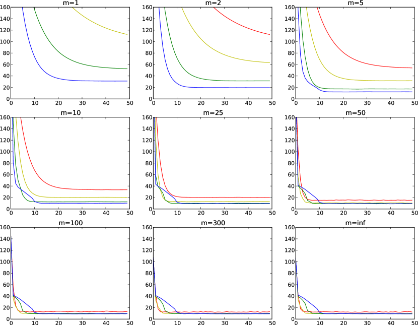
Figure 6: Average error of policy $\pi_{k,\ell}$ per iteration $k$ of MPI. Red lines for $\ell=1$, yellow for $\ell=2$, green for $\ell=5$ and blue for $\ell=10$.

In this last section, we describe an empirical illustration of our new variation of MPI on the dynamic location problem from Bertsekas and Yu (2012). The problem involves a repairman moving between $n$ sites according to some transition probabilities. As to allow him do his work, a trailer containing supplies for the repair jobs can be relocated to any of the sites at each decision epoch. The problem consists in finding a relocation policy for the trailer according the repairman’s and trailer’s positions which maximizes the discounted expectation of a reward function.

Given $n$ sites, the state space has $n^{2}$ states comprising the locations of both the repairman and the trailer. There are $n$ actions, each one corresponds to a possible destination of the trailer. Given an action $a=1,\dots,n$, and a state $s=(s_{r},s_{t})$, where the repairman and the trailer are at locations $s_{r}$ and $s_{t}$, respectively, we define the reward as $r(s,a)=-{\left\lvert s_{r}-s_{t}\right\rvert}-{\left\lvert s_{t}-a\right\rvert}/2$. At any time-step the repairman moves from its location $s_{r}<n$ with uniform probability to any location $s_{r}\leq s_{r}^{\prime}\leq n$; when $s_{r}=n$, he moves to site $1$ with probability $0.75$ or otherwise stays. Since the trailer moves are deterministic, the transition function is

$$T((s_{r},s_{t}),a,(s_{r}^{\prime},a))=\left\{\begin{array}[]{ll}\frac{1}{n-s_{r}+1}&\text{if }s_{r}<n\\ 0.75&\text{if }s_{r}=n\land s_{r}^{\prime}=1\\ 0.25&\text{if }s_{r}=n\land s_{r}^{\prime}=n\\ \end{array}\right.$$

and $0$ everywhere else.

We evaluated the empirical performance gain of using non-stationary policies by implementing the algorithm using random error vectors $\epsilon_{k}$, with each component being uniformly random between $0$ and some user-supplied value $\epsilon$. The adjustable size (with $n$) of the state and actions spaces allowed to compute an optimal policy to compare with the approximate ones generated by MPI for all combinations of parameters $\ell\in\{1,2,5,10\}$ and $m\in\{1,2,5,10,25,\infty\}$. Recall that the cases $m=1$ and $m=\infty$ correspond respectively to the non-stationary variants of VI and PI of Scherrer and Lesner (2012), while the case $\ell=1$ corresponds to the standard MPI algorithm. We used $n=8$ locations, $\gamma=0.98$ and $\epsilon=4$ in all experiments.

Figure 6 shows the average value of the error $v_{*}-v_{\pi_{k,\ell}}$ per iteration for the different values of parameters $m$ and $\ell$. For each parameter combination, the results are obtained by averaging over 250 runs. While higher values of $\ell$ impacts computational efficiency (by a factor $O(\ell)$) it always results with better performance. Especially with the lower values of $m$, a higher $\ell$ allows for faster convergence. While increasing $m$, this trend fades to be finally reversed in favor of faster convergence for small $\ell$. However, while small $\ell$ converges faster, it is with greater error than with higher $\ell$ after convergence. It can be seen that convergence is attained shortly after the $\ell^{\mathit{th}}$ iteration which can be explained by the fact that the first policies (involving $\pi_{0},\pi_{-1},\dots,\pi_{-\ell+2}$), are of poor quality and the algorithm must perform at least $\ell$ iterations to “push them out” of $\pi_{k,\ell}$.

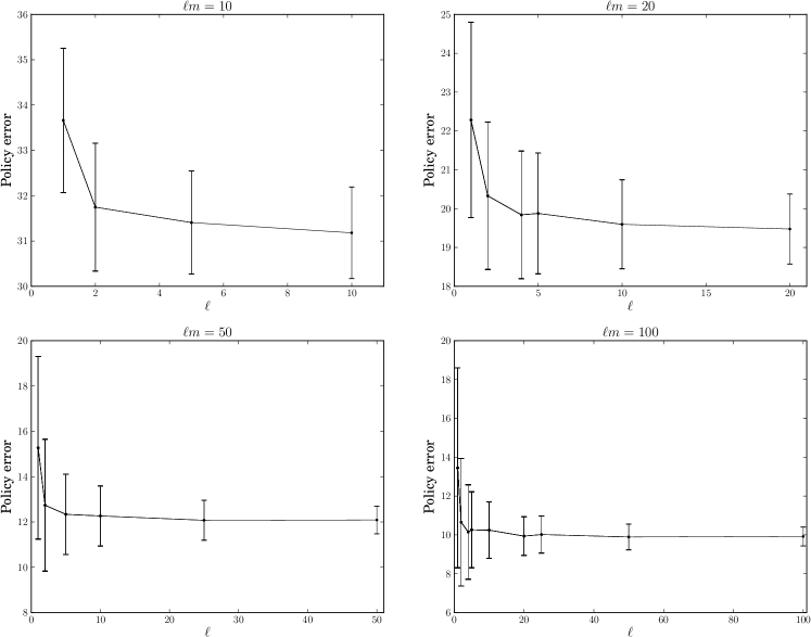
Figure 7: Policy error and standard deviation after $150$ iterations for different different values of $\ell$. Each plot represents a fixed value of the product $\ell m$. Data is collected over $250$ runs with $n=8$.

We conducted a second experiment to study the relative influence of the parameters $\ell$ and $m$. From the observation that the time complexity of an iteration of MPI can be roughly summarized by the number $\ell m+1$ of applications of a stationary policy’s Bellman operator, we ran the algorithm for fixed values of the product $\ell m$ and measured the policy error for varying values of $\ell$ after $150$ iterations. These results are depicted on Figure 7. This setting gives insight on how to set both parameters for a given “time budget” $\ell m$. While runs with a lower $\ell$ are slightly faster to converge, higher values always give the best policies after a sufficient number of iterations. It appears that favoring $\ell$ instead of $m$ seems to always be a good approach since it also greatly reduces the variance across all runs, showing that non-stationarity adds robustness to the approximation noise.

References

- Antos et al. (2007a) Antos, A., Munos, R., Szepesvari, C., et al. (2007a). Fitted Q-iteration in continuous action-space MDPs.
- Antos et al. (2007b) Antos, A., Szepesvarf, C., and Munos, R. (2007b). Value-iteration based fitted policy iteration: learning with a single trajectory. In Approximate Dynamic Programming and Reinforcement Learning, 2007. ADPRL 2007, pages 330–337. IEEE.
- Bertsekas and Tsitsiklis (1996) Bertsekas, D. and Tsitsiklis, J. (1996). Neuro-dynamic programming. Athena Scientific.
- Bertsekas and Yu (2012) Bertsekas, D. and Yu, H. (2012). Q-learning and enhanced policy iteration in discounted dynamic programming. Mathematics of Operations Research, 37(1), 66–94.
- Canbolat and Rothblum (2012) Canbolat, P. and Rothblum, U. (2012). (Approximate) iterated successive approximations algorithm for sequential decision processes. Annals of Operations Research, pages 1–12.
- Farahmand et al. (2010) Farahmand, A., Munos, R., and Szepesvári, C. (2010). Error propagation for approximate policy and value iteration (extended version). In NIPS.
- Kakade (2003) Kakade, S. (2003). On the Sample Complexity of Reinforcement Learning. Ph.D. thesis, University College London.
- Munos (2003) Munos, R. (2003). Error bounds for approximate policy iteration. In International Conference on Machine Learning (ICML), pages 560–567.
- Munos (2007) Munos, R. (2007). Performance bounds in -norm for approximate value iteration. SIAM Journal on Control and Optimization, 46(2), 541–561.
- Puterman (1994) Puterman, M. (1994). Markov decision processes: Discrete stochastic dynamic programming. John Wiley & Sons, Inc.
- Puterman and Shin (1978) Puterman, M. and Shin, M. (1978). Modified policy iteration algorithms for discounted Markov decision problems. Management Science, 24(11), 1127–1137.
- Scherrer and Lesner (2012) Scherrer, B. and Lesner, B. (2012). On the use of non-stationary policies for stationary infinite-horizon markov decision processes. In Advances in Neural Information Processing Systems 25, pages 1835–1843.
- Scherrer and Thiery (2010) Scherrer, B. and Thiery, C. (2010). Performance bound for approximate optimistic policy iteration. Technical report, INRIA.
- Scherrer et al. (2012a) Scherrer, B., Ghavamzadeh, M., Gabillon, V., and Geist, M. (2012a). Approximate modified policy iteration. In Proceedings of the 29th International Conference on Machine Learning (ICML-12), pages 1207–1214.
- Scherrer et al. (2012b) Scherrer, B., Gabillon, V., Ghavamzadeh, M., and Geist, M. (2012b). Approximate modified policy iteration. Technical report, INRIA.
- Singh and Yee (1994) Singh, S. and Yee, R. (1994). An upper bound on the loss from approximate optimal-value functions. Machine Learning, 16-3, 227–233.