Frequency-Domain Group-based Shrinkage Estimators for UWB Systems

Abstract

In this work, we propose low-complexity adaptive biased estimation algorithms, called group-based shrinkage estimators (GSEs), for parameter estimation and interference suppression scenarios with mechanisms to automatically adjust the shrinkage factors. The proposed estimation algorithms divide the target parameter vector into a number of groups and adaptively calculate one shrinkage factor for each group. GSE schemes improve the performance of the conventional least squares (LS) estimator in terms of the mean-squared error (MSE), while requiring a very modest increase in complexity. An MSE analysis is presented which indicates the lower bounds of the GSE schemes with different group sizes. We prove that our proposed schemes outperform the biased estimation with only one shrinkage factor and the best performance of GSE can be obtained with the maximum number of groups. Then, we consider an application of the proposed algorithms to single-carrier frequency-domain equalization (SC-FDE) of direct-sequence ultra-wideband (DS-UWB) systems, in which the structured channel estimation (SCE) algorithm and the frequency domain receiver employ the GSE. The simulation results show that the proposed algorithms significantly outperform the conventional unbiased estimator in the analyzed scenarios.

Index Terms–DS-UWB systems, parameter estimation, interference suppression, biased estimation, adaptive algorithm.

I Introduction

In this work, biased estimation algorithms are considered in two common deterministic estimation scenarios in communications engineering, which are parameter estimation and interference suppression [1]-[5]. It is known that under the assumption of AWGN, the least-square (LS) algorithm can provide an efficient solution to these estimation problems and will lead to minimum variance unbiased estimators (MVUE). The unbiasness is usually considered as a good property for an estimator because the expected value of unbiased estimators is the true value of the unknown parameter [6]. However, in some scenarios the LS method is not directly related to the mean square error (MSE) associated with the target parameter vector and it has been found that a lower MSE can be achieved by adding an appropriately chosen bias to the conventional LS estimators [7],[31]. Note that some reduced-rank techniques also employ a bias to accelerate the convergence speed [32]-[35].

A class of biased estimator that has been studied in recent years is known as the biased estimators with a shrinkage factor [7]-[14]. These biased estimation algorithms have shown their ability to outperform the existing unbiased estimators especially in low signal-to-noise ratios (SNR) scenarios and/or with short data records [9]. For these biased estimators [7]-[14], the complexity is much lower than for MMSE algorithms because the additional number of coefficients to be computed is only one. The motivation for the group-based shrinkage estimator (GSE) is to find a generalized estimator with a number of shrinkage factors that can achieve a better performance and complexity tradeoff than the biased estimator with only one shrinkage factor.

In the parameter estimation scenario,some biased estimators have been proposed to achieve a smaller estimation error than the LS solutions by removing the unbiasedness of the conventional estimators with a shrinkage factor in the parameter estimation scenario. The earliest shrinkage estimators that reduce the MSE over MVUE include the well known James-Stein estimator [10] and the work of Thompson [11]. Some extensions of the James-Stein estimator have been proposed in [12]-[15]. In [16], blind minimax estimation (BME) techniques have been proposed, in which the biased estimators were developed to minimize the worst case MSE among all possible values of the target parameter vector within a parameter set. If a spherical parameter set is assumed, the shrinkage estimator obtained is named spherical BME (SBME) [16].

For the interference suppression scenario, the biased estimators can be employed to achieve a lower estimation error between the estimated filter and the optimal linear LS estimator. The major motivation for adopting the biased algorithms here is to accelerate the convergence rate for the adaptive implementations and provide a better performance with short training data support in long filter scenarios [13].

To the best of our knowledge, biased estimators with shrinkage factors are rarely implemented into real-world signal processing and have not been considered in the frequency domain for communication systems. One possible reason is that some assumptions required for the signal model may not be satisfied. For example, in time-hopping UWB (TH-UWB) systems, the multiple access interference (MAI) cannot be accurately approximated by a Gaussian distribution for some values of the the signal-to-interference-plus-noise ratio (SINR) [17]. Another possible reason is that the existing shrinkage-based estimators usually require some statistical information such as the noise variance and the norm of the actual parameter vector. In our previous work [13] and [14], adaptive biased estimation algorithms with only one shrinkage factor have been proposed to fulfill the tasks of interference suppression and parameter estimation. In this work, a novel biased estimation technique, named group-based shrinkage estimators (GSE), is proposed. In this algorithm, the target parameter vector is divided into several groups and one shrinkage factor is calculated for each group. Least mean square (LMS)-based adaptive estimation algorithms are then developed to calculate the shrinkage factors. The GSE estimators are able to improve the performance of the recursive least squares (RLS) algorithm that recursively computes the LS estimator. In DS-UWB systems, the estimation tasks are usually very challenging because the environments include dense multipath. In this work, in order to test the proposed algorithms, we consider applications of DS-UWB systems with SC-FDE. Specifically, we concentrate on the channel estimation and interference suppression with the proposed algorithms. The MSE performance of the proposed GSE schemes is then analyzed, a lower bound of the MSE performance is derived and the relationship between the number of groups and the lower bound is set up. Simulations show that with an additional complexity that is only linearly dependent on the size of the parameter vector and the number of groups, the proposed biased GSE algorithms outperform the conventional RLS algorithm in terms of MSE in low SNR scenarios and/or with short data support. It should be noted that the proposed GSE estimator can be employed for applications where a high estimation accuracy is required. These include localization in wireless sensor networks [28] and in dense cluttered environments with UWB technology [29]. The proposed estimators can also be employed into emergent multicast and broadcast systems [5], such as the orthogonal frequency-division multiplexing (OFDM) based multi-user multiple-input multiple-output (MIMO) systems as specified in the IEEE 802.11ac standard and the 3GPP long-term-evolution (LTE) systems.

The main contributions of this work are summarized as follows:

• Novel GSE schemes are proposed to improve the performance of the frequency domain RLS algorithms in the applications of parameter estimation and interference suppression in DS-UWB systems.

• LMS based adaptive algorithms are developed for both scenarios to adjust the shrinkage factors.

• The MSE analysis is carried out which indicates a lower bound of the proposed estimator and the relationship between the lower bound and the number of groups.

• The performance of the proposed biased estimators is examined in multiuser SC-FDE for DS-UWB systems with the IEEE 802.15.4a channel model, convolutional and low-density parity-check (LDPC) codes.

The rest of this paper is structured as follows. In Section II, we first review the LS solution for the parameter estimation scenario and present the structured channel estimation (SCE) problem in SC-FDE of DS-UWB systems. Then, the signal model of the frequency domain receiver design for DS-UWB systems that represents the interference suppression scenario, is presented. The proposed GSE scheme and its adaptive implementations for the parameter estimation scenario and the interference suppression scenario are developed in Section III and Section IV, respectively. The MSE analysis is shown in Section V. The simulation results are shown in Section VI. Section VII draws the conclusions.

II System model

In this section, we introduce the channel estimation and receiver design tasks in the frequency-domain of DS-UWB systems with SC-FDE that represent the parameter estimation scenario and the interference suppression scenario, respectively.

II-A Problem statement for the parameter estimation scenario

The linear model for the parameter estimation scenario can be expressed as:

$$\mbox{\boldmath{$y$}}=\mbox{\boldmath{$X$}}\mbox{\boldmath{$h$}}+\mbox{\boldmath{$n$}},$$ (1)

where the training data matrix $\mbox{\boldmath{$X$}}\in\mathbb{C}^{M\times L}$ and the received signal $\mbox{\boldmath{$y$}}\in\mathbb{C}^{M\times 1}$ are given, $n$ is AWGN with zero mean and variance $\sigma^{2}$. In this scenario, the typical target is to estimate the parameter vector $\mbox{\boldmath{$h$}}\in\mathbb{C}^{L\times 1}$ that leads to the minimum MSE. The MSE consists of the estimation variance and the squared bias and is given by

$${\mathbb{E}}\{\|\mbox{\boldmath{$h$}}-\hat{\mbox{\boldmath{$h$}}}\|^{2}\}={\mathbb{E}}\{(\hat{\mbox{\boldmath{$h$}}}-{\mathbb{E}}\{\hat{\mbox{\boldmath{$h$}}}\})^{H}(\hat{\mbox{\boldmath{$h$}}}-{\mathbb{E}}\{\hat{\mbox{\boldmath{$h$}}}\})\}+[\|{\mathbb{E}}\{\hat{\mbox{\boldmath{$h$}}}\}-\mbox{\boldmath{$h$}}\|^{2}],$$

where ${\mathbb{E}}\{\cdot\}$ represents expectation of a random variable.

The conventional LS algorithm estimates the parameter by minimizing

$${J}_{\rm LS}(\mbox{\boldmath{$h$}})=\|\mbox{\boldmath{$y$}}-\mbox{\boldmath{$X$}}\mbox{\boldmath{$h$}}\|^{2}.$$ (2)

Assuming that the matrix $\mbox{\boldmath{$X$}}^{H}\mbox{\boldmath{$X$}}$ is a full rank matrix, the LS solution is given by

$$\hat{\mbox{\boldmath{$h$}}}_{\rm LS}=(\mbox{\boldmath{$X$}}^{H}\mbox{\boldmath{$X$}})^{-1}\mbox{\boldmath{$X$}}^{H}\mbox{\boldmath{$y$}}.$$ (3)

Under the assumption of AWGN with zero mean and variance $\sigma^{2}$, the LS estimator is a MVUE that leads to a minimum MSE

$${\mathbb{E}}\{\|\mbox{\boldmath{$h$}}-\hat{\mbox{\boldmath{$h$}}}_{\rm LS}\|^{2}\}={\mathbb{E}}\{(\hat{\mbox{\boldmath{$h$}}}_{\rm LS}-\mbox{\boldmath{$h$}})^{H}(\hat{\mbox{\boldmath{$h$}}}_{\rm LS}-\mbox{\boldmath{$h$}})\}=var(\mbox{\boldmath{$h$}},\hat{\mbox{\boldmath{$h$}}}_{\rm LS}).$$

we define $v=var(\mbox{\boldmath{$h$}},\hat{\mbox{\boldmath{$h$}}}_{\rm LS})=tr\{\sigma^{2}(\mbox{\boldmath{$X$}}^{H}\mbox{\boldmath{$X$}})^{-1}\}$, where $tr\{\cdot\}$ represents the trace operator [6].

The objective of introducing the biased estimator in the parameter estimation scenario is to achieve a lower MSE than the unbiased estimator, which can be expressed as

$${\mathbb{E}}\{\|\mbox{\boldmath{$h$}}-\hat{\mbox{\boldmath{$h$}}}_{\rm b}\|^{2}\}\leq{\mathbb{E}}\{\|\mbox{\boldmath{$h$}}-\hat{\mbox{\boldmath{$h$}}}_{\rm LS}\|^{2}\}.$$ (4)

Although the objective shown here is similar to MMSE algorithms that is to achieve an MSE as small as possible. It should be noted that the biased algorithm developed in this work adopts a different strategy from MMSE algorithms.

II-B System model for the SCE: parameter estimation scenario

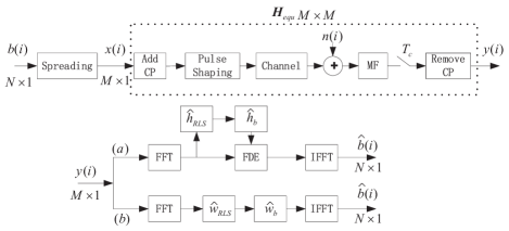
Figure 1: Block diagram of SC-FDE schemes in DS-UWB systems: (a) Parameter estimation scenario,(b) Interference suppression scenario.

Here, we consider the channel estimation problem of a synchronous downlink block-by-block transmission DS-UWB system based on SC-FDE with $K$ users. The block diagram of the parameter estimation scenario is shown as branch (a) in Fig. 1. For notational simplicity, we assume that a $N_{c}$-by-$1$ Walsh spreading code $\mbox{\boldmath{$s$}}_{k}$ is assigned to the $k$-th user. The spreading gain is $N_{c}=T_{s}/T_{c}$, where $T_{s}$ and $T_{c}$ denote the symbol duration and chip duration, respectively. At each time instant $i$, a data vector $\mbox{\boldmath{$b$}}_{k}(i)\in\mathbb{C}^{N\times 1}$ is transmitted by the $k$-th user. We define the signal after spreading as $\mbox{\boldmath{$x$}}_{k}(i)=\mbox{\boldmath{$D$}}_{k}\mbox{\boldmath{$b$}}_{k}(i)$, where the block diagonal matrix $\mbox{\boldmath{$D$}}_{k}\in\mathbb{C}^{M\times N}$ ($M=N\cdot N_{c}$) performs the spreading of the data block and its first column is constructed by the spreading code $\mbox{\boldmath{$s$}}_{k}$ zero-padded to the length of $M$. In order to prevent inter block interference (IBI), a cyclic-prefix (CP) is added and the length of the CP is assumed to be larger than the length of the channel impulse response (CIR). With the insertion of the CP at the transmitter and its removal at the receiver, the equivalent channel is denoted as a circulant Toeplitz matrix $\mbox{\boldmath{$H$}}_{\rm equ}\in\mathbb{C}^{M\times M}$, whose first column is composed of a vector $\mbox{\boldmath{$h$}}_{\rm equ}$ zero-padded to length $M$, where $\mbox{\boldmath{$h$}}_{\rm equ}=[h(0),h(1),\dots,h(L-1)]$ is the equivalent CIR. At the receiver, a chip matched-filter (CMF) is applied and the received sequence is then sampled at chip-rate and organized in an $M$-dimensional vector. This signal then goes through the discrete Fourier transform (DFT). The frequency-domain received signal is given by

$$\mbox{\boldmath{$y$}}(i)=\mbox{\boldmath{$F$}}\mbox{\boldmath{$H$}}_{\rm equ}\sum_{k=1}^{K}\mbox{\boldmath{$x$}}_{k}(i)+\mbox{\boldmath{$F$}}\mbox{\boldmath{$n$}}(i)=\mbox{\boldmath{$\Lambda$}}_{\rm H}\mbox{\boldmath{$F$}}\sum_{k=1}^{K}\mbox{\boldmath{$x$}}_{k}(i)+\mbox{\boldmath{$F$}}\mbox{\boldmath{$n$}}(i),$$ (5)

where $\mbox{\boldmath{$n$}}(i)$ represents the AWGN, $\mbox{\boldmath{$\Lambda$}}_{\rm H}=\mbox{\boldmath{$F$}}\mbox{\boldmath{$H$}}_{\rm equ}\mbox{\boldmath{$F$}}^{H}$ is a diagonal matrix whose diagonal vector is defined as $\tilde{\mbox{\boldmath{$h$}}}$ and its $a$-th entry is given by $\tilde{h}_{a}=\sum_{l=0}^{L-1}h_{l}\cdot{\rm exp}\{-j(2\pi/M)a\hskip 1.49994ptl\}$, where $a$ $\in$ $\{0,1,2,\dots,M-1\}$. $\mbox{\boldmath{$F$}}\in\mathbb{C}^{M\times M}$ represents the DFT matrix and its $(a,b)$-th entry is ${\mbox{\boldmath{$F$}}}_{a,b}$$=(1/\sqrt{M}){\rm exp}\{-j(2\pi/M)a\hskip 1.49994ptb\},$ where $a,b$ $\in$ $\{0,1,2,\dots,M-1\}$. By defining a matrix $\mbox{\boldmath{$F$}}_{M,L}\in\mathbb{C}^{M\times L}$ that contains the first $L$ columns of the DFT matrix $F$, we obtain the following relationship

$$\tilde{\mbox{\boldmath{$h$}}}=\sqrt{M}\mbox{\boldmath{$F$}}_{M,L}\mbox{\boldmath{$h$}}_{\rm equ},$$ (6)

In unstructured channel estimation (UCE), the vector $\tilde{\mbox{\boldmath{$h$}}}\in\mathbb{C}^{M\times 1}$ is directly estimated, while in the structured channel estimation (SCE), the fact that $L<M$ is taken into account and the vector $\mbox{\boldmath{$h$}}_{\rm equ}\in\mathbb{C}^{L\times 1}$ is the parameter vector to be estimated. The concept of SCE was proposed in [20], where the SCE shows a better performance than the UCE. In [21], adaptive MMSE detection schemes for SC-FDE in multi-user DS-UWB systems based on SCE are developed, where the estimated $\mbox{\boldmath{$h$}}_{\rm equ}$ is adaptively calculated based on RLS, least-mean squares (LMS) and the conjugate gradient (CG) algorithm for the detection and the RLS version performs the best. The purpose of developing biased estimation in this scenario is to further improve the performance of the RLS algorithm in terms of the MSE.

We consider user 1 as the desired user and omit the subscript of this user for simplicity. Note that the frequency domain received signal can be expressed as

$$\mbox{\boldmath{$y$}}(i)=\sqrt{M}\mbox{\boldmath{$\Delta$}}(i)\mbox{\boldmath{$F$}}_{M,L}\mbox{\boldmath{$h$}}_{\rm equ}+\mbox{\boldmath{$n$}}_{\rm e}(i),$$ (7)

where we define a diagonal matrix $\mbox{\boldmath{$\Delta$}}(i)={\rm diag}[\mbox{\boldmath{$F$}}\mbox{\boldmath{$x$}}(i)]$, the noise and interference vector $\mbox{\boldmath{$n$}}_{\rm e}(i)$ consists of the MAI and the noise and is assumed to be AWGN. As shown in (7), the SCE problem is an implementation example of the parameter estimation problem where a given matrix $\mbox{\boldmath{$X$}}(i)\in\mathbb{C}^{M\times L}$ is defined as $\mbox{\boldmath{$X$}}(i)=\sqrt{M}\mbox{\boldmath{$\Delta$}}(i)\mbox{\boldmath{$F$}}_{M,L}$. The LS solution of $\mbox{\boldmath{$h$}}_{\rm equ}$ is given by

$${\mbox{\boldmath{$h$}}}_{\rm equ,LS}(i)=\mbox{\boldmath{$R$}}_{\rm h}^{-1}(i)\mbox{\boldmath{$p$}}_{\rm h}(i)$$ (8)

where $\mbox{\boldmath{$R$}}_{\rm h}(i)=\sum_{j=1}^{i}\lambda^{i-j}\mbox{\boldmath{$F$}}^{H}_{M,L}\mbox{\boldmath{$\Delta$}}^{H}(j)\mbox{\boldmath{$\Delta$}}(j)\mbox{\boldmath{$F$}}_{M,L}$, $\mbox{\boldmath{$p$}}_{\rm h}(i)=\sum_{j=1}^{i}\lambda^{i-j}\mbox{\boldmath{$F$}}^{H}_{M,L}\mbox{\boldmath{$\Delta$}}^{H}(j)\mbox{\boldmath{$z$}}(j)$ and $\lambda$ is the forgetting factor. Then the LS solution can be computed recursively by the following RLS algorithm [20]

$$\hat{\mbox{\boldmath{$h$}}}_{\rm RLS}(i+1)=\hat{\mbox{\boldmath{$h$}}}_{\rm RLS}(i)+\mbox{\boldmath{$R$}}_{\rm h}^{-1}(i)\mbox{\boldmath{$F$}}^{H}_{M,L}\mbox{\boldmath{$\Delta$}}^{H}(i)\mbox{\boldmath{$e$}}_{\rm h}(i),$$ (9)

where $\mbox{\boldmath{$e$}}_{\rm h}(i)=\mbox{\boldmath{$z$}}(i)-\mbox{\boldmath{$\Delta$}}(i)\mbox{\boldmath{$F$}}_{M,L}\hat{\mbox{\boldmath{$h$}}}_{\rm RLS}(i)$ is the $M$-dimensional error vector.

In Section III, a novel biased estimation algorithm called group-based shrinkage estimator (GSE) is incorporated into the unbiased LS estimator that is able to improve the estimation performance in terms of the MSE.

II-C System model for the frequency domain receiver design: interference suppression scenario

The block diagram of the interference suppression scenario is shown as branch (b) in Fig. 1. For each time instant $i$, an $N$-dimensional data vector $\mbox{\boldmath{$b$}}_{k}(i)=[b_{k}^{(1)}(i),\dots,b_{k}^{(N)}(i)]^{T}$ is transmitted by the $k$-th user. After the spreading, the $M$-dimensional transmit signal is given by

$$\mbox{\boldmath{$x$}}_{k}(i)=\mbox{\boldmath{$S$}}_{k}\mbox{\boldmath{$b$}}_{k,{\rm e}}(i),$$ (10)

where the spreading matrix $\mbox{\boldmath{$S$}}_{k}\in\mathbb{C}^{M\times M}$, $M=N\times N_{c}$, is a circulant Toeplitz matrix and its first column consists of the spreading codes and zero-padding [26]. The equivalent $M$-dimensional expanded data vector is

$$\mbox{\boldmath{$b$}}_{k,{\rm e}}(i)=[b_{k}^{(1)}(i),\mbox{\boldmath{$0$}}_{N_{c}-1},b_{k}^{(2)}(i),\mbox{\boldmath{$0$}}_{N_{c}-1},\cdots,b_{k}^{(N)}(i),\mbox{\boldmath{$0$}}_{N_{c}-1}]^{T},$$

where $(\cdot)^{T}$ is the transpose. Using this signal expression we can obtain a simplified frequency domain receiver design. At the receiver, a CMF is applied and the received sequence is then sampled at chip-rate and organized in an $M$-dimensional vector. After the DFT, the received signal is given by

$$\mbox{\boldmath{$z$}}(i)=\mbox{\boldmath{$F$}}\mbox{\boldmath{$y$}}(i)=\sum_{k=1}^{K}\mbox{\boldmath{$F$}}\mbox{\boldmath{$H$}}_{\rm equ}\mbox{\boldmath{$S$}}_{k}\mbox{\boldmath{$b$}}_{k,{\rm e}}(i)+\mbox{\boldmath{$F$}}\mbox{\boldmath{$n$}}(i),$$ (11)

where $\mbox{\boldmath{$n$}}(i)$ is the AWGN and $\mbox{\boldmath{$F$}}\in\mathbb{C}^{M\times M}$ represents the DFT matrix. Since both $\mbox{\boldmath{$H$}}_{\rm equ}$ and $\mbox{\boldmath{$S$}}_{k}$ are circulant Toeplitz matrices, their product also has the circulant Toeplitz form. This feature makes $\mbox{\boldmath{$\Lambda$}}_{k}=\mbox{\boldmath{$F$}}\mbox{\boldmath{$H$}}_{\rm equ}\mbox{\boldmath{$S$}}_{k}\mbox{\boldmath{$F$}}^{H}$ a diagonal matrix. Hence, we have

$$\mbox{\boldmath{$z$}}(i)=\sum_{k=1}^{K}\mbox{\boldmath{$\Lambda$}}_{k}\mbox{\boldmath{$F$}}\mbox{\boldmath{$b$}}_{k,{\rm e}}(i)+\mbox{\boldmath{$F$}}\mbox{\boldmath{$n$}}(i).$$ (12)

We can further expand $\mbox{\boldmath{$F$}}\mbox{\boldmath{$b$}}_{k,{\rm e}}(i)$ as [26]

$$\mbox{\boldmath{$F$}}\mbox{\boldmath{$b$}}_{k,{\rm e}}(i)=(1/\sqrt{N_{c}})\mbox{\boldmath{$I$}}_{\rm e}\mbox{\boldmath{$F$}}_{N}\mbox{\boldmath{$b$}}_{k}(i),$$ (13)

where $\mbox{\boldmath{$F$}}_{N}\in\mathbb{C}^{N\times N}$ denotes the DFT matrix and $\mbox{\boldmath{$I$}}_{\rm e}\in\mathbb{C}^{M\times N}$ is structured as

$$\mbox{\boldmath{$I$}}_{\rm e}=[\underbrace{\mbox{\boldmath{$I$}}_{N},\cdots,\mbox{\boldmath{$I$}}_{N}}_{N_{c}}]^{T}.$$ (14)

where $\mbox{\boldmath{$I$}}_{N}$ denotes the $N$-by-$N$ identity matrix. Finally, the frequency domain received signal $\mbox{\boldmath{$z$}}(i)$ is given by

$$\mbox{\boldmath{$z$}}(i)=\sum_{k=1}^{K}(1/\sqrt{N_{c}})\mbox{\boldmath{$\Lambda$}}_{k}\mbox{\boldmath{$I$}}_{\rm e}\mbox{\boldmath{$F$}}_{N}\mbox{\boldmath{$b$}}_{k}(i)+\mbox{\boldmath{$F$}}\mbox{\boldmath{$n$}}(i).$$ (15)

Note that the expression in (15) is an implementation example of the interference suppression scenario where the unknown matrix for each time instant is given by $\mbox{\boldmath{$H$}}(i)=(1/\sqrt{N_{c}})\mbox{\boldmath{$\Lambda$}}_{k}\mbox{\boldmath{$I$}}_{\rm e}\mbox{\boldmath{$F$}}_{N}$. To fulfill the interference suppression task, an MMSE filter $\mbox{\boldmath{$W$}}(i)\in\mathbb{C}^{M\times N}$ can be developed via the following cost function:

$${J}_{\rm MSE}(i)={\mathbb{E}}\big{\{}\left\|\mbox{\boldmath{$b$}}(i)-\mbox{\boldmath{$F$}}_{N}^{H}\mbox{\boldmath{$W$}}^{H}(i)\mbox{\boldmath{$z$}}(i)\right\|^{2}\big{\}}.$$ (16)

The MMSE solution is given by [21]

$$\mbox{\boldmath{$W$}}_{\rm MMSE}=\mbox{\boldmath{$V$}}\mbox{\boldmath{$I$}}_{\rm e},$$ (17)

where the matrix $\mbox{\boldmath{$V$}}\in\mathbb{C}^{M\times M}$ is

$$\mbox{\boldmath{$V$}}=\frac{1}{\sqrt{N_{c}}}\left(\frac{1}{N_{c}}\sum_{k=1}^{K}\mbox{\boldmath{$\Lambda$}}_{k}\mbox{\boldmath{$I$}}_{\rm e}\mbox{\boldmath{$I$}}_{\rm e}^{H}\mbox{\boldmath{$\Lambda$}}_{k}^{H}+\sigma^{2}\mbox{\boldmath{$I$}}_{M}\right)^{-1}\mbox{\boldmath{$\Lambda$}}_{k},$$ (18)

where $\mbox{\boldmath{$I$}}_{M}\in\mathbb{C}^{M\times M}$ denotes the identity matrix. Note that the matrix $V$ consists of $N_{c}$ times $N_{c}$ diagonal matrices $\mbox{\boldmath{$V$}}_{ij}\in\mathbb{C}^{N\times N}$, where $i,j$ $\in$ $\{1,N_{c}\}$. Hence, we take a closer look at the product of $V$ and $\mbox{\boldmath{$I$}}_{\rm e}$:

$$\begin{split}&\mbox{\boldmath{$V$}}\mbox{\boldmath{$I$}}_{e}=\begin{bmatrix}\mbox{\boldmath{$V$}}_{1,1}&\mbox{\boldmath{$V$}}_{1,2}&\dots&\mbox{\boldmath{$V$}}_{1,N_{c}}\\ \mbox{\boldmath{$V$}}_{2,1}&\mbox{\boldmath{$V$}}_{2,2}&\dots&\mbox{\boldmath{$V$}}_{2,N_{c}}\\ \vdots&\vdots&\vdots&\vdots\\ \mbox{\boldmath{$V$}}_{N_{c},1}&\mbox{\boldmath{$V$}}_{N_{c},2}&\dots&\mbox{\boldmath{$V$}}_{N_{c},N_{c}}\\ \end{bmatrix}\begin{bmatrix}\mbox{\boldmath{$I$}}_{N}\\ \mbox{\boldmath{$I$}}_{N}\\ \vdots\\ \mbox{\boldmath{$I$}}_{N}\\ \end{bmatrix}\\ &=\begin{bmatrix}\sum_{j=1}^{N_{c}}\mbox{\boldmath{$V$}}_{1,j}\\ \sum_{j=1}^{N_{c}}\mbox{\boldmath{$V$}}_{2,j}\\ \vdots\\ \sum_{j=1}^{N_{c}}\mbox{\boldmath{$V$}}_{N_{c},j}\\ \end{bmatrix}=\begin{bmatrix}\hat{\mbox{\boldmath{$W$}}}_{1}&&&\\ &\hat{\mbox{\boldmath{$W$}}}_{2}&&\\ &&\ddots&\\ &&&\hat{\mbox{\boldmath{$W$}}}_{N_{c}}\\ \end{bmatrix}\begin{bmatrix}\mbox{\boldmath{$I$}}_{N}\\ \mbox{\boldmath{$I$}}_{N}\\ \vdots\\ \mbox{\boldmath{$I$}}_{N}\\ \end{bmatrix}=\hat{\mbox{\boldmath{$W$}}}\mbox{\boldmath{$I$}}_{\rm e},\end{split}$$

where $\hat{\mbox{\boldmath{$W$}}}_{i}=\sum_{j=1}^{N_{c}}\mbox{\boldmath{$V$}}_{i,j}$, $i=1,\dots,N_{c}$, are diagonal matrices. Hence, the product of $V$ and $\mbox{\boldmath{$I$}}_{\rm e}$ can be converted into a product of a diagonal matrix $\hat{\mbox{\boldmath{$W$}}}\in\mathbb{C}^{M\times M}$ ($M=N\times N_{c}$) and $\mbox{\boldmath{$I$}}_{\rm e}$, where the diagonal entries of $\hat{\mbox{\boldmath{$W$}}}$ are $\hat{w}_{l}$, $l=1,\dots,M$, and equal the sum of all entries in the $l$-th row of matrix $V$. Finally, we express the MMSE design as

$$\mbox{\boldmath{$W$}}_{\rm MMSE}=\hat{\mbox{\boldmath{$W$}}}\mbox{\boldmath{$I$}}_{\rm e}={\rm diag}(\hat{\mbox{\boldmath{$w$}}}_{\rm e})\mbox{\boldmath{$I$}}_{\rm e},$$ (19)

where $\hat{\mbox{\boldmath{$w$}}}_{\rm e}=(\hat{w}_{1},\hat{w}_{2},\dots,\hat{w}_{M})$ is an equivalent filter with $M$ taps.

The expression shown in (19) enables us to design an $M$-dimensional receive filter rather than an $M$-by-$N$ matrix form receive filter. The estimated data vector can be expressed as

$$\hat{\mbox{\boldmath{$b$}}}(i)=\mbox{\boldmath{$F$}}_{N}^{H}\mbox{\boldmath{$I$}}_{\rm e}^{H}\hat{\mbox{\boldmath{$W$}}}^{H}(i)\mbox{\boldmath{$z$}}(i)=\mbox{\boldmath{$F$}}_{N}^{H}\mbox{\boldmath{$I$}}_{\rm e}^{H}\hat{\mbox{\boldmath{$Z$}}}(i)\hat{\mbox{\boldmath{$w$}}}(i),$$ (20)

where $\hat{\mbox{\boldmath{$Z$}}}(i)={\rm diag}(\mbox{\boldmath{$z$}}(i))$ and $\hat{\mbox{\boldmath{$w$}}}(i)=\hat{\mbox{\boldmath{$w$}}}_{\rm e}^{*}(i)$ is the weight vector of the adaptive receiver. Since $\mbox{\boldmath{$F$}}_{N}$ and $\mbox{\boldmath{$I$}}_{\rm e}$ are fixed, we consider the equivalent $N$-by-$M$ received data matrix as $\mbox{\boldmath{$Y$}}(i)=\mbox{\boldmath{$F$}}_{N}^{H}\mbox{\boldmath{$I$}}_{\rm e}^{H}\hat{\mbox{\boldmath{$Z$}}}(i),$ and express the estimated data vector as $\hat{\mbox{\boldmath{$b$}}}(i)=\mbox{\boldmath{$Y$}}(i)\hat{\mbox{\boldmath{$w$}}}(i)$.

II-D LS solution and adaptive RLS algorithm for the interference suppression scenario

Here, we detail the LS and RLS designs for the frequency domain multiuser receiver $\hat{\mbox{\boldmath{$w$}}}$. The cost function for the development of the LS estimation is given by

$$J_{\rm LS}=\|\mbox{\boldmath{$b$}}-\mbox{\boldmath{$Y$}}\mbox{\boldmath{$w$}}\|^{2}.$$ (21)

The LS design of the linear receiver can be expressed as

$$\hat{\mbox{\boldmath{$w$}}}_{\rm LS}=(\mbox{\boldmath{$Y$}}^{H}\mbox{\boldmath{$Y$}})^{-1}\mbox{\boldmath{$Y$}}^{H}\mbox{\boldmath{$b$}}=\mbox{\boldmath{$R$}}_{\rm LS}^{-1}\mbox{\boldmath{$p$}}_{\rm LS},$$ (22)

where the matrix $\mbox{\boldmath{$R$}}_{\rm LS}$ is defined as $\mbox{\boldmath{$Y$}}^{H}\mbox{\boldmath{$Y$}}$ and $\mbox{\boldmath{$p$}}_{\rm LS}$ represents the vector $\mbox{\boldmath{$Y$}}^{H}\mbox{\boldmath{$b$}}$. Note that, the data vector can be expressed as

$$\mbox{\boldmath{$b$}}=\mbox{\boldmath{$Y$}}\mbox{\boldmath{$w$}}_{\rm o}+\mbox{\boldmath{$\epsilon$}}_{\rm o},$$ (23)

where $\mbox{\boldmath{$\epsilon$}}_{\rm o}$ is the measurement error vector and $\mbox{\boldmath{$w$}}_{\rm o}$ is the optimum tap-weight vector of the receiver (optimum in the MSE sense). Assuming that $\mbox{\boldmath{$\epsilon$}}_{\rm o}$ is white and Gaussian with zero mean and covariance of $\sigma_{e}^{2}\mbox{\boldmath{$I$}}_{N}$, then the LS solution in (22) is a MVUE [27]. Now, let us have a look at the following MSE:

$${\mathbb{E}}\{\|\mbox{\boldmath{$w$}}_{\rm o}-\hat{\mbox{\boldmath{$w$}}}_{\rm LS}\|^{2}\}={\mathbb{E}}\{(\mbox{\boldmath{$w$}}_{\rm o}-\hat{\mbox{\boldmath{$w$}}}_{\rm LS})^{H}(\mbox{\boldmath{$w$}}_{\rm o}-\hat{\mbox{\boldmath{$w$}}}_{\rm LS})\}=var(\mbox{\boldmath{$w$}}_{\rm o},\hat{\mbox{\boldmath{$w$}}}_{\rm LS}).$$ (24)

Defining $v_{w}=var(\mbox{\boldmath{$w$}}_{\rm o},\hat{\mbox{\boldmath{$w$}}}_{\rm LS})$, we have [6]

$$v_{w}=tr\{\sigma_{e}^{2}(\mbox{\boldmath{$Y$}}^{H}\mbox{\boldmath{$Y$}})^{-1}\},$$ (25)

where $\sigma_{e}^{2}$ is the variance of the measurement error.

In the interference suppression scenario, it is possible to introduce the biased estimation to reduce the MSE between the optimal receive filter $\mbox{\boldmath{$w$}}_{\rm o}$ and the LS estimator $\hat{\mbox{\boldmath{$w$}}}_{\rm LS}$. Note that, for the interference suppression scenario, the typical objective is to minimize the overall performance criterion which is determined as $\mathbb{E}\{\|\mbox{\boldmath{$b$}}-\hat{\mbox{\boldmath{$b$}}}\|^{2}\}$, rather than to minimize ${\mathbb{E}}\{\|\mbox{\boldmath{$w$}}_{\rm o}-\hat{\mbox{\boldmath{$w$}}}\|^{2}\}$. The main motivation to introduce the bias in the interference suppression scenario is to provide an initial improvement for the overall performance when the adaptive filtering techniques are employed and the training data are limited. This can also help with tracking problems and with robustness against interference.

The LS solution of the receiver can be computed recursively by the RLS adaptive algorithm. We employ the RLS update equation that is proposed in [21]

$$\hat{\mbox{\boldmath{$w$}}}_{\rm RLS}(i+1)=\hat{\mbox{\boldmath{$w$}}}_{\rm RLS}(i)+\mbox{\boldmath{$R$}}_{\rm w}^{-1}(i)\mbox{\boldmath{$Y$}}^{H}(i)\mbox{\boldmath{$e$}}_{\rm aw}(i),$$ (26)

where $\mbox{\boldmath{$R$}}_{\rm w}(i)=\sum_{j=1}^{i}\lambda_{w}^{i-j}\mbox{\boldmath{$Y$}}^{H}(j)\mbox{\boldmath{$Y$}}(j)$ and $\mbox{\boldmath{$e$}}_{\rm aw}(i)=\mbox{\boldmath{$b$}}(i)-\mbox{\boldmath{$Y$}}(i)\hat{\mbox{\boldmath{$w$}}}(i)$. Note that $\mbox{\boldmath{$R$}}_{\rm w}(i)$ is an $M$-by-$M$ symmetric sparse matrix in which the number of nonzero elements equals $MN_{c}$. Hence, the complexity of each adaptation by using this algorithm is $\mathcal{O}(MN_{c}^{2})$.

III Proposed GSE for parameter estimation scenario

III-A Proposed GSE: Optimal Solution

It is known that the biased estimator with a shrinkage factor can be expressed as

$$\hat{\mbox{\boldmath{$h$}}}_{\rm b}=(1+\alpha)\hat{\mbox{\boldmath{$h$}}}_{\rm LS},$$ (27)

where $\hat{\mbox{\boldmath{$h$}}}_{\rm LS}\in\mathbb{C}^{L\times 1}$ is the LS estimator of the parameter vector and $\hat{\mbox{\boldmath{$h$}}}_{\rm b}\in\mathbb{C}^{L\times 1}$ is the biased estimator with a shrinkage factor, $\alpha$ is a real-valued variable and $(1+\alpha)$ is defined as the real-valued shrinkage factor that is larger than 0 but smaller than 1 (i.e., $-1<\alpha<0$).

Actually, for the parameter estimation scenario, the MMSE estimators with the following expression can also be considered as a biased estimator,

$$\hat{\mbox{\boldmath{$h$}}}_{\rm MMSE}=\mbox{\boldmath{$A$}}\hat{\mbox{\boldmath{$h$}}}_{\rm LS},$$ (28)

where $\hat{\mbox{\boldmath{$h$}}}_{\rm MMSE}\in\mathbb{C}^{L\times 1}$ and $\mbox{\boldmath{$A$}}\in\mathbb{C}^{L\times L}$ is a full-rank matrix. As in [22] and [23], such MMSE channel estimators are developed for MIMO and OFDM systems, respectively. Although these MMSE estimators can achieve a much lower MSE than the LS estimator especially in low SNR regime, they experience much higher complexity than the biased estimator with only one shrinkage factor. In [22], the proposed scaled LS channel estimator can be considered as a biased estimator with only one shrinkage factor, which outperforms the conventional LS estimator while it requires a much lower complexity than the MMSE estimator. The basic idea of the following proposed group-based shrinkage estimator (GSE) is to find a solution with a better tradeoff between the complexity and the performance than the MMSE estimator and the biased estimator with only one shrinkage factor.

The proposed GSE can be expressed as follows:

$$\hat{\mbox{\boldmath{$h$}}}_{\rm b}=\begin{bmatrix}(1+\alpha_{1})\hat{h}_{\rm LS}(1)\\ \vdots\\ (1+\alpha_{1})\hat{h}_{\rm LS}(\frac{L}{S})\\ (1+\alpha_{2})\hat{h}_{\rm LS}(\frac{L}{S}+1)\\ \vdots\\ (1+\alpha_{2})\hat{h}_{\rm LS}(\frac{2L}{S})\\ \vdots\\ (1+\alpha_{S})\hat{h}_{\rm LS}(\frac{(S-1)L}{S}+1)\\ \vdots\\ (1+\alpha_{S})\hat{h}_{\rm LS}(L)\\ \end{bmatrix}=\hat{\mbox{\boldmath{$H$}}}_{\rm LS}({\bf 1}_{S}+\boldsymbol{\alpha})$$ (29)

where $\hat{\mbox{\boldmath{$H$}}}_{\rm LS}\in\mathbb{C}^{L\times S}$ is a block diagonal matrix that is constructed from the elements of $\hat{\mbox{\boldmath{$h$}}}_{\rm LS}$ as well as zeros, $S$ is the number of groups, we define the $S$-dimensional column vectors ${\bf 1}_{S}=[1,1,\dots,1]^{T}$ and $\boldsymbol{\alpha}=[\alpha_{1},\alpha_{2},\dots,\alpha_{S}]^{T}$. The scalar $\alpha_{s}$ is a real-valued variable and $(1+\alpha_{s})$ is defined as the shrinkage factor for the $s$-th group of coefficients that is larger than 0 but smaller than 1, where $s=1,2,\dots,S$. Here we propose to use a uniform group size for the $L$-dimensional parameter vector, hence the size of each group is $L/S$. If the length of the parameter vector divided by the group size is not an integer, we can perform zero-padding in the parameter estimation vector to fulfill this requirement. If any statistical knowledge of the parameter vector is given, the group size could be different from each other. But this approach will introduce a higher complexity because we need to select the size of each group and choose a suitable one. In this work, for notational simplicity, we will focus on the low complexity uniform group size approach.

The goal is to minimize the MSE defined by

$${\mathbb{E}}\{\|\mbox{\boldmath{$h$}}-\hat{\mbox{\boldmath{$h$}}}_{\rm b}\|^{2}\}={\mathbb{E}}\{(\hat{\mbox{\boldmath{$h$}}}_{\rm b}-{\mathbb{E}}\{\hat{\mbox{\boldmath{$h$}}}_{\rm b}\})^{H}(\hat{\mbox{\boldmath{$h$}}}_{\rm b}-{\mathbb{E}}\{\hat{\mbox{\boldmath{$h$}}}_{\rm b}\})\}+\|{\mathbb{E}}\{\hat{\mbox{\boldmath{$h$}}}_{\rm b}\}-\mbox{\boldmath{$h$}}\|^{2}.$$ (30)

Note that

$$\hat{\mbox{\boldmath{$h$}}}_{\rm b}-{\mathbb{E}}\{\hat{\mbox{\boldmath{$h$}}}_{\rm b}\}=(\hat{\mbox{\boldmath{$H$}}}_{\rm LS}-{\mbox{\boldmath{$H$}}})({\bf 1}_{S}+\boldsymbol{\alpha})$$ (31)

and we have $\hat{\mbox{\boldmath{$H$}}}_{\rm LS}={\mbox{\boldmath{$H$}}}+\mbox{\boldmath{$N$}}$ where

$$\mbox{\boldmath{$N$}}=\begin{bmatrix}\tilde{\mbox{\boldmath{$n$}}}_{1}&\mbox{\boldmath{$0$}}&\dots&\mbox{\boldmath{$0$}}\\ \vdots&\tilde{\mbox{\boldmath{$n$}}}_{2}&\ddots&\vdots\\ \vdots&\ddots&\ddots&\vdots\\ \mbox{\boldmath{$0$}}&\dots&\dots&\tilde{\mbox{\boldmath{$n$}}}_{S}\\ \end{bmatrix}$$ (32)

and $\tilde{\mbox{\boldmath{$n$}}}=(\mbox{\boldmath{$X$}}^{H}\mbox{\boldmath{$X$}})^{-1}\mbox{\boldmath{$X$}}^{H}\mbox{\boldmath{$n$}}=[\tilde{\mbox{\boldmath{$n$}}}_{1},\tilde{\mbox{\boldmath{$n$}}}_{2},\dots,\tilde{\mbox{\boldmath{$n$}}}_{S}]^{T}\in\mbox{\boldmath{$C$}}^{L\times 1}$, assuming that all the elements in this equivalent noise vector are independent and identically distributed (i.i.d.) random variables. Hence, we have

$${\mathbb{E}}\{\big{(}\hat{\mbox{\boldmath{$h$}}}_{\rm b}-{\mathbb{E}}\{\hat{\mbox{\boldmath{$h$}}}_{\rm b}\}\big{)}^{H}\big{(}\hat{\mbox{\boldmath{$h$}}}_{\rm b}-{\mathbb{E}}\{\hat{\mbox{\boldmath{$h$}}}_{\rm b}\}\big{)}\}=\tilde{\sigma}^{2}({\bf 1}_{S}+\boldsymbol{\alpha})^{H}({\bf 1}_{S}+\boldsymbol{\alpha})$$ (33)

Note that $\tilde{\sigma}^{2}$ equals the variance of the equivalent noise $\tilde{\mbox{\boldmath{$n$}}}$ times the length of the group. We also have

$$\|{\mathbb{E}}\{\hat{\mbox{\boldmath{$h$}}}_{\rm b}\}-\mbox{\boldmath{$h$}}\|^{2}={\boldsymbol{\alpha}}^{H}\mbox{\boldmath{$H$}}^{H}\mbox{\boldmath{$H$}}{\boldsymbol{\alpha}}$$ (34)

Finally, the optimal solution of the vector ${\boldsymbol{\alpha}}$ that minimizes (30) is given by

$$\boldsymbol{\alpha}_{\rm opt}=-\tilde{\sigma}^{2}\big{(}\tilde{\sigma}^{2}\mbox{\boldmath{$I$}}_{S}+\mbox{\boldmath{$H$}}^{H}\mbox{\boldmath{$H$}}\big{)}^{-1}{\bf 1}_{S}.$$ (35)

and we have

$$\hat{\mbox{\boldmath{$h$}}}_{\rm b,opt}=\hat{\mbox{\boldmath{$H$}}}_{\rm LS}({\bf 1}_{S}+\boldsymbol{\alpha}_{\rm opt})$$ (36)

Note that this equation is a general expression for different numbers of groups. The complexity of this algorithm is very low because the inverse matrix required to calculate the $\boldsymbol{\alpha}_{\rm opt}$ is a diagonal matrix. Hence, this estimator combined with the conventional RLS algorithm will only introduce an additional complexity that is linear in the length of the parameter vector $L$ and the number of groups $S$. If the group size equals $L$, then the GSE converges to the biased estimator with only one shrinkage factor. In the following section, adaptive algorithms will be developed to compute the best GSE with a given group size.

III-B Proposed GSE: Adaptive Algorithms

It should be noted that the optimal solution of the biased estimator requires some prior knowledge of the system, which is the matrix $\mbox{\boldmath{$H$}}^{H}\mbox{\boldmath{$H$}}$ and the scalar term $\tilde{\sigma}^{2}$ for calculation of the vector ${\boldsymbol{\alpha}}$. In addition, the LS channel estimator is also required. The LS channel estimator can be recursively calculated by the RLS adaptive algorithm that is detailed in Section II-B. In this work, we propose LMS-based adaptive algorithms that enable us to estimate the vector ${\boldsymbol{\alpha}}$ without prior knowledge of the channel and the noise variance. Substituting (34) and (33) into (30) and considering the MSE cost function as a function of ${\boldsymbol{\alpha}}$, we can obtain a new cost function

$$f(\boldsymbol{\alpha})=\tilde{\sigma}^{2}({\bf 1}_{S}+\boldsymbol{\alpha})^{H}({\bf 1}_{S}+\boldsymbol{\alpha})+{\boldsymbol{\alpha}}^{H}\mbox{\boldmath{$H$}}^{H}\mbox{\boldmath{$H$}}{\boldsymbol{\alpha}}.$$ (37)

The gradient of $f(\boldsymbol{\alpha})$ with respect to ${\boldsymbol{\alpha}}$ is given by

$$\mbox{\boldmath{$g$}}_{\boldsymbol{\alpha}}=\tilde{\sigma}^{2}({\bf 1}_{S}+\boldsymbol{\alpha})+\mbox{\boldmath{$H$}}^{H}\mbox{\boldmath{$H$}}{\boldsymbol{\alpha}}.$$ (38)

Note that, because $\boldsymbol{\alpha}$ is a real-valued vector, there is a factor of 2 for this gradient. In what follows, this factor is absorbed into the step size of gradient-type recursions. Hence, the LMS-based update equation of the vector $\boldsymbol{\alpha}$ for the $(i+1)$-th time slot can be expressed as

$$\hat{\boldsymbol{\alpha}}(i+1)=\hat{\boldsymbol{\alpha}}(i)-\mu\hat{\mbox{\boldmath{$g$}}}_{\boldsymbol{\alpha}}(i),$$ (39)

where $\mu$ is the step size of the LMS algorithm and the estimated gradient vector is given by

$$\hat{\mbox{\boldmath{$g$}}}_{\boldsymbol{\alpha}}(i)=\hat{\tilde{\sigma}}^{2}(i)\big{(}{\bf 1}_{S}+\hat{\boldsymbol{\alpha}}(i)\big{)}+\hat{\mbox{\boldmath{$P$}}}_{m}(i)\hat{\boldsymbol{\alpha}}(i).$$ (40)

Here, $\hat{\tilde{\sigma}}^{2}(i)$ is the estimated equivalent noise variance and the diagonal matrix $\hat{\mbox{\boldmath{$P$}}}_{m}(i)$ is defined as the estimator of the matrix $\mbox{\boldmath{$H$}}^{H}\mbox{\boldmath{$H$}}$, the main diagonal vector of this matrix is defined as ${\rm diag}[\hat{\mbox{\boldmath{$P$}}}_{m}(i)]=[\hat{P}_{m,1}(i),\dots,\hat{P}_{m,S}(i)]$ . In this work, we adopt the instantaneous estimator as $\hat{\tilde{\sigma}}^{2}(i)=\|\hat{\mbox{\boldmath{$h$}}}_{\rm RLS}(i)-\hat{\mbox{\boldmath{$h$}}}(i)\|^{2}/S$, where $\hat{\mbox{\boldmath{$h$}}}_{\rm RLS}(i)$ is the RLS channel estimator and $\hat{\mbox{\boldmath{$h$}}}(i)=\frac{1}{i}\sum^{i}_{j=1}\hat{\mbox{\boldmath{$h$}}}_{\rm RLS}(j)$ represent the time averaged channel estimator. Note that $\mbox{\boldmath{$H$}}^{H}\mbox{\boldmath{$H$}}\in\mathbb{C}^{S\times S}$ is a diagonal matrix with its $s$-th diagonal element equals $h_{\Sigma,s}=\sum^{sL/S}_{l=(s-1)L/S+1}|h(l)|^{2}$.

Hence, the elements in the optimal solution can be expressed as $\alpha_{\rm opt,s}=-(1+h_{\Sigma,s}/\tilde{\sigma}^{2})^{-1}$. If we use the matrix $\hat{\mbox{\boldmath{$P$}}}_{m}(i)$ to replace the matrix $\mbox{\boldmath{$H$}}^{H}\mbox{\boldmath{$H$}}$, the estimated optimal solution becomes

$$\hat{\alpha}_{\rm opt,s}=-\frac{\tilde{\sigma}^{2}}{\tilde{\sigma}^{2}+\hat{P}_{m,s}(i)}.$$ (41)

Recall that we assume that the shrinkage factors for each group are larger than zero but smaller than one. It can be found that if $\hat{P}_{m,s}(i)<0$, this assumption no longer holds. In addition, if $\hat{P}_{m,s}(i)\rightarrow\infty$, the shrinkage factor converges to zero, and the biased estimator actually converges to the unbiased estimator. So we should constrain the values of $\hat{P}_{m,s}(i)$ into the range $(0,+\infty)$.

In order to determine the diagonal matrices $\hat{\mbox{\boldmath{$P$}}}_{m}(i)$ for each time instant, two approaches are developed in this work. In the first approach, which is named estimator based (GSE-EB) method, the matrices $\hat{\mbox{\boldmath{$P$}}}_{m}(i)$ are replaced by the diagonal matrices $\hat{\mbox{\boldmath{$H$}}}_{\rm RLS}^{H}(i)\hat{\mbox{\boldmath{$H$}}}_{\rm RLS}(i)$, where $\hat{\mbox{\boldmath{$H$}}}_{\rm RLS}(i)$ is the RLS estimator of $H$. Note that, when the number of groups is only one, the GSE-EB method will lead to an optimal shrinkage factor $\alpha$ that has the same expression as the SBME that is proposed in [16]. However, the knowledge of the noise variance is not required in our work. In the second approach, which is named automatic tuning (GSE-AT) method, an LMS-based algorithm is proposed to update the diagonal matrices $\hat{\mbox{\boldmath{$P$}}}_{m}(i)$.

For the GSE-EB method, the estimation of $\hat{\mbox{\boldmath{$P$}}}_{m}(i)$ is only determined by the RLS estimator. If the effective spreading codes and the channel information is known, the RLS algorithm can be initialized efficiently. Here, we consider a general scenario where all these quantities are unknown and the initialization of the RLS algorithm is an all zero vector, which means the beginning stage of the RLS algorithm is not very accurate. In order to improve the convergence rate of the proposed GSE schemes, we develop the following GSE-AT algorithm. For each time instant, $\hat{\mbox{\boldmath{$P$}}}_{m}(i)$ is firstly set to $\hat{\mbox{\boldmath{$H$}}}_{\rm RLS}^{H}(i)\hat{\mbox{\boldmath{$H$}}}_{\rm RLS}(i)$ as in the GSE-EB algorithm, then we consider $\hat{P}_{m,s}(i)$ as the variables of the MSE cost function, where $\hat{P}_{m,s}(i)$ are the diagonal elements of the diagonal matrix $\hat{\mbox{\boldmath{$P$}}}_{m}(i)$ and $s=1,2,\dots,S$. Then we develop an LMS adaptive recursion to further adapt these values and improve the estimation accuracy for each time instant. Let us reexpress the MSE cost function as shown in (30) as follows. Here, we omit the time index $i$ for simplicity

$$f(\hat{\mbox{\boldmath{$P$}}}_{m})=\tilde{\sigma}^{2}\big{(}{\bf 1}_{S}+\boldsymbol{\alpha}\big{)}^{H}\big{(}{\bf 1}_{S}+\boldsymbol{\alpha}\big{)}+{\boldsymbol{\alpha}}^{H}\hat{\mbox{\boldmath{$P$}}}_{m}{\boldsymbol{\alpha}},$$ (42)

where $\boldsymbol{\alpha}=-\tilde{\sigma}^{2}\big{(}\tilde{\sigma}^{2}\mbox{\boldmath{$I$}}_{S}+\hat{\mbox{\boldmath{$P$}}}_{m}\big{)}^{-1}{\bf 1}_{S}$ is also a function of $\hat{\mbox{\boldmath{$P$}}}_{m}$. Expanding this cost function, we have

$$f([\hat{P}_{m,1},\dots,\hat{P}_{m,S}])=\tilde{\sigma}^{2}\sum^{S}_{s=1}\big{(}1+\alpha_{s}\big{)}^{2}+\sum^{S}_{s=1}\alpha_{s}^{2}\hat{P}_{m,s}.$$ (43)

Hence, for each group, the corresponding $\hat{P}_{m,s}$ can be obtained by the following equation

$$\hat{P}_{m,s}(c+1)=\hat{P}_{m,s}(c)-\mu_{p}\hat{g}_{s},$$ (44)

where $c$ is the iteration index and $\hat{g}_{s}$ is the estimator of the gradient of the function (43) with respect to $\hat{P}_{m,s}$, which is given by

$$\hat{g}_{s}=2\hat{\tilde{\sigma}}^{2}\big{(}1+\hat{\alpha}_{s}\big{)}\frac{\hat{\tilde{\sigma}}^{2}}{\big{(}\hat{\tilde{\sigma}}^{2}+\hat{P}_{m,s}\big{)}^{2}}+2\hat{\alpha}_{s}\hat{P}_{m,s}\frac{\hat{\tilde{\sigma}}^{2}}{\big{(}\hat{\tilde{\sigma}}^{2}+\hat{P}_{m,s}\big{)}^{2}}+\hat{\alpha}_{s}^{2}.$$ (45)

In order to obtain a low complexity solution, for the GSE-AT algorithm, we set the iteration index $c$ to 1, which means for each time instant we only update the values of $\hat{P}_{m,s}$ once. As pointed out previously, the values of $\hat{\mbox{\boldmath{$P$}}}_{m}(i)$ should be constrained in the range $(0,+\infty)$. Hence, for the GSE-AT algorithm, if the updated values are negative, then we set these values to the same values of GSE-EB algorithm. In Table I, the proposed biased estimators using two approaches to calculate $\hat{P}_{\rm m}(i)$ are summarized.

Note that the GSE-EB approach (where $\hat{P}_{\rm m}(i)=\hat{\mbox{\boldmath{$H$}}}_{\rm RLS}^{H}(i)\hat{\mbox{\boldmath{$H$}}}_{\rm RLS}(i)$) requires $2L+3S+2$ complex multiplications and $3L+S$ complex additions for one update of the shrinkage factors. For the GSE-AT approach, in which $\hat{P}_{\rm m}(i)$ is updated by using equation (44), the number of complex multiplications required to update the shrinkage factor is $2L+13S+2$ and the number of complex additions required is $3L+7S$. It will be demonstrated by the simulations that the performance of the GSE-AT approach is better than the GSE-EB approach, while the GSE-EB approach has a lower complexity.

TABLE I: GSE for SCE-RLS in SC-FDE DS-UWB Systems

Proposed GSE-EB	Proposed GSE-AT
1. Initialization:	1. Initialization:
$\hat{\boldsymbol{\alpha}}(1)=\mbox{\boldmath{$0$}}\in\mathbb{C}^{S\times 1}$	$\hat{\boldsymbol{\alpha}}(1)=\mbox{\boldmath{$0$}}\in\mathbb{C}^{S\times 1}$
Set value of $\mu$	Set values of $\mu$ and $\mu_{p}$
2. Calculate the biased estimator:	2. Calculate the biased estimator:
For $i=1,2,\dots$	For $i=1,2,\dots$
$\hat{\mbox{\boldmath{$h$}}}_{\rm b}(i)=\hat{\mbox{\boldmath{$H$}}}_{\rm RLS}(i)({\bf 1}_{S}+\hat{\boldsymbol{\alpha}}(i))$	$\hat{\mbox{\boldmath{$h$}}}_{\rm b}(i)=\hat{\mbox{\boldmath{$H$}}}_{\rm RLS}(i)({\bf 1}_{S}+\hat{\boldsymbol{\alpha}}(i))$
3. Calculate the shrinkage factor:	3. Calculate the shrinkage factor:
$\hat{\mbox{\boldmath{$h$}}}(i)=\frac{1}{i}\sum^{i}_{j=1}\hat{\mbox{\boldmath{$h$}}}_{\rm RLS}(j)$	$\hat{\mbox{\boldmath{$h$}}}(i)=\frac{1}{i}\sum^{i}_{j=1}\hat{\mbox{\boldmath{$h$}}}_{\rm RLS}(j)$
$\hat{\tilde{\sigma}}^{2}(i)=\|\hat{\mbox{\boldmath{$h$}}}_{\rm RLS}(i)-\hat{\mbox{\boldmath{$h$}}}(i)\|^{2}/S$	$\hat{\tilde{\sigma}}^{2}(i)=\|\hat{\mbox{\boldmath{$h$}}}_{\rm RLS}(i)-\hat{\mbox{\boldmath{$h$}}}(i)\|^{2}/S$
$\hat{\mbox{\boldmath{$P$}}}_{m}(i)=\hat{\mbox{\boldmath{$H$}}}_{\rm RLS}^{H}(i)\hat{\mbox{\boldmath{$H$}}}_{\rm RLS}(i)$	$\hat{\mbox{\boldmath{$P$}}}_{m}(i)=\hat{\mbox{\boldmath{$H$}}}_{\rm RLS}^{H}(i)\hat{\mbox{\boldmath{$H$}}}_{\rm RLS}(i)$
	For $s=1,2,\dots,S$
$\hat{\mbox{\boldmath{$g$}}}_{\boldsymbol{\alpha}}(i)=\hat{\tilde{\sigma}}^{2}(i)({\bf 1}_{S}+\hat{\boldsymbol{\alpha}}(i))+\hat{\mbox{\boldmath{$P$}}}_{m}(i)\hat{\boldsymbol{\alpha}}(i),$	$\hat{P}_{m,s}(i)=\hat{P}_{m,s}(i)-\mu_{p}\hat{g}_{s}(i)$, where $\hat{g}_{s}(i)$ is given in (45).
	If $\hat{P}_{m,s}(i)<0$, set $\hat{\mbox{\boldmath{$P$}}}_{m}(i)=\hat{\mbox{\boldmath{$H$}}}_{\rm RLS}^{H}(i)\hat{\mbox{\boldmath{$H$}}}_{\rm RLS}(i)$ break;
	End For.
$\hat{\boldsymbol{\alpha}}(i+1)=\hat{\boldsymbol{\alpha}}(i)-\mu\hat{\mbox{\boldmath{$g$}}}_{\boldsymbol{\alpha}}(i).$	$\hat{\mbox{\boldmath{$g$}}}_{\boldsymbol{\alpha}}(i)=\hat{\tilde{\sigma}}^{2}(i)({\bf 1}_{S}+\hat{\boldsymbol{\alpha}}(i))+\hat{\mbox{\boldmath{$P$}}}_{m}(i)\hat{\boldsymbol{\alpha}}(i),$
	$\hat{\boldsymbol{\alpha}}(i+1)=\hat{\boldsymbol{\alpha}}(i)-\mu\hat{\mbox{\boldmath{$g$}}}_{\boldsymbol{\alpha}}(i).$

IV Proposed GSE for interference suppression scenario

IV-A Proposed GSE: Optimal Solution

For the interference suppression scenario, the biased estimator with a shrinkage factor is given by [13]

$$\hat{\mbox{\boldmath{$w$}}}_{\rm b}=(1+\alpha)\hat{\mbox{\boldmath{$w$}}}_{\rm LS}.$$ (46)

where $\hat{\mbox{\boldmath{$w$}}}_{\rm LS}\in\mathbb{C}^{M\times 1}$ is the LS estimator of the receive filter. The proposed GSE can be expressed as follows:

$$\hat{\mbox{\boldmath{$w$}}}_{\rm b}=\begin{bmatrix}(1+\alpha_{w,1})\hat{w}_{\rm LS}(1)\\ \vdots\\ (1+\alpha_{w,1})\hat{w}_{\rm LS}(\frac{L}{S})\\ (1+\alpha_{w,2})\hat{w}_{\rm LS}(\frac{L}{S}+1)\\ \vdots\\ (1+\alpha_{w,2})\hat{w}_{\rm LS}(\frac{2L}{S})\\ \vdots\\ (1+\alpha_{w,S})\hat{w}_{\rm LS}(\frac{(S-1)L}{S}+1)\\ \vdots\\ (1+\alpha_{w,S})\hat{w}_{\rm LS}(L)\\ \end{bmatrix}=\hat{\mbox{\boldmath{$W$}}}_{\rm LS}({\bf 1}_{S}+\boldsymbol{\alpha}_{w})$$ (47)

where $\hat{\mbox{\boldmath{$W$}}}_{\rm LS}\in\mathbb{C}^{M\times S}$ is a block diagonal matrix that is constructed by the elements from $\hat{\mbox{\boldmath{$w$}}}_{\rm LS}$ and zeros, $S$ is the number of groups. Moreover, we define the $S$-dimensional column vectors ${\bf 1}_{S}=[1,1,\dots,1]^{T}$ and $\boldsymbol{\alpha}_{w}=[\alpha_{w,1},\alpha_{w,2},\dots,\alpha_{w,S}]^{T}$. The quantities $\alpha_{w,s}$ are real-valued variables and $(1+\alpha_{w,s})$ is defined as the shrinkage factor for the $s$-th group of coefficients that is larger than zero but smaller than one, where $s=1,2,\dots,S$.

The objective of the GSE is to achieve a smaller MSE than the LS algorithm, which can be expressed as

$${\mathbb{E}}[\|\mbox{\boldmath{$w$}}_{\rm o}-\hat{\mbox{\boldmath{$w$}}}_{\rm b}\|^{2}]\leq{\mathbb{E}}[\|\mbox{\boldmath{$w$}}_{\rm o}-\hat{\mbox{\boldmath{$w$}}}_{\rm LS}\|^{2}].$$ (48)

It should be noted that the problem that we want to solve for both parameter estimation and interference suppression scenarios has a similar form. Hence, we can follow the derivation as shown in Section III-A, and the optimal solution of the parameter vector $\boldsymbol{\alpha}_{w}$ is given by

$$\boldsymbol{\alpha}_{w,\rm opt}=-\tilde{\sigma}_{w}^{2}\big{(}\tilde{\sigma}_{w}^{2}\mbox{\boldmath{$I$}}_{S}+\mbox{\boldmath{$W$}}^{H}\mbox{\boldmath{$W$}}\big{)}^{-1}{\bf 1}_{S}.$$ (49)

where $\mbox{\boldmath{$W$}}=\mathbb{E}[\hat{\mbox{\boldmath{$W$}}}_{\rm LS}]$, $\tilde{\sigma}_{w}^{2}=v_{w}/S$ and we have

$$\hat{\mbox{\boldmath{$w$}}}_{\rm b,opt}=\hat{\mbox{\boldmath{$W$}}}_{\rm LS}({\bf 1}_{S}+\boldsymbol{\alpha}_{w,\rm opt})$$ (50)

IV-B Proposed GSE: Adaptive Algorithms

In this section, the LMS-based adaptive algorithms are proposed to estimate the vector ${\boldsymbol{\alpha}_{w}}$. First, we consider the MSE cost function as a function of ${\boldsymbol{\alpha}_{w}}$, i.e.,

$$f(\boldsymbol{\alpha}_{w})=\tilde{\sigma}_{w}^{2}({\bf 1}_{S}+\boldsymbol{\alpha}_{w})^{H}({\bf 1}_{S}+\boldsymbol{\alpha}_{w})+{\boldsymbol{\alpha}_{w}}^{H}\mbox{\boldmath{$W$}}^{H}\mbox{\boldmath{$W$}}{\boldsymbol{\alpha}_{w}}.$$ (51)

The gradient of $f(\boldsymbol{\alpha}_{w})$ with respect to ${\boldsymbol{\alpha}_{w}^{*}}$ is given by $\mbox{\boldmath{$g$}}_{w}=\tilde{\sigma}_{w}^{2}({\bf 1}_{S}+\boldsymbol{\alpha}_{w})+\mbox{\boldmath{$W$}}^{H}\mbox{\boldmath{$W$}}{\boldsymbol{\alpha}_{w}}.$ Hence, the LMS-based update equation of the vector $\boldsymbol{\alpha}_{w}$ for the $(i+1)$-th time slot can be expressed as

$$\hat{\boldsymbol{\alpha}}_{w}(i+1)=\hat{\boldsymbol{\alpha}}_{w}(i)-\mu_{w}\hat{\mbox{\boldmath{$g$}}}_{w}(i),$$ (52)

where $\mu_{w}$ is the step size of the LMS algorithm and the estimated gradient vector is given by

$$\hat{\mbox{\boldmath{$g$}}}_{w}(i)=\hat{\tilde{\sigma}}_{w}^{2}(i)({\bf 1}_{S}+\hat{\boldsymbol{\alpha}}_{w}(i))+\hat{\mbox{\boldmath{$P$}}}_{w}(i)\hat{\boldsymbol{\alpha}}_{w}(i),$$ (53)

where $\hat{\tilde{\sigma}}_{w}^{2}(i)$ is the estimated equivalent noise variance and the diagonal matrix $\hat{\mbox{\boldmath{$P$}}}_{w}(i)\in\mathbb{C}^{S\times S}$ is defined as the estimator of the matrix $\mbox{\boldmath{$W$}}^{H}\mbox{\boldmath{$W$}}$, the main diagonal vector of this matrix is defined as ${\rm diag}[\hat{\mbox{\boldmath{$P$}}}_{w}(i)]=[\hat{P}_{w,1}(i),\dots,\hat{P}_{w,S}(i)]$. The instantaneous estimator of $\hat{\tilde{\sigma}}_{w}^{2}(i)$ is given by $\hat{\tilde{\sigma}}_{w}^{2}(i)=\big{(}\hat{\mbox{\boldmath{$w$}}}_{\rm RLS}(i)-\mbox{\boldmath{$w$}}_{\rm o}(i)\big{)}^{H}\big{(}\hat{\mbox{\boldmath{$w$}}}_{\rm RLS}(i)-\mbox{\boldmath{$w$}}_{\rm o}(i)\big{)},$ where $\mbox{\boldmath{$w$}}_{\rm o}$ is replaced by the time averaged RLS estimator, that is $\mbox{\boldmath{$w$}}_{\rm o}(i)=\frac{1}{i}\sum^{i}_{j=1}\hat{\mbox{\boldmath{$w$}}}_{\rm RLS}(j)$.

In order to determine the diagonal matrices $\hat{\mbox{\boldmath{$P$}}}_{w}(i)$ for each time instant, the GSE-EB method and the GSE-AT method are developed in the interference suppression scenario. In the GSE-EB approach, the matrices $\hat{\mbox{\boldmath{$P$}}}_{w}(i)$ are replaced by the diagonal matrices $\hat{\mbox{\boldmath{$W$}}}_{\rm RLS}^{H}(i)\hat{\mbox{\boldmath{$W$}}}_{\rm RLS}(i)$. However, because we assume that the initialization of the RLS algorithm is an all zero vector, the beginning stage of the RLS algorithm is not very accurate. Hence, in order to improve the convergence rate of the proposed GSE schemes, we develop the GSE-AT algorithm. For each time instant, the matrix $\hat{\mbox{\boldmath{$P$}}}_{w}(i)$ is firstly set to $\hat{\mbox{\boldmath{$W$}}}_{\rm RLS}^{H}(i)\hat{\mbox{\boldmath{$W$}}}_{\rm RLS}(i)$ as in the GSE-EB algorithm, then we consider $\hat{P}_{w,s}(i)$ as the variables of the MSE cost function, where $\hat{P}_{w,s}(i)$ are the diagonal elements of the diagonal matrix $\hat{\mbox{\boldmath{$P$}}}_{w}(i)$ and $s=1,2,\dots,S$. Then we develop an LMS adaptive equation to further adapt these values and improve the estimation accuracy for each time instant. Here, we omit the time index $i$ for simplicity and have

$$f([\hat{P}_{w,1},\dots,\hat{P}_{w,S}])=\tilde{\sigma}_{w}^{2}\sum^{S}_{s=1}\big{(}1+\alpha_{w,s}\big{)}^{2}+\sum^{S}_{s=1}\alpha_{w,s}^{2}\hat{P}_{w,s}.$$ (54)

Hence, for each group, the corresponding $\hat{P}_{w,s}$ can be updated by the following equation

$$\hat{P}_{w,s}(c+1)=\hat{P}_{w,s}(c)-\mu_{s}\hat{g}_{w,s},$$ (55)

where $c$ is the iteration index and $\hat{g}_{w,s}$ is the estimator of the gradient of the cost function with respect to $\hat{P}_{m,s}$, which is given by

$$\hat{g}_{w,s}=2\hat{\tilde{\sigma}}^{2}\big{(}1+\hat{\alpha}_{s}\big{)}\frac{\hat{\tilde{\sigma}}^{2}}{\big{(}\hat{\tilde{\sigma}}^{2}+\hat{P}_{m,s}\big{)}^{2}}+2\hat{\alpha}_{s}\hat{P}_{m,s}\frac{\hat{\tilde{\sigma}}^{2}}{\big{(}\hat{\tilde{\sigma}}^{2}+\hat{P}_{m,s}\big{)}^{2}}+\hat{\alpha}_{s}^{2}.$$ (56)

In order to obtain a low complexity solution, we set the iteration index $c$ to 1 for the GSE-AT algorithm. Note that if the updated values in the GSE-AT algorithm become negative, then we set these values to the same as obtained in the GSE-EB algorithm. In Table II, the proposed biased estimators with two approaches to calculate $\hat{P}_{\rm w}(i)$ are summarized.

Note that the GSE-EB approach (where $\hat{P}_{\rm w}(i)=\hat{\mbox{\boldmath{$W$}}}_{\rm RLS}^{H}(i)\hat{\mbox{\boldmath{$W$}}}_{\rm RLS}(i)$), requires $2M+3S+2$ complex multiplications and $3M+S$ complex additions for one update of the shrinkage factors. For the GSE-AT approach, in which $\hat{P}_{\rm w}(i)$ is updated by using equation (55), the number of complex multiplications required to update the shrinkage factor is $2M+13S+2$ and the number of complex additions required is $3M+7S$. It will be demonstrated by the simulations that the performance of the GSE-AT approach is better than the GSE-EB approach, while the GSE-EB approach has a lower complexity.

TABLE II: GSE for Frequency domain receiver in SC-FDE DS-UWB Systems

Proposed GSE-EB	Proposed GSE-AT
1. Initialization:	1. Initialization:
$\hat{\boldsymbol{\alpha}}_{w}(1)=\mbox{\boldmath{$0$}}\in\mathbb{C}^{S\times 1}$	$\hat{\boldsymbol{\alpha}}_{w}(1)=\mbox{\boldmath{$0$}}\in\mathbb{C}^{S\times 1}$
Set value of $\mu_{w}$	Set values of $\mu_{w}$ and $\mu_{s}$
2. Calculate the biased estimator:	2. Calculate the biased estimator:
For $i=1,2,\dots$	For $i=1,2,\dots$
$\hat{\mbox{\boldmath{$w$}}}_{\rm b}(i)=\hat{\mbox{\boldmath{$W$}}}_{\rm RLS}(i)({\bf 1}_{S}+\hat{\boldsymbol{\alpha}}_{w}(i))$	$\hat{\mbox{\boldmath{$w$}}}_{\rm b}(i)=\hat{\mbox{\boldmath{$W$}}}_{\rm RLS}(i)({\bf 1}_{S}+\hat{\boldsymbol{\alpha}}_{w}(i))$
3. Calculate the shrinkage factor:	3. Calculate the shrinkage factor:
$\hat{\mbox{\boldmath{$w$}}}(i)=\frac{1}{i}\sum^{i}_{j=1}\hat{\mbox{\boldmath{$w$}}}_{\rm RLS}(j)$	$\hat{\mbox{\boldmath{$w$}}}(i)=\frac{1}{i}\sum^{i}_{j=1}\hat{\mbox{\boldmath{$w$}}}_{\rm RLS}(j)$
$\hat{\tilde{\sigma}}_{w}^{2}(i)=\|\hat{\mbox{\boldmath{$w$}}}_{\rm RLS}(i)-\hat{\mbox{\boldmath{$w$}}}(i)\|^{2}/S$	$\hat{\tilde{\sigma}}_{w}^{2}(i)=\|\hat{\mbox{\boldmath{$w$}}}_{\rm RLS}(i)-\hat{\mbox{\boldmath{$w$}}}(i)\|^{2}/S$
$\hat{\mbox{\boldmath{$P$}}}_{w}(i)=\hat{\mbox{\boldmath{$W$}}}_{\rm RLS}^{H}(i)\hat{\mbox{\boldmath{$W$}}}_{\rm RLS}(i)$	$\hat{\mbox{\boldmath{$P$}}}_{w}(i)=\hat{\mbox{\boldmath{$W$}}}_{\rm RLS}^{H}(i)\hat{\mbox{\boldmath{$W$}}}_{\rm RLS}(i)$
	For $s=1,2,\dots,S$
$\hat{\mbox{\boldmath{$g$}}}_{w}(i)=\hat{\tilde{\sigma}}_{w}^{2}(i)({\bf 1}_{S}+\hat{\boldsymbol{\alpha}}_{w}(i))+\hat{\mbox{\boldmath{$P$}}}_{w}(i)\hat{\boldsymbol{\alpha}}_{w}(i),$	$\hat{P}_{w,s}(i)=\hat{P}_{w,s}(i)-\mu_{s}\hat{g}_{w,s}(i)$, where $\hat{g}_{w,s}(i)$ is given in (56).
	If $\hat{P}_{w,s}(i)<0$, set $\hat{\mbox{\boldmath{$P$}}}_{w}(i)=\hat{\mbox{\boldmath{$W$}}}_{\rm RLS}^{H}(i)\hat{\mbox{\boldmath{$W$}}}_{\rm RLS}(i)$ break;
	End For.
$\hat{\boldsymbol{\alpha}}_{w}(i+1)=\hat{\boldsymbol{\alpha}}_{w}(i)-\mu_{w}\hat{\mbox{\boldmath{$g$}}}_{w}(i).$	$\hat{\mbox{\boldmath{$g$}}}_{w}(i)=\hat{\tilde{\sigma}}_{w}^{2}(i)({\bf 1}_{S}+\hat{\boldsymbol{\alpha}}_{w}(i))+\hat{\mbox{\boldmath{$P$}}}_{w}(i)\hat{\boldsymbol{\alpha}}_{w}(i),$
	$\hat{\boldsymbol{\alpha}}_{w}(i+1)=\hat{\boldsymbol{\alpha}}_{w}(i)-\mu_{w}\hat{\mbox{\boldmath{$g$}}}_{w}(i).$

V MSE Analysis

In this section, we will analyze the MSE performance of the proposed GSE. Since the proposed GSE has similar forms in the parameter estimation scenario and the interference suppression scenario, we carried out the following derivations based on the parameter estimation scenario. Firstly, we will prove that the minimum MSE obtained by the GSE schemes will always be smaller or equal to the MSE that can be achieved by minimum variance unbiased estimator (MVUE) such as the LS estimator. Then the MSE lower bounds of the GSE schemes will be derived. In addition, we will prove that when the numbers of groups is larger than or equal to two, the MSE lower bound will always be lower than the biased estimator with only one shrinkage factor (when the number of groups $S$ equals one).

V-A MMSE Comparison

Assuming AWGN with zero mean and variance $\sigma_{n}^{2}$, the LS estimator is a minimum variance unbiased estimator. The MSE for the LS estimator is

$${\mathbb{E}}\{\|\mbox{\boldmath{$h$}}-\hat{\mbox{\boldmath{$h$}}}_{\rm LS}\|^{2}\}={\mathbb{E}}\{(\hat{\mbox{\boldmath{$h$}}}_{\rm LS}-\mbox{\boldmath{$h$}})^{H}(\hat{\mbox{\boldmath{$h$}}}_{\rm LS}-\mbox{\boldmath{$h$}})\}=var(\mbox{\boldmath{$h$}},\hat{\mbox{\boldmath{$h$}}}_{\rm LS}).$$ (57)

Defining $v=var(\mbox{\boldmath{$h$}},\hat{\mbox{\boldmath{$h$}}}_{\rm LS})$, we have

$$v=tr\{\sigma_{n}^{2}(\mbox{\boldmath{$X$}}^{H}\mbox{\boldmath{$X$}})^{-1}\}$$ (58)

It should be noted that we can also express the LS estimator as $\hat{\mbox{\boldmath{$h$}}}_{\rm LS}=\mbox{\boldmath{$h$}}+\tilde{\mbox{\boldmath{$n$}}}$, hence, we have that the variance of the elements in the equivalent noise $\tilde{\mbox{\boldmath{$n$}}}$ is $\tilde{\sigma}_{n}^{2}=v/L$.

Recall that the target of the biased estimation that is to reduce the MSE introduced by $\hat{\mbox{\boldmath{$h$}}}_{\rm LS}$. The objective is to obtain a biased estimator that results in

$${\mathbb{E}}\{\|\mbox{\boldmath{$h$}}-\hat{\mbox{\boldmath{$h$}}}_{\rm b}\|^{2}\}\leq{\mathbb{E}}\{\|\mbox{\boldmath{$h$}}-\hat{\mbox{\boldmath{$h$}}}_{\rm LS}\|^{2}\}.$$ (59)

Recall the equations (33) and (34), the objective becomes

$$\tilde{\sigma}^{2}({\bf 1}_{S}+\boldsymbol{\alpha})^{H}({\bf 1}_{S}+\boldsymbol{\alpha})+{\boldsymbol{\alpha}}^{H}\mbox{\boldmath{$H$}}^{H}\mbox{\boldmath{$H$}}{\boldsymbol{\alpha}}\leq v.$$ (60)

Since $\tilde{\sigma}_{n}^{2}=v/L$, we have $\tilde{\sigma}^{2}=(L/S)\tilde{\sigma}_{n}^{2}=v/S$. In appendix A, we prove that this objective is always fulfilled with the optimal solution $\boldsymbol{\alpha}_{\rm opt}$ as shown in (35).

V-B MSE Lower Bound and the Effect of the Number of Groups

It should be noted that a lower bound of the MSE performance of the proposed GSE schemes that corresponds to the optimal ${\boldsymbol{\alpha}}$ can be obtained as

$$\begin{split}{\mathbb{E}}\{\|\mbox{\boldmath{$h$}}-\hat{\mbox{\boldmath{$h$}}}_{\rm b}\|^{2}\}&\geq(S+\sum^{S}_{s=1}\alpha_{\rm opt,s})\frac{v}{S}=v-\frac{\sum^{S}_{s=1}(\frac{v^{2}}{v+h_{\Sigma,s}S})}{S}\\ &=v-\sum^{S}_{s=1}\frac{v^{2}}{Sv+h_{\Sigma,s}S^{2}}.\end{split}$$ (61)

Since the second term on the right hand-side is non-negative, it can be concluded that the MSE lower bound will always be smaller than or equal to the unbiased Cram$\acute{e}$r-Rao Lower Bound (CRLB), which is expressed as $v$ in this equation. Note that this expression can be considered as the relationship between the MSE lower bound of the GSE and the unbiased CRLB. In the case where the number of groups equals 1, we have $S=1$, $\tilde{\sigma}^{2}=v$ and $\alpha_{\rm opt}=-v/(v+\|\mbox{\boldmath{$h$}}\|^{2})$. The lower bound becomes

$${\mathbb{E}}\{\|\mbox{\boldmath{$h$}}-\hat{\mbox{\boldmath{$h$}}}_{\rm b}\|^{2}\}\geq\frac{1}{1+v/\|\mbox{\boldmath{$h$}}\|^{2}}v.$$ (62)

In this case, the one-group GSE scheme converges to our previously proposed shrinkage factor biased estimator [13], [14].

For the proposed GSE schemes, we prove the following statements:
$Statement$ 1: The MSE lower bound as shown in (61) with $S>1$ will always be lower than or equal to the lower bound for $S=1$. This statement indicates that our proposed GSE outperforms the biased estimator with only one shrinkage factor. The proof is detailed in appendix B.
$Statement$ 2: The lowest MSE lower bound as shown in (61) can be obtained in $S=L$ case, where $L$ is the length of the parameter vector to be estimated. This statement indicates that the optimal performance can be obtained with the largest possible group number. The proof is detailed in Appendix B.

The performance of the algorithm depends on the number of groups and the scenario. If some a priori knowledge of the parameter vector to be estimated is available, then a possible extension of the GSE is to develop a method to determine the size of the groups. For example, the knowledge of the expected value of the number of clusters of a UWB channel might enable a more attractive tradeoff between the performance and the complexity. Moreover, the increase in the number of groups can improve the MSE performance. However, this comes with diminishing returns and an increase in the computational complexity.

VI Simulations

In this section, the proposed GSE estimators are employed in the SCE and in the design of the frequency domain receiver of a synchronous downlink block-by-block transmission binary phase shift keying (BPSK) DS-UWB system that are detailed in Section II-B and Section II-C, respectively. Their MSE performances are compared with the conventional RLS adaptive algorithms. The pulse shape adopted is the root-raised-cosine (RRC) pulse with the pulse-width $T_{c}=0.375$ ns. The length of the data block is set to $N=32$ symbols. The Walsh spreading code with a spreading gain $N_{c}=8$ is generated for the simulations and we assume that the maximum number of active users is $7$. The channel has been simulated according to the standard IEEE 802.15.4a channel model for the NLOS indoor environment as shown in [25]. We assume that the channel is constant during the whole transmission and the time domain channel impulse response has $100$ taps. The CP guard interval has a length of $35$ chips, which has the equivalent length of $105$ samples and it is enough to eliminate the IBI. The uncoded data rate of the transmission is approximately $293$ $\rm Mbps$. For all the simulations, the adaptive receivers/estimators are initialized as null vectors. All the curves are obtained by averaging $200$ channel realizations. In Fig. 2 - Fig. 5, the performance of the proposed GSE in the parameter estimation scenario (SCE as an example) is shown. In this scenario, the GSE is employed to improve the MSE performance of the channel estimation. In Fig. 6 to Fig. 8, the performance of the proposed GSE in the interference suppression scenario (frequency domain receiver design as an example) is presented. In this scenario, the GSE schemes accelerate the convergence speed of the adaptive algorithm.

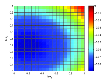
Figure 2: Surface of the MSE difference in a scenario with $S=2$ (SCE). The MSE difference is defined as $\delta{\rm MSE}=\|\mbox{\boldmath{$h$}}-\hat{\mbox{\boldmath{$h$}}}_{\rm b}\|^{2}-\|\mbox{\boldmath{$h$}}-\hat{\mbox{\boldmath{$h$}}}_{\rm RLS}\|^{2}$.

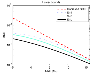
Figure 3: MSE lower bounds for the proposed GSE with different numbers of groups (SCE).

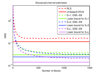
Figure 4: MSE performance with different numbers of groups (SCE). Parameters used: RLS: $\lambda=0.998$, $\delta=10$. Proposed GSE EB: $\mu=0.075$.

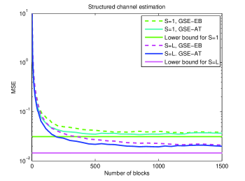
Figure 5: MSE performance of the proposed GSE-EB and GSE-AT algorithms with $S=1$ and $S=L$ (SCE). Parameters used: Proposed GSE-EB: $\mu=0.075$. Proposed GSE-AT: $\mu=0.075$, $\mu_{p}=0.05$.

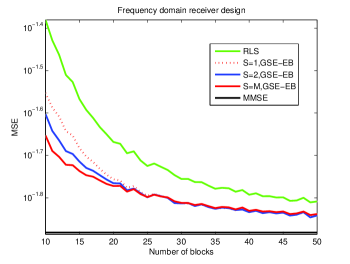
Figure 6: Normalized MSE performance ($\|\mbox{\boldmath{$b$}}-\hat{\mbox{\boldmath{$b$}}}\|^{2}/\|\mbox{\boldmath{$b$}}\|^{2}$) of the biased estimator with 5 users in 5 dB SNR.

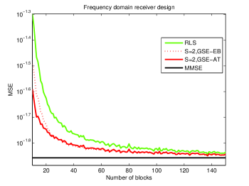
Figure 7: Normalized MSE performance ($\|\mbox{\boldmath{$b$}}-\hat{\mbox{\boldmath{$b$}}}\|^{2}/\|\mbox{\boldmath{$b$}}\|^{2}$) of the biased estimators with 5 users in 3 dB SNR.

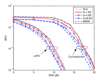
Figure 8: Coded BER performance of the GSE schemes in interference suppression scenario with 5 users.

First, we examine the MSE difference between the unbiased estimator and the proposed GSE as a function of the shrinkage factors for each group in a single user system with 0 dB SNR. In Fig. 2, the surface defined as $\delta{\rm MSE}=\|\mbox{\boldmath{$h$}}-\hat{\mbox{\boldmath{$h$}}}_{\rm b}\|^{2}-\|\mbox{\boldmath{$h$}}-\hat{\mbox{\boldmath{$h$}}}_{\rm RLS}\|^{2}$ in the range of the shrinkage factors between 0 to 1 is shown. Note that, when the bias equals zero, which corresponding to the point $[1,1]$ in the figure, the MSE difference equals zero. The optimal solution is located at $[1+\alpha_{1},1+\alpha_{2}]=[0.15,0.35]$. For this channel realization, the optimal solution that is obtained by our algorithm after transmitting 1000 data blocks is reported as $[1+\alpha_{1},1+\alpha_{2}]=[0.16,0.35]$, which is very close to the optimal solution shown in this figure.

In Fig. 3, the MSE lower bounds for the proposed GSE schemes with different numbers of groups are shown as a function of SNR. The proposed biased estimators show a better performance than the conventional unbiased estimator. As we have proved, the best performance can be obtained in case of $S=L$. The proposed GSE schemes can maintain the MSE gain for low and medium SNR regimes. In high SNR scenarios with a small noise variance, the biased estimator converges to the unbiased estimator and the gain becomes smaller. Compared with the biased estimators with only one shrinkage factor (which is equivalent to the case $S=1$), the GSE schemes with a number of groups can maintain the MSE gain until higher SNR regime.

In the third experiment, we examine the proposed GSE schemes with different numbers of groups for the SCE in a single-user system with 0 dB SNR. In Fig. 4, the MSE performance of the channel estimators are compared as a function of the number of blocks transmitted. The RLS algorithm approaches the unbiased CRLB while the proposed biased estimators approach the lower bounds as given in (61). The biased estimators converge faster than the RLS algorithm and the steady-state performance is also improved. Note that the additional complexity to employ the proposed biased estimation techniques increases linearly with the product of the number of groups and the length of the channel.

In Fig. 5, the proposed GSE-EB and GSE-AT algorithms are compared in $S=1$ and $S=L$ scenarios in a single user system with 0 dB SNR. It can be found that the GSE-AT algorithm can provide a noticeable gain over the GSE-EB algorithm especially at the beginning stage of transmission. This is because the GSE-AT algorithm allows us to further adjust the diagonal matrix $\hat{\mbox{\boldmath{$P$}}}_{m}(i)$ for each time instant. At the beginning stage when the RLS algorithm does not very accurately estimate the channel, the GSE-AT algorithm can be used to improve the convergence rate.

In Fig. 6, the performance of the proposed GSE is shown in the interference suppression scenario (frequency domain receiver design as an example) with a short training sequence. In this simulation, 50 training blocks are transmitted in a scenario with 5 users with 5 dB SNR. The proposed GSE-EB algorithm outperforms the RLS algorithm and the best performance is obtained by setting $S=M$. In Fig. 7, we compare the GSE-EB and GSE-AT algorithms in 5-user communications and an SNR of 3 dB. In this experiment, 150 training blocks are transmitted. The GSE-AT algorithm can further accelerate the convergence rate of the GSE-EB algorithm. At the beginning stage, the GSE-AT algorithm introduces the best performance.

In Fig. 8, the bit error rate (BER) performance of the proposed GSE with different numbers of groups are shown in a scenario with 5 users. The coded BER performance is obtained by adopting a convolutional code and an LDPC code [30] designed according to the PEG approach [30]. For the convolutional code, the constraint length is 5, the rate is 2/3 and the code polynomial is [7,5,5]. For the LDPC code, the rate is 1/2 and the code length is 200 bits. The maximum number of iterations is set to 20. In this experiment, 100 training blocks are transmitted followed by 400 data blocks. With the convolutional code, the proposed GSEs perform better than the RLS algorithm and the maximum gains are obtained in the medium SNR range from 12 dB to 17 dB. By employing the LDPC code, a BER of around $10^{-3}$ is achieved at 12 dB. The proposed GSEs with LDPC codes also outperform the RLS algorithm and the maximum gains are obtained for an SNR around 7 dB.

VII Conclusions

In this work, a novel biased estimation algorithm called group-based shrinkage estimator (GSE) is proposed, which divides the target parameter vector into a number of groups and calculates one shrinkage factor for each group. Adaptive algorithms are developed for the GSE scheme in the parameter estimation and the interference suppression scenarios. The incorporation of the proposed estimators has been considered in the frequency-domain of DS-UWB systems, where structured channel estimation and the receiver designs are considered as examples of the parameter estimation scenario and interference suppression scenario, respectively. An MSE analysis is presented that indicates the lower bound of the proposed GSE schemes. The relationship between the lower bound and the number of groups are also established. It has been proved that the GSE provides a better performance than the biased estimators with only one shrinkage factor. In addition, the lowest MSE lower bound can be obtained in the $S=L$ case. As for future research directions, the GSE scheme can be developed in different systems and scenarios. In addition, if we have some prior knowledge of the target parameter vector, we can then divide it into groups with different sizes and find more attractive tradeoffs between the computational complexity and the performance.

Appendix A MMSE Comparison

In order to check if the objective as shown in (60) is fulfilled with $\mbox{\boldmath{$a$}}_{\rm opt}$, the equation (35) is rearranged by taking the expression of the diagonal matrix $\mbox{\boldmath{$H$}}^{H}\mbox{\boldmath{$H$}}\in\mathbb{C}^{S\times S}$ into account. We have

$$\begin{split}&\boldsymbol{\alpha}_{\rm opt}=[\alpha_{\rm opt,1},\dots,\alpha_{\rm opt,S}]^{T}=-\tilde{\sigma}^{2}\big{(}\tilde{\sigma}^{2}\mbox{\boldmath{$I$}}+\mbox{\boldmath{$H$}}^{H}\mbox{\boldmath{$H$}}\big{)}^{-1}{\bf 1}_{S}\\ &=-[(1+h_{\Sigma,1}/\tilde{\sigma}^{2})^{-1},(1+h_{\Sigma,2}/\tilde{\sigma}^{2})^{-1},\dots,(1+h_{\Sigma,S}/\tilde{\sigma}^{2})^{-1}]^{T}\\ \end{split}$$ (63)

where $h_{\Sigma,s}=\sum^{sL/S}_{i=(s-1)L/S+1}|h(i)|^{2}$. Hence, we have the following expressions

$$\tilde{\sigma}^{2}({\bf 1}_{S}+\boldsymbol{\alpha})^{H}({\bf 1}_{S}+\boldsymbol{\alpha})=\tilde{\sigma}^{2}\sum^{S}_{s=1}(1+\alpha_{\rm opt,s})^{2},$$ (64)

$${\boldsymbol{\alpha}}^{H}\mbox{\boldmath{$H$}}^{H}\mbox{\boldmath{$H$}}{\boldsymbol{\alpha}}=\sum^{S}_{s=1}\alpha_{\rm opt,s}^{2}h_{\Sigma,s}.$$ (65)

By substituting (64) and (65) into the MSE expression (60) and bearing in mind that $S\tilde{\sigma}^{2}=v$, the inequality that we want to prove becomes

$$\tilde{\sigma}^{2}\sum^{S}_{s=1}(1+\alpha_{\rm opt,s})^{2}+\sum^{S}_{s=1}\alpha_{\rm opt,s}^{2}h_{\Sigma,s}-S\tilde{\sigma}^{2}\leq 0.$$ (66)

Note that the left hand-side of (66) can be expressed as

$$\begin{split}&\sum^{S}_{s=1}\alpha_{\rm opt,s}^{2}+\sum^{S}_{s=1}2\alpha_{\rm opt,s}+\sum^{S}_{s=1}\alpha_{\rm opt,s}^{2}h_{\Sigma,s}/\tilde{\sigma}^{2}\\ &=\sum^{S}_{s=1}\alpha_{\rm opt,s}^{2}(1+h_{\Sigma,s}/\tilde{\sigma}^{2})+\sum^{S}_{s=1}2\alpha_{\rm opt,s}.\end{split}$$ (67)

By recalling that $\alpha_{\rm opt,s}=-(1+h_{\Sigma,s}/\tilde{\sigma}^{2})^{-1}$ is always a non-positive scalar value, the left-hand side of the equation becomes

$$\sum^{S}_{s=1}(1+h_{\Sigma,s}/\tilde{\sigma}^{2})^{-1}+\sum^{S}_{s=1}2\alpha_{\rm opt,s}=\sum^{S}_{s=1}\alpha_{\rm opt,s}.$$ (68)

As $\alpha_{\rm opt,s}$ are always non-positive, the summation on the right hand-side of (68) will always be smaller or equal to zero, which completes the proof.

Appendix B Proofs of the statements

First, we want to prove that the lower bound of MSE as shown in (61) with $S>1$ will always be lower than or equal to the $S=1$ case. Based on the equation (61), we can focus on the following function

$$f(S)=\sum^{S}_{s=1}\frac{1}{Sv+h_{\Sigma,s}S^{2}}=\frac{1}{S^{2}}\sum^{S}_{s=1}\frac{1}{(v/S)+h_{\Sigma,s}},$$ (69)

where $h_{\Sigma,s}=\sum^{sL/S}_{i=(s-1)L/S+1}|h(i)|^{2}$ The task now is equivalent to proving that $f(S)\geq f(1)$ for all the possible values of $S$. Note that $\sum^{S}_{s=1}h_{\Sigma,s}=\|\mbox{\boldmath{$h$}}\|^{2}$ and

$$f(1)=\frac{1}{v+\|\mbox{\boldmath{$h$}}\|^{2}}=\frac{1}{v+\sum^{S}_{s=1}h_{\Sigma,s}}=\frac{1}{\sum^{S}_{s=1}(v/S+h_{\Sigma,s})}.$$ (70)

Hence, the relation becomes

$$\sum^{S}_{s=1}\frac{1}{(v/S)+h_{\Sigma,s}}\geq\frac{S^{2}}{\sum^{S}_{s=1}(v/S+h_{\Sigma,s})}.$$ (71)

Actually, we can express this problem as the following mathematical problem:

$$\frac{1}{a_{1}}+\frac{1}{a_{2}}+\dots+\frac{1}{a_{S}}\geq\frac{S^{2}}{\sum^{S}_{s=1}a_{s}},$$ (72)

where $S$ is a positive integer and $a_{s}=(v/S)+h_{\Sigma,s}$ are all non-negative values. This inequality can be proved by using the mathematical induction as follows:
For $S=1$, the left-hand side and the right-hand side are both equal to $\frac{1}{a_{1}}$.
For $S=2$, the left-hand side equals $\frac{1}{a_{1}}+\frac{1}{a_{2}}=\frac{a_{1}+a_{2}}{a_{1}a_{2}}$ and the right-hand side equals $\frac{4}{a_{1}+a_{2}}$. Since $(a_{1}+a_{2})^{2}-4a_{1}a_{2}=(a_{1}-a_{2})^{2}\geq 0$, the inequality holds.
Assuming the inequality holds for $S=n$, where $n\geq 2$, we have

$$\frac{1}{a_{1}}+\frac{1}{a_{2}}+\dots+\frac{1}{a_{n}}\geq\frac{n^{2}}{\sum^{n}_{s=1}a_{s}}.$$ (73)

For $S=n+1$, we first consider the left-hand side as follows

$$\begin{split}\frac{1}{a_{1}}+\frac{1}{a_{2}}+\dots+\frac{1}{a_{n}}+\frac{1}{a_{n+1}}&\geq\frac{n^{2}}{\sum^{n}_{s=1}a_{s}}+\frac{1}{a_{n+1}}\\ &=\frac{n^{2}a_{n+1}+\sum^{n}_{s=1}a_{s}}{(\sum^{n}_{s=1}a_{s})\cdot a_{n+1}}.\end{split}$$ (74)

and then, the right-hand side is given by

$$\frac{(n+1)^{2}}{\sum^{n}_{s=1}a_{s}+a_{n+1}}.$$ (75)

Because

$$\begin{split}&\big{(}\sum^{n}_{s=1}a_{s}+a_{n+1}\big{)}\big{(}n^{2}a_{n+1}+\sum^{n}_{s=1}a_{s}\big{)}-(n+1)^{2}\big{(}\sum^{n}_{s=1}a_{s}\big{)}\cdot a_{n+1}\\ &=\big{(}\sum^{n}_{s=1}a_{s}-n\cdot a_{n+1}\big{)}^{2}\geq 0,\end{split}$$

the inequality also holds for $S=n+1$. This completes the proof.

Now, we can prove the second statement which points out that the lowest MSE lower bound as shown in (61) can be obtained when the numbers of groups is equal to the length of the parameter vector to be estimated. Following the proof of of $Statement$ 1, we can express the problem that needs to be solved as: prove that $f(L)\geq f(S)$, for any possible values of number of groups $S$, and mathematically, we need to prove that

$$\frac{1}{L^{2}}\sum^{L}_{i=1}\frac{1}{(v/L)+|h(i)|^{2}}\geq\frac{1}{S^{2}}\sum^{S}_{s=1}\frac{1}{(v/S)+h_{\Sigma,s}},$$ (76)

holds for all the possible values of $S$. Since the parameter vector is divided into a number of $S$ groups, this inequality holds if the following relationship is fulfilled:

$$\begin{split}&\frac{1}{L^{2}}\sum^{sL/S}_{i=(s-1)L/S+1}\frac{1}{(v/L)+|h(i)|^{2}}\geq\frac{1}{S^{2}}\frac{1}{(v/S)+h_{\Sigma,s}},\\ &\hskip 10.00002ptwith\hskip 5.0pts=1,2,\dots,S\end{split}$$ (77)

Actually, the $S=L$ case can be considered as the division of each group (with length $L/S$) into a number of $L/S$ length-one sub-groups, and the inequality of (77) always holds for each group because of $Statement$ 1. This completes the proof.

Sheng Li (S’08 - M’11) received his Bachelor Degree in Zhejiang University of Technology in China in 2006 and the M.Sc. degree in communications engineering and Ph.D. degree in electronics engineering, both from the University of York, U.K. in 2007 and 2010, respectively. In 2010, he was awarded the K. M. Stott prize for excellence in scientific research. During November 2010 to October 2011, he has carried out a postdoctoral research in the Ilmenau University of Technology, Germany. Since April 2012, he has been with Zhejiang University of Technology, China, where he is currently a lecturer.

Rodrigo C. de Lamare (S’99 - M’04 - SM’10) received the Diploma in electronic engineering from the Federal University of Rio de Janeiro (UFRJ) in 1998 and the M.Sc. and PhD degrees, both in electrical engineering, from the Pontifical Catholic University of Rio de Janeiro (PUC-Rio) in 2001 and 2004, respectively. Since January 2006, he has been with the Communications Research Group, Department of Electronics, University of York, where he is currently a Reader. Since April 2011, he has also been a Professor with PUC-RIO. His research interests lie in communications and signal processing, areas in which he has published nearly 300 papers in refereed journals and conferences. Dr. de Lamare serves as associate editor for the EURASIP Journal on Wireless Communications and Networking. He is a Senior Member of the IEEE has served as the General Chair of the 7th IEEE International Symposium on Wireless Communications Systems (ISWCS), held in York, UK in September 2010, and will serve as the Technical Programme Chair of ISWCS 2013 in Ilmenau, Germany.

Martin Haardt (S’90 - M’98 - SM’99) has been a Full Professor in the Department of Electrical Engineering and Information Technology and Head of the Communications Research Laboratory at Ilmenau University of Technology, Germany, since 2001. Since 2012, he has also served as an Honorary Visiting Professor in the Department of Electronics at the University of York, UK. After studying electrical engineering at the Ruhr-University Bochum, Germany, and at Purdue University, USA, he received his Diplom-Ingenieur (M.S.) degree from the Ruhr-University Bochum in 1991 and his Doktor-Ingenieur (Ph.D.) degree from Munich University of Technology in 1996. In 1997 he joint Siemens Mobile Networks in Munich, Germany, where he was responsible for strategic research for third generation mobile radio systems. From 1998 to 2001 he was the Director for International Projects and University Cooperations in the mobile infrastructure business of Siemens in Munich, where his work focused on mobile communications beyond the third generation. During his time at Siemens, he also taught in the international Master of Science in Communications Engineering program at Munich University of Technology. Martin Haardt has received the 2009 Best Paper Award from the IEEE Signal Processing Society, the Vodafone (formerly Mannesmann Mobilfunk) Innovations-Award for outstanding research in mobile communications, the ITG best paper award from the Association of Electrical Engineering, Electronics, and Information Technology (VDE), and the Rohde and Schwarz Outstanding Dissertation Award. In the fall of 2006 and the fall of 2007 he was a visiting professor at the University of Nice in Sophia-Antipolis, France, and at the University of York, UK, respectively. His research interests include wireless communications, array signal processing, high-resolution parameter estimation, as well as numerical linear and multi-linear algebra. Prof. Haardt has served as an Associate Editor for the IEEE Transactions on Signal Processing (2002-2006 and since 2011), the IEEE Signal Processing Letters (2006-2010), the Research Letters in Signal Processing (2007-2009), the Hindawi Journal of Electrical and Computer Engineering (since 2009), the EURASIP Signal Processing Journal (since 2011), and as a guest editor for the EURASIP Journal on Wireless Communications and Networking. He has also served as an elected member of the Sensor Array and Multichannel (SAM) technical committee of the IEEE Signal Processing Society (since 2011), as the technical co-chair of the IEEE International Symposiums on Personal Indoor and Mobile Radio Communications (PIMRC) 2005 in Berlin, Germany, as the technical program chair of the IEEE International Symposium on Wireless Communication Systems (ISWCS) 2010 in York, UK, as the general chair of ISWCS 2013 in Ilmenau, Germany, and as the general-co chair of the 5-th IEEE International Workshop on Computational Advances in Multi-Sensor Adaptive Processing (CAMSAP) 2013 in Saint Martin, French Caribbean.

References

- [1] R. C. de Lamare, M. Haardt, and R. Sampaio-Neto, “Blind Adaptive Constrained Reduced-Rank Parameter Estimation based on Constant Modulus Design for CDMA Interference Suppression,” IEEE Trans. Signal Process., vol. 56, no. 6, pp. 2470-2482, June 2008.
- [2] R. C. de Lamare and R. Sampaio-Neto, “Reduced-Rank Space-Time Adaptive Interference Suppression With Joint Iterative Least Squares Algorithms for Spread-Spectrum Systems,” IEEE Trans. Veh. Technol., vol.59, no.3, pp.1217-1228, Mar. 2010.
- [3] Z. Wang, Y. Xin, G. Mathew, and X. Wang, “A Low-Complexity and Efficient Channel Estimator for Multiband OFDM-UWB Systems,” IEEE Trans. Veh. Technol., vol.59, no.3, pp.1355-1366, Mar. 2010.
- [4] Q. Z. Ahmed, L. L. Yang, and Sheng Chen, “Reduced-Rank Adaptive Least Bit-Error-Rate Detection in Hybrid Direct-Sequence Time-Hopping Ultrawide Bandwidth System,” IEEE Trans. Veh. Technol., vol.60, no.3, pp.849-857, Mar. 2011.
- [5] M. Marques da Silva et al.,Transmission Techniques for Emergent Multicast and Broadcast Systems, CRC Press Auerbach Publications, 1st Edition, ISBN: 9781439815939, Boca Raton, USA, May 2010.
- [6] S. M. Kay, Fundamentals of Statistical Signal Processing: Estimation Theory, Upper Saddle River, NJ:Prentice Hall, 1993.
- [7] Y. C. Eldar, A. Ben-Tal, and A. Nemirovski, “Robust Mean-Squared Error Estimation in the Presence of Model Uncertainties,” IEEE Journal on Signal Processing, vol. 53, no. 1, pp. 168-181, Jan. 2005.
- [8] Y. C. Eldar, “Rethinking Biased Estimation: Improving Maximum Likelihood and the Cramèr-Rao Bound,” Foundations and Trends in Signal Processing, vol. 1, no. 4, pp. 305-449, 2008.
- [9] S. Kay and Y. C. Eldar, “Rethinking Biased Estimation,” IEEE Signal Process. Mag., pp. 133-136, May. 2008.
- [10] W. James and C. Stein, “Estimation with quadratic loss,” Proc. 4th Berkeley Symp. Mathematical Statistics and Probability, Berkeley, CA, vol. 1, pp.361-379, 1961.
- [11] J. R. Thompson, “Some Shrinkage Techniques for Estimating the Mean,” Journal of the American Statistical Association, vol. 63, no. 321, pp. 113-122, Mar. 1968.
- [12] M. E. Bock, “Minimax estimators of the mean of a multivariate normal distribution,” The Annals of Statistics, vol. 3, no. 1, pp. 209-218, Jan. 1975.
- [13] S. Li, R. C. de Lamare, and M. Haardt, “Linear interference suppression in the frequency domain for DS-UWB systems using biased RLS estimation with adaptive shrinkage factors,” in European Wireless (EW), Apr. 2011.
- [14] S. Li, R. C. de Lamare, and M. Haardt, “Adaptive frequency-domain biased estimation algorithms with automatic adjustment of shrinkage factors,” in Proc. IEEE Int. Conference on Acoustics, Speech, and Signal Processing (ICASSP), pp. 4268 - 4271, May 2011.
- [15] J. H. Manton, V. Krishnamurthy, and H. V. Poor, “James-Stein State Filtering Algorithms,” IEEE Trans. Signal Process., vol. 46, no. 9, pp. 2431-2447, Sep. 1998.
- [16] Z. Ben-Haim and Y. C. Eldar, “Blind Minimax Estimation,” IEEE Trans. Inf. Theory, vol. 53, no. 9, pp. 3145-3157, Sep. 2007.
- [17] G. Durisi and S. Benedetto, “Performance evaluation of TH-PPM UWB systems in the presence of multiuser interference,” IEEE Commun. Lett., vol. 7, pp. 224-226, May 2003.
- [18] R. Fisher, R. Kohno, and M. M. Laughlin et al., “DS-UWB Physical Layer Submission to IEEE 802.15 Task Group 3a (Doc. Number P802.15-04/0137r4),” IEEE P802.15, Jan. 2005.
- [19] A. F. Molisch, D. Cassioli, and C. C. Chong et al., “A Comprehensive Standardized Model for Ultrawideband Propagation Channels,” IEEE Trans. Antennas Propag., vol. 54, no. 11, pp. 3151-3166, Nov. 2006.
- [20] M. Morelli, L. Sanguinetti and U. Mengali, “Channel Estimation for Adaptive Frequency-Domain Equalization,” IEEE Trans. Wireless Commun., vol. 4, no. 5, pp. 2508-2518, Sep. 2005.
- [21] S. Li and R. C. de Lamare, “Frequency Domain Adaptive Detectors for SC-FDE in Multiuser DS-UWB Systems Based on Structured Channel Estimation and Direct Adaptation,” IET Communications, vol. 4, issue. 13, pp. 1636-1650, 2010.
- [22] M. Biguesh and A. B. Gershman, “Training-Based MIMO Channel Estimation: A Study of Estimator Tradeoffs and Optimal Training Signals,” IEEE Trans. Signal Process., vol. 54, no. 3, pp. 884-893, Mar. 2006.
- [23] J. J. de Beek, O. Edfors, M. Sandell, S. K. Wilson, and P. O. Borjesson, “On Channel Estimation in OFDM Systems,” in Proc. IEEE VTC, pp. 815 - 819, Jul. 1995.
- [24] O. Edfors, M. Sandell, J. J. de Beek, S. K. Wilson, and P. O. Borjesson, “OFDM Channel Estimation by Singular Value Decomposition,” IEEE Trans. Commun., vol. 46, no. 7, pp. 931-939, Sep. 1998.
- [25] A. F. Molisch, D. Cassioli, and C. C. Chong et al., “A Comprehensive Standardized Model for Ultrawideband Propagation Channels,” IEEE Trans. Antennas Propagat., vol. 54, no. 11, pp. 3151-3166, Nov. 2006.
- [26] M. X. Chang and C.C. Yang, “A Novel Architecture of Single-Carrier Block Transmission DS-CDMA,” in IEEE Vehicular Technology Conference (VTC), Sep. 2006.
- [27] S. Haykin, Adaptive Filter Theory, 4th Edition, Pearson Education, 2002.
- [28] J. Teng, H Snoussi, C. Richard, and R. Zhou, “Distributed Variational Filtering for Simultaneous Sensor Localization and Target Traching in Wireless Sensor Networks,” IEEE Trans. Veh. Technol., vol.61, no.5, pp.2305-2318, Jun. 2012.
- [29] D. B. Jourdan, D. Dardari, and M. Z. Win, “Position Error Bound for UWB localization in Dense Cluttered Environments,” IEEE Trans. Aero. Elec. Sys., vol. 444, no. 2, pp. 613-628, Apr. 2008.
- [30] W. Ryan and S. Lin, Channel Codes: Classical and Modern, Cambridge University Press, 2009.
- [31] K. Todros and J. Tabrikian, “Uniformly Best Biased Estimators in Non-Bayesian Parameter Estimation,” IEEE Trans. Inf. Theory, vol. 57, no. 11, pp. 7635-7647, 2011.
- [32] M. L. Honig and J. S. Goldstein,“Adaptive reduced-rank interference suppression based on the multistage Wiener filter,” IEEE Trans. Commun., vol. 50, no. 6, pp. 986-994, Jun. 2002.
- [33] D. A. Pados, G. N. Karystinos, “An iterative algorithm for the computation of the MVDR filter,” IEEE Trans. Sig. Proc., vol. 49, No. 2, February, 2001.
- [34] S. Li and R. C. de Lamare, “Reduced-Rank Linear Interference Suppression for DS-UWB Systems Based on Switched Approximations of Adaptive Basis Functions,” IEEE Trans. Veh. Technol., vol. 60, no. 2, pp. 485-497, Feb. 2011.
- [35] R. C. de Lamare and R. Sampaio-Neto, “Adaptive Reduced-Rank Processing Based on Joint and Iterative Interpolation, Decimation, and Filtering,” IEEE Trans. Sig. Proc., vol. 57, no. 7, pp. 2503 - 2514, July 2009.