Differential Geometrically Consistent
Artificial Viscosity in Curvilinear Coordinates

Abstract

High-resolution numerical methods have been developed for nonlinear, discontinuous problems as they appear in simulations of astrophysical objects. One of the strategies applied is the concept of artificial viscosity. Grid-based numerical simulations ideally utilize problem-oriented grids in order to minimize the necessary number of cells at a given (desired) spatial resolution. We want to propose a modified tensor of artificial viscosity which is employable for generally comoving, curvilinear grids.We study a differential geometrically consistent artificial viscosity analytically and visualize a comparison of our result to previous implementations by applying it to a simple self-similar velocity field. We give a general introduction to artificial viscosity first and motivate its application in numerical analysis. Then we present how a tensor of artificial viscosity has to be designed when going beyond common static Eulerian or Lagrangian comoving rectangular grids. We find that in comoving, curvilinear coordinates the isotropic (pressure) part of the tensor of artificial viscosity has to be modified metrically in order for it to fulfill all its desired properties.

1 Introduction

In astrophysics a multitude of systems and configurations are described with concepts from hydrodynamics, often combined with gravitation, radiation and/or magnetism. Mathematically radiation hydrodynamics (RHD) and magnetohydrodynamics (MHD) are described by systems of coupled nonlinear partial differential equations. The Euler equations of hydrodynamics, the Maxwell equations as well as radiative transport equations are hyperbolic PDEs that connect certain densities and fluxes via conservation laws. The numerical solutions of these equations essentially need to comprise this quality. Today there exists a wide range of numerical methods for conservation laws that ensure the conservation of mass, momentum, energy etc. if applied properly, and multiple fields in physics and astrophysics have adopted these sophisticated numerical methods for studying various applications.

Standard numerical schemes for partial differential equations are established under the assumption of classical differentiability. Routine finite difference schemes of first order usually smear or smoothen the solution in the vicinity of discontinuities as they come with intrinsic numerical viscosity. Standard second order methods show something to the effect of the Gibbs phenomenon, where oscillations around shocks emerge. In the past decades so called high-resolution methods have been developed in order to achieve proper accuracy and resolution for nonlinear, discontinuous problems as they appear also in RHD or MHD. One of these strategies is the concept of artificial viscosity which we will also briefly motivate in subsection 1.1.

In higher-dimensional problems this artificial viscosity emerges as a tensorial quantity. We will demonstrate this in subsection 1.3. The result we want to present in this paper can be seen as a tensor analytical consequence of the artificial viscosity in general curvilinear coordinates when using consistent metric tensors. In section 2 we will propose a correction for the commonly used tensor of artificial viscosity for curvilinear grids.

This correction is motivated by astrophysical applications where one considers comoving nonlinear coordinates represented by non-conformal (non-angle preserving) maps from spherical coordinates. The authors are currently investigating the generation of grids that are asymptotically spherical but which allow certain asymmetries that can be found in rotating configurations, nonlinear pulsation processes etc. This new approach to grid-based astrophysical simulation techniques will be addressed extensively with numerical applications in a future paper.

As an example of non-conformal two dimensional coordinates, Figure 1 shows a grid that corresponds to the map $(x,y)\to(\xi,\eta)$,

$$x=\xi\cos\eta$$ (1)

$$y=(a_{1}\xi+a_{2}\xi^{2})\Big{(}1+\frac{a_{3}\pi^{3}-16a_{2}\xi+a_{2}a_{3}\pi^{3}\xi}{4\pi(1+a_{2}\xi)}\eta\,\,+$$

$$+\,\frac{4a_{2}\xi-a_{3}\pi^{3}-a_{2}a_{3}\pi^{3}\xi}{\pi^{2}(1+b_{2}\xi)}\eta^{2}+a_{3}\eta^{3}\Big{)}\sin\eta$$

which gives the polar coordinates for the choice of parameters $(a_{1},a_{2},a_{3})=(1,0,0).$ In such a nonorthogonal grid the metric tensor is no longer diagonal and one has to consider a consistent differential geometric approach to the formulation of the governing equations of RHD and MHD, and also to the mathematical formulation of the artificial viscosity, which will be stressed in Section 2.

The benefit of the consistent formulation can be seen when we consider time-dependent grids, e.g. when using time-dependent parameters $(a_{1},a_{2},a_{3})$ in (1).

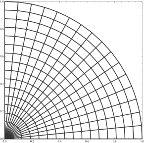
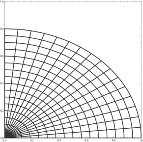
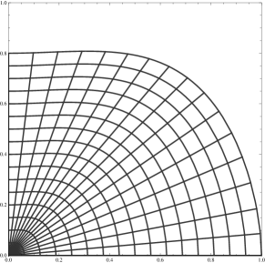
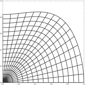
Figure 1: Example of a non-conformal non-steady 2D grid with oblateness governed by three choices of parameters $(a_{1},a_{2},a_{3})$ as defined in equation (1).

We refer to the Appendix 5 for the depiction of the system of equations of RHD for generally comoving curvilinear coordinates with time-dependent metrics correspondingly.

1.1 Brief Introduction to Conservation Laws

For the sake of stringency we recapitulate some important results from the theory and numerics of conservation laws which can be found e.g. in (LeVeque, 1991) or  (Richtmyer and Morton, 1994).

The equations of RHD and MHD form a system of hyperbolic conservation laws that describe the interaction of a density function $\mathbf{d}\left(\mathbf{x},t\right):\mathbb{R}^{n}\times\left[0,\infty\right)\rightarrow\mathbb{R}^{m}$ and its flux $\mathbf{f}\left(\mathbf{d}\right):\mathbb{R}^{m}\rightarrow\mathbb{R}^{m\times n}$. Equation (6) shows how a concrete choice for the density and the flux field can look like in a given coordinate system.

The temporal change of the integrated density in a connected set $\Omega\subset\mathbb{R}^{n}$ then equals the flux over the boundary $\partial\Omega$, i.e.

$$\quad\partial_{t}\int\limits_{\Omega}\mathbf{d}\,\,\d{V}+\int\limits_{\partial\Omega}\mathbf{f}\cdot\mathbf{n}\,\d{S}=\mathbf{0}\quad\textrm{for all }\,\,t>0,$$ (2)

where $\mathbf{n}$ is the outward oriented normal of the surface.

The system is called hyperbolic if the Jacobian matrix $\nabla_{\mathbf{d}}\mathbf{f}$ associated with the fluxes has real eigenvalues and if there exists a complete set of eigenvectors. In case of MHD and RHD this property has a direct physical relevance (Pons et al., 2000).

Assuming $\mathbf{f}$ to be a continuously differentiable function, equation (2) can be rewritten via the divergence theorem as

$$\int\limits_{t}\int\limits_{\Omega}\big{(}\partial_{t}\mathbf{d}+\mathrm{div}_{\mathbf{x}}\,\mathbf{f}(\mathbf{d})\big{)}\,\d{V}\,\d{t}=\mathbf{0}\quad\textrm{ for all }\,\,t>0,\,\Omega\subset\mathbb{R}^{n},$$ (3)

which gives the system of partial differential equations for the density function $\mathbf{d}$:

$$\partial_{t}\mathbf{d}+\mathrm{div}_{\mathbf{x}}\,\mathbf{f}(\mathbf{d})=\mathbf{0}\quad\textrm{ for all }\,\,t>0,\,\mathbf{x}\in\mathbb{R}^{n}.$$ (4)

With an initial condition $\mathbf{d}(\mathbf{x},0)=\mathbf{d}_{0}(\mathbf{x})$, $\mathbf{x}\in\mathbb{R}^{n}$, this is called the Cauchy problem.

In order to illustrate the connection of hydrodynamical applications to this formalism, we express the Euler equations in the form (4). The appearing variables are the gaseous density $\rho(\mathbf{x},t)$, the gas velocity $\mathbf{u}(\mathbf{x},t)$, the inner energy $\epsilon(\mathbf{x},t)$ and the gaseous pressure tensor $\mathbf{P}(\mathbf{x},t)$. Considering the differential form (4), we recognize the continuity equation, the equation of motion and the energy equation as the components of the hyperbolic problem. In case of the most relevant problem, that of 3D hydrodynamics, the density and its flux are given as

$$\mathbf{d}=\begin{pmatrix}\rho\vspace{1mm}\\ \rho\mathbf{u}\vspace{1mm}\\ \rho\epsilon\end{pmatrix}\in\mathbb{R}^{5},\quad\mathbf{f}(\mathbf{d})=\begin{pmatrix}\rho\mathbf{u}^{\mathrm{T}}\vspace{1mm}\\ \rho\mathbf{u}\mathbf{u}^{\mathrm{T}}+\mathbf{P}\vspace{1mm}\\ \rho\epsilon\mathbf{u}+(\mathbf{P}\mathbf{u})^{\mathrm{T}}\end{pmatrix}\in\mathbb{R}^{5\times 3}.$$ (5)

For a given coordinate system with base vectors $\mathbf{e}_{i}$, the tensorial fields are given explicitly as (using the Einstein notation)

$$\mathbf{d}=\begin{pmatrix}\rho\vspace{1mm}\\ \rho u^{i}\,\mathbf{e}_{i}\vspace{1mm}\\ \rho\epsilon\end{pmatrix},\quad\mathbf{f}(\mathbf{d})=\begin{pmatrix}\rho u^{i}\,\mathbf{e}_{i}^{\mathrm{T}}\vspace{1mm}\\ \big{(}\rho u^{i}u^{j}+P^{ij}\big{)}\,\mathbf{e}_{i}\mathbf{e}_{j}^{\mathrm{T}}\vspace{1mm}\\ \big{(}\rho\epsilon u^{i}+{P^{i}}_{j}u^{j}\big{)}\,\mathbf{e}_{i}^{\mathrm{T}}\end{pmatrix}.$$ (6)

The gaseous pressure tensor can be assumed to be isotropic in most applications, which means that $\mathbf{P}=g^{ij}p$ where $p(\mathbf{x},t)$ is the scalar gas pressure and $g^{ij}={\mathbf{e}^{i}}^{\mathrm{T}}\mathbf{e}^{j}$ the contravariant metric tensor. In case of adaptive grids respectively moving coordinate lines, the base vectors are time-dependent as well, i.e. then $\mathbf{e}_{i}=\mathbf{e}_{i}(\mathbf{x},t)$.

Since even the simplest examples of one-dimensional scalar conservation laws like the Burgers’ equation have classical solutions only in some special cases, one has to broaden the considered function space of possible solutions. For the so-called weak solutions, we appeal to generalized functions where the discontinuities are defined properly. The generalized concept of differentiation of distributions shifts the operations to test functions $\gamma:\mathbb{R}^{n}\times\mathbb{R}^{+}\supset G\rightarrow\mathbb{R}$ ($G$ open) which are infinitely differentiable and have a compact support (meaning that for each $\gamma$ there exists a closed and bounded subset $K$ such that $\gamma(\mathbf{x},t)=0$ for all $x\,\in G\setminus K$). We denote this space of test functions by $D(G)$. In this generalized space of solutions the Cauchy problem (3) is written as

$$\int_{t\geq 0}\int_{\mathbb{R}^{n}}\big{(}\partial_{t}\mathbf{d}+\mathrm{div}_{\mathbf{x}}\,\mathbf{f}(\mathbf{u})\big{)}\gamma\,\d{V}\,\d{t}=0\,\quad\textrm{for all }\,\gamma\in D(G).$$

The weak formulation of the conservation law (3) is obtained by shifting the derivatives to the test functions by partial integration, and by using the compactness of the support. We get that the following has to hold for each $\gamma\in D(G)$:

$$\int\limits_{t\geq 0}\int\limits_{\mathbb{R}^{n}}\big{(}\mathbf{d}\,\partial_{t}\gamma+\mathbf{f}(\mathbf{d})\,\nabla_{\mathbf{x}}\,\gamma\big{)}\,\d{V}\,\d{t}=-\int\limits_{\mathbb{R}^{n}}\gamma(\mathbf{x},0)\,\mathbf{d}_{0}(\mathbf{x})\,\d{V}.$$ (7)

The function $\mathbf{d}\in L^{\infty}$ is called a weak solution of the PDE (4), if it satisfies (7) and $\mathbf{d}\in U$ with $\mathbf{d}_{0}\in L^{\infty}$. However, there is a small drawback. This weak solution is not necessarily unique and usually further constraints have to be imposed in order to guarantee its uniqueness. This leads us to the actual topic of this paper.

1.2 Introduction to Artificial Viscosity

For most physical problems it is naturally sufficient to look for weak solutions from the function space of piecewise continuously differentiable functions. Constraining the space of solutions in this way, we call the physical variables $\mathbf{d}$ weak solutions of the Cauchy problem (4), if they are classical solutions wherever they are continuously differentiable, and if at discontinuities (shocks) they satisfy additional conditions in order to be physically reasonable (we elaborate on these conditions below).

The mathematical theory provides several techniques to distinguish physically valuable solutions out of a manifold of mathematically possible. One method is to add an artificial viscosity term to the right hand side of (4), to get the equation:

$$\partial_{t}\mathbf{d}+\mathrm{div}_{\mathbf{x}}\,\mathbf{f}(\mathbf{d})=\varepsilon\nu\Delta\mathbf{d},\qquad\varepsilon>0$$ (8)

and then consider the limiting case $\varepsilon\rightarrow 0$. This idea is motivated by physical diffusion which broadens sincere discontinuities to differentiable steep gradients at the (microscopic) length scale of the mean free path of the particles. The physical solution of the weakly formulated problem is thus the zero diffusion limit of the diffusive problem. However, in practice this limit is difficult to calculate analytically, and hence simpler conditions have to be found. A common technique to do this is motivated by continuum physics as well. Here an additional conservation law is set to hold for another quantity - the entropy of the fluid flow - as long as the solution remains smooth. Moreover, it is known that along admissible shocks this physical variable never decreases, and the conservation law for the entropy can be formulated as an inequality.

We denote the (scalar valued) entropy function by $\sigma(\mathbf{d})$ and the entropy flux function by $\phi(\mathbf{d})$, and they satisfy

$$\partial_{t}\sigma(\mathbf{d})+\mathrm{div}_{\mathbf{x}}\,\phi(\mathbf{d})=0.$$ (9)

Assuming the functions to be differentiable, we may rewrite this conservation law via the chain rule and the equation (4) as

$$\nabla_{\mathbf{d}}\sigma(\mathbf{d})\,\mathrm{div}_{\mathbf{x}}\,\mathbf{f}(\mathbf{d})=\mathrm{div}_{\mathbf{x}}\,\phi(\mathbf{d}),$$ (10)

where in higher-dimensional case the appearing matrices of gradients have to fulfillfurther constraints, see e.g. (Godlewski and Raviart, 1992). For scalar equations, it is always possible to find an entropy function of this kind. Furthermore it is assumed that the entropy function is convex, i.e.

$$\nabla_{\mathbf{d}}^{2}\sigma>0,\qquad\textrm{ for all }\,\mathbf{d}\in U.$$ (11)

To get our actual entropy condition, we first rewrite our entropical conservation law (9) in the viscous form

$$\partial_{t}\sigma(\mathbf{d})+\mathrm{div}_{\mathbf{x}}\,\phi(\mathbf{d})=\varepsilon\nabla_{\mathbf{d}}\sigma(\mathbf{d})\Delta\mathbf{d}.$$ (12)

Integrating over an arbitrary time interval $\left[t_{0},t_{1}\right]$ and a connected set $\Omega\subset\mathbb{R}^{n}$, and using partial integration, we find that

$$\int\limits_{t_{0}}^{t_{1}}\int\limits_{\Omega}\left(\partial_{t}\sigma(\mathbf{d})+\mathrm{div}_{\mathbf{x}}\,\phi(\mathbf{d})\right)\,\d{V}\,\d{t}$$ (13)

$$= \varepsilon\int\limits_{t_{0}}^{t_{1}}\int\limits_{\partial\Omega}\left(\nabla_{\mathbf{x}}\mathbf{d}\,\nabla_{\mathbf{d}}\sigma(\mathbf{d})\right)\cdot\mathbf{n}\,\d{S}\,\d{t}$$

$$- \varepsilon\int\limits_{t_{0}}^{t_{1}}\int\limits_{\Omega}\nabla_{\mathbf{x},i}{\mathbf{d}}\,\underbrace{\nabla^{2}\sigma(\mathbf{d})}_{>0}\,\nabla_{\mathbf{x},i}\mathbf{d}\,\d{V}\,\d{t}.$$

When we now consider our non-diffusive limit $\varepsilon\to 0$, the first term on the right-hand side vanishes without further restriction whereas the second term has to remain nonpositive. With partial integration and divergence theorem we get our entropy condition

$$\int\limits_{\Omega}\sigma(\mathbf{d}(\mathbf{x},t_{1}))\,\d{V} \leq\int\limits_{\Omega}\sigma(\mathbf{d}(\mathbf{x},t_{0}))\,dV$$ (14)

$$-\int\limits_{t_{0}}^{t_{1}}\int\limits_{\partial\Omega}\phi(\mathbf{d})\cdot\mathbf{n}\,\d{S}\,\d{t}.$$

For bounded, continuous pointwise solutions $\mathbf{d}^{*}$ of (12) such that $\mathbf{d}^{*}\to\mathbf{d}$ for $\varepsilon\to 0$, the vanishing viscosity solution $\mathbf{d}$ is a weak solution of the initial value problem (3) and fulfills entropy condition (14). Generally spoken, applying the entropy condition to systems with shock solutions unveils those propagation velocities that ensure that no characteristics rise from discontinuities which would be non-physical. For detailed motivation, stringent argumentation and proofs to mathematical techniques presented in this section we refer to (Harten et al., 1976) respectively to (LeVeque, 1991).

1.3 Numerical Artificial Viscosity

As mentioned we are looking for high-resolution methods for nonlinear PDEs derived from hyperbolic conservation laws. In the past decades major efforts have been made in developing numerical methods for these problems that are at least of second order. One patent attempt to finding such a high-resolution method is to adapt a well-known high-order method for linear problems for nonlinear problems (such as the Lax-Wendroff scheme (Lax and Wendroff, 1960)).

As illustrated above we can add an artificial viscosity term to the conservation law in a way that the entropy condition is satisfied and non-physical solutions are excluded. We are keen to design this viscosity in such a manner that it affects sincere discontinuities but vanishes sufficiently elsewhere so that the order of accuracy can be maintained in those regimes where the solution is smooth. The idea of numerical artificial viscosity was inspired by physical dissipation mechanisms and dates back more than half a century to (von Neumann and Richtmyer, 1950).

We denote as customary the approximate solution of the exact density $\mathbf{d}(x,t)$ at discrete grid points $\mathbf{d}(x_{j},t_{n})$ by $\mathbf{D}^{n}_{j}$, and set $\mathbf{D}=\left[\mathbf{D}_{1}\ldots\mathbf{D}_{k}\right]^{\mathrm{T}}$, where $k$ is the total number of grid points. The numerical representation of the flux function $\mathbf{f}(\mathbf{d})$ is denoted respectively by $\mathbf{F}(\mathbf{D})$, where $\left[\mathbf{F}(\mathbf{D})\right]_{j}=\mathbf{f}(\mathbf{D}_{j})$. The numerical flux function gets modified by a an artificial viscosity $\mathbf{Q}\left[\mathbf{D}\right]_{j}$ for instance in the following way:

$$\left[\mathbf{F}_{\text{visc}}(\mathbf{D})\right]_{j}=\left[\mathbf{F}(\mathbf{D})\right]_{j}-h\left[\mathbf{Q}\big{(}\mathbf{D}\big{)}\right]_{j}\big{(}\mathbf{D}_{j+1}-\mathbf{D}_{j}\big{)}.$$ (15)

where $h$ denotes the size of the spatial discretization. Since the original design of this additional viscous pressure in the scalar form $Q=c_{2}\rho(\Delta\mathbf{u})^{2}$, $c_{2}\in\mathbb{R}$ as suggested in (von Neumann and Richtmyer, 1950) for one dimensional advection $\partial_{t}\mathbf{d}+a\partial_{x}\mathbf{d}=Q\partial_{xx}\mathbf{d}$, it has undergone a number of modifications and generalizations. It has turned out to be numerically preferable to add a linear term (see (Landshoff, 1955)) in order to control oscillations. Generalizations to multi-dimensional flows mostly retain the original analogy to physical dissipation and reformulate the velocity term accordingly, see e.g. (Wilkins, 1980).

The artificial viscosity broadens shocks to steep gradients at some characteristic length scale, but should not cause too large smearing. The concrete composition and implementation of this artificial viscosity coefficient $\mathbf{Q}$ depends on the application. As an example we discuss the following form of the tensor of the artificial viscosity in higher-dimensional RHD numerics. Similar forms of artificial viscosity can be found also in pure hydrodynamics and MHD calculations in 2D and 3D.

Tscharnuter and Winkler (Tscharnuter and Winkler, 1979) have pointed out that the viscous pressure in 3D radiation hydrodynamics has to unravel normal stress, quantified by the divergence of the velocity field and shear stress, which is expressed by the symmetrized gradient of the velocity field according to the general theory of viscosity. It is designed to switch on only in case of compression ($\mathrm{div}_{\mathbf{x}}\,\mathbf{u}<0$), and this is all ensured by the form

$$\mathbf{Q}=-q_{2}^{2}l_{\text{visc}}^{2}\rho\max(-\mathrm{div}_{\mathbf{x}}\,\mathbf{u},0)\left(\Big{[}\nabla\mathbf{u}\Big{]}_{s}-\frac{1}{3}\mathbf{e}\,\mathrm{div}_{\mathbf{x}}\,\mathbf{u}\right),$$ (16)

where the symmetrization rule is defined componentwise for the lower indices as

$${\left([\nabla\mathbf{u}]_{s}\right)}_{ij}=\frac{1}{2}(\nabla_{i}u_{j}+\nabla_{j}u_{i}).$$

2 Numerical Artificial Viscosity in Curvilinear Coordinates

We introduced artificial viscosity in form of a three dimensional viscous pressure tensor (16) in section 1.3 along the lines of (Tscharnuter and Winkler, 1979). In this section we want to point out, how such a definition must be adapted for curvilinear coordinates in order to ensure tensor analytical consistency.

When formulating PDEs derived from hyperbolic conservation laws on a curvilinear grid, the tensorial equations (3) have to be transformed to the according coordinate system. Not only the vectorial and tensorial quantities have to be transformed but also the differentiation operators, in particular the divergence operator in our case. The appropriate framework to do this is provided by differential geometry. Like the gradient of a scalar is natively a covector, there are rules for co- and contravariant indices of tensors such as the one we are interested in. The crucial term in (16) is the symmetrized velocity gradient $\Big{[}\nabla\mathbf{u}\Big{]}_{s}$ that accounts for shear stresses, and one sees that the form (16) comes into conflict with the demand of vanishing trace $(\mathrm{Tr}\mathbf{Q}=0)$ when the divergence term is simply of the form $\,\,\mathbf{e}\,\mathrm{div}_{\mathbf{x}}\,\mathbf{u}\,\,$, as we find it commonly in several MHD and RHD grid codes.

Proposition: The correct form of the viscous pressure tensor (16) in general coordinates is

$$\mathbf{Q}=-q_{2}^{2}l_{\text{visc}}^{2}\rho\max(-\mathrm{div}_{\mathbf{x}}\,\mathbf{u},0)\left(\Big{[}\nabla\mathbf{u}\Big{]}_{s}-\frac{1}{3}\mathbf{g}\,\mathrm{div}_{\mathbf{x}}\,\mathbf{u}\right).$$ (17)

We show that this tensor has the desired properties. The viscous pressure tensor must be symmetric by definition, i.e. $Q_{ij}=Q_{ji}$, which can be easily verified from (17). Also, the trace of the tensor has to vanish $\left(\mathrm{Tr}\mathbf{Q}={Q^{i}}_{i}=0\right)$, as pointed out in (von Neumann and Richtmyer, 1950). To show that this holds for (17), we first consider its native covariant components

$$Q_{ij}=-\mu_{2}\max(-\mathrm{div}_{\mathbf{x}}\,\mathbf{u},0)\left(\frac{1}{2}(\nabla_{i}u_{j}+\nabla_{j}u_{i})-\frac{1}{3}g_{ij}\,\mathrm{div}_{\mathbf{x}}\,\mathbf{u}\right),$$ (18)

where we have renamed $q_{2}^{2}l_{\text{visc}}^{2}\rho=\mu_{2}$. Next, we need to raise an index with the metric,

$${Q^{i}}_{j} =Q_{lj}g^{li}$$

$$=-\mu_{2}\max(-\mathrm{div}_{\mathbf{x}}\,\mathbf{u},0)\left(\frac{1}{2}g^{li}(\nabla_{l}u_{j}+\nabla_{j}u_{l})-\frac{1}{3}{\delta^{i}}_{j}\,\mathrm{div}_{\mathbf{x}}\,\mathbf{u}\right),$$

and use the essential identity $g^{li}g_{lj}={g^{i}}_{j}={\delta^{i}}_{j}$. The Ricci Lemma $\nabla_{i}g_{jk}=\partial_{i}g_{jk}-{\Gamma^{l}}_{ij}g_{lk}-{\Gamma^{l}}_{ik}g_{jl}=0$ for the fundamental tensor naturally also holds for the contravariant components and we can permute $g$ into the derivatives $\nabla_{l}g^{li}u_{j}$ and $\nabla_{j}g^{li}u_{l}$ which yields twice the divergence $\nabla_{i}u^{i}=\mathrm{div}_{\mathbf{x}}\,\mathbf{u}$ when we conduct the contraction $j\to i$. In three dimensions the summation ${\delta^{i}}_{i}=3$ and we obtain our desired result

$${Q^{i}}_{i}=\ldots=\left(\frac{1}{2}(2\,\mathrm{div}_{\mathbf{x}}\,\mathbf{u})-\frac{1}{3}3\,\mathrm{div}_{\mathbf{x}}\,\mathbf{u}\right)=0.$$

The commonly used (see e.g. (Dorfi, 1999) in RHD,  (Iwakami et al., 2008) in MHD,  (Fryxell et al., 2000) in MHD) form of $\mathbf{Q}$ (16) is not compatible with these requirements since the symmetrization is only defined for lower indices, whereas the unit tensor $\mathbf{e}$ of a metric space is only defined for mixed indices, meaning there is no such thing as $\delta_{ij}$. However, the above mentioned and other authors such as (Mihalas and Mihalas, 1984) have neglected that little inconsistency since they have considered mixed indices from the start respectively cartesian or affine coordinates. Nonlinear corrections have been suggested by (Benson and Schoenfeld, 1993) albeit they do not explicitly concern curvilinear coordinates and are based on a TVD approach.

In several hydro- and MHD-codes that include non-Cartesian grids such as Pluto (Mignone et al., 2007), the geometric source terms are coded explicitly for several geometries (polar, cylindrical, spherical), and not only for the artificial viscosity flux. The suggestions made e.g. by (Marcel and Vinokur, 1974) lead to geometrical source terms that correct curvilinear grid effects. However the strong conservation form as elaborated by (Warsi, 1981) would need to appeal to our differential geometrically consistent approach in order to deal with the viscosity in an intrinsically consistent way. Especially when the metric tensor itself is not only a function of space but also time-dependent (as discussed in Section 1), the latter approach reaches its limits. Our correction affects curvilinear coordinates in multiple dimensions, whereas it is not necessary that the coordinates are orthogonal respectively the metric tensor does not need to be diagonal. Our initial motivation to study more general coordinates comes from the idea to generate problem-oriented coordinate systems for astrophysical numerical calculations. In a following paper we want to present some feasible approaches to grid generation under certain physical restrictions. Such nonlinear grids that are adaptive in multiple dimensions have time-dependent metric tensors and thus benefit directly from our consistent definition. On the contrast, when using adaptive mesh refinement, the metric tensor remains geometrically constant in time.

In order to support the theoretical results in this work, in the upcoming section we study as an example a very simple velocity field with non-vanishing divergence and visualize the according artificial viscosities for the two presented cases.

3 Application and Visualization

The most common application of curvilinear coordinates in 3D is the map $(x,y,z)\to(r\in\mathbb{R}^{+},\,\vartheta\in[0,\pi],\,\varphi\in[0,2\pi])$ with $x=r\sin\vartheta\cos\varphi$, $y=r\sin\vartheta\sin\varphi$ and $z=r\cos\vartheta$ as spherical coordinates. The corresponding diagonal covariant metric components in this simple orthogonal case are given by $\mathrm{diag}\,(1,r,r\sin\vartheta)$.

3.1 Toy Model Velocity Field

As the presented considerations for artificial viscosity on nonsteady curvilinear coordinates originate from astrophysical applications, we want to consider a velocity field with a certain practice in RHD. We study a toy model of a self-similar fluid flow solution, namely the velocity field given by

$$\mathbf{u}_{\text{Ex}}=\frac{\mathbf{x}}{\sqrt{x^{2}+y^{2}+z^{2}}}=\frac{\mathbf{x}}{r}$$ (19)

here in Cartesian coordinates. Such self-similar solutions appear in idealized spherical models of stars for example as shocks driven by radial stellar pulsations.

This vector field is obviously symmetric with respect to the origin and has a non-vanishing divergence $\mathrm{div}_{\mathbf{x}}\,\mathbf{u}_{\text{Ex}}=2/r$. The covariant components of this vector field are given in any other coordinates by scalar product with the base vectors, i.e. ${u}_{\text{Ex},i}=\mathbf{u}_{\text{Ex}}\cdot\mathbf{e}_{i}$. This leads to the covariant components $(1,0,0)$ in spherical coordinates. The nonzero covariant components of the tensorial part $\,([\nabla\mathbf{u}]_{s}-\frac{1}{3}\mathbf{e}\,\mathrm{div}_{\mathbf{x}}\,\mathbf{u})\,$ of the artificial viscosity (17) are given for this field by

$$Q_{rr}=-\frac{2}{3r},\quad Q_{\theta\theta}=\frac{r}{3},\quad Q_{\phi\phi}=\frac{r\sin^{2}\theta}{3}.$$ (20)

In the following section we visualize the tensor of artificial viscosity (TAV) for the velocity field (19). A uniform distribution of the leading eigenvalues over the whole domain is expected due to the symmetry of the vector field.

One easily verifies the identity ${Q^{i}}_{i}=0$ summing over the mixed components ${Q^{r}}_{r}=-2/3r,\,\,{Q^{\theta}}_{\theta}=1/3r,\,\,{Q^{\phi}}_{\phi}=1/3r$.

With the previous version of the TAV from (Tscharnuter and Winkler, 1979) we would get the following covariant components of the artificial viscosity tensor.

$$Q_{rr}=-\frac{2}{3r},\quad Q_{\theta\theta}=-\frac{2}{3r}+r,\quad Q_{\phi\phi}=-\frac{2}{3r}+r\sin^{2}\theta.$$ (21)

The visualization of this non-metric version of the artificial viscosity for the symmetric velocity field (19) shows obviously a field unequal in strength and direction over the whole domain. In a numerical calculation this will clearly lead to artificial anisotropies in the flux of the density field and destroy all efforts in constructing a higher-order conservative numerical scheme with artificial viscosity.

3.2 Visualization of scalar and tensor fields

We can see the incorrect vs. correct behavior immediately by even just displaying the major eigenvalue or trace as one indicator. However, since the major eigenvalue represents only one degree of freedom out of the six available in the tensor field, a technique depicting all six components is a more objective way for validation.

We used the Vish Visualization Shell (Benger et al., 2007) to numerically sample (20) and (21) on a uniform grid for analyzing scalar fields (Fig. 2, Fig. 3 ) and a radial sampling distribution (Fig. 4) for the full tensor field.

Fig. 2 displays a structure of the eigenvalue corresponding to the major eigenvector of the TAV on the XZ plane (i.e., in the plane $y=0$), evidently showing some asymmetric ‘funny’ coordinate-dependent behavior of the incorrect TAV, whereas the correct TAV is radially symmetric, as desirable.

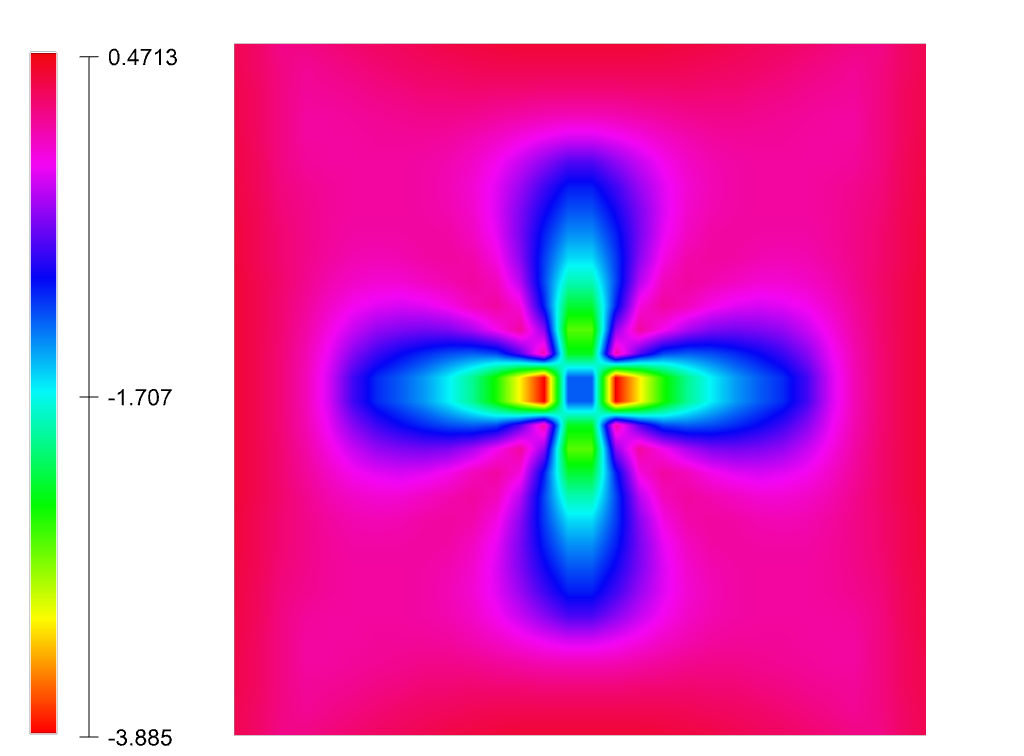
(a) $\lambda_{\max}$

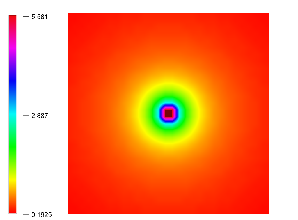
(b) $\lambda_{\max}$

Figure 2: Major eigenvalue the incorrect (left) and correct (right row) viscosity, shown along the XZ plane.

The tensor field is symmetric and of rank two, however it is not positive definite and may exhibit vanishing trace. The correct TAV is trace-free in the entire domain, whereas the trace of the incorrect TAV ranges through positive values (for large radial distances) to large negative values close to the coordinate origin, as depicted in Fig. 3 .

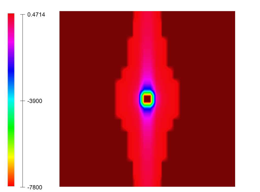
(a) $\mathrm{Tr}\mathbf{Q}_{\text{incorr}}$

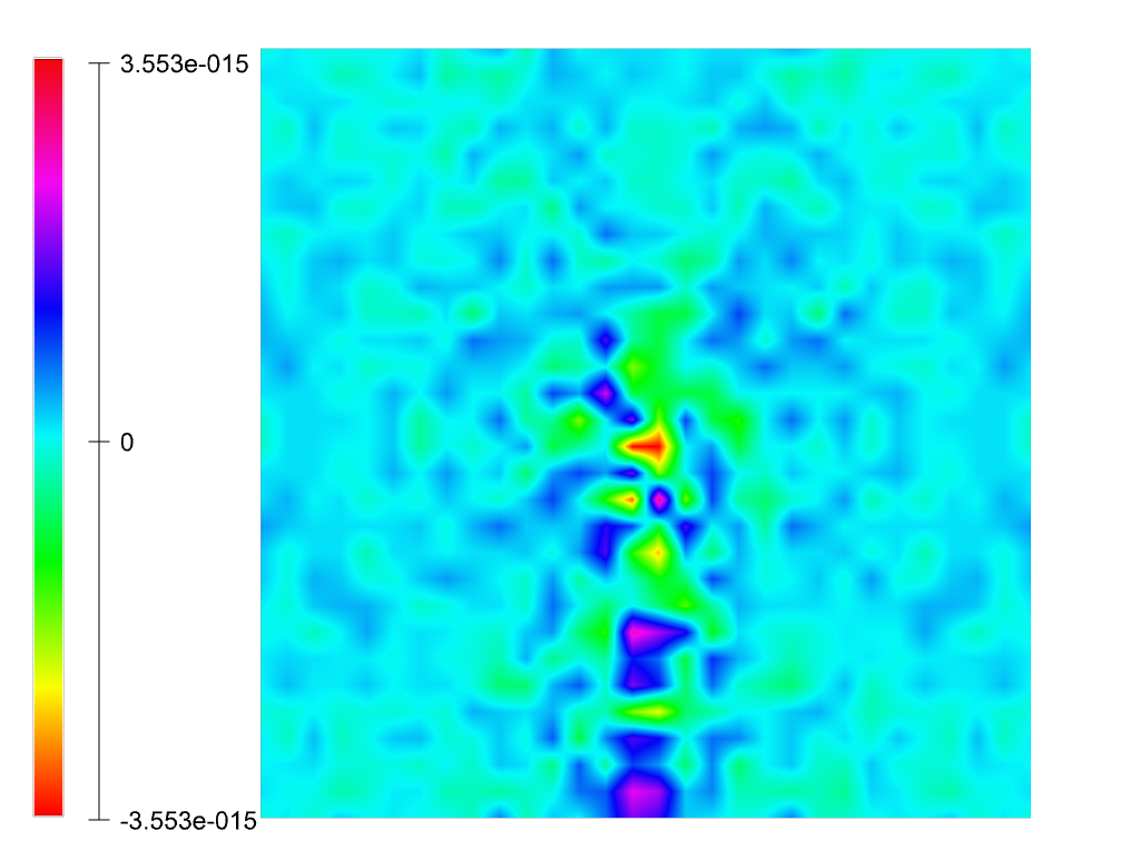
(b) $\mathrm{Tr}\mathbf{Q}_{\text{corr}}$

Figure 3: Trace the incorrect (left) and correct (right row) viscosity, shown along the XZ plane. Note the range of values in Fig. 3(b) - what we see is just numerical noise, the trace is perfectly zero within numerical precision.

A direct visualization method depicting the full six-dimensional degrees of freedom the tensor field is thus favorable, or even rather essential. However, many direct visualization methods for tensor fields require positive definiteness and are thus not applicable to this data. Only very few methods are suitable for general tensors. Fig. 4 shows so-called Reynold glyphs (Moore et al., 1995) for the TAV field. A Reynold glyph is the surface generated by mapping a tangential vector $v(P)$ at each data sample point $P$ as

$$P\rightarrow Q\left(v(P),v(P)\right).$$

Such glyphs shown at each sampling point provide a direct visualization of the full six-dimensional degrees of freedom of the tensor properties. Reynold glyphs are able to also depict negative definite tensors, whereas a quadric surface (ellipsoids representing $P\rightarrow 1/\sqrt{Q\left(v(P),v(P)\right)}$ becomes hyperbolic for negative eigenvalues and problematic for visualization purposes. The Reynold glyph directly show the “directional value” $Q\left(v(P),v(P)\right)$ of the tensor field $Q$ in the direction $v$ around a the sampling point $P$ - the resulting surface is intersecting the sampling point $P$ whenever $Q\left(v(P),v(P)\right)=0$, which is the case for points where the tensor is degenerating and not positive definite. In such areas the glyph will visually appear like two intersecting surfaces corresponding to the isopotential surfaces of second order spherical harmonic functions. These both surface components represent positive and negative eigenvalues of the tensor field - if both positive and negative component “counter-balance” themselves they therefore indicate vanishing trace, which is the sum of the eigenvalues. If only one surface component is visible, then the tensor is either positive or negative definite on that certain point.

We used a radial sampling for the direct visualization of the tensor field in order to minimize coordinate artificats. As depicted in Fig. 4(b) and Fig. 5(b) for the correct TAV all “modes” are equivalently represented, indicating vanishing trace of the tensor field while being radially aligned with the underlying coordinate system. In contrast, the incorrect TAV, Fig. 4(a) and Fig. 5(a), exhibits a dominantly negative trace.

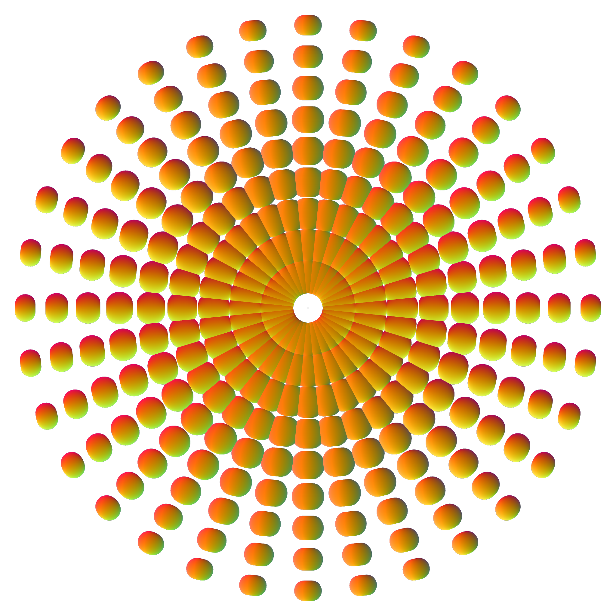
(a) Incorrect

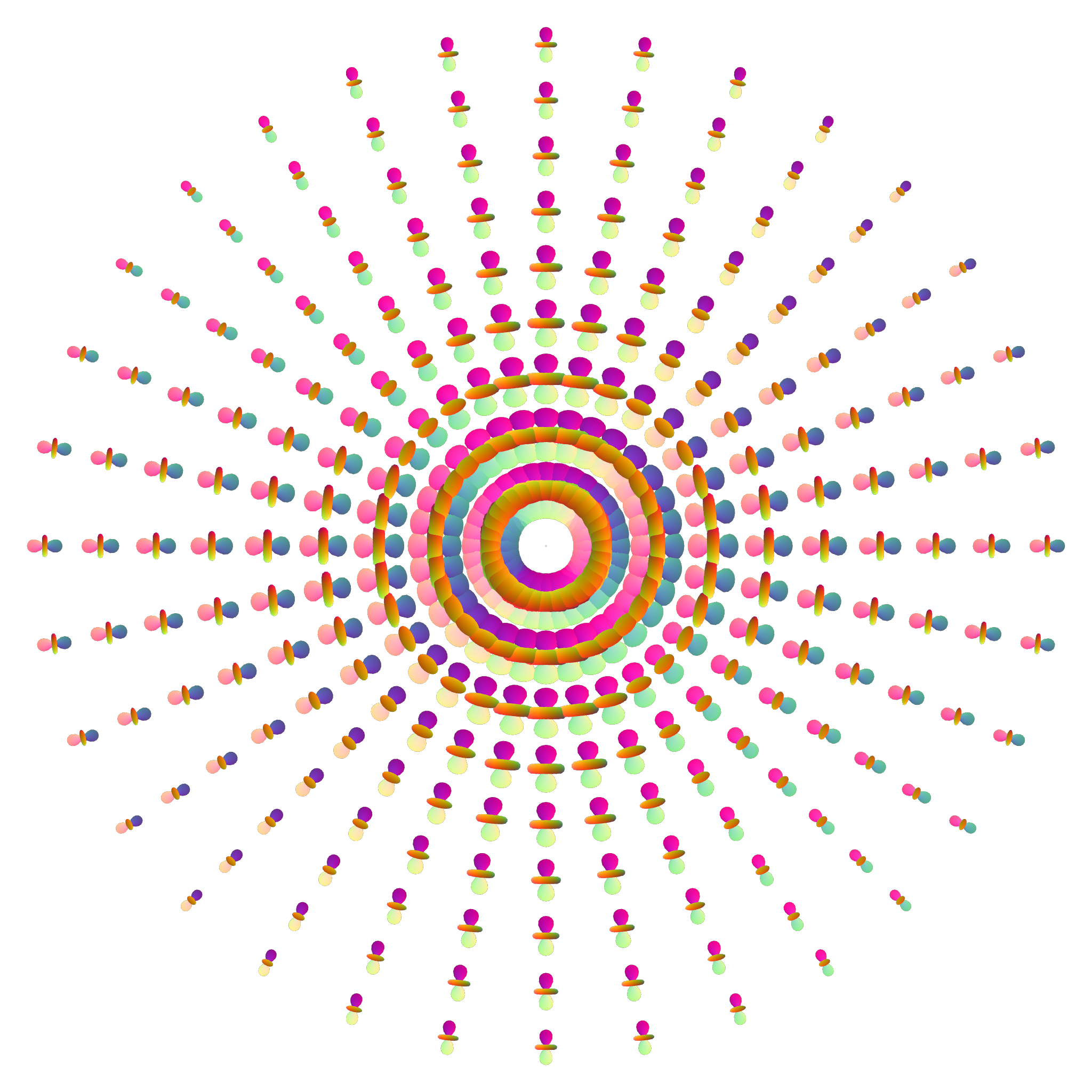
(b) Correct

Figure 4: Reynold glyphs (Moore et al., 1995) of the incorrect and correct viscosity tensor. The incorrect tensor showing a strongly negative component, whereas the correct tensor is balanced, indicating zero trace.

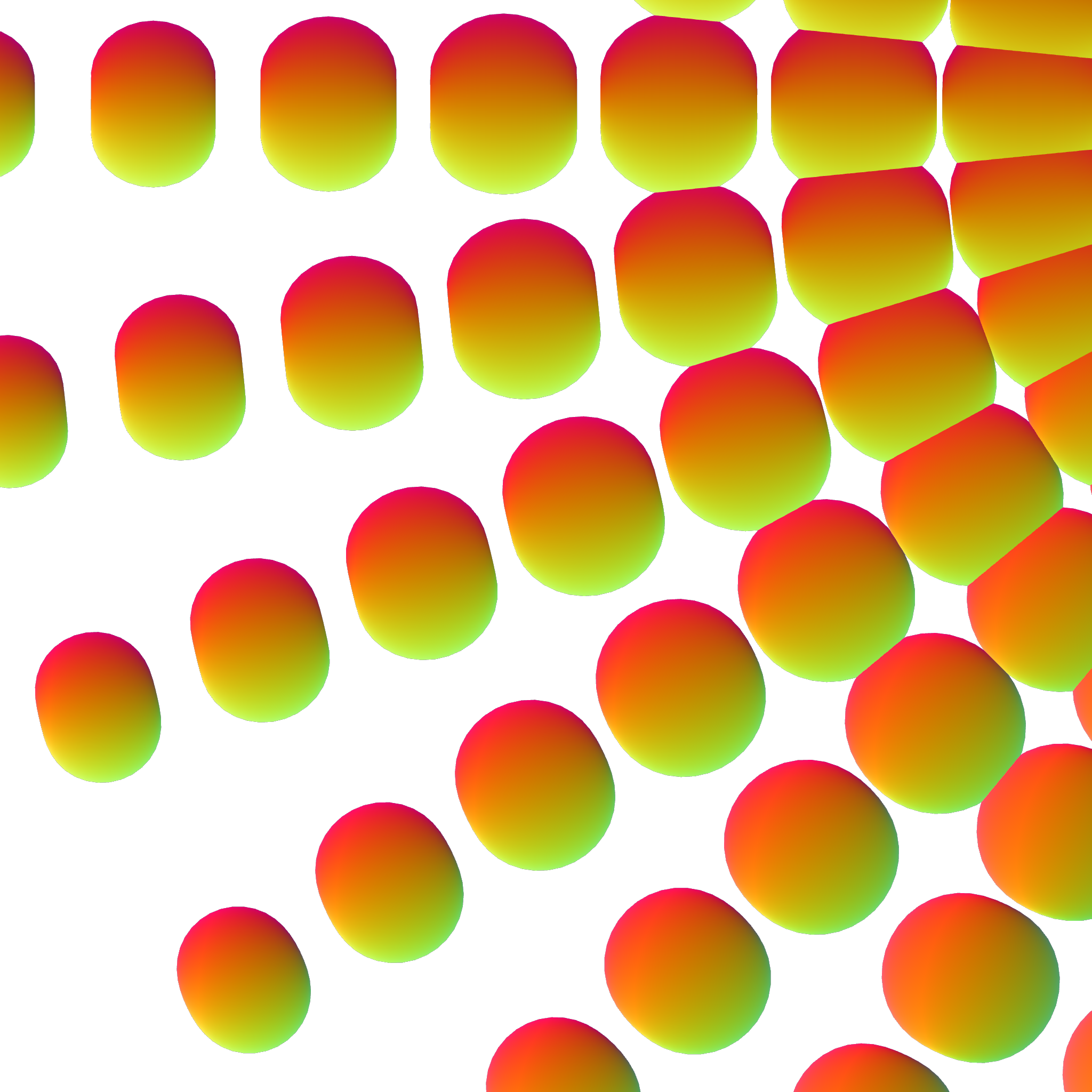
(a) Detail of the incorrect viscosity

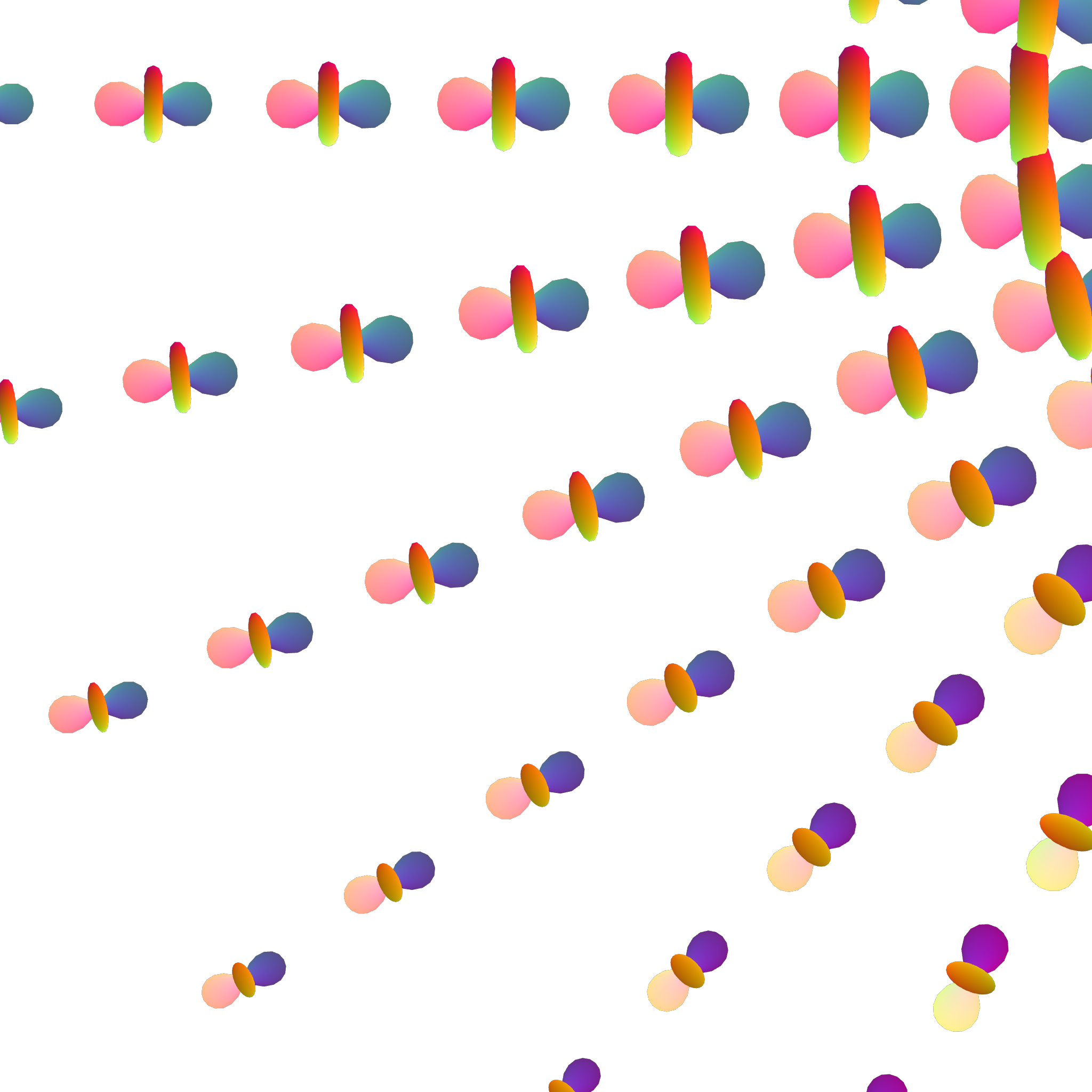
(b) Detail of the correct viscosity

Figure 5: Detailed Reynold glyphs (Moore et al., 1995) of the incorrect and correct viscosity tensor. Glyphs of the correct tensor show spherical harmonics that are balanced in their positive and negative half-widths.

4 Conclusions

We studied a generalization of the tensor of numerical artificial viscosity for curvilinear coordinates and compared our result to previous definitions found in literature. We analyzed a symmetric toy velocity field and visualized its viscosities. Clearly, the non-metric version of the TAV as used by many authors of hydro- (HD) respectively magneto-hydro- (MHD) or radiation hydrodynamic-codes (RHD) leads to incorrect results in curvilinear coordinates, whereas our suggestion for the numerical artificial viscosity gives geometrically consistent results.

5 Appendix

As mentioned in section 1, the benefit of the strong formulation of Cauchy problems arising from physical conservation laws will be discussed in more detail here.

Following the ideas of  (Warsi, 1981), in non-steady coordinates the geometrically consistent strong form of tensorial conservation laws (2) is given as

$$\partial_{t}\left(\sqrt{|\mathbf{g}|}\,\mathbf{d}\right)+\partial_{i}\left(\sqrt{|\mathbf{g}|}\,\mathbf{f}(\mathbf{d})\cdot\mathbf{{e}}^{i}\right)=0,$$ (22)

where $\mathbf{d}$ and $\mathbf{f}$ are to be decomposed according to their native tensorial components. The scalar multiplication with the $i$-th contravariant base vectors $\mathbf{{e}}^{i}$ yields a projection on the contravariant coordinate lines which in case of generalized grids can differ in direction and length of their covariant counterparts. Equation (22) gives also the integral form of the conservation law, which should be treated numerically in a correct way for non-steady coordinates in any finite-volume discretization. The important difference to the componentwise structure $\nabla(.)=\partial(.)+\Gamma(.)$, where Christoffel symbols account for the geometry is that in this case undifferentiated terms arise (see  (Marcel and Vinokur, 1974)) which act like geometric sources in the equations and destroy conservativeness. A comprehensive proof of Vinokurs theorem using differential forms can be found in  (Bridges, 2008).

With non-steady curvilinear grids not only the nonlinearity of the metric tensor but also its time-dependence has to be taken into account numerically. The motion of the grid itself and its implications on the formulation of the set of equations respectively the calculation of the occurring fluxes is discussed in the following section.

5.1 Adaptive Grids

In fluid dynamics we distinguish two main reference systems that suit unequally for various applications. The Eulerian frame is the fixed reference system of an external observer in which the fluid moves with velocity $\mathbf{u}$ whereas the Lagrangian approach describes the physics in the rest frame of the fluid. Between these two systems, the transformation of an advection term for a density $\mathbf{d}$ (that moves with a relative velocity $\mathbf{u}$) is given via the material derivative $D_{t}\mathbf{d}=\partial_{t}\mathbf{d}+\mathbf{u}\cdot\nabla\mathbf{d}$.

Hence, when we work with comoving frames, the coordinate system respectively the computational grid is time-dependent. There is a number of purposes where strict Eulerian or Lagrangian grids are suboptimal and thus we need to consider the generalized the concept of the comoving frames.

We want to evolve the strong conservation form for time dependent general coordinate systems. The time derivative of a density $\mathbf{d}$ in the coordinate system $\Sigma_{(\beta)}$ relative to a (e.g. static) coordinate system $\Sigma_{(\alpha)}$ is given by ${\partial_{t}\mathbf{d}}_{(\beta)}={\partial_{t}\mathbf{d}}_{(\alpha)}+\mathbf{\nabla}_{(\alpha)}\mathbf{d}\,{\partial_{t}\mathbf{x}}_{(\beta)}$ and from the view point of system $\Sigma_{(\alpha)}$, the time derivative is given as

$${\partial_{t}\mathbf{d}}_{(\alpha)}={\partial_{t}\mathbf{d}}_{(\beta)}-\dot{\mathbf{x}}\cdot\mathbf{\nabla}_{(\alpha)}\mathbf{d}^{\mathrm{T}},$$ (23)

where $\dot{\mathbf{x}}$ denotes the grid velocity. The second term on the right side we call grid advection, see e.g.  (Warsi, 1981) and  (Thompson et al., 1985). An inhomogeneous advective term of a conservation law $\mathbf{K}=\mathbf{d}_{t}+\mathrm{div}\,(\mathbf{u}^{\mathrm{T}}\mathbf{d})$ (in a fixed coordinate system) is given in the case of moving grid as

$$\mathbf{K}=\mathbf{d}_{t}-\dot{\mathbf{x}}\cdot\mathbf{\nabla}\mathbf{d}^{\mathrm{T}}+\mathrm{div}\,(\mathbf{u}^{\mathrm{T}}\mathbf{d}).$$ (24)

When we apply the appropriate transformation prescriptions to the spatial derivatives, we gain the following form

$$\mathbf{K}=\mathbf{d}_{t}-\dot{\mathbf{x}}\cdot\frac{1}{\sqrt{|\mathbf{g}|}}\partial_{i}\left(\sqrt{|\mathbf{g}|}\mathbf{{e}}^{i}\mathbf{d}\right)+\frac{1}{\sqrt{|\mathbf{g}|}}\partial_{i}\left(\sqrt{|\mathbf{g}|}\mathbf{u}\cdot\mathbf{{e}}^{i}\mathbf{d}\right).$$ (25)

Now this is not yet geometrically conservative, since it is not of an integral structure. Following the idea of the Reynolds transport theorem we consider the temporal derivative of the volume respectively the determinant of the time dependent metric tensor $\sqrt{|\mathbf{g(\mathbf{x},t)}|}$ in order to study the conservation of a density function in variable volumes and obtain the strong conservation form for time dependent coordinate systems:

$$\sqrt{|\mathbf{g}|}\mathbf{K}=\partial_{t}\left(\sqrt{|\mathbf{g}|}\mathbf{d}\right)+\partial_{i}\left(\sqrt{|\mathbf{g}|}\mathbf{{{e}}}^{i}\cdot(\mathbf{u}-\dot{\mathbf{x}})\mathbf{d}\right)$$ (26)

For the full analytic derivation we refer to  (Thompson et al., 1985) again. Defining the contravariant velocity components relative to the moving grid by $U^{i}=\mathbf{{{e}}}^{i}\cdot(\mathbf{u}-\dot{\mathbf{x}})$ the above equations yield

$$\sqrt{|\mathbf{g}|}\mathbf{K}=\partial_{t}\left(\sqrt{|\mathbf{g}|}\mathbf{d}\right)+\partial_{i}\left(\sqrt{|\mathbf{g}|}U^{i}\mathbf{d}\right).$$ (27)

5.2 Set of RHD Equations in Strong Conservation Form

We exhibit the system of equations of radiation hydrodynamics in somewhat simplified formulation. The following system has been basis for a number of implicit RHD computations (see e.g. (Dorfi, 1999)). All the astrophysical assumptions, implications and simplifications can be found in (Mihalas and Mihalas, 1984). In this paper we only want to emphasize the structural form of such a set of equations in a strong conservation form for comoving curvilinear coordinates. Note that for scalar equations the only effectively remaining geometric term inside the derivatives is the volume element $\sqrt{|\mathbf{g}|}$. The vectorial equations contain however also the time dependent base vectors.

5.2.1 Continuity Equation

The strong conservation form of the continuity equation

$$\partial_{t}\rho+\mathrm{div}\,(\rho\mathbf{u})=0$$

is given for time depended coordinates by

$$\partial_{t}\left(\sqrt{|\mathbf{g}|}\rho\right)+\partial_{i}\left(\sqrt{|\mathbf{g}|}\mathbf{{{e}}}^{i}\cdot(\mathbf{u}-\dot{\mathbf{x}})\rho\right)=0.$$

5.2.2 Equation of Motion

The equation of motion that we consider in radiation hydrodynamics contains the conservation of moment of plain fluid dynamics (5), the radiative flux as a coupling term ($\mathbf{H}$, with the specific Rosseland opacity of the fluid $\kappa_{R}$), gravitational force ($\mathbf{G}$) and the artificial viscosity term ($\mathbf{Q}$ from (17)):

$$\partial_{t}(\rho\mathbf{u})+\mathrm{div}\,\big{(}\rho\mathbf{u}^{\mathrm{T}}\mathbf{u}+\mathbf{P}+{\mathbf{Q}}\big{)}+\rho\mathbf{G}-\frac{4\pi}{c}\kappa_{R}\rho\mathbf{H}=0.$$

We investigate the elements of the energy stress tensor a little closer before we give the consistent strong conservation form. We define an effective tensor of gaseous momentum $\mathbf{R}$ that accounts for the motion of the coordinates as

$$\mathbf{R}=r^{ij}\mathbf{{e}}_{i}\mathbf{{e}}_{j}=\rho(\mathbf{u}-\dot{\mathbf{x}})\,\mathbf{u}^{\mathrm{T}}.$$

The isotropic gas pressure tensor $\mathbf{P}$ is defined by the scalar pressure and the metric tensor as $\mathbf{P}=p\mathbf{g}$. The viscous pressure tensor ${\mathbf{Q}}$ is to be modified in the way we suggested in (17). Since in most applications of RHD with self-gravity involved, the gravitational force $\mathbf{G}$ is determined by solving the Poisson equation for the potential $\Phi$, we substitute $\mathbf{G}=-\nabla\Phi$. The equation of motion in strong conservation form is then written as

$$\partial_{t}\left(\sqrt{|\mathbf{g}|}\rho\mathbf{u}\right)+\partial_{i}\left(\sqrt{|\mathbf{g}|}\,\big{(}\mathbf{R}+\mathbf{P}+{\mathbf{Q}}\big{)}\cdot\mathbf{{{e}}}^{i}\right)\,+$$

$$+\,\rho\partial_{i}\left(\sqrt{|\mathbf{g}|}\Phi\mathbf{{e}}^{i}\right)-\frac{4\pi}{c}\kappa_{R}\sqrt{|\mathbf{g}|}\rho\mathbf{H}=0.$$

The $k$th component of the strong conservation equation of motion is given by the $k$th Cartesian component of the unit vector, e.g. in spherical coordinates $\mathbf{{{e}}}^{r}=\cos\varphi\sin\vartheta\mathbf{e}^{x}+\sin\varphi\sin\vartheta\mathbf{e}^{y}+\cos\vartheta\mathbf{e}^{z}$ and its derivatives. The projection of each physical tensor on the contravariant coordinate lines can be simplified by its contravariant components with respect to its covariant basis without losing strong conservation form, i.e. $\mathbf{f}\cdot\mathbf{e}^{i}=f^{i,j}\mathbf{e}_{j}$. We prefer this form with contravariant components since it meets the native design of the stress tensor $\mathbf{R}$ and the pressure tensor $\mathbf{P}$. The tensor of artificial viscosity as given in (18) is brought to contravariant form by the summation

$$Q^{ij}=Q_{lm}g^{li}g^{mj}=\dots=\left(g^{li}g^{mj}(\nabla_{l}u_{m}+\nabla_{j}u_{m})-g^{ij}\frac{1}{3}\mathrm{div}\,\mathbf{u}\right)$$

and then the equation of motion as

$$\partial_{t}\left(\sqrt{|\mathbf{g}|}\rho u^{i}\mathbf{{e}}_{i}\right)+\partial_{i}\left(\sqrt{|\mathbf{g}|}\left(r^{ij}+p^{ij}+Q^{ij}\right)\mathbf{{{e}}}_{j}\right)+$$ (28)

$$+\,\rho\partial_{i}\left(\sqrt{|\mathbf{g}|}\Phi\mathbf{{e}}^{i}\right)-\frac{4\pi}{c}\kappa_{R}\sqrt{|\mathbf{g}|}\rho H^{i}\mathbf{{e}}_{i}=0.$$

5.2.3 Equation of Internal Energy

The energy equation

$$\partial_{t}(\rho\epsilon)+\mathrm{div}\,(\mathbf{u}\rho\epsilon)+\mathbf{P}\cdot\nabla\mathbf{u}^{\mathrm{T}}-4\pi\kappa_{P}\rho(J-S)+\mathbf{Q}\cdot\nabla\mathbf{u}^{\mathrm{T}}=0$$

accounts for the thermodynamics of the fluid, namely the energy balance including kinetic and pressure parts as well as inner energy. Latter is a thermodynamic quantity which is associated with the equation of state. The specific inner energy ($\epsilon$) is in case of an ideal fluid its thermic energy. Another term comes from the energy exchange with the radiation field ($(J-S)$-term) containing the specific Planck opacity $\kappa_{P}$ and viscous energy dissipation, expressed by the contraction of the viscosity with the velocity gradient $\mathbf{Q}\cdot\nabla\mathbf{u}^{\mathrm{T}}$.

Since we assume isotropic gas pressure $\mathbf{P}=p\mathbf{g}$ we can reformulate its contribution via the Ricci Lemma and obtain a very simple scalar expression.

$$\mathbf{P}\cdot\nabla\mathbf{u}^{\mathrm{T}}=g^{ij}p\nabla_{i}u_{j}=p\nabla_{i}u^{i}=p\,\mathrm{div}\,\mathbf{u}$$

The viscous energy dissipation is given by the contraction

$$\mathbf{Q}\cdot\nabla\mathbf{u}^{\mathrm{T}}=Q^{ij}\nabla_{i}u_{j}=Q^{ij}\left(\partial_{i}u_{j}-{\Gamma^{k}}_{ij}u_{k}\right)=:\mathsf{E}_{\mathrm{diss}},$$

and the strong conservative form of the energy equation is then given by

$$\partial_{t}\left(\sqrt{|\mathbf{g}|}\rho\epsilon\right)+\partial_{i}\left(\sqrt{|\mathbf{g}|}\rho\epsilon\,\mathbf{{{e}}}^{i}\cdot(\mathbf{u}-\dot{\mathbf{x}})\right)+\sqrt{|\mathbf{g}|}p\,\mathrm{div}\,\mathbf{u}\,-$$

$$-\,4\pi\sqrt{|\mathbf{g}|}\kappa_{P}\rho(J-S)+\sqrt{|\mathbf{g}|}\mathsf{E}_{\mathrm{diss}}=0.$$

5.2.4 Equation of Radiation Energy

We write a simplified frequency integrated radiation energy equation in the comoving frame as follows

$$\partial_{t}J+\mathrm{div}\,(\mathbf{u}J)+c\,\mathrm{div}\,\mathbf{H}+\mathbf{K}\cdot\nabla\mathbf{u}^{\mathrm{T}}+c\chi_{P}(J-S)=0.$$

For the scalar energy input of radiative pressure into the material we define a new coupling variable

$$\mathbf{K}\cdot\nabla\mathbf{u}^{\mathrm{T}}=K^{ij}\nabla_{i}u_{j}=:\mathsf{P}_{\mathrm{coup}}$$

and in strong conservation form the equation of radiation energy is given by

$$\partial_{t}\left(\sqrt{|\mathbf{g}|}J\right)+\partial_{i}\left(\sqrt{|\mathbf{g}|}\,\mathbf{{{e}}}^{i}\cdot\left(J(\mathbf{u}-\dot{\mathbf{x}})+c\mathbf{H}\right)\right)+$$

$$+\,\sqrt{|\mathbf{g}|}\mathsf{P}_{\mathrm{coup}}+\sqrt{|\mathbf{g}|}c\chi_{P}(J-S)=0.$$

5.2.5 Radiative Flux Equation

Another vectorial conservation law, the radiative flux equation, remains to be written:

$$\partial_{t}\mathbf{H}+\mathrm{div}\,(\mathbf{u}\mathbf{H})+c\,\mathrm{div}\,\mathbf{K}+\mathbf{H}\cdot\nabla\mathbf{u}^{\mathrm{T}}+c\chi_{R}\mathbf{H}=0.$$

We define an effective radiative flux tensor $\mathbf{L}$ analogously to the effective tensor of gaseous momentum:

$$(\mathbf{u}-\dot{\mathbf{x}})\mathbf{H}=:\mathbf{L}=l^{ij}\mathbf{{e}}_{i}\mathbf{{e}}_{j}$$

and for the contribution of radiative momentum to the material $\mathbf{H}\cdot\nabla\mathbf{u}^{\mathrm{T}}$ we define another coupling variable $\mathsf{F}$ with components

$$\mathsf{F}_{\mathrm{coup}}^{j}=H^{i}\nabla_{i}u^{j}.$$

The geometrically conservative form of the radiative flux equation in non-steady coordinates is then written as

$$\partial_{t}\left(\sqrt{|\mathbf{g}|}\mathbf{H}\right)+\partial_{i}\left(\sqrt{|\mathbf{g}|}\,\mathbf{{{e}}}^{i}\cdot\left(\mathbf{L}+c\mathbf{K}\right)\right)+$$

$$+\,\sqrt{|\mathbf{g}|}\mathsf{F}_{\mathrm{coup}}+\sqrt{|\mathbf{g}|}\kappa_{R}\rho\mathbf{H}=0.$$

5.3 Acknowledgements

We thank Franz Embacher and Helmuth Urbantke for valuable discussions on tensor analysis and differential geometry. The authors acknowledge the UniInfrastrukturprogramm des BMWF Forschungsprojekt Konsortium Hochleistungsrechnen, the Forschungsplattform Scientific Computing at LFU Innsbruck and the doctoral school - Computational Interdisciplinary Modelling FWF DK-plus (W1227). This research employed resources of the Center for Computation and Technology at Louisiana State University, which is supported by funding from the Louisiana legislature’s Information Technology Initiative.

References

- (1)
- Benger et al. (2007) Benger, W., Ritter, G. and Heinzl, R. (2007). The Concepts of VISH, High-End Visualization Workshop, Obergurgl, Tyrol, Austria, June 18-21, 2007, Berlin, Lehmanns Media-LOB.de, pp. 26–39.
-
Benson and Schoenfeld (1993)
Benson, D. J. and Schoenfeld, S. (1993).
A total variation diminishing shock viscosity, Computational
Mechanics 11: 107–121.
10.1007/BF00350046.
http://dx.doi.org/10.1007/BF00350046 -
Bridges (2008)
Bridges, T. J. (2008).
Conservation laws in curvilinear coordinates: A short proof of
vinokur’s theorem using differential forms, Applied Mathematics and
Computation 202(2): 882 – 885.
http://www.sciencedirect.com/science/article/B6TY8-4RXJYK5-1/2/cc34b069dcd4d9e9c2a854055c8bceec -
Dorfi (1999)
Dorfi, E. A. (1999).
Implicit radiation hydrodynamics for 1d-problems, Journal of
Computational and Applied Mathematics 109(1-2): 153 – 171.
http://www.sciencedirect.com/science/article/pii/S0377042799001570 -
Fryxell et al. (2000)
Fryxell, B., Olson, K., Ricker, P., Timmes, F. X., Zingale, M., Lamb, D. Q.,
MacNeice, P., Rosner, R., Truran, J. W. and Tufo, H.
(2000).
Flash: An adaptive mesh hydrodynamics code for modeling astrophysical
thermonuclear flashes, The Astrophysical Journal Supplement Series 131(1): 273.
http://stacks.iop.org/0067-0049/131/i=1/a=273 - Godlewski and Raviart (1992) Godlewski, E. and Raviart, P. (1992). Numerical approximation of hyperbolic systems of conservation laws, Applied Mathematica Sciences 18(18).
-
Harten et al. (1976)
Harten, A., Hyman, J. M., Lax, P. D. and Keyfitz, B. (1976).
On finite-difference approximations and entropy conditions for
shocks, Communications on Pure and Applied Mathematics 29(3): 297–322.
http://dx.doi.org/10.1002/cpa.3160290305 -
Iwakami et al. (2008)
Iwakami, W., Ohnishi, N., Kotake, K., Yamada, S. and Sawada, K.
(2008).
Numerical methods for three-dimensional analysis of shock instability
in supernova cores, Journal of Physics: Conference Series 112(4): 042021.
http://stacks.iop.org/1742-6596/112/i=4/a=042021 - Landshoff (1955) Landshoff, R. (1955). A numerical method for treating fluid flow in the presence of shocks, Los Alamos National Laboratory Report LA-1930.
- Lax and Wendroff (1960) Lax, P. and Wendroff, B. (1960). Systems of conservation laws, Communications on Pure and Applied Mathematics 13(2).
-
LeVeque (1991)
LeVeque, R. (1991).
Numerical methods for conservation laws, Mathematics and
Computers in Simulation 33(2): 180 – 180.
Birkhaeuser, Basel, 1990. 214 pp. (paperback), SFR.38, ISBN
3-7643-2464-3.
http://www.sciencedirect.com/science/article/B6V0T-48CX3P8-R/2/f5d635c435cb76407c78b23338bd7c11 -
Marcel and Vinokur (1974)
Marcel and Vinokur (1974).
Conservation equations of gasdynamics in curvilinear coordinate
systems, Journal of Computational Physics 14(2): 105 – 125.
http://www.sciencedirect.com/science/article/pii/0021999174900084 - Mignone et al. (2007) Mignone, A., Bodo, G., Massaglia, S., Matsakos, T., Tesileanu, O., Zanni, C. and Ferrari, A. (2007). Pluto: A numerical code for computational astrophysics, apjs 170: 228–242.
- Mihalas and Mihalas (1984) Mihalas, D. and Mihalas, B. W. (1984). Foundations of Radiation Hydrodynamics, Oxford University Press.
-
Moore et al. (1995)
Moore, J., Schorn, S. and Moore, J. (1995).
Methods of classical mechanics applied to turbulence stresses in a
tip leakage vortex, Journal of Turbomachinery 118(95-GT-220).
http://www.sv.vt.edu/classes/ESM4714/methods/EEG.html - Pons et al. (2000) Pons, J. A., Ibanez, J. M. and Miralles, J. A. (2000). Hyperbolic character of the angular moment equations of radiative transfer and numerical methods, Monthly Notices of the Royal Astronomical Society 317(3): 550–562.
- Richtmyer and Morton (1994) Richtmyer, R. D. and Morton, K. W. (1994). Difference Methods for Initial-Value Problems, Krieger Pub Co.
- Thompson et al. (1985) Thompson, J. F., Warsi, Z. U. and Mastin, C. W. (1985). Numerical grid generation: foundations and applications, Elsevier North-Holland, Inc., New York, NY, USA.
-