Lagrangian cobordism and Fukaya categories

1. Introduction

The purpose of this paper is to show that geometric Lagrangian cobordisms translate algebraically, in a functorial way, into iterated triangular decompositions in the derived Fukaya category.

Fix a symplectic manifold $M$ as well as a class $\mathcal{L}$ of Lagrangian submanifolds of $M$ (the precise class will be made explicit in §2.1). Floer homology, introduced in Floer’s seminal work [Flo] and extended in subsequent works [Oh1, FOOO1, FOOO2], associates to a pair of Lagrangians $L,L^{\prime}$ in our class a $\mathbb{Z}_{2}$-vector space $HF(L,L^{\prime})$. Assuming for the moment that $L$ is transverse to $L^{\prime}$, this is the homology of a chain complex $CF(L,L^{\prime})$, called the Floer complex, whose generators are the intersection points of $L$ and $L^{\prime}$. The differential counts “strips” $u:\mathbb{R}\times[0,1]\to M$ that join these intersection points, have boundaries along $L$ and $L^{\prime}$ and satisfy a Cauchy-Riemann type equation $\overline{\partial}_{J}u=0$ with respect to an almost complex structure $J$ on $M$ which is compatible with the symplectic structure. The fact that for generic $J$ such $J$-holomorphic curves form well-behaved moduli spaces originates in the fundamental work of Gromov [Gro] (see [MS2] for the foundations of the theory). The Floer complex thus depends on additional choices, in particular on $J$, however its homology $HF(L,L^{\prime})$ is invariant. Floer homology together with other additional structures, also based on counting $J$-holomorphic curves, are central tools in symplectic topology with wide-reaching applications.

In what Lagrangian topology is concerned, the most efficient way to aggregate these structures is provided by the derived Fukaya category whose definition we now sketch - a rigorous, detailed treatment that serves as foundation for our paper is contained in Seidel’s book [Sei3] - see also §2.5. Given a third Lagrangian $L^{\prime\prime}$ in our class, there is a product, due to Donaldson: $CF(L,L^{\prime})\otimes CF(L^{\prime},L^{\prime\prime})\to CF(L,L^{\prime\prime})$. This is defined by counting $J$-holomorphic triangles whose edges are mapped to $L$, $L^{\prime}$ and $L^{\prime\prime}$. This operation descends to homology where it is associative. It is therefore possible to define a category, called the Donaldson category of $M$, whose objects are the Lagrangians in $\mathcal{L}$ and with morphisms ${\textnormal{Mor\/}}_{Don}(L,L^{\prime})=HF(L,L^{\prime})$. The composition of morphisms is given by the triangle product. It was discovered by Fukaya [Fuk1, Fuk2] that, by taking into account the chain level data involving moduli spaces of $J$-holomorphic polygons with arbitrary number of edges, one can define a much richer algebraic structure, nowadays called the Fukaya $A_{\infty}$-category, $\mathcal{F}uk(M)$. The objects are the same as those of the Donaldson category, however, this is no longer a category in the classical sense (bur rather an $A_{\infty}$-category) because the triangle product is not associative at the chain level. Moreover, while the data contained in the Fukaya $A_{\infty}$-category is extremely rich, working directly with this $A_{\infty}$-category itself is quite difficult. Kontsevich [Kon] discovered that there is a triangulated completion of the Donaldson category to a true category called the derived Fukaya category and denoted by $D\mathcal{F}uk(M)$. Moreover, the derived Fukaya category is independent of the auxiliary structures used to define it up to appropriate equivalences and some of the finer information present at the level of $\mathcal{F}uk(M)$ survives the passage to $D\mathcal{F}uk(M)$.

Starting from the Fukaya $A_{\infty}$-category, the construction of $D\mathcal{F}uk(M)$ is algebraic, based on the fact that at the $A_{\infty}$-level it is possible to define cone-attachments (or in a different terminology, exact triangles) by a formula similar to the definition of the cone over a chain map in classical homological algebra. As a consequence, the triangulated structure of the derived category is somewhat mysterious and non-geometric in its definition. At the same time, it is precisely this triangulated structure that is often useful in the study of the Lagrangian submanifolds of $M$.

Lagrangian cobordism was introduced by Arnold [Arn1, Arn2], see also §2.2 for the specific variant used here. Consider one such cobordism

$$(V;L_{1}\cup\ldots\cup L_{k},L)~{}.~{}$$

This is a Lagrangian submanifold of $V\subset\mathbb{R}^{2}\times M$ with $k+1$-cylindrical ends so that there are $k$ negative ends, each identified with $(-\infty,0]\times\{i\}\times L_{i}$, $i=1,\ldots,k$, and one positive end identified with $[1,\infty)\times\{1\}\times L$. The projection of such a cobordism to $\mathbb{R}^{2}$ is like in Figure 1.

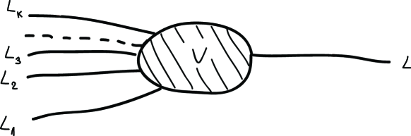
Figure 1. A cobordism $V\subset\mathbb{R}^{2}\times M$ with a single positive end $L$ and multiple negative ends $L_{1},\ldots,L_{k}$ projected on $\mathbb{R}^{2}$.

Of course, we will have to further restrict the class of Lagrangian cobordisms, the relevant constraints coming from the class $\mathcal{L}$ of Lagrangian submanifolds of $M$ that we have already fixed. We denote the class of admissible cobordisms by $\mathcal{L}_{cob}$. Its precise definition will be given in §2.3.

In this paper we establish the following fundamental correspondence between cobordism and the triangulated structure of the derived Fukaya category:

Theorem A.

If $V$ is a Lagrangian cobordism as above, then there exist $k$ objects $Z_{1},\ldots,Z_{k}$ in $D\mathcal{F}uk(M)$ with $Z_{1}=L_{1}$ and $Z_{k}\simeq L$ which fit into $k-1$ exact triangles as follows:

$$L_{i}[1]\to Z_{i-1}\to Z_{i}\to L_{i},\ \forall\,2\leq i\leq k.$$

In particular, $L$ belongs to the triangulated subcategory of $D\mathcal{F}uk(M)$ generated by $L_{1},L_{2},\ldots,L_{k}$.

The notation $L_{i}[1]$ stands for a shift by one in the grading for the object $L_{i}$. In fact we will work in an ungraded setting (thus $L_{i}[1]$ is the same as $L_{i}$). We left the grading shift in the notation, only in order to indicate the expected statement in the graded framework.

The first indication that a result like Theorem A holds appeared in [BC2] where we showed that for any fixed $N\in\mathcal{L}$, the Floer complexes

$$CF(N,L_{1}),\ldots,CF(N,L_{i}),\ldots,CF(N,L_{k}),CF(N,L)$$

fit into a sequence of chain cone-attachments as implied by Theorem A.

We deduce Theorem A as an immediate consequence of a stronger result, conjectured in [BC2], that provides a more complete and conceptual description of the relationship between cobordisms and triangulations. In particular, we will see that not only cobordisms provide triangular decompositions but, moreover, concatenation of cobordisms corresponds to refinement of the respective decompositions. More elaboration is needed to formulate this stronger result more precisely.

We use a category $\mathcal{C}ob(M)$ from [BC2]. We remark that an alternative, somewhat different categorical point of view on Lagrangian cobordism has been independently introduced by Nadler and Tanaka in [NT].

The objects of $\mathcal{C}ob(M)$ are finite ordered families of Lagrangian submanifolds of $M$ that belong to the class $\mathcal{L}$. The morphisms are isotopy classes of certain Lagrangian cobordisms, possibly multi-ended. (Again, the precise definitions are given in §2.3.) In particular, the cobordism $V$ considered earlier represents such a morphism.

The geometric category $\mathcal{C}ob(M)$ is monoidal under (essentially) disjoint union but is not triangulated. To relate the morphisms in $\mathcal{C}ob(M)$ to the triangular decompositions in $D\mathcal{F}uk(M)$ we consider a category $T^{S}D\mathcal{F}uk(M)$ that is obtained from $D\mathcal{F}uk(M)$ by a general construction, introduced in [BC2] and further detailed in §2.6, that associates to any triangulated category $\mathcal{C}$ a new category $T^{S}\mathcal{C}$ that is monoidal and whose morphisms sets, $\hom(x,-)$, parametrize the ways in which $x$ can be resolved by iterated exact triangles. The main purpose of $T^{S}D\mathcal{F}uk(M)$ is to encode the triangular decompositions in $D\mathcal{F}uk(M)$ as morphisms in a category that can serve as target to a functor defined on $\mathcal{C}ob(M)$.

Here is the main result of the paper.

Theorem B.

There exists a monoidal functor

$$\widetilde{\mathcal{F}}:\mathcal{C}ob(M)\longrightarrow T^{S}D\mathcal{F}uk(M),$$

with the property that $\widetilde{\mathcal{F}}(L)=L$ for every Lagrangian submanifold $L\in\mathcal{L}$.

Given that $V$ represents a morphism in $\mathcal{C}ob(M)$, Theorem A follows immediately from Theorem B and the definition of $T^{S}(-)$, the sequence of exact triangles in the statement being provided by $\widetilde{\mathcal{F}}(V)$.

Organization of the paper

The plan for the rest of the paper is as follows:  §2 contains extensive prerequisites, most importantly the basic cobordism definitions in §2.2, a short review in §2.5 of the construction of the Fukaya $A_{\infty}$-category basically following [Sei3] and, in §2.6, the definition of the category $T^{S}(-)$. Additionally, for completeness, in Appendix A we recall basic $A_{\infty}$-category notions. In §3 we set up a Fukaya $A_{\infty}$-category whose objects are cobordisms in $\mathbb{R}^{2}\times M$. As it will be explained below, this is an essential step in the proof of Theorem B. It might also be of independent interest. The proof of Theorem B appears in §4.

In the remainder of the introduction we pursue with some more technical remarks and corollaries of Theorem B. We then summarize the main steps in the proof Theorem B.

We refer to [BC2] for more extensive background and examples of Lagrangian cobordisms.

1.1. Further context and Corollaries of Theorem B

To further outline the properties of the functor $\widetilde{\mathcal{F}}$ from Theorem B it is useful to consider the commutative diagram below.

(1) $$\begin{aligned} \lx@xy@svg{\hbox{\raise 0.0pt\hbox{\kern 23.81944pt\hbox{\ignorespaces\ignorespaces\ignorespaces\hbox{\vtop{\kern 0.0pt\offinterlineskip\halign{\entry@#!@&&\entry@@#!@\cr&\\&\\&\crcr}}}\ignorespaces{\hbox{\kern-20.46529pt\raise 0.0pt\hbox{\hbox{\kern 0.0pt\raise 0.0pt\hbox{\hbox{\kern 3.0pt\raise 0.0pt\hbox{$\textstyle{\mathcal{C}ob(M)\ignorespaces\ignorespaces\ignorespaces\ignorespaces\ignorespaces\ignorespaces\ignorespaces\ignorespaces}$}}}}}}}\ignorespaces\ignorespaces\ignorespaces\ignorespaces{}{\hbox{\lx@xy@droprule}}\ignorespaces\ignorespaces\ignorespaces{\hbox{\kern 33.60416pt\raise 6.61111pt\hbox{{}\hbox{\kern 0.0pt\raise 0.0pt\hbox{\hbox{\kern 3.0pt\hbox{\hbox{\kern 0.0pt\raise-3.61111pt\hbox{$\scriptstyle{\widetilde{\mathcal{F}}}$}}}\kern 3.0pt}}}}}}\ignorespaces{\hbox{\kern 47.81944pt\raise 0.0pt\hbox{\hbox{\kern 0.0pt\raise 0.0pt\hbox{\lx@xy@tip{1}\lx@xy@tip{-1}}}}}}{\hbox{\lx@xy@droprule}}{\hbox{\lx@xy@droprule}}\ignorespaces\ignorespaces\ignorespaces\ignorespaces{}{\hbox{\lx@xy@droprule}}\ignorespaces\ignorespaces\ignorespaces{\hbox{\kern-10.7639pt\raise-20.31166pt\hbox{{}\hbox{\kern 0.0pt\raise 0.0pt\hbox{\hbox{\kern 3.0pt\hbox{\hbox{\kern 0.0pt\raise-2.39166pt\hbox{$\scriptstyle{\mathcal{P}}$}}}\kern 3.0pt}}}}}}\ignorespaces{\hbox{\kern 0.0pt\raise-30.12332pt\hbox{\hbox{\kern 0.0pt\raise 0.0pt\hbox{\lx@xy@tip{1}\lx@xy@tip{-1}}}}}}{\hbox{\lx@xy@droprule}}{\hbox{\lx@xy@droprule}}{\hbox{\kern 47.81944pt\raise 0.0pt\hbox{\hbox{\kern 0.0pt\raise 0.0pt\hbox{\hbox{\kern 3.0pt\raise 0.0pt\hbox{$\textstyle{T^{S}D\mathcal{F}uk(M)\ignorespaces\ignorespaces\ignorespaces\ignorespaces}$}}}}}}}\ignorespaces\ignorespaces\ignorespaces\ignorespaces{}{\hbox{\lx@xy@droprule}}\ignorespaces\ignorespaces\ignorespaces{\hbox{\kern 78.7639pt\raise-20.31166pt\hbox{{}\hbox{\kern 0.0pt\raise 0.0pt\hbox{\hbox{\kern 3.0pt\hbox{\hbox{\kern 0.0pt\raise-2.39166pt\hbox{$\scriptstyle{\mathcal{P}}$}}}\kern 3.0pt}}}}}}\ignorespaces{\hbox{\kern 78.7639pt\raise-30.12332pt\hbox{\hbox{\kern 0.0pt\raise 0.0pt\hbox{\lx@xy@tip{1}\lx@xy@tip{-1}}}}}}{\hbox{\lx@xy@droprule}}{\hbox{\lx@xy@droprule}}{\hbox{\kern-23.81944pt\raise-40.62332pt\hbox{\hbox{\kern 0.0pt\raise 0.0pt\hbox{\hbox{\kern 3.0pt\raise 0.0pt\hbox{$\textstyle{S\mathcal{C}ob(M)\ignorespaces\ignorespaces\ignorespaces\ignorespaces\ignorespaces\ignorespaces\ignorespaces\ignorespaces}$}}}}}}}\ignorespaces\ignorespaces\ignorespaces\ignorespaces{}{\hbox{\lx@xy@droprule}}\ignorespaces\ignorespaces\ignorespaces{\hbox{\kern 34.09721pt\raise-35.23166pt\hbox{{}\hbox{\kern 0.0pt\raise 0.0pt\hbox{\hbox{\kern 3.0pt\hbox{\hbox{\kern 0.0pt\raise-2.39166pt\hbox{$\scriptstyle{\mathcal{F}}$}}}\kern 3.0pt}}}}}}\ignorespaces{\hbox{\kern 53.31409pt\raise-40.62332pt\hbox{\hbox{\kern 0.0pt\raise 0.0pt\hbox{\lx@xy@tip{1}\lx@xy@tip{-1}}}}}}{\hbox{\lx@xy@droprule}}{\hbox{\lx@xy@droprule}}\ignorespaces\ignorespaces\ignorespaces{}\ignorespaces\ignorespaces{\hbox{\lx@xy@drawline@}}\ignorespaces\ignorespaces\ignorespaces{\hbox{\kern 24.02217pt\raise-66.69832pt\hbox{{}\hbox{\kern 0.0pt\raise 0.0pt\hbox{\hbox{\kern 3.0pt\hbox{\hbox{\kern 0.0pt\raise-1.70833pt\hbox{$\scriptstyle{\mathcal{H}F_{N}}$}}}\kern 3.0pt}}}}}}\ignorespaces{\hbox{\kern 62.8472pt\raise-72.55617pt\hbox{\hbox{\kern 0.0pt\raise 0.0pt\hbox{\lx@xy@tip{1}\lx@xy@tip{-1}}}}}}\ignorespaces\ignorespaces{\hbox{\lx@xy@drawline@}}\ignorespaces{\hbox{\lx@xy@drawline@}}{\hbox{\kern 53.31409pt\raise-40.62332pt\hbox{\hbox{\kern 0.0pt\raise 0.0pt\hbox{\hbox{\kern 3.0pt\raise 0.0pt\hbox{$\textstyle{D\mathcal{F}uk(M)\ignorespaces\ignorespaces\ignorespaces\ignorespaces}$}}}}}}}\ignorespaces\ignorespaces\ignorespaces\ignorespaces{}{\hbox{\lx@xy@droprule}}\ignorespaces\ignorespaces\ignorespaces{\hbox{\kern 78.7639pt\raise-60.62332pt\hbox{{}\hbox{\kern 0.0pt\raise 0.0pt\hbox{\hbox{\kern 3.0pt\hbox{\hbox{\kern 0.0pt\raise-1.75pt\hbox{$\scriptstyle{\hom(N,-)}$}}}\kern 3.0pt}}}}}}\ignorespaces{\hbox{\kern 78.7639pt\raise-70.12332pt\hbox{\hbox{\kern 0.0pt\raise 0.0pt\hbox{\lx@xy@tip{1}\lx@xy@tip{-1}}}}}}{\hbox{\lx@xy@droprule}}{\hbox{\lx@xy@droprule}}{\hbox{\kern-3.0pt\raise-80.62332pt\hbox{\hbox{\kern 0.0pt\raise 0.0pt\hbox{\hbox{\kern 3.0pt\raise 0.0pt\hbox{$\textstyle{}$}}}}}}}{\hbox{\kern 62.8472pt\raise-80.62332pt\hbox{\hbox{\kern 0.0pt\raise 0.0pt\hbox{\hbox{\kern 3.0pt\raise 0.0pt\hbox{$\textstyle{(\mathcal{V},\times)}$}}}}}}}\ignorespaces}}}}\ignorespaces\end{aligned} \textstyle{\mathcal{C}ob(M)\ignorespaces\ignorespaces\ignorespaces\ignorespaces\ignorespaces\ignorespaces\ignorespaces\ignorespaces} \scriptstyle{\widetilde{\mathcal{F}}} \scriptstyle{\mathcal{P}} \textstyle{T^{S}D\mathcal{F}uk(M)\ignorespaces\ignorespaces\ignorespaces\ignorespaces} \scriptstyle{\mathcal{P}} \textstyle{S\mathcal{C}ob(M)\ignorespaces\ignorespaces\ignorespaces\ignorespaces\ignorespaces\ignorespaces\ignorespaces\ignorespaces} \scriptstyle{\mathcal{F}} \scriptstyle{\mathcal{H}F_{N}} \textstyle{D\mathcal{F}uk(M)\ignorespaces\ignorespaces\ignorespaces\ignorespaces} \scriptstyle{\hom(N,-)} \textstyle{(\mathcal{V},\times)} \textstyle{\mathcal{C}ob(M)\ignorespaces\ignorespaces\ignorespaces\ignorespaces\ignorespaces\ignorespaces\ignorespaces\ignorespaces} \scriptstyle{\widetilde{\mathcal{F}}} \scriptstyle{\mathcal{P}} \textstyle{T^{S}D\mathcal{F}uk(M)\ignorespaces\ignorespaces\ignorespaces\ignorespaces} \scriptstyle{\mathcal{P}} \textstyle{S\mathcal{C}ob(M)\ignorespaces\ignorespaces\ignorespaces\ignorespaces\ignorespaces\ignorespaces\ignorespaces\ignorespaces} \scriptstyle{\mathcal{F}} \scriptstyle{\mathcal{H}F_{N}} \textstyle{D\mathcal{F}uk(M)\ignorespaces\ignorespaces\ignorespaces\ignorespaces} \scriptstyle{\hom(N,-)} \textstyle{(\mathcal{V},\times)}$$

We explain next the ingredients in this diagram.

1.1.1. A simple version of $\widetilde{\mathcal{F}}$ and the top square in (1)

We describe here the functor $\mathcal{F}$, that appears in the middle row in Diagram (1). For this, we introduce another cobordism category, denoted $S\mathcal{C}ob(M)$, which is simpler than $\mathcal{C}ob(M)$. Its objects are Lagrangians in the class $\mathcal{L}$ and the morphisms relating two such objects, $L$ and $L^{\prime}$, are horizontal isotopy classes of cobordisms $V$ in $\mathcal{L}_{cob}$ (see Definitions 2.2.1 and 2.2.3) so that $L$ is the unique “positive” end and $L^{\prime}$ is the “top” negative end of $V$, as in Figure 1 (with $L^{\prime}=L_{k}$). There is a canonical functor $\mathcal{P}:\mathcal{C}ob(M)\to S\mathcal{C}ob(M)$ that associates to a family $(L_{1},\ldots,L_{k})$ the last Lagrangian in the family, $L_{k}$, and has a similar action on morphisms. Directly out of the definition of $T^{S}D\mathcal{F}uk(M)$ - see §2.6, there also is a projection functor $\mathcal{P}:T^{S}D\mathcal{F}uk(M)\to D\mathcal{F}uk(M)$ that again associates to each family of Lagrangians the last object in the family. The construction of $\widetilde{\mathcal{F}}$ implies that there is an induced functor $\mathcal{F}:S\mathcal{C}ob(M)\to D\mathcal{F}uk(M)$ which is the identity on objects and makes the top square in the Diagram (1) commutative.

As it will be seen in more detail in §4.8, the functor $\mathcal{F}$ has the advantage that it can be explicitly described on morphisms as follows. Fix a cobordism $V$ representing a morphism between $L$ and $L^{\prime}$ in $S\mathcal{C}ob(M)$. The class $\mathcal{F}([V])\in HF(L,L^{\prime})=\hom_{D\mathcal{F}uk}(L,L^{\prime})$ is the image of the unity in $HF(L,L)$ (induced by the fundamental class of $L$) through a morphism $\phi_{V}:HF(L,L)\to HF(L^{\prime},L)$ that is given by counting Floer strips in $\mathbb{R}^{2}\times M$ with boundary conditions along $V$ on one side and on $\gamma\times L$ on the other side, $\mathcal{F}([V])=\phi_{V}([L])$. Here $\gamma\subset\mathbb{R}^{2}$, $V$ are as in Figure 2 (again with $L^{\prime}=L_{k}$) where are also depicted the planar projections of the strips whose count provides the morphism $\phi_{V}$.

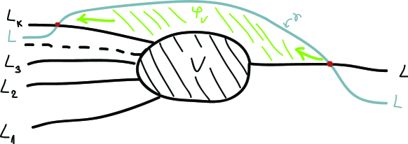
Figure 2. A cobordism $V\subset\mathbb{R}^{2}\times M$ with a positive end $L$ and with $L^{\prime}=L_{k}$ together with the projection of the $J$-holomorphic strips that define the morphism $\phi_{V}$.

Remark 1.1.1.

a. It has been verified by Charette-Cornea (§3.4 in [Cha]) that $\phi_{V}$ is an extension of the Lagrangian version of the Seidel morphism [Sei1] introduced by Hu-Lalonde [HL] (see also [Lec] and [HLL]) to which $\phi_{V}$ reduces when $V$ is the Lagrangian suspension associated to a Hamiltonian isotopy. Thus, from this perspective, Theorem B shows that the Seidel morphism extends to a natural correspondence $V\to\phi_{V}$ that satisfies the properties needed to define the functor $\mathcal{F}$.

b. In fact a stronger version of the remark at point a is true. It is proved in [CC] that the Seidel representation admits a categorification in the following sense: the fundamental groupoid of $Ham(M)$, $\Pi(Ham(M))$, viewed as a monoidal category, acts on both $\mathcal{C}ob(M)$ and $T^{S}D\mathcal{F}uk(M)$ and $\widetilde{\mathcal{F}}$ is equivariant with respect to this action.

We use the functor $\mathcal{F}$ to illustrate Theorem A in a particular case where we can also make the statement more precise by identifying the morphisms involved.

Corollary 1.1.2.

If the Lagrangian cobordism $(V;L_{1}\cup L_{2},L)$ has just two negative ends $L_{1},L_{2}\subset M$ (for instance, this happens if $L$ is obtained by surgery on $L_{1}$ and $L_{2}$ [BC2]), then there is an exact triangle in $D\mathcal{F}uk(M)$

(2) $$\begin{aligned} \lx@xy@svg{\hbox{\raise 0.0pt\hbox{\kern 23.85278pt\hbox{\ignorespaces\ignorespaces\ignorespaces\hbox{\vtop{\kern 0.0pt\offinterlineskip\halign{\entry@#!@&&\entry@@#!@\cr&&\\&&\\&&\crcr}}}\ignorespaces{\hbox{\kern-7.80278pt\raise 0.0pt\hbox{\hbox{\kern 0.0pt\raise 0.0pt\hbox{\hbox{\kern 3.0pt\raise 0.0pt\hbox{$\textstyle{L_{2}\ignorespaces\ignorespaces\ignorespaces\ignorespaces}$}}}}}}}\ignorespaces\ignorespaces\ignorespaces\ignorespaces{}{\hbox{\lx@xy@droprule}}\ignorespaces\ignorespaces\ignorespaces{\hbox{\kern-23.85278pt\raise-37.73553pt\hbox{{}\hbox{\kern 0.0pt\raise 0.0pt\hbox{\hbox{\kern 3.0pt\hbox{\hbox{\kern 0.0pt\raise-2.07222pt\hbox{$\scriptstyle{\mathcal{F}(V^{\prime\prime})}$}}}\kern 3.0pt}}}}}}\ignorespaces{\hbox{\kern 0.0pt\raise-65.63776pt\hbox{\hbox{\kern 0.0pt\raise 0.0pt\hbox{\lx@xy@tip{1}\lx@xy@tip{-1}}}}}}{\hbox{\lx@xy@droprule}}{\hbox{\lx@xy@droprule}}{\hbox{\kern 31.80278pt\raise 0.0pt\hbox{\hbox{\kern 0.0pt\raise 0.0pt\hbox{\hbox{\kern 3.0pt\raise 0.0pt\hbox{$\textstyle{}$}}}}}}}{\hbox{\kern 65.20557pt\raise 0.0pt\hbox{\hbox{\kern 0.0pt\raise 0.0pt\hbox{\hbox{\kern 3.0pt\raise 0.0pt\hbox{$\textstyle{}$}}}}}}}{\hbox{\kern-3.0pt\raise-37.73553pt\hbox{\hbox{\kern 0.0pt\raise 0.0pt\hbox{\hbox{\kern 3.0pt\raise 0.0pt\hbox{$\textstyle{}$}}}}}}}{\hbox{\kern 31.80278pt\raise-37.73553pt\hbox{\hbox{\kern 0.0pt\raise 0.0pt\hbox{\hbox{\kern 3.0pt\raise 0.0pt\hbox{$\textstyle{}$}}}}}}}{\hbox{\kern 61.80278pt\raise-37.73553pt\hbox{\hbox{\kern 0.0pt\raise 0.0pt\hbox{\hbox{\kern 3.0pt\raise 0.0pt\hbox{$\textstyle{L\ignorespaces\ignorespaces\ignorespaces\ignorespaces}$}}}}}}}\ignorespaces\ignorespaces\ignorespaces{}\ignorespaces\ignorespaces{\hbox{\lx@xy@drawline@}}\ignorespaces\ignorespaces\ignorespaces{\hbox{\kern 29.26051pt\raise-12.36777pt\hbox{{}\hbox{\kern 0.0pt\raise 0.0pt\hbox{\hbox{\kern 3.0pt\hbox{\hbox{\kern 0.0pt\raise-1.75pt\hbox{$\scriptstyle{\mathcal{F}(V)}$}}}\kern 3.0pt}}}}}}\ignorespaces{\hbox{\kern 7.8028pt\raise-4.31287pt\hbox{\hbox{\kern 0.0pt\raise 0.0pt\hbox{\lx@xy@tip{1}\lx@xy@tip{-1}}}}}}\ignorespaces\ignorespaces{\hbox{\lx@xy@drawline@}}\ignorespaces{\hbox{\lx@xy@drawline@}}{\hbox{\kern-7.80278pt\raise-75.47107pt\hbox{\hbox{\kern 0.0pt\raise 0.0pt\hbox{\hbox{\kern 3.0pt\raise 0.0pt\hbox{$\textstyle{L_{1}\ignorespaces\ignorespaces\ignorespaces\ignorespaces}$}}}}}}}\ignorespaces\ignorespaces\ignorespaces{}\ignorespaces\ignorespaces{\hbox{\lx@xy@drawline@}}\ignorespaces\ignorespaces\ignorespaces{\hbox{\kern 29.01453pt\raise-63.42552pt\hbox{{}\hbox{\kern 0.0pt\raise 0.0pt\hbox{\hbox{\kern 3.0pt\hbox{\hbox{\kern 0.0pt\raise-2.07222pt\hbox{$\scriptstyle{\mathcal{F}(V^{\prime})}$}}}\kern 3.0pt}}}}}}\ignorespaces{\hbox{\kern 62.78271pt\raise-40.73553pt\hbox{\hbox{\kern 0.0pt\raise 0.0pt\hbox{\lx@xy@tip{1}\lx@xy@tip{-1}}}}}}\ignorespaces\ignorespaces{\hbox{\lx@xy@drawline@}}\ignorespaces{\hbox{\lx@xy@drawline@}}{\hbox{\kern 31.80278pt\raise-75.47107pt\hbox{\hbox{\kern 0.0pt\raise 0.0pt\hbox{\hbox{\kern 3.0pt\raise 0.0pt\hbox{$\textstyle{}$}}}}}}}{\hbox{\kern 65.20557pt\raise-75.47107pt\hbox{\hbox{\kern 0.0pt\raise 0.0pt\hbox{\hbox{\kern 3.0pt\raise 0.0pt\hbox{$\textstyle{}$}}}}}}}\ignorespaces}}}}\ignorespaces\end{aligned} \textstyle{L_{2}\ignorespaces\ignorespaces\ignorespaces\ignorespaces} \scriptstyle{\mathcal{F}(V^{\prime\prime})} \textstyle{L\ignorespaces\ignorespaces\ignorespaces\ignorespaces} \scriptstyle{\mathcal{F}(V)} \textstyle{L_{1}\ignorespaces\ignorespaces\ignorespaces\ignorespaces} \scriptstyle{\mathcal{F}(V^{\prime})} \textstyle{L_{2}\ignorespaces\ignorespaces\ignorespaces\ignorespaces} \scriptstyle{\mathcal{F}(V^{\prime\prime})} \textstyle{L\ignorespaces\ignorespaces\ignorespaces\ignorespaces} \scriptstyle{\mathcal{F}(V)} \textstyle{L_{1}\ignorespaces\ignorespaces\ignorespaces\ignorespaces} \scriptstyle{\mathcal{F}(V^{\prime})}$$

where $V^{\prime}$ and $V^{\prime\prime}$ are the cobordisms obtained by bending the ends of $V$ as in the Figure 3 below.

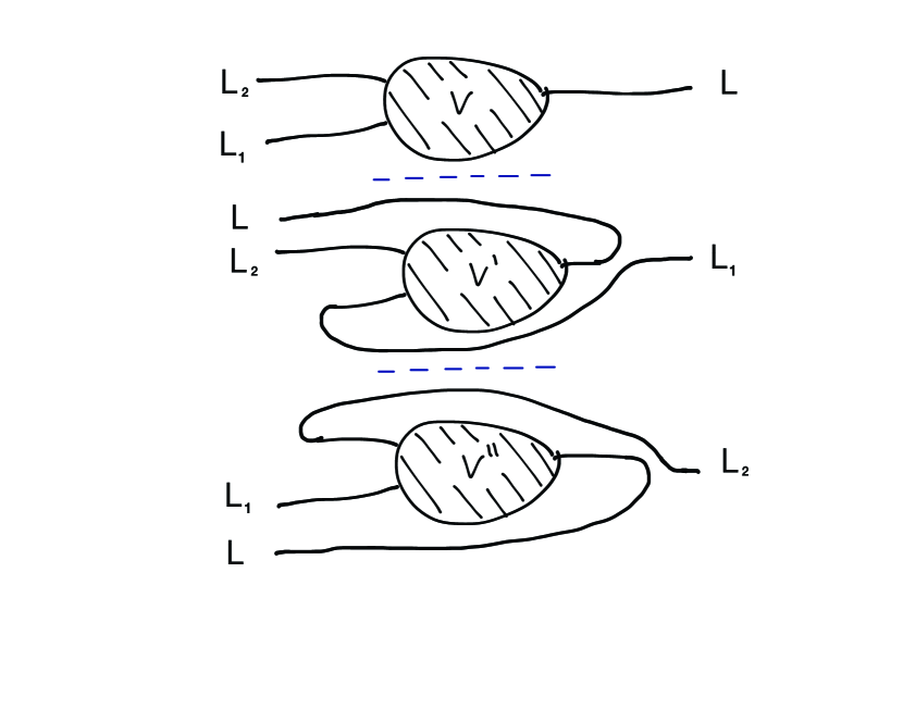
Figure 3. The cobordisms $V$ and $V^{\prime}$, $V^{\prime\prime}$ obtained by bending the ends of $V$ as indicated.

The proof of Corollary 1.1.2 is given in §4.8.3.

1.1.2. Floer homology and the bottom triangle in (1)

Let $N$ be an object in $D\mathcal{F}uk(M)$. There is an obvious functor

$$h_{N}:D\mathcal{F}uk(M)\xrightarrow{\hom(N,-)}(\mathcal{V},\times)$$

with values in the monoidal category $(\mathcal{V},\times)$ of ungraded vector spaces over $\mathbb{Z}_{2}$, with the monoidal structure $\times$ being direct product. (We thus ignore all the issues related to grading and orientations.) The functor $\mathcal{H}F_{N}$ in the diagram is the composition $\mathcal{H}F_{N}=h_{N}\circ\mathcal{F}$. Assuming now that $N\in\mathcal{L}$, we remark that the functor $\mathcal{H}F_{N}$ associates to each object $L$ in $S\mathcal{C}ob(M)$ the Floer homology $HF(N,L)$. Thus the functor $\mathcal{H}F_{N}$ encodes Floer homology as a sort of “Lagrangian Quantum Field Theory”: it is a vector space valued functor defined on a cobordism category that associates to each Lagrangian $L\in\mathcal{L}$ the Floer homology $\mathcal{H}F_{N}(L)=HF(N,L)$ (one could also complete $S\mathcal{C}ob(M)$ to a monoidal category over which $\mathcal{H}F_{N}$ extends monoidally thus bringing the formal properties of $\mathcal{H}F_{N}$ even closer to the axioms of a TQFT).

From this perspective the existence of Diagram 1 can be seen as a statement concerning the properties of the Floer homology functor. In particular, the existence of $\mathcal{F}$ reflects the naturality properties of $\mathcal{H}F_{N}$ with respect to $N$. Further properties involve the triangulated structure of $D\mathcal{F}uk(M)$ and they translate into the existence of the lift $\widetilde{\mathcal{F}}$.

In more concrete terms, as a consequence of Diagram (2), of Remark 1.1.1 and Theorem A, we immediately see that:

Corollary 1.1.3.

For any $N\in\mathcal{L}$ the Floer homology functor

$$\mathcal{H}F_{N}:S\mathcal{C}ob(M)\to(\mathcal{V},\times)$$

defined above has the following three properties:

• $\mathcal{H}F_{N}$ restricts to the Seidel representation on those cobordisms $V$ that are given as the Lagrangian suspension associated to a Hamiltonian isotopy acting on a given Lagrangian submanifold of $M$.

• If $V$ has just two negative ends $L_{1}$, $L_{2}$ and $V^{\prime}$, $V^{\prime\prime}$ are as in Corollary 1.1.2, then there is a long exact sequence that only depends on the horizontal isotopy type of $V$

  $$\ldots\longrightarrow\mathcal{H}F_{N}(L_{2})\xrightarrow{\mathcal{H}F_{N}(V^{\prime\prime})}\mathcal{H}F_{N}(L_{1})\xrightarrow{\mathcal{H}F_{N}(V^{\prime})}\mathcal{H}F_{N}(L)\xrightarrow{\mathcal{H}F_{N}(V)}\mathcal{H}F_{N}(L_{2})\longrightarrow\ldots$$

  and this long exact sequence is natural in $N$.

• More generally, if $V$ has negative ends $L_{1},L_{2},\ldots,L_{k}$ with $k\geq 2$, then there exists a spectral sequence $\mathcal{E}_{N}(V)=\{E^{r}_{p},d^{r}:E^{r}_{p}\longrightarrow E^{r}_{p-1}\}_{r\geq 0,p\in\mathbb{Z}}$, each page of which is graded by a single index, with $E^{r}_{p}=0$ for $p\leq 0$, and so that:

  • the first page of the spectral sequence satisfies: $E^{1}_{p}=HF(N,L_{p})$ for every $p\geq 1$. Moreover, the differential $d^{1}:E^{1}_{p}\longrightarrow E^{1}_{p-1}$ is given by $d^{1}=H(\pi_{p-1})\circ H(\psi_{p})$, where $H(\psi_{p})$ and $H(\pi_{p-1})$ are the Floer homological maps induced by the morphisms $\psi_{p}$ and $\pi_{p-1}$ from the exact triangles in Theorem A for $i=p-1,p$

    $$L_{p-1}[1]\xrightarrow{\,\psi_{p-1}\,} Z_{p-2}\longrightarrow Z_{p-1}\xrightarrow{\,\pi_{p-1}\,}L_{p-1},$$

    $$L_{p}[1]\xrightarrow{\,\psi_{p}\,} Z_{p-1}\longrightarrow Z_{p}\xrightarrow{\,\pi_{p}\,}L_{p}.$$

  • from the first page on, the terms of the spectral sequence only depend on $N$ and the horizontal isotopy type of $V$. Furthermore, the sequence is natural in $N$.

  • $\mathcal{E}_{N}(V)$ collapses at page $r=k$ and converges to $\mathcal{H}F_{N}(L)$.

1.2. Relation to $K$-theory

The cobordism category $\mathcal{C}ob$ of a symplectic manifold $M$ gives rise to a group $G_{cob}(M)$ somewhat analogous to cobordism groups in differential topology. For this end we first consider the free abelian group $F_{\mathcal{L}}$ generated by the Lagrangian submanifolds $L\in\mathcal{L}$. We then define a subgroup of relations $R_{\mathcal{L}}\subset F_{\mathcal{L}}$ as the subgroup generated by all elements of the form $L_{1}+\cdots+L_{r}$ for which there exists a Lagrangian cobordism $V\in\mathcal{L}_{cob}$ without any positive end and whose negative ends consist of $(L_{1},\ldots,L_{r})$ (i.e. $(L_{1},\ldots,L_{r})$ is null Lagrangian cobordant). We define $G_{cob}(M)=F_{\mathcal{L}}/R_{\mathcal{L}}$.

One can alter the above and make other meaningful definitions. For example, one can consider also a non-abelian version of $G_{cob}$ in which the order of the Lagrangians $(L_{1},\ldots,L_{r})$ on the positive end plays a role (see e.g. [BC2]). Another possible variation is to consider the Lagrangians $L\in\mathcal{L}$ together with additional structures such as orientations, spin structures, grading, local systems etc. One defines then the relations as above by requiring in addition that these structures extend over the cobordism $V$.

Next consider the $K$-theory group (or Grothendieck group) $K_{0}(D\mathcal{F}uk(M))$ of the derived Fukaya category of $M$. Recall that this group is the abelian group generated by the objects of $D\mathcal{F}uk(M)$ modulo the following collection of relations: every exact triangle

$$X\longrightarrow Y\longrightarrow Z\longrightarrow X[-1]$$

contributes the relation $X-Y+Z=0$. (In our case the Fukaya category is not graded, hence $Y=-Y$ for every object $Y$.)

Corollary 1.2.1.

The mapping $\mathcal{L}\longrightarrow K_{0}(D\mathcal{F}uk(M))$ given by $L\longmapsto L$ induces a well defined homomorphism of groups

(3) $$\Theta:G_{cob}(M)\longrightarrow K_{0}(D\mathcal{F}uk(M)).$$

The proof follows immediately from Theorem A. Indeed, let $L_{1}+\cdots+L_{r}$ be a generator of $R_{\mathcal{L}}$, so that we have a Lagrangians cobordism $V$ without positive ends and with negative ends $(L_{1},\ldots,L_{r})$. By Theorem A we have objects $Z_{1}\simeq L_{1}$, $Z_{2},\ldots,Z_{r-1}$, $Z_{r}\simeq 0$ in $D\mathcal{F}uk(M)$ and a sequence of exact triangles:

$$L_{i}[1]\longrightarrow Z_{i-1}\longrightarrow Z_{i}\longrightarrow L_{i},\quad\forall\;2\leq i\leq r.$$

From this we obtain the following identities in $K_{0}(D\mathcal{F}uk(M))$:

$$Z_{1}=L_{1},\quad Z_{i}=L_{i}+Z_{i-1}\;\;\forall\;2\leq i\leq r,\quad Z_{r}=0.$$

Summing these identities up, it readily follows that $L_{1}+\cdots+L_{r}=0$ in $K_{0}(D\mathcal{F}uk(M))$. This proves that $R_{\mathcal{L}}$ is sent to $0\in K_{0}(D\mathcal{F}uk(M))$ under the mapping $F_{\mathcal{L}}\longrightarrow K_{0}(D\mathcal{F}uk(M))$, induced by $L\longmapsto L$, hence the homomorphism $\Theta$ is well defined.

An interesting question is when is the homomorphism $\Theta$ an isomorphism. This question can sometimes be studied with the help of homological mirror symmetry at least in those cases where it has been established. More precisely, if there exists a triangulated equivalence between an appropriate completion $D^{c}\mathcal{F}uk(M)$ of $D\mathcal{F}uk(M)$ and the bounded derived category of coherent sheaves $D^{b}Coh(M^{\vee})$ on the mirror manifold $M^{\vee}$, then there is an isomorphism between the associated $K$-groups: $K_{0}(D^{c}\mathcal{F}uk(M))\cong K(M^{\vee})$. The point is that in some cases the latter group is well known. One can then combine such algebro-geometric information together with constructions of Lagrangian cobordisms on the “$M$”-side, e.g. surgery (see §6 in [BC2]), in order to study the homomorphism $\Theta$.

For such an approach one needs sometimes to adjust a bit the definitions of $\mathcal{C}ob$ and $D\mathcal{F}uk(M)$ to include more structures, as indicated above, or to work with particular classes of Lagrangian submanifolds $\mathcal{L}$. The simplest non-trivial example seems to be $M=\mathbb{T}^{2}$ (and $M^{\vee}=$ elliptic curve). Recent results of Haug [Hau1, Hau2] show that in this case an appropriate version of $\Theta$ (defined for a suitable class $\mathcal{L}$) is indeed an isomorphism.

1.3. Outline of the proof of Theorem B

The proof has essentially two main steps.

1.3.1. The Fukaya category of cobordisms

As mentioned before, the first step is to define a Fukaya category of cobordisms in $\mathbb{R}^{2}\times M$, which we denote $\mathcal{F}uk_{cob}(\mathbb{R}^{2}\times M)$. The construction follows the set-up in Seidel’s book [Sei3]. In particular, the regularity of the relevant moduli spaces is insured by perturbing the Cauchy-Riemann equation by Hamiltonian terms. Compared to the construction in [Sei3], there are two additional major issues that have to be addressed in our setting: the first is that we work in a monotone situation and no longer an exact one. The second is that Lagrangian cobordisms are embedded in a non-compact ambient manifold, $\mathbb{R}^{2}\times M$, and the total spaces of these cobordisms are non compact Lagrangians. Thus we need to deal with compactness issues as well as with regularity at $\infty$. Adapting the construction from the exact setting to the monotone one is in fact non-problematic: it uses the same type of arguments as in our previous work [BC1]. The non-compactness issue turns out to be considerably more delicate. As in [BC2], the main tool that we use to insure the compactness of moduli spaces of perturbed $J$-holomorphic curves $\mathbf{u}$ is based on the open mapping theorem for holomorphic functions in the plane. There is however a difficulty in implementing this strategy directly. On one hand, the Hamiltonian perturbations needed to construct the $A_{\infty}$-category have to be picked in such a way as to insure regularity, including at infinity, which requires perturbations that are not compactly supported. On the other hand, to apply the compactness argument based on the open mapping theorem we need that, outside of a compact in $\mathbb{R}^{2}\times M$, the curves ${\bf u}$ satisfy a horizontally homogeneous equation in the sense that the projections to $\mathbb{R}^{2}\cong\mathbb{C}$ of the curves ${\bf u}$ are holomorphic. These two constraints: perturbations that are non-trivial at $\infty$ and horizontally homogeneous equations are in general incompatible! To deal with this point we define the relevant moduli spaces using curves ${\bf u}$ that satisfy perturbed $J$-holomorphic equations with Hamiltonian perturbation terms that do not vanish at $\infty$ but that have a special behavior away from a fixed, sufficiently big compact. The Hamiltonian perturbations are so that the curves ${\bf u}$ transform by a specific change of variable - also known as a naturality transformation - to curves ${\bf v}$ that are horizontally homogeneous at infinity. Compactness for the curves ${\bf v}$ implies then the desired compactness for the curves ${\bf u}$. The naturality transformation can be implemented in a coherent way along all the moduli spaces used to define the $A_{\infty}$-multiplications (see §3.1) but then two further problems arise. First, the boundary conditions for the curves ${\bf u}$ are slightly different from those considered e.g. in [Sei3] and thus energy bounds have to be verified explicitly as they do not directly result from the calculations in [Sei3]. A second and more serious issue is that the boundary conditions for the curves ${\bf v}$ are not fixed but rather moving ones. As a consequence, proving compactness for the curves ${\bf v}$ is not quite immediate and requires additional precision in the choice of perturbations. This is implemented in §3.1 and §3.3, where we use the term bottleneck to indicate the particular profile of the Hamiltonians that are adapted to this purpose. (See e.g. Figure 8 in §3.2.) These choices of particular Hamiltonian perturbations come back with a vengeance and complicate to a large extent the proofs of various properties of the resulting $A_{\infty}$-category such as invariance.

1.3.2. Inclusion, triangles and $\widetilde{\mathcal{F}}$

To construct the functor $\widetilde{\mathcal{F}}$ we first compare the two categories $\mathcal{F}uk(M)$, $\mathcal{F}uk_{cob}(\mathbb{R}^{2}\times M)$. Namely, we show that if $\gamma:\mathbb{R}\to\mathbb{R}^{2}$ is a curve in the plane with horizontal ends, then there is an induced functor of $A_{\infty}$-categories:

$$\mathcal{I}_{\gamma}:\mathcal{F}uk(M)\to\mathcal{F}uk_{cob}(\mathbb{R}^{2}\times M)$$

defined on the corresponding Fukaya category of $M$. On objects this functor is defined by $\mathcal{I}_{\gamma}(L)=\gamma\times L$.

Denote $\mathcal{A}=\mathcal{F}uk(M)$ and $\widetilde{\mathcal{A}}=\mathcal{F}uk_{cob}(\mathbb{R}^{2}\times M)$. There is a Yoneda embedding functor

$$\mathcal{Y}:\mathcal{A}\to\textnormal{\sl fun}(\mathcal{A},Ch^{opp}),$$

where the right-hand side stands for $A_{\infty}$-functors from $\mathcal{A}$ to the opposite category of chain complexes viewed as a dg-category. A similar Yoneda embedding is defined also on $\widetilde{\mathcal{A}}$.

Fix now a cobordism $(V;L_{1}\cup\ldots\cup L_{k},L)$ as in Figure 4. Given any curve $\gamma$ as above, there is a functor $\mathcal{M}_{V,\gamma}:\mathcal{A}\to Ch^{opp}$ defined by

$$\mathcal{M}_{V,\gamma}=\mathcal{Y}(V)\circ\mathcal{I}_{\gamma}~{}.~{}$$

At the derived level, this functor only depends on the horizontal isotopy classes of $V$ and $\gamma$. We consider a particular set of curves $\alpha_{1},\ldots,\alpha_{k}\subset\mathbb{R}^{2}$ basically as in Figure 4. Therefore, we get a sequence of functors $\mathcal{M}_{V,i}:=\mathcal{M}_{V,\alpha_{i}}$, $i=1,\ldots,k$.

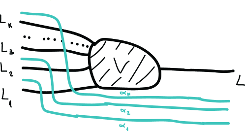
Figure 4. A cobordism $V$ together with curves of the type $\alpha_{i}$’s.

We then show that these functors are related by exact triangles (in the sense of triangulated $A_{\infty}$ categories):

(4) $$T^{-1}\mathcal{Y}(L_{s})\to\mathcal{M}_{V,s-1}\to\mathcal{M}_{V,s}\to\mathcal{Y}(L_{s})\;\;\forall\ 2\leq s\leq k.$$

Moreover, there is a quasi-isomorphism $\phi_{V}:\mathcal{Y}(L)\to\mathcal{M}_{V,k}$. The proof of this fact requires the same type of arguments that appeared earlier in constructing the Fukaya cobordism category together with some new geometric ingredients. In particular, the key ingredient to show the existence of the exact triangles (4) is the fact that, with appropriate choices of data, the relevant perturbed holomorphic curves $\mathbf{u}$ that contribute to the $A_{\infty}$ operations transform by naturality into curves $\mathbf{v}$ whose projection is holomorphic around the intersections of the curves $\alpha_{i}$ and the projection of $V$. By taking into account orientations and using again the open mapping theorem it then follows that if such a curve (viewed as punctured polygon) has as entries intersection points involving some of the first $s$ ends of $V$, then it has as exit an intersection point also involving one of these ends. The exact sequences (4) are an algebraic translation of this fact.

With the exact sequences (4) established, the definition of $\widetilde{\mathcal{F}}$ is relatively direct, by translating the preceding structure to the derived setting. Finally, we verify that $\widetilde{\mathcal{F}}$ respects composition which is again a non-trivial step.

Remark 1.3.1.

a. Apriori, a different approach to the construction of the Fukaya category of cobordisms, that avoids the difficult perturbation issues above, would be to use for the definition of all the relevant moduli spaces only horizontally homogeneous equations. In this case, compactness is automatic but the algebraic output of the construction is not an $A_{\infty}$-category but a weaker structure sometimes called a pre-$A_{\infty}$-category. For instance, the Floer complex $CF(V,V^{\prime})$ for two cobordisms $V$ and $V^{\prime}$ is only defined if $V$ and $V^{\prime}$ are distinct at $\infty$. This leads to a plethora of further complications. It is not clear whether this other approach can lead to a proof of Theorem B and, even more, to one shorter than the proof here.

b. As explained in §1.3.2, transforming the curves $\mathbf{u}$ by naturality to curves $\mathbf{v}$ whose projection is holomorphic outside of a certain compact $\subset\mathbb{C}$ is important for the proof of Theorem B not only to define the Fukaya category of cobordisms but also in the second step, where specific properties of planar holomorphic curves enter the argument. Indeed, we actually need at that point rather fine control on the region of holomorphicity of the projection of $\mathbf{v}$ in the sense that it is not sufficient for holomorphicity to take place at infinity but also in regions where various cylindrical projections of the Lagrangians involved intersect.

Fukaya categories in a variety of other non-compact situations have appeared before in the literature, in particular in [AS] and in [Sei4]. The construction in Seidel’s paper [Sei4] is closest to the construction here and a number of results from that paper are used here. Moreover, a rather straightforward adaptation of the methods in [Sei4] leads to a category with objects cobordisms with ends only on one side (that is cobordisms of the type $V:\emptyset\to(L_{1},\ldots,L_{k})$). Compactness, is insured in [Sei4] by a variant of the maximum principle for harmonic functions and, while it does require a special form of “disjoining” planar hamiltonian perturbations, all naturality issues are bypassed. However, this setup is not applicable, at least directly, to the proof of Theorem B not only because we need to deal with cobordisms with arbitrary ends but, more importantly, because implementing the second step of the proof in this setup does not seem immediate. In short, our choice here is to construct the category $\mathcal{F}uk_{cob}(\mathbb{C}\times M)$ in a form that is directly applicable to the proof of Theorem B. The construction in itself provides an alternative approach to that in [Sei4] and is potentially of some independent interest.

Acknowledgments

Part of this work was accomplished during a stay at the Institute for Advanced Study in Princeton. We thank Helmut Hofer and the IAS for their gracious hospitality. We would also like to thank the referee for a very careful reading of the paper and for making many comments helping to improve the quality of the exposition.

2. Prerequisites

Here we fix the setting of the paper, in particular the definition of the Lagrangian cobordism category that we use, the relevant Fukaya category as well as all the auxiliary constructions and conventions needed in the paper. Note that from now on and through the remainder of the paper, a part of the notation from the Introduction will change. Namely, the class of Lagrangian submanifolds $\mathcal{L}$ will be denoted $\mathcal{L}^{*}_{d}$, the class of admissible cobordisms by $\mathcal{L}_{d}(\mathbb{C}\times M)$, the category $\mathcal{C}ob$ will be denoted by $\mathcal{C}ob^{d}_{0}$ and $\mathcal{F}uk$ by $\mathcal{F}uk^{d}$. The meaning of the decorations $d$, $*$ and $0$ in this notation will be explained below.

We assume here that the manifold $(M^{2n},\omega)$ is compact. Lagrangian submanifolds $L\subset M$ will be generally assumed to be closed unless otherwise indicated.

The subsections §2.1, §2.2, §2.3 and §2.4 are just recalls of various definitions and constructions from [BC2] and §2.5 concerns the Fukaya category. Subsection 2.6 contains a description of the $T^{S}(-)$ construction that is more detailed and precise than the one in [BC2].

2.1. Monotonicity

All families of Lagrangian submanifolds in our constructions have to satisfy a monotonicity condition in a uniform way as described below. Given a Lagrangian submanifold $L\subset M$ let

$$\omega:\pi_{2}(M,L)\to\mathbb{R}\ ,\ \mu:\pi_{2}(M,L)\to\mathbb{Z}$$

be the morphism given, respectively, by integration of $\omega$ and by the Maslov index. The Lagrangian $L$ is monotone if there exists a positive constant $\rho>0$ so that for all $\alpha\in\pi_{2}(M,L)$ we have $\omega(\alpha)=\rho\mu(\alpha)$ and moreover the minimal Maslov number

$$N_{L}:=\min\{\mu(\alpha):\alpha\in\pi_{2}(M,L)\ ,\ \omega(\alpha)>0\}$$

satisfies $N_{L}\geq 2$.

We will use $K=\mathbb{Z}_{2}$ as the ground ring. However, we mention here that most of the discussion generalizes to arbitrary rings under additional assumptions on the Lagrangians.

For a closed, monotone Lagrangian $L$ there is an associated basic Gromov-Witten type invariant $d_{L}\in\mathbb{Z}_{2}$ given as the number (mod $2$) of $J$-holomorphic disks of Maslov index $2$ going through a generic point $P\in L$ for $J$ a generic almost complex structure that is compatible with $\omega$.

A family of Lagrangian submanifolds $L_{i}$, $i\in I$, is uniformly monotone if each $L_{i}$ is monotone and the following condition is satisfied: there exists $d\in K$ so that for all $i\in I$ we have $d_{L_{i}}=d$ and there exists a positive real constant $\rho$ so that the monotonicity constant of $L_{i}$ equals $\rho$ for all $i\in I$. All the Lagrangians used in the paper will be assumed monotone and, similarly, the Lagrangian families will be assumed uniformly monotone.

For $d\in\mathbb{Z}_{2}$ and $\rho\geq 0$, we let $\mathcal{L}_{d}(M)$ be the family of closed, connected Lagrangian submanifolds $L\subset M$ that are monotone with monotonicity constant $\rho$ and with $d_{L}=d$ (we thus suppress $\rho$ from the notation).

2.2. Cobordism: main definitions

The plane $\mathbb{R}^{2}$ is endowed with the symplectic structure $\omega_{\mathbb{R}^{2}}=dx\wedge dy$, $(x,y)\in\mathbb{R}^{2}$. The product $\widetilde{M}=\mathbb{R}^{2}\times M$ is endowed with the symplectic form $\omega_{\mathbb{R}^{2}}\oplus\omega$. We denote by $\pi:\mathbb{R}^{2}\times M\to\mathbb{R}^{2}$ the projection. For a subset $V\subset\mathbb{R}^{2}\times M$ and $S\subset\mathbb{R}^{2}$ we let $V|_{S}=V\cap\pi^{-1}(S)$.

Definition 2.2.1.

Let $(L_{i})_{1\leq i\leq k_{-}}$ and $(L^{\prime}_{j})_{1\leq j\leq k_{+}}$ be two families of closed Lagrangian submanifolds of $M$. We say that that these two (ordered) families are Lagrangian cobordant, $(L_{i})\simeq(L^{\prime}_{j})$, if there exists a smooth compact cobordism $(V;\coprod_{i}L_{i},\coprod_{j}L^{\prime}_{j})$ and a Lagrangian embedding $V\subset([0,1]\times\mathbb{R})\times M$ so that for some $\epsilon>0$ we have:

(5) $$V|_{[0,\epsilon)\times\mathbb{R}}= \coprod_{i}([0,\epsilon)\times\{i\})\times L_{i}$$

$$V|_{(1-\epsilon,1]\times\mathbb{R}}= \coprod_{j}((1-\epsilon,1]\times\{j\})\times L^{\prime}_{j}~{}.~{}$$

The manifold $V$ is called a Lagrangian cobordism from the Lagrangian family $(L^{\prime}_{j})$ to the family $(L_{i})$. We denote such a cobordism by $V:(L^{\prime}_{j})\leadsto(L_{i})$ or $(V;(L_{i}),(L^{\prime}_{j}))$.

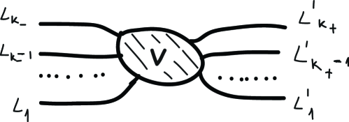
Figure 5. A cobordism $V:(L^{\prime}_{j})\leadsto(L_{i})$ projected on $\mathbb{R}^{2}$.

A cobordism is called monotone if

$$V\subset([0,1]\times\mathbb{R})\times M$$

is a monotone Lagrangian submanifold.

It is often more convenient to view cobordisms as embedded in $\mathbb{R}^{2}\times M$. Given a cobordism $V\subset([0,1]\times\mathbb{R})\times M$ as in Definition 2.2.1 we can extend trivially its negative ends towards $-\infty$ and its positive ends to $+\infty$ thus getting a Lagrangian $\overline{V}\subset\mathbb{R}^{2}\times M$. We will in general not distinguish between $V$ and $\overline{V}$ but if this distinction is needed we will call

(6) $$\overline{V}=\Bigl{(}\coprod_{i}(-\infty,0]\times\{i\}\times L_{i}\Bigr{)}\cup V\cup\Bigl{(}\coprod_{j}[1,\infty)\times\{j\}\times L^{\prime}_{j}\Bigr{)}$$

The $\mathbb{R}$-extension of $V$. At certain points in the paper we will also use Lagrangians in $\mathbb{R}^{2}\times M$ that are $\mathbb{R}$-extensions of cobordisms $V\subset([a,b]\times\mathbb{R})\times M$. The definition of such cobordims is identical with the one above except with the interval $[a,b]$ replacing $[0,1]$.

More generally, by a Lagrangian submanifold with cylindrical ends we mean a Lagrangian submanifold $\overline{V}\subset\widetilde{M}$ without boundary that has the following properties:

1. For every $a<b$ the subset $\overline{V}|_{[a,b]\times\mathbb{R}}$ is compact.

2. There exists $R_{+}$ such that

   $$\overline{V}|_{[R_{+},\infty)\times\mathbb{R}}=\coprod_{i=1}^{k_{+}}[R_{+},\infty)\times\{a^{+}_{i}\}\times L^{+}_{i}$$

   for some $a^{+}_{1}<\cdots<a^{+}_{k_{+}}$ and some Lagrangian submanifolds $L^{+}_{1},\ldots,L^{+}_{k_{+}}\subset M$.

3. There exists $R_{-}\leq R_{+}$ such that

   $$\overline{V}|_{(-\infty,R_{-}]\times\mathbb{R}}=\coprod_{i=1}^{k_{-}}(-\infty,R_{-}]\times\{a^{-}_{i}\}\times L^{-}_{i}$$

   for some $a^{-}_{1}<\cdots<a^{-}_{k_{-}}$ and some Lagrangian submanifolds $L^{-}_{1},\ldots,L^{-}_{k_{-}}\subset M$.

We allow $k_{+}$ or $k_{-}$ to be $0$ in which case $\overline{V}|_{[R_{+},\infty)\times\mathbb{R}}$ or $\overline{V}|_{(-\infty,R_{-}]\times\mathbb{R}}$ are void.

For every $R\geq R_{+}$ write $E^{+}_{R}(\overline{V})=\overline{V}|_{[R,\infty)\times\mathbb{R}}$ and call it a positive cylindrical end of $\overline{V}$. Similarly, we have for $R\leq R_{-}$ a negative cylindrical end $E^{-}_{R}(\overline{V})$.

If $\overline{W}$ is a Lagrangian submanifold with cylindrical ends then by an obvious modification of the ends (and a possible symplectomorphism on the $\mathbb{R}^{2}$ component) it is easy to obtain a Lagrangian cobordism between the families of Lagrangians corresponding to the positive and negative ends of $\overline{W}$.

In order to simplify terminology, we will say that a Lagrangian with cylindrical ends $\overline{V}$ is cylindrical outside of a compact subset $K\subset\mathbb{R}^{2}$ if $\overline{V}|_{\mathbb{R}^{2}\setminus K}$ consists of horizontal ends, i.e. it is of the form $E^{-}_{R_{-}}(\overline{V})\cup E^{+}_{R_{+}}(\overline{V})$.

We will also need the following notion.

Definition 2.2.2.

Two Lagrangians with cylindrical ends $\overline{V},\overline{W}\subset\widetilde{M}$ are said to be cylindrically distinct at infinity if there exists $R>0$ such that $\pi(E^{+}_{R}(\overline{V}))\cap\pi(E^{+}_{R}(\overline{W}))=\emptyset$ and $\pi(E^{-}_{-R}(\overline{V}))\cap\pi(E^{-}_{-R}(\overline{W}))=\emptyset$.

Finally, here is a class of Hamiltonian isotopies that will be useful in the following.

Definition 2.2.3 (Horizontal isotopies).

Let $\{\overline{V_{t}}\}_{t\in[0,1]}$ be an isotopy of Lagrangian submanifolds of $\widetilde{M}$ with cylindrical ends. We call this isotopy horizontal if there exists a (not necessarily compactly supported) Hamiltonian isotopy $\{\psi_{t}\}_{t\in[0,1]}$ of $\widetilde{M}$ with $\psi_{0}={{\mathchoice{\rm 1\mskip-4.0mul}{\rm 1\mskip-4.0mul}{\rm 1\mskip-4.5mul}{\rm 1\mskip-5.0mul}}}$ and with the following properties:

1. $\overline{V_{t}}=\psi_{t}(\overline{V_{0}})$ for all $t\in[0,1]$.

2. There exist real numbers $R^{\prime}_{-}<R_{-}<R_{+}<R^{\prime}_{+}$ such that for all $t\in[0,1]$, $x\in E^{\pm}_{R^{\prime}_{\pm}}(\overline{V_{0}})$ we have $\psi_{t}(x)\in E^{\pm}_{R_{\pm}}(\overline{V_{0}})$.

3. There is a constant $K>0$ so that for all $x\in E^{\pm}_{R_{\pm}}(\overline{V_{0}})$, $|d\pi_{x}(X_{t}(x))|<K$. Here $X_{t}$ is the (time dependent) vector field of the flow $\{\psi_{t}\}_{t\in[0,1]}$.

We say that two Lagrangians $\overline{V},\overline{V^{\prime}}\subset\widetilde{M}$ with cylindrical ends are horizontally isotopic if there exists an isotopy as above $\{\overline{V_{t}}\}_{t\in[0,1]}$ with $\overline{V_{0}}=\overline{V}$ and $\overline{V_{1}}=\overline{V^{\prime}}$. We will sometimes say that an ambient Hamiltonian isotopy $\{\psi_{t}\}_{t\in[0,1]}$ as above is horizontal with respect to $\overline{V_{0}}$.

2.3. The category $\mathcal{C}ob^{d}_{0}(M)$

Consider first the following category $\widetilde{{\mathcal{C}ob}^{d}}(M)$, $d\in K$. Its objects are families $(L_{1},L_{2},\ldots,L_{r})$ with $r\geq 1$, $L_{i}\in\mathcal{L}_{d}(M)$. (Recall that $\mathcal{L}_{d}(M)$ stands for the class of uniformly monotone Lagrangians $L$ with $d_{L}=d$ with the same monotonicity constant $\rho$ which is omitted from the notation.) We will denote by $\mathcal{L}_{d}(\mathbb{C}\times M)$ the Lagrangians in $\mathbb{C}\times M$ that satisfy the same conditions: they are uniformly monotone with the same $d_{V}=d$ and the same monotonicity constant $\rho$.

To describe the morphisms in this category we proceed in two steps. First, for any two horizontal isotopy classes of cobordisms $[V]$ and $[U]$ with $V:(L^{\prime}_{j})\leadsto(L_{i})$ (as in Definition 2.2.1) and $U:(K^{\prime}_{s})\leadsto(K_{r})$ we define the sum $[V]+[U]$ to be the horizontal isotopy class of a cobordism $W:(L^{\prime}_{j})+(K^{\prime}_{s})\leadsto(L_{i})+(K_{r})$ so that $W=V\coprod\widetilde{U}$ with $\widetilde{U}$ a suitable translation up the $y$-axis of a cobordism horizontally isotopic to $U$ so that $\widetilde{U}$ is disjoint from $V$.

The morphisms in $\widetilde{{\mathcal{C}ob}^{d}}(M)$ are now defined as follows. A morphism

$$[V]\in{\textnormal{Mor\/}}\bigl{(}(L^{\prime}_{j})_{1\leq j\leq S},(L_{i})_{1\leq i\leq T}\bigr{)}$$

is a horizontal isotopy class that is written as a sum $[V]=[V_{1}]+\cdots+[V_{S}]$ with each $V_{j}\in\mathcal{L}_{d}(\mathbb{C}\times M)$ a cobordism from the Lagrangian family formed by the single Lagrangian $L^{\prime}_{j}$ and a subfamily $(L_{r(j)},\ldots,L_{r(j)+s(j)})$ of the $(L_{i})$’s, and so that $r(j)+s(j)+1=r(j+1)$. In other words, $V$ decomposes as a union of $V_{i}$’s each with a single positive end but with possibly many negative ones. We will often denote such a morphism by $V:(L^{\prime}_{j})\longrightarrow(L_{i})$.

The composition of morphisms is induced by concatenation followed by a rescaling to reduce the “width” of the cobordism to the interval $[0,1]$.

We consider here the void set as a Lagrangian of arbitrary dimension. We now intend to factor both the objects and the morphisms in this category by equivalence relations that will transform this category in a strict monoidal one. For the objects the equivalence relation is induced by the relations

(7) $$(L,\emptyset)\sim(\emptyset,L)\sim(L).$$

At the level of the morphisms a bit more care is needed. For each $L\in\mathcal{L}_{d}(M)$ we will define two particular cobordisms $\Phi_{L}:(\emptyset,L)\leadsto(L,\emptyset)$ and $\Psi_{L}:(L,\emptyset)\leadsto(\emptyset,L)$ as follows. Let $\gamma:[0,1]\to[0,1]$ be an increasing, surjective smooth function, strictly increasing on $(\epsilon,1-\epsilon)$ and with $\gamma^{\prime}(t)=0$ for $t\in[0,\epsilon]\cup[1-\epsilon,1]$. We now let $\Phi(L)=graph(\gamma)\times L$ and $\Psi(L)=graph(1-\gamma)\times L$. The equivalence relation for morphisms is now induced by the following two identifications:

1. For every cobordism $V$ we identify $V+\emptyset\sim\emptyset+V\sim V$, where $\emptyset$ is the void cobordism between two void Lagrangians.

2. If $V:L\longrightarrow(L_{1},...,L_{i},\emptyset,L_{i+2},\ldots,L_{k})$, then we identify $V\sim V^{\prime}\sim V^{\prime\prime}$, where $V^{\prime}=\Phi_{L_{i+2}}\circ V$, $V^{\prime\prime}=\Psi_{L_{i}}\circ V.$

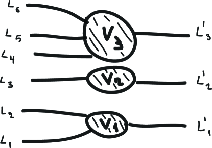
Figure 6. A morphism $V:(L^{\prime}_{1},L^{\prime}_{2},L^{\prime}_{3})\longrightarrow(L_{1},\ldots,L_{6})$, $V=V_{1}+V_{2}+V_{3}$, projected to $\mathbb{R}^{2}$.

To construct the category $\mathcal{C}ob^{d}(M)$ we now consider the full subcategory $\mathcal{S}\subset\widetilde{\mathcal{C}ob}^{d}(M)$ obtained by restricting the objects only to those families $(L_{1},\ldots,L_{k})$ with $L_{i}$ non-narrow for all $1\leq i\leq k$. Recall that a monotone Lagrangian is non-narrow if its quantum homology $QH(L)$ (with $\Lambda=\mathbb{Z}_{2}[t,t^{-1}]$ coefficients) does not vanish. Then $\mathcal{C}ob^{d}(M)$ is obtained by the quotient of the objects of $\mathcal{S}$ by the equivalence relation in (7) and the quotient of the morphisms of $\mathcal{S}$ by the equivalence relation in (Eq 1), (Eq 2).

This category is called the Lagrangian cobordism category of $M$. As mentioned before, it is a strict monoidal category, where the monoidal structure is defined on objects by concatenating tuples of Lagrangians and on morphisms by taking disjoint unions of cobordisms, possibly after a suitable Hamiltonian isotopy.

The Theorem B requires an additional assumption on all the Lagrangians in our constructions. Every Lagrangian $L$ is required to satisfy:

(8) $$\pi_{1}(L)\stackrel{{\scriptstyle i_{\ast}}}{{\longrightarrow}}\pi_{1}(M)\ \ \ \mathrm{vanishes},$$

where $i_{\ast}$ is induced by the inclusion $L\subset M$. Alternatively, in case the first Chern class $c_{1}$ and $\omega$ are proportional as morphisms defined on $H_{2}(M;\mathbb{Z})$ (and not only on $\pi_{2}(M)$) it is enough to assume that the image of $i_{\ast}$ is torsion. An analogous constraint is imposed also to the Lagrangian cobordisms involved.

We denote by $\mathcal{L}^{\ast}_{d}(M)$ the Lagrangians in $\mathcal{L}_{d}(M)$ that are non-narrow and additionally satisfy (8). There is a subcategory of $\mathcal{C}ob^{d}(M)$, that will be denoted by $\mathcal{C}ob^{d}_{0}(M)$, whose objects consist of families of Lagrangians each one belonging to $\mathcal{L}^{\ast}_{d}(M)$ and whose morphisms are represented by Lagrangian cobordisms $V$ satisfying the analogous condition to (8), but in $\mathbb{R}^{2}\times M$. This is again a strict monoidal category.

2.4. Floer homology

In this subsection we recall some basic notation and definitions concerning Lagrangian Floer homology. We refer the reader to [Oh1, Oh2, Oh3] for the foundations of Floer homology for monotone Lagrangians, and to [FOOO1, FOOO2] for the general case.

2.4.1. Lagrangian Floer homology

Let $L_{0},L_{1}\subset M$ be two monotone Lagrangian submanifolds with $d_{L_{0}}=d_{L_{1}}=d$. We assume in addition that $L_{0}$ and $L_{1}$ have the same monotonicity constant (or in other words that the pair $(L_{0},L_{1})$ is uniformly monotone).

We assume that condition (8) is satisfied by all the Lagrangians and cobordisms in the paper. An observation due to Oh [Oh1] shows that in this case one can construct Floer complexes and the associated homology with coefficients in $\mathbb{Z}_{2}$ as summarized below.

Denote by $\mathcal{P}(L_{0},L_{1})=\{\gamma\in C^{0}([0,1],M)\mid\gamma(0)\in L_{0},\gamma(1)\in L_{1}\}$ the space of paths in $M$ connecting $L_{0}$ to $L_{1}$. For $\eta\in\pi_{0}(\mathcal{P}(L_{0},L_{1}))$ we denote the path connected component of $\eta$ by $\mathcal{P}_{\eta}(L_{0},L_{1})$.

Fix $\eta\in\pi_{0}(\mathcal{P}(L_{0},L_{1}))$ and let $H:[0,1]\times M\to\mathbb{R}$ be a Hamiltonian function with Hamiltonian flow $\psi_{t}^{H}$. We assume that $\psi_{1}^{H}(L_{0})$ is transverse to $L_{1}$. Denote by $\mathcal{O}_{\eta}(H)$ the set of paths $\gamma\in\mathcal{P}_{\eta}(L_{0},L_{1})$ which are orbits of the flow $\psi^{H}_{t}$. Finally, we choose also a generic $1$-parametric family of almost complex structures $\mathbf{J}=\{J_{t}\}_{t\in[0,1]}$ compatible with $\omega$.

The Floer complex $CF(L_{0},L_{1};\eta;H,\mathbf{J})$ with coefficients in $\mathbb{Z}_{2}$ is generated as a $\mathbb{Z}_{2}$-vector space by the elements of $\mathcal{O}_{\eta}(H)$. The Floer differential

$$\partial:CF(L_{0},L_{1};\eta;H,\mathbf{J})\longrightarrow CF(L_{0},L_{1};\eta;H,\mathbf{J})$$

is defined as follows. For a generator $\gamma_{-}\in\mathcal{O}_{\eta}(H)$ we put

$$\partial(\gamma_{-})=\sum_{\scriptscriptstyle\gamma_{+}\in\mathcal{O}_{\eta}(H)}\#_{2}(\mathcal{M}_{0}(\gamma_{-},\gamma_{+};H,\mathbf{J}))\gamma_{+}.$$

Here $\mathcal{M}_{0}(\gamma_{-},\gamma_{+};H,\mathbf{J})$ stands for the $0$-dimensional components of the moduli space of finite energy strips $u:\mathbb{R}\times[0,1]\longrightarrow M$ connecting $\gamma_{-}$ to $\gamma_{+}$ that satisfy the Floer equation

(9) $$\partial_{s}u+J\partial_{t}u+\nabla H(t,u)=0$$

modulo the $\mathbb{R}$-action coming from translation in the $\mathbb{R}$ coordinate; the number of elements in $\mathcal{M}_{0}(\gamma_{-},\gamma_{+};H,\mathbf{J})$ is finite due to condition (8) and is counted over $\mathbb{Z}_{2}$.

Remark 2.4.1.

In this paper the Floer complexes, $CF(-)$, are defined over $\mathbb{Z}_{2}$ and are not graded. Hence the associated Floer homology $HF(-)$ is also un-graded. In special situations one can endow $CF(-)$ with some grading though not always over $\mathbb{Z}$ (e.g. when $L_{0}$ and $L_{1}$ are both oriented, then there is a $\mathbb{Z}_{2}$-grading). See [Sei2] for a systematic approach to these grading issues.

Standard arguments show that the homology $HF(L_{0},L_{1};\eta;H,\mathbf{J})$ is independent of the additional structures $H$ and $\mathbf{J}$ up to canonical isomorphisms. We will therefore omit $H$ and $\mathbf{J}$ from the notation.

We often consider all components $\eta\in\pi_{0}(\mathcal{P}(L_{0},L_{1}))$ together i.e. take the direct sum complex

(10) $$CF(L_{0},L_{1};H,\mathbf{J})=\bigoplus_{\eta}CF(L_{0},L_{1};\eta;H,\mathbf{J})$$

with total homology which we denote $HF(L_{0},L_{1})$. There is an obvious inclusion map $i_{\eta}:HF(L_{0},L_{1};\eta)\longrightarrow HF(L_{0},L_{1})$.

Remarks 2.4.2.

If $L_{0}$ and $L_{1}$ are transverse we can take $H=0$ in $CF(L_{0},L_{1};H,\mathbf{J})$. When $H=0$ we will omit it from the notation and just write $CF(L_{0},L_{1};\mathbf{J})$. We will sometimes omit $\mathbf{J}$ too when its choice is obvious.

2.4.2. Moving boundary conditions

Assume that $L_{0}$ and $L_{1}$ are two transverse Lagrangians. Fix the component $\eta$ and the almost complex structure $\mathbf{J}$. We also fix once and for all a path $\gamma_{0}$ in the component $\eta$. Now let $\varphi=\{\varphi_{t}\}_{t\in[0,1]}$ be a Hamiltonian isotopy starting at $\varphi_{0}={{\mathchoice{\rm 1\mskip-4.0mul}{\rm 1\mskip-4.0mul}{\rm 1\mskip-4.5mul}{\rm 1\mskip-5.0mul}}}$. The isotopy $\varphi$ induces a map

$$\varphi_{*}:\pi_{0}(\mathcal{P}(L_{0},L_{1}))\longrightarrow\pi_{0}(\mathcal{P}(L_{0},\varphi_{1}(L_{1})))$$

as follows. If $\eta\in\pi_{0}(\mathcal{P}(L_{0},L_{1}))$ is represented by $\gamma:[0,1]\to M$ then $\varphi_{*}\eta$ is defined to be the connected component of the path $t\mapsto\varphi_{t}(\gamma(t))$ in $\mathcal{P}(L_{0},\varphi_{1}(L_{1}))$.

The isotopy $\varphi$ induces a canonical isomorphism

(11) $$c_{\varphi}:HF(L_{0},L_{1};\eta)\longrightarrow HF(L_{0},\varphi_{1}(L_{1});\varphi_{*}\eta)$$

coming from a chain map defined using moving boundary conditions (see e.g. [Oh1]). The isomorphism $c_{\varphi}$ depends only on the homotopy class (with fixed end points) of the isotopy $\varphi$.

Remark 2.4.3.

These constructions also apply without modification to cases when $M$ is not compact (but e.g. tame), if we have some way to insure that all solutions $u$ of finite energy as above have their image inside a fixed compact set $K\subset M$. Finally, the constructions recalled here can also be adapted to the case of non-compact Lagrangians with cylindrical ends. This will be pursued in much more detail in this paper following essentially the approach from [BC2]. Other variants appear in slightly different settings in the literature (see for instance the works of Seidel [Sei3], Abouzaid [Abo], Auroux [Aur], as well as earlier work of Oh [Oh4]).

2.5. The Fukaya category $\mathcal{F}uk^{d}(M)$

In this section we discuss the Fukaya $A_{\infty}$-category $\mathcal{F}uk^{d}(M)$ of uniformly monotone Lagrangians in $M$. We refer to §A for the basic algebraic background on $A_{\infty}$ categories. We emphasize that we work here in an ungraded context and over $\mathbb{Z}_{2}$. We also recall that $\mathcal{L}^{\ast}_{d}(M)$ is the set of the Lagrangian submanifolds $L$ of $M$ that are uniformly monotone with $d_{L}=d$, so that $L$ is non-narrow (in other words, $QH(L)\not=0$) and, moreover, condition (8) is satisfied. We will use the Floer constructions with the conventions in §2.4.1.

In the paper we follow the definition and construction of the Fukaya $A_{\infty}$-category from [Sei3] with the following differences:

• The objects of $\mathcal{F}uk^{d}(M)$ are the elements of $\mathcal{L}^{\ast}_{d}(M)$. Thus we work with monotone Lagrangians rather than exact ones.

• The morphism space $\hom_{\mathcal{F}uk^{d}(M)}(L_{0},L_{1})$ between $L_{0},L_{1}\in\mathcal{L}^{\ast}_{d}(M)$ is taken as in [Sei3] to be the Floer complex $CF(L_{0},L_{1};H_{L_{0},L_{1}},J_{L_{0},L_{1}})$. However, there are two differences concerning the $A_{\infty}$ operations. First, unlike [Sei3] we work with homology rather than cohomology. Thus our Floer differential and higher composition maps $\mu_{k}$ differ from [Sei3] in the following way. If $\gamma_{1},\ldots,\gamma_{k}$ are Hamiltonian chords, $\gamma_{i}\in CF(L_{i-1},L_{i})$, then $\mu_{k}(\gamma_{1},\ldots,\gamma_{k})\in CF(L_{0},L_{k})$ counts perturbed holomorphic disks $u:D\setminus\{z_{1},\ldots,z_{k+1}\}\longrightarrow M$ with negative punctures at $z_{i}\in\partial D$, $i=1,\ldots,k$ (corresponding to in-going strip like ends) asymptotically emanating from the chords $\gamma_{1},\ldots,\gamma_{k}$, and one positive puncture at $z_{k+1}\in\partial D$ corresponding to the output chord counted by $\mu_{k}(\gamma_{1},\ldots,\gamma_{k})$. In contrast, in [Sei3] the punctures $z_{1},\ldots,z_{k}$ are positive and $z_{0}$ is negative. As we work in an ungraded framework, our homological conventions have no effect on grading. The second difference is that we place the punctured points $z_{1},z_{1},\ldots,z_{k+1}\in\partial D$ in clockwise order, whereas in [Sei3] the ordering is counterclockwise. (Also note that we number the punctures with indices $1,\ldots,k+1$ rather than $0,\ldots,k$.) In our case, the arc connecting $z_{i}$ to $z_{i+1}$ (clockwise oriented) is mapped by $u$ to $L_{i}$, $i=1,\ldots,k$, and the arc connecting $z_{k+1}$ to $z_{1}$ is mapped by $u$ to $L_{0}$.

• In the definition of the Floer data $(H_{L_{0},L_{1}},J_{L_{0},L_{1}})$ for each pair of Lagrangians $L_{0},L_{1}$ (see [Sei3] Chapter 9, (9j)) we add the following requirement. Write $J_{L_{0},L_{1}}=\{J(t)\}_{t\in[0,1]}$. Let $\mathcal{M}_{1}(L_{i};\alpha,J(i))$, $i=0,1$, be the moduli space of $J(i)$-holomorphic disks with boundary on $L_{i}$ belonging to the homotopy class $\alpha\in\pi_{2}(M,L_{i})$ and with one marked point on the boundary. Let $ev_{1}^{i}:\mathcal{M}_{1}(L_{i};\alpha,J(i))\to L_{i}$ be the evaluation at the marked point. Recall that the generators of the Floer complex $CF(L_{0},L_{1};H_{L_{0},L_{1}},J_{L_{0},L_{1}})$ are Hamiltonian chords $\gamma:[0,1]\to M$ of $H_{L_{0},L_{1}}$ with $\gamma(i)\in L_{i}$, $i=0,1$. We require that $J_{L_{0},L_{1}}$ be so that for all $\alpha\in\pi_{2}(M,L_{i})$ with $\mu(\alpha)=2$ and all chords $\gamma$, the points $\gamma(i)$, $i=0,1$, are regular values of the evaluation map $ev_{1}^{i}$. A generic choice of Floer datum $(H_{L_{0},L_{1}},J_{L_{0},L_{1}})$ satisfies this constraint.

• The definition of the $\mu_{k}$ composition maps of the $A_{\infty}$-category is given in terms of counts of maps from punctured disks with boundary conditions along a sequence of Lagrangians $L_{0},\ldots,L_{k}\in\mathcal{L}^{\ast}_{d}(M)$ that satisfy perturbed Cauchy-Riemann equations. In the verification of the relations among the $\mu_{k}$’s appear only moduli spaces of such disks of dimension $1$ or less. The condition $N_{L}\geq 2$ implies that, in the moduli spaces involved in the construction of the $\mu_{k}$’s and in verifying the $A_{\infty}$ relations, no bubbling of disks or of spheres is possible except for one case: moduli spaces of Floer strips of Maslov index $2$ with the $-\infty$ end coinciding with the $+\infty$ end. In this case, assuming that the side Lagrangians are $L_{0}$ and $L_{1}$, there are two types of “bubbled” configurations: a disk of Maslov $2$ with boundary on $L_{0}$ that passes through the start of a Hamiltonian chord $\gamma$ or a similar disk with boundary on $L_{1}$ that passes through the end of $\gamma$. In both cases, one should view the configuration as a pair consisting of a degenerate Floer strip $u$ concentrated on $\gamma$ (i.e. $u(s,t)=\gamma(t)$) together with a bubbled holomorphic disk, with boundary either on $L_{0}$ or on $L_{1}$. The fact that the maps $ev_{1}^{0}$ and $ev_{1}^{1}$ above are of the same degree $d=d_{L_{0}}=d_{L_{1}}$ implies that the exceptional “bubble” configurations discussed above cancel out algebraically so that $\mu_{1}$ remains a differential.

More details on our specific conventions appear in §3 where part of the construction of the Fukaya category is described in more detail (and in a more general situation).

Once the geometric constructions above are accomplished this leads to an $A_{\infty}$-category which is homologically unital. We denote this $A_{\infty}$-category by $\mathcal{F}uk^{d}(M)$.

Of course, $\mathcal{F}uk^{d}(M)$ depends on many choices of auxiliary structures (e.g. the perturbation data etc.). Thus we have here in fact a family of $A_{\infty}$-categories, parametrized by a huge collection of choices of data. However, any two such categories are quasi-isomorphic by a quasi-isomorphism which is canonical in homology. In particular the associated derived categories are equivalent. In the next subsection we will briefly discuss these equivalences following [Sei3]. The construction will be repeated in more detail later on in §3.6 when we discuss the same issues for the Fukaya category of cobordisms.

2.5.1. Invariance properties of $\mathcal{F}uk^{d}(M)$

Here we summarize the construction from Chapter 10 of [Sei3], where more details and proofs can be found. See also §A.6.

The Fukaya category constructed above depends on a choice of auxiliary structures such as a choice of strip-like ends, Floer and perturbation data etc. We denote by $\mathcal{I}$ the collection of all admissible such choices. For every $i\in\mathcal{I}$ we denote by $\mathcal{F}uk^{d}(M;i)$ the corresponding Fukaya category. As explained in [Sei3] one can construct one big $A_{\infty}$-category $\mathcal{F}uk^{d}(M)^{\textnormal{tot}}$ together with a family of full and faithful embeddings $\mathcal{F}uk^{d}(M;i)\to\mathcal{F}uk^{d}(M)^{\textnormal{tot}}$, $i\in\mathcal{I}$. The outcome is that the family $\mathcal{F}uk^{d}(M;i)$, $i\in\mathcal{I}$, becomes a coherent system of $A_{\infty}$-categories. Moreover, in this case the comparison functors $\mathcal{F}^{i_{1},i_{0}}:\mathcal{F}uk^{d}(M;i_{0})\to\mathcal{F}uk^{d}(M;i_{1})$ are in fact quasi-isomorphisms acting as identity on objects and their corresponding homology functors $F^{i_{1},i_{0}}:H(\mathcal{F}uk^{d}(M;i_{0}))\to H(\mathcal{F}uk^{d}(M;i_{1}))$ are canonical.

We will go into more details of this type of construction in §3.6 when dealing with comparison between different Fukaya categories of cobordisms.

In view of the above we denote by abuse of notation any of the categories above $\mathcal{F}uk^{d}(M;i)$ by $\mathcal{F}uk^{d}(M)$ omitting the choice of structures $i$ from the notation.

2.5.2. The derived Fukaya category

We continue to use here the notation from §2.5.1.

We denote by $D\mathcal{F}uk^{d}(M;i)$ the derived category associated to $\mathcal{F}uk^{d}(M;i)$, $i\in\mathcal{I}$, following the construction recalled in §A.5. Namely, we take the triangulated closure $\mathcal{F}uk^{d}(M;i)^{\wedge}$ inside $mod(\mathcal{F}uk^{d}(M;i))$ under the Yoneda image of $\mathcal{F}uk^{d}(M;i)$. The derived Fukaya category $D\mathcal{F}uk^{d}(M;i)$ is now obtained from $\mathcal{F}uk^{d}(M;i)^{\wedge}$ by replacing the morphisms with their values in homology. These are triangulated categories in the usual sense (no longer just $A_{\infty}$ ones). Moreover, the functors $F^{i_{1},i_{0}}$ from §2.5.1 extend to canonical isomorphisms of the derived categories $F^{i_{1},i_{0}}:D\mathcal{F}uk^{d}(M;i_{0})\to D\mathcal{F}uk^{d}(M;i_{1})$. (See also §A.6.) The outcome is a strict system of categories $D\mathcal{F}uk^{d}(M;i)$, $i\in\mathcal{I}$, in the sense of [Sei3].

In view of the above we denote all these derived Fukaya categories by $D\mathcal{F}uk^{d}(M)$, omitting the choice of auxiliary structures $i$.

Remark 2.5.1.

We emphasize that our variant of the derived Fukaya category does not involve completion with respect to idempotents.

2.6. Cone decompositions over a triangulated category

The purpose of the construction discussed in this section (again following [BC2]) is to parametrize the various ways to decompose an object by iterated exact triangles inside a given triangulated category. This will be applied later in the paper to the category $D\mathcal{F}uk^{d}(M)$.

We recall [Wei] that a triangulated category $\mathcal{C}$ - that we fix from now on - is an additive category together with a translation automorphism $T:\mathcal{C}\to\mathcal{C}$ and a class of triangles called exact triangles

$$T^{-1}X\stackrel{{\scriptstyle u}}{{\longrightarrow}}X\stackrel{{\scriptstyle v}}{{\longrightarrow}}Y\stackrel{{\scriptstyle w}}{{\longrightarrow}}Z$$

that satisfy a number of axioms due to Verdier and to Puppe (see e.g. [Wei]).

A cone decomposition of length $k$ of an object $A\in\mathcal{C}$ is a sequence of exact triangles:

$$T^{-1}X_{i}\stackrel{{\scriptstyle u_{i}}}{{\longrightarrow}}Y_{i}\stackrel{{\scriptstyle v_{i}}}{{\longrightarrow}}Y_{i+1}\stackrel{{\scriptstyle w_{i}}}{{\longrightarrow}}X_{i}$$

with $1\leq i\leq k$, $Y_{k+1}=A$, $Y_{1}=0$. (Note that $Y_{2}\cong X_{1}$.) Thus $A$ is obtained in $k$ steps from $Y_{1}=0$. To such a cone decomposition we associate the family $l(A)=(X_{1},X_{2},\dots,X_{k})$ and we call it the linearization of the cone decomposition. This definition is an abstract form of the familiar iterated cone construction in case $\mathcal{C}$ is the homotopy category of chain complexes. In that case $T$ is the suspension functor $TX=X[-1]$ and the cone decomposition simply means that each chain complex $Y_{i+1}$ is obtained from $Y_{i}$ as the mapping cone of a morphism coming from some chain complex, in other words $Y_{i+1}=\textnormal{cone}(X_{i}[1]\stackrel{{\scriptstyle u_{i}}}{{\longrightarrow}}Y_{i})$ for every $i$, and $Y_{1}=0$, $Y_{k+1}=A$. Two cone decompositions $\{T^{-1}X_{i}\to Y_{i}\to Y_{i+1}\to X_{i}\}_{1\leq i\leq k}$ and $\{T^{-1}X_{i}\to Y^{\prime}_{i}\to Y^{\prime}_{i+1}\to X_{i}\}_{1\leq i\leq k}$ of two different objects $A$ and, respectively, $A^{\prime}$, are said equivalent if there are isomorphisms $I_{i}:Y_{i}\to Y^{\prime}_{i}$, $1\leq i\leq k+1$, making the squares in the diagram below commutative:

(12)

Such a family of isomorphisms is called an isomorphism of cone-decompositions. We say that an isomorphism $I:A\to A^{\prime}$ extends to an isomorphism of the respective cone-decompositions if there is an isomorphism of cone-decompositions with the last term $I_{k+1}=I$. In particular, two equivalent cone decompositions have the same linearization.

We will now define a category $T^{S}\mathcal{C}$ called the category of (stable) triangle (or cone) resolutions over $\mathcal{C}$. The objects in this category are finite, ordered families $(x_{1},x_{2},\ldots,x_{k})$ of objects $x_{i}\in\mathcal{O}b(\mathcal{C})$.

We will first define the morphisms in $T^{S}\mathcal{C}$ with domain being a family formed by a single object $x\in\mathcal{O}b(\mathcal{C})$ and target $(y_{1},\ldots,y_{q})$, $y_{i}\in\mathcal{O}b(\mathcal{C})$. For this, consider triples $(\phi,a,\eta)$, where $a\in\mathcal{O}b(\mathcal{C})$, $\phi:x\to T^{s}a$ is an isomorphism (in $\mathcal{C}$) for some index $s$ and $\eta$ is a cone decomposition of the object $a$ with linearization $(T^{s_{1}}y_{1},T^{s_{2}}y_{2},\ldots,T^{s_{q-1}}y_{q-1},y_{q})$ for some family of indices $s_{1},\ldots,s_{q-1}$. Below we will also sometimes denote by $s_{q}$ the shift index attached to the last element $y_{q}$ with the understanding that $s_{q}=0$. A morphism $\Psi:x\longrightarrow(y_{1},\ldots,y_{q})$ is an equivalence class of triples $(\phi,a,\eta)$ as before up to the equivalence relation given by $(\phi,a,\eta)\sim(\phi^{\prime},a^{\prime},\eta^{\prime})$ if there is an isomorphism $I_{a}:a\to a^{\prime}$ which extends to an isomorphism of the cone decompositions $\eta$ and $\eta^{\prime}$ and so that $\phi^{\prime}=(T^{s}I_{a})\circ\phi$.

The identity morphism $\textnormal{id}:x\to x$, where $x\in\mathcal{O}b(\mathcal{C})$, is given by $(\textnormal{id},x,\eta_{x})$, where $\eta_{x}$ is the trivial cone decomposition of $x$ given by the obvious exact triangle $x\stackrel{{\scriptstyle\textnormal{id}}}{{\longrightarrow}}x\longrightarrow 0\longrightarrow Tx$.

We now define the morphisms between two general objects. A morphism

$$\Phi\in{\textnormal{Mor\/}}_{T^{S}\mathcal{C}}((x_{1},\ldots x_{m}),(y_{1},\ldots,y_{n}))$$

is a sum $\Phi=\Psi_{1}\oplus\cdots\oplus\Psi_{m}$ where $\Psi_{j}\in{\textnormal{Mor\/}}_{T^{S}\mathcal{C}}(x_{j},(y_{\alpha(j)},\ldots,y_{\alpha(j)+\nu(j)}))$, and $\alpha(1)=1$, $\alpha(j+1)=\alpha(j)+\nu(j)+1$, $\alpha(m)+\nu(m)=n$. The sum $\oplus$ means here the obvious concatenation of morphisms. With this definition this category is strict monoidal, the unit element being given by the void family.

Next we make explicit the composition of the morphisms in $T^{S}\mathcal{C}$. We consider first the case of two morphisms $\Phi^{\prime}$, $\Phi$,

(13) $$\Phi^{\prime}:x\longrightarrow(y_{1},\ldots,y_{k}),\quad\Phi^{\prime}=(\phi^{\prime},a^{\prime},\eta^{\prime}),$$

$$\Phi:(y_{1},\ldots,y_{h-1},y_{h},y_{h+1},\ldots,y_{k})\longrightarrow(y_{1},\ldots,y_{h-1},z_{1},\ldots,z_{l},y_{h+1},\ldots,y_{k}),$$

where

$$\Phi=\textnormal{id}\oplus\cdots\oplus\textnormal{id}\oplus\Psi_{h}\oplus\textnormal{id}\oplus\cdots\oplus\textnormal{id},\quad\Psi_{h}:y_{h}\longrightarrow(z_{1},\ldots,z_{l}),\quad\Psi_{h}=(\phi,a,\eta).$$

We will now define $\Phi^{\prime\prime}=\Phi\circ\Phi^{\prime}$. We will assume for simplicity that the families of shifting degrees indices for both $\Phi^{\prime}$ and $\Phi$ are $0$ (the general case is a straightforward generalization of the argument below). From the morphism $\Phi^{\prime}$ we get an isomorphism $\phi^{\prime}:x\to a^{\prime}$ and a cone decomposition of $a^{\prime}$ with linearization $(y_{1},\ldots,y_{k})$, i.e. objects $a^{\prime}_{1}=0,a^{\prime}_{2},a^{\prime}_{3},\ldots,a^{\prime}_{k},a^{\prime}_{k+1}=a^{\prime}$ and exact triangles:

(14) $$T^{-1}y_{i}\longrightarrow a^{\prime}_{i}\longrightarrow a^{\prime}_{i+1}\longrightarrow y_{i},\quad i=1,\ldots,k.$$

For $i=h-1,h,h+1$ we have:

(15) $$T^{-1}y_{h-1}\longrightarrow a^{\prime}_{h-1}\longrightarrow a^{\prime}_{h}\longrightarrow y_{h-1}$$

$$T^{-1}y_{h}\longrightarrow a^{\prime}_{h}\longrightarrow a^{\prime}_{h+1}\longrightarrow y_{h}$$

$$T^{-1}y_{h+1}\longrightarrow a^{\prime}_{h+1}\longrightarrow a^{\prime}_{h+2}\longrightarrow y_{h+1}.$$

Similarly, from the morphism $\Phi$ we obtain an isomorphism $\phi:y_{h}\to a$, a sequence of objects $a_{1}=0,a_{2},a_{3},\ldots,a_{l},a_{l+1}=a$ and exact triangles:

(16) $$T^{-1}z_{j}\longrightarrow a_{j}\longrightarrow a_{j+1}\longrightarrow z_{j},\quad j=1,\ldots,l.$$

The composition $\Phi^{\prime\prime}=\Phi\circ\Phi^{\prime}:x\longrightarrow(y_{1},\ldots,y_{h-1},z_{1},\ldots,z_{l},y_{h+1},\ldots,y_{k})$ is defined as the triple $(\phi^{\prime\prime},a^{\prime\prime},\eta^{\prime\prime})$ given as follows. First, there is an isomorphism of the middle line in (15) with the exact triangle:

(17) $$T^{-1}a\to a^{\prime}_{h}\to a^{\prime\prime}_{h+1}\to a$$

where the map $T^{-1}a\to a^{\prime}_{h}$ is defined as $T^{-1}a\stackrel{{\scriptstyle T^{-1}\phi^{-1}}}{{\longrightarrow}}T^{-1}y_{h}\to a^{\prime}_{h}$. Using (17) we construct a sequence of triangles

(18) $$T^{-1}y_{j}\to a^{\prime\prime}_{j}\to a^{\prime\prime}_{j+1}\to y_{j}$$

that are isomorphic with the respective triangles in (14) as follows: for $j<h$ these coincide with the triangles in (14); for $j=h$ we use (17); finally for $j>h$ these triangles are constructed inductively by using as the first map in each of these triangles the composition $T^{-1}y_{j}\to a^{\prime}_{j}\to a^{\prime\prime}_{j+1}$ where $a^{\prime}_{j}\to a^{\prime\prime}_{j}$ is the isomorphism constructed at the previous stage. This map can be completed to an exact triangle by the axioms of a triangulated category. We then put $a^{\prime\prime}=a^{\prime\prime}_{k+1}$. This is endowed with an isomorphism $\phi^{\prime\prime}_{0}:a^{\prime}\to a^{\prime\prime}$ and we let $\phi^{\prime\prime}=\phi^{\prime\prime}_{0}\circ\phi^{\prime}$. It remains to describe the cone decomposition $\eta^{\prime\prime}$.

We will construct below new objects $a^{\prime}_{h,1},\ldots,a^{\prime}_{h,l+1}$ with $a^{\prime}_{h,1}=a^{\prime}_{h}=a^{\prime\prime}_{h}$, $a^{\prime}_{h,l+1}=a^{\prime\prime}_{h+1}$ and exact triangles:

(19) $$T^{-1}z_{q}\longrightarrow a^{\prime}_{h,q}\longrightarrow a^{\prime}_{h,q+1}\longrightarrow z_{q},\quad q=1,\ldots,l.$$

With this at hand the cone decomposition $\eta^{\prime\prime}$ is defined by taking the cone decomposition (18) and replacing the line $i=h$ in it (i.e. (17)) by the list of triangles from (19).

We now turn to the construction of the objects $a^{\prime}_{h,q}$ and the triangles (19). Given $1\leq q\leq l$, let $\beta_{q}:a_{q}\to a$ be the morphism obtained by successive composition of the middle arrows of (16) for $j=q,\ldots,l$. Consider now the composition $\alpha_{q}=u^{\prime}_{h}\circ(T^{-1}\phi^{-1})\beta_{q}$ of the following three morphisms:

$$\alpha_{q}\,:\,T^{-1}a_{q}\stackrel{{\scriptstyle\beta_{q}}}{{\longrightarrow}}T^{-1}a\xrightarrow{T^{-1}\phi^{-1}}T^{-1}y_{h}\stackrel{{\scriptstyle u^{\prime}_{h}}}{{\longrightarrow}}a^{\prime}_{h},$$

where the last arrow $u^{\prime}_{l}$ here is the first arrow in the middle line of (15).

By the axioms of a triangulated category the morphism $\alpha_{q}$ can be completed into an exact triangle, i.e. there exists an object $a^{\prime}_{h,q}\in\mathcal{O}b(\mathcal{C})$ and an exact triangle:

(20) $$T^{-1}a_{q}\stackrel{{\scriptstyle\alpha_{q}}}{{\longrightarrow}}a^{\prime}_{h}\longrightarrow a^{\prime}_{h,q}\longrightarrow a_{q}.$$

By the octahedral axiom and standard results on triangulated categories (see e.g. [Wei]) the triangles in (20) (for $q$ and $q+1$) and those in (16) (for $j=q$ and after a shift) fit into the following diagram:

(21)

in which all rows and columns are exact triangles. (In fact, the diagram is determined up to isomorphism by the upper left square, from which the upper two triangles and left two triangles are extended. The existence of the third column follows from octahedral axioms applied a few times.) Moreover, all squares in the diagram are commutative (up to a sign).

Note that the third column is precisely the triangle that we needed in (19) in order to complete the construction of the composition in (13).

This definition is seen to immediately pass to equivalence classes and it remains to define the composition $\Phi\circ\Phi^{\prime}$ of more general morphisms than (13). The case when the domain of $\Phi^{\prime}$ consists of a tuple of objects in $\mathcal{C}$ and $\Phi$ is as in (13) is an obvious generalization of the preceding construction. Next, the case when the rest of the components of $\Phi$ are not necessarily id (but rather general cone decompositions too) is done by reducing to the case discussed above by successive compositions. Namely, assume that $\Phi^{\prime}:x\to(y_{1},\ldots,y_{k})$ and $\Phi=\Psi_{1}+\cdots+\Psi_{k}$ with $\Psi_{j}:y_{j}\to w_{j}$, where $x,w_{j}$ are tuples of objects in $\mathcal{C}$. We define

$$\Phi\circ\Phi^{\prime}=(\Psi_{1}+\textnormal{id}+\cdots+\textnormal{id})\circ\cdots\circ(\textnormal{id}+\cdots+\textnormal{id}+\Psi_{k})\circ\Phi^{\prime},$$

noting that each step of this composition is of the type already defined.

This completes the definition of composition of morphisms in the category $T^{S}\mathcal{C}$. It is not hard to see that the this composition of morphisms is associative - here it is important that we are in fact using equivalence classes of cone-decompositions.

To conclude this discussion we remark that there is a projection functor

(22) $$\mathcal{P}:T^{S}\mathcal{C}\longrightarrow\Sigma\mathcal{C}$$

Here $\Sigma\mathcal{C}$ stands for the stabilization category of $\mathcal{C}$: $\Sigma\mathcal{C}$ has the same objects as $\mathcal{C}$ and the morphisms in $\Sigma\mathcal{C}$ from $a$ to $b\in\mathcal{O}b(\mathcal{C})$ are morphisms in $\mathcal{C}$ of the form $a\to T^{s}b$ for some integer $s$.

The definition of $\mathcal{P}$ is as follows: $\mathcal{P}(x_{1},\ldots x_{k})=x_{k}$ and on morphisms it associates to $\Phi\in{\textnormal{Mor\/}}_{T^{S}\mathcal{C}}(x,(x_{1},\ldots,x_{k}))$, $\Phi=(\phi,a,\eta)$, the composition:

$$\mathcal{P}(\Phi):x\stackrel{{\scriptstyle\phi}}{{\longrightarrow}}T^{s}a\stackrel{{\scriptstyle w_{k}}}{{\longrightarrow}}T^{s}x_{k}$$

with $w_{k}:a\to x_{k}$ defined by the last exact triangle in the cone decomposition $\eta$ of $a$,

$$T^{-1}x_{k}\longrightarrow a_{k}\longrightarrow a\stackrel{{\scriptstyle w_{k}}}{{\longrightarrow}}x_{k}~{}.~{}$$

A straightforward verification shows that $\mathcal{P}$ is indeed a functor. Moreover, we see that any isomorphism $\phi:x\to a$ in $\mathcal{C}$ is in the image of $\mathcal{P}$: if $\overline{\phi}=(\phi,a,\eta_{a}):x\to a$ is the morphism in $T^{S}(\mathcal{C})$ defined by putting $\eta_{a}$ to be the cone decomposition formed by a single exact triangle $T^{-1}a\to 0\to a\to a$, then $\mathcal{P}(\overline{\phi})=\phi$.

3. The Fukaya category of cobordisms

The purpose of this section is to construct a Fukaya type category $\mathcal{F}uk^{d}_{cob}(\mathbb{C}\times M)$ whose objects are cobordisms $V\subset[0,1]\times\mathbb{R}\times M$ as defined in Definition 2.2.1 that satisfy the condition (8) and are uniformly monotone with $d_{V}=d$ and with the same monotonicity constant $\rho$ fixed before. Most of the time we identify such a cobordism $V$ and its $\mathbb{R}$-extension $\overline{V}\subset\mathbb{C}\times R$. We denote the collection of these cobordisms by $\mathcal{CL}_{d}(\mathbb{C}\times M)\subset\mathcal{L}_{d}(\mathbb{C}\times M)$. We follow in this construction Seidel’s scheme from [Sei3] – as recalled in §2.5 – but with some significant modifications that are necessary to deal with compactness issues due to the fact that our Lagrangians are non-compact.

3.1. Strip-like ends and an associated family of transition functions

We first recall the notion of a consistent choice of strip-like ends from [Sei3]. Fix $k\geq 2$. Let $\mathrm{Conf}_{k+1}(\partial D)$ be the space of configurations of $(k+1)$ distinct points $(z_{1},\ldots,z_{k+1})$ on $\partial D$ that are ordered clockwise. Denote by $Aut(D)\cong PLS(2,\mathbb{R})$ the group of holomorphic automorphisms of the disk $D$. Put $\mathcal{R}^{k+1}=\mathrm{Conf}_{k+1}(\partial D)/Aut(D)$. Next, put

$$\widehat{\mathcal{S}}^{k+1}=\bigl{(}\mathrm{Conf}_{k+1}(\partial D)\times D\bigr{)}/Aut(D).$$

The projection $\widehat{\mathcal{S}}^{k+1}\to\mathcal{R}^{k+1}$ has the following sections $\zeta_{i}[z_{1},\ldots,z_{k+1}]=[(z_{1},\ldots,z_{k+1}),z_{i}]$, $i=1,\ldots,k+1$. Put $\mathcal{S}^{k+1}=\widehat{\mathcal{S}}^{k+1}\setminus\bigcup_{i=1}^{k+1}\zeta_{i}(\mathcal{R}^{k+1}).$ The fibre bundle

$$\mathcal{S}^{k+1}\to\mathcal{R}^{k+1}$$

is called a universal family of $(k+1)$-pointed disks. Its fibres $S_{r}$, $r\in\mathcal{R}^{k+1}$, are called $(k+1)$-pointed (or punctured) disks.

Let $Z^{+}=[0,\infty)\times[0,1]$, $Z^{-}=(-\infty,0]\times[0,1]$ be the two infinite semi-strips. Let $S$ be a $(k+1)$ pointed disk with punctures at $(z_{1},\ldots,z_{k+1})$. A choice of strip-like ends for $S$ is a collection of embeddings: $\epsilon^{S}_{i}:Z^{-}\to S$, $1\leq i\leq k$, $\epsilon^{S}_{k+1}:Z^{+}\to S$ that are proper and holomorphic and

$$(\epsilon^{S}_{i})^{-1}(\partial S) =(-\infty,0]\times\{0,1\},\quad\lim_{s\to-\infty}\epsilon^{S}_{i}(s,t)=z_{i},\quad\forall\,1\leq i\leq k,$$

$$(\epsilon^{S}_{k+1})^{-1}(\partial S) =[0,\infty)\times\{0,1\},\quad\lim_{s\to\infty}\epsilon^{S}_{k+1}(s,t)=z_{k+1}.$$

Moreover, we require the $\epsilon^{S}_{i}$, $i=1,\ldots,k+1$, to have pairwise disjoint images. A universal choice of strip-like ends for $\mathcal{S}^{k+1}\to\mathcal{R}^{k+1}$ is a choice of $k+1$ proper embeddings $\epsilon^{\mathcal{S}}_{i}:\mathcal{R}^{k+1}\times Z^{-}\to\mathcal{S}^{k+1}$, $i=1,\ldots,k$,  $\epsilon^{\mathcal{S}}_{k+1}:\mathcal{R}^{k+1}\times Z^{+}\to\mathcal{S}^{k+1}$ such that for every $r\in\mathcal{R}^{k+1}$ the restrictions ${\epsilon^{\mathcal{S}}_{i}}|_{r\times Z^{\pm}}$ consists of a choice of strip-like ends for $S_{r}$. See [Sei3] for more details.

We extend the definition for the case $k=1$, by setting $\mathcal{R}^{2}=\textnormal{pt}$ and $\mathcal{S}^{2}=D\setminus\{-1,1\}$. We endow $D\setminus\{-1,1\}$ by strip-like ends with identifying it holomorphically with the strip $\mathbb{R}\times[0,1]$ endowed with its standard complex structure.

Pointed disks endowed with strip-like ends can be glued in the following way. Let $\rho\in(0,\infty)$ and let $S^{\prime}$, $S^{\prime\prime}$ be two pointed disks with punctures at $(z^{\prime}_{1},\ldots,z^{\prime}_{k^{\prime}+1})$ and $(z^{\prime\prime}_{1},\ldots,z^{\prime\prime}_{k^{\prime\prime}+1})$ respectively. Fix $q\in\{1,\ldots,k^{\prime\prime}\}$. Define a new $(k^{\prime}+k^{\prime\prime})$-pointed surface $S^{\prime}\#_{\rho}S^{\prime\prime}$ by taking the disjoint union

$$S^{\prime}\setminus\epsilon^{S^{\prime}}_{k^{\prime}+1}([\rho,\infty)\times[0,1])\coprod S^{\prime\prime}\setminus\epsilon^{S^{\prime\prime}}_{q}((-\infty,-\rho]\times[0,1])$$

and identifying $\epsilon^{S^{\prime}}_{k^{\prime}+1}(s,t)\sim\epsilon^{S^{\prime\prime}}_{q}(s-\rho,t)$ for $(s,t)\in(0,\rho)\times[0,1]$. The family of glued surfaces $S^{\prime}\#_{\rho}S^{\prime\prime}$ inherits $k^{\prime}+k^{\prime\prime}$ punctures on the boundary from $S^{\prime}$ and $S^{\prime\prime}$. The disks $S^{\prime}$, $S^{\prime\prime}$ induce in an obvious way a complex structure on each $S^{\prime}\#_{\rho}S^{\prime\prime}$, $\rho>0$, so that $S^{\prime}\#_{\rho}S^{\prime\prime}$ is biholomorphic to a $(k^{\prime}+k^{\prime\prime})$-pointed disk. Thus we can holomorphically identify each $S^{\prime}\#_{\rho}S^{\prime\prime}$, $\rho>0$, in a unique way, with a fibre $S_{r(\rho)}$ of the universal family $\mathcal{S}^{k^{\prime}+k^{\prime\prime}}\to\mathcal{R}^{k^{\prime}+k^{\prime\prime}}$. Finally, there are strip-like ends on $S^{\prime}\#_{\rho}S^{\prime\prime}$ which are induced from those of $S^{\prime}$ and $S^{\prime\prime}$ by inclusion in the obvious way.

The space $\mathcal{R}^{k+1}$ has a natural compactification $\overline{\mathcal{R}}^{k+1}$ described by parametrizing the elements of $\overline{\mathcal{R}}^{k+1}\backslash\mathcal{R}^{k+1}$ by trees [Sei3]. The family $\mathcal{S}^{k+1}\to\mathcal{R}^{k+1}$ admits a partial compactification $\overline{\mathcal{S}}^{k+1}\to\overline{\mathcal{R}}^{k+1}$ which can be endowed with a smooth structure. Moreover, the fixed choice of universal strip-like ends for $\mathcal{S}^{k+1}\to\mathcal{R}^{k+1}$ admits an extension to $\overline{\mathcal{S}}^{k+1}\to\overline{\mathcal{R}}^{k+1}$. Further, these choices of universal strip-like ends for the spaces $\mathcal{R}^{k+1}$ for different $k$’s can be made in a way that is consistent with these compactifications (see Lemma 9.3 in [Sei3]).

For every $k\geq 2,$ we fix a Riemannian metric $\rho_{k+1}$ on $\overline{\mathcal{S}}^{k+1}$ so that this metric reduces on each surface $S_{r}$ to a metric compatible with all the splitting/gluing operations - it is consistent with respect to these operations in the same sense as the choice of strip-like ends. Moreover we require the metrics $\rho_{k+1}$ to have the following property: for every $k\geq 2$ there exists a constant $A_{k+1}$ such that

(23) $$\textnormal{length}_{\rho_{k+1}}(\partial S_{r})\leq A_{k+1},\;\forall r\in\overline{\mathcal{R}}^{k+1}.$$

This requirement will be useful later for energy estimates as in Lemma 3.3.3 below.

Our construction requires an additional auxiliary structure which can be defined once a choice of universal strip-like ends is fixed as above. This structure is a smooth function $\mathbf{a}:\mathcal{S}^{k+1}\to[0,1]$ with some properties which we describe now. We start with $k=1$. In this case $\mathcal{S}^{2}=D\setminus\{-1,1\}\cong\mathbb{R}\times[0,1]$ and we define $\mathbf{a}(s,t)=t$, where $(s,t)\in\mathbb{R}\times[0,1]$. To describe $\mathbf{a}$ for $k\geq 2$ write $a_{r}:=\mathbf{a}|_{S_{r}}$, $r\in\mathcal{R}^{k+1}$. We require the functions $a_{r}$ to satisfy the following for every $r\in\mathcal{R}^{k+1}$ - see Figure 7:

Figure 7. The constraints imposed on a transition function for a domain with three entries and one exit: in the red region the function $a$ equals $(s,t)\to t$; along the blue arcs the function $a$ vanishes; the green region is a transition region. There are no additional constraints in the black region.

• For each entry strip-like end $\epsilon_{i}:Z^{-}\to S_{r}$, $1\leq i\leq k$, we have:

  • $a_{r}\circ\epsilon_{i}(s,t)=t$, $\forall\ (s,t)\in(-\infty,-1]\times[0,1]$.

  • $\frac{\partial}{\partial s}(a_{r}\circ\epsilon_{i})(s,1)\leq 0$ for $s\in[-1,0]$.

  • $a_{r}\circ\epsilon_{i}(s,t)=0$ for $(s,t)\in((-\infty,0]\times\{0\})\cup(\{0\}\times[0,1])$.

• For the exit strip-like end $\epsilon_{k+1}:Z^{+}\to S_{r}$ we have:

  • $a_{r}\circ\epsilon_{k+1}(s,t)=t$, $\forall\ (s,t)\in[1,\infty)\times[0,1]$.

  • $\frac{\partial}{\partial s}(a_{r}\circ\epsilon_{k+1})(s,1)\geq 0$ for $s\in[0,1]$.

  • $a_{r}\circ\epsilon_{k+1}(s,t)=0$ for $(s,t)\in([0,+\infty)\times\{0\})\cup(\{0\}\times[0,1])$.

The total function $\mathbf{a}:\mathcal{S}^{k+1}\to[0,1]$ will be called a global transition function. When it is important to emphasize its dependence on $k$ we will denote it also by $\mathbf{a}^{k+1}$.

Because the strip-like ends are picked consistently, the functions $\mathbf{a}^{k+1}$ can also be picked consistently for different values of $k$ . This means that $\mathbf{a}$ extends smoothly to $\overline{\mathcal{S}}^{k+1}$ and moreover along the boundary $\partial\overline{\mathcal{S}}^{k+1}$ it coincides with the corresponding pairs (or tuples) of functions $\mathbf{a}^{k^{\prime}+1}:\mathcal{S}^{k^{\prime}+1}\to[0,1]$, $\mathbf{a}^{k^{\prime\prime}+1}:\mathcal{S}^{k^{\prime}+1}\to[0,1]$ with $k^{\prime}+k^{\prime\prime}=k+1$, corresponding to trees of split pointed disks. The proof of this follows the same principle as that used in [Sei3] to show consistency for the strip-like ends. The key point is compatibility with gluing/splitting. In other words, given two pointed disks $S^{\prime}$ and $S^{\prime\prime}$, with $k^{\prime}$ and $k^{\prime\prime}$ punctures respectively, consider the family of glued pointed disks $S(\rho)=S^{\prime}\#_{\rho}S^{\prime\prime}$, where the gluing is done between the positive puncture of $S^{\prime}$ and the $q$’th negative puncture of $S^{\prime\prime}$. We need to define the transition function $a^{(\rho)}:S(\rho)\to[0,1]$ for large $\rho$, given the two transition functions $a^{\prime}$ and $a^{\prime\prime}$ associated to $S^{\prime}$ and $S^{\prime\prime}$. For this note that $a^{\prime}$ and $a^{\prime\prime}$ satisfy $a^{\prime}\circ\epsilon^{S^{\prime}}_{k^{\prime}+1}(s,t)=t$ for $s>1$ and $a^{\prime\prime}\circ\epsilon^{S^{\prime\prime}}_{q}(s,t)=t$ for $s<-1$. Thus the functions $a^{\prime}$ and $a^{\prime\prime}$ glue together to form a new function $a^{(\rho)}:S(\rho)\to[0,1]$ which restricts to $a^{\prime}$ and $a^{\prime\prime}$ when $\rho\to\infty$. This procedure defines the function $\mathbf{a}$ near the boundary of $\overline{\mathcal{S}}^{k^{\prime}+k^{\prime\prime}}$, and one can extend it to the rest of $\mathcal{S}^{k^{\prime}+k^{\prime\prime}}$ keeping the requirements i(a)-i(c) and ii(a’)-ii(c’) above. It follows that global transition functions exist and extend to $\mathbf{a}:\overline{\mathcal{S}}^{k+1}\to[0,1]$ for all $k\geq 1$, in a way which is consistent with splitting/gluing. Note that given a fixed consistent choice of universal strip-like ends, the choices of associated global transition functions form a contractible set.

The following result will be of use later in the paper.

Lemma 3.1.1.

Let $\mathbf{a}^{j+1}:\overline{\mathcal{S}}^{j+1}\to[0,1]$, $1\leq j\leq k$, be a choice of consistent global transition functions. Then there exists a constant $C^{k}_{\mathbf{a}}>0$ (which depends on the metric $\rho_{k+1}$) so that for any $r\in\overline{\mathcal{R}}^{k+1}$ and any tangent vector $\xi\in T(\partial S_{r})$ we have:

$$|da^{k+1}_{r}(\xi)|\leq C^{k}_{\mathbf{a}}\ |\xi|_{\rho_{k+1}}~{}.~{}$$

The proof of this lemma is straightforward and is based on the following facts:

• The metrics $\rho_{k+1}$ are compatible with gluing/splitting. Note that the property (23) of the metrics $\rho_{k+1}$ plays no role here.

• For $x\in\bigcup_{i=1}^{k}\epsilon_{i}((-\infty,-1]\times\{0,1\})\cup\epsilon_{k+1}([1,\infty)\times\{0,1\})$ and $\xi\in T_{x}(\partial S_{r})$ we have $da_{r}(\xi)=0$.

• $\overline{\mathcal{R}}^{k+1}$ is compact so that if $U\subset\overline{\mathcal{S}}^{k+1}$ is an arbitrarily small neighborhood of the union of all the punctures - both those associated to the strata in $\partial\overline{\mathcal{R}}^{k+1}$ as well as those corresponding to the entries and the exit - then $\overline{\mathcal{S}}^{k+1}\backslash U$ is compact.

• The strip-like ends as well as the global transition function $\mathbf{a}$ are compatible with respect to gluing so that if the neighborhood $U$ is sufficiently small, then $da_{r}(\xi)=0$ for all $x\in\partial S_{r}\cap U$, $\xi\in T_{x}(\partial S_{r})$.

We leave the details of the argument to the reader.

3.2. $J$-holomorphic curves

This section describes the particular perturbed $J$-holomorphic curves that will be used in the definition of the higher compositions in the category $\mathcal{F}uk^{d}_{cob}(\mathbb{C}\times M)$. To simplify notation we write $\widetilde{M}=\mathbb{C}\times M$ and endow it with the symplectic form $\widetilde{\omega}=\omega_{\mathbb{R}^{2}}\oplus\omega$, where $\omega$ is the symplectic structure of $M$. We denote by $\pi:\widetilde{M}\to\mathbb{C}$ the projection.

We fix a function $h:\mathbb{R}^{2}\to\mathbb{R}$ so that (see also Figure 8):

• The support of $h$ is contained in the union of the sets

  $$W_{i}^{+}=[2,\infty)\times[i-\epsilon,i+\epsilon]\quad\textnormal{and }\;W_{i}^{-}=(-\infty,-1]\times[i-\epsilon,i+\epsilon],\;i\in\mathbb{Z}~{},~{}$$

  where $0<\epsilon<1/4$.

• The restriction of $h$ to each set $T_{i}^{+}=[2,\infty)\times[i-\epsilon/2,i+\epsilon/2]$ and $T_{i}^{-}=(-\infty,-1]\times[i-\epsilon/2,i+\epsilon/2]$ is respectively of the form $h(x,y)=h_{\pm}(x)$, where the smooth functions $h_{\pm}$ satisfy:

  • $h_{-}:(-\infty,-1]\to\mathbb{R}$ has a single critical point in $(-\infty,-1]$ at $-\frac{3}{2}$ and this point is a non-degenerate local maximum. Moreover, for all $x\in(-\infty,-2)$, we have $h_{-}(x)=\alpha^{-}x+\beta^{-}$ for some constants $\alpha^{-},\beta^{-}\in\mathbb{R}$ with $\alpha^{-}>0$.

  • $h_{+}:[2,\infty)\to\mathbb{R}$ has a single critical point in $[2,\infty)$ at $\frac{5}{2}$ and this point is also a non-degenerate maximum. Moreover, for all $x\in(3,\infty)$ we have $h_{+}(x)=\alpha^{+}x+\beta^{+}$ for some constants $\alpha^{+},\beta^{+}\in\mathbb{R}$ with $\alpha^{+}<0$.

• The Hamiltonian isotopy $\phi_{t}^{h}:\mathbb{R}^{2}\to\mathbb{R}^{2}$ associated to $h$ exists for all $t\in\mathbb{R}$. Moreover, the derivatives of the functions $h_{\pm}$ are sufficiently small so that the Hamiltonian isotopy $\phi^{h}_{t}$ keeps the sets $[2,\infty)\times\{i\}$ and $(-\infty,-1]\times\{{i}\}$ inside the respective $T_{i}^{\pm}$ for $-1\leq t\leq 1$.

• The Hamiltonian isotopy $\phi_{t}^{h}$ preserves the strip $[-\tfrac{3}{2},\tfrac{5}{2}]\times\mathbb{R}$ for all $t$, in other words $\phi_{t}^{h}\bigl{(}[-\tfrac{3}{2},\tfrac{5}{2}]\times\mathbb{R}\bigr{)}=[-\tfrac{3}{2},\tfrac{5}{2}]\times\mathbb{R}$ for every $t$.

Figure 8. The graphs of $h_{-}$ and $h_{+}$ and the image of $\mathbb{R}$ by the Hamiltonian diffeomorphism $(\phi^{h}_{1})^{-1}$. The profile of the functions $h_{-}$ at $-3/2$ and $h_{+}$ at $5/2$ are the “bottlenecks”.

For example, we can define $h(x,y)=h_{-}(x)\sigma_{i}(y)$ on $W_{i}^{-}$, where $h_{-}$ is a function as above with the constant $\beta_{-}$ adjusted so that $h_{-}(-\tfrac{3}{2})=0$ and $\sigma_{i}:[i-\epsilon,i+\epsilon]\to\mathbb{R}$ is a function that vanishes near $i\pm\epsilon$ and equals $1$ near $i$. We define $h$ on $W_{i}^{+}$ in an analogous way. Next extend $h$ by $0$ on the rest of $(-\infty,-1]\times\mathbb{R}$ and the rest of $[2,\infty)\times\mathbb{R}$. Finally extend $h$ to the rest of $[-1,2]\times\mathbb{R}$ in an arbitrary way (so that $\phi_{t}^{h}$ exists for all $t$). It is easy to see that such an $h$ has properties i-iv above.

Notice that there are infinitely many sets $W_{i}^{\pm}$, two for each integer $i$. Also, the signs of the constants $\alpha^{+}$, $\alpha^{-}$ are prescribed by the points ii.a and ii.b. It follows from the description of the functions $h_{\pm}$ that for every $i\in\mathbb{Z}$ and $t\in[-1,1]$ we have:

$$\phi_{t}^{h}\bigl{(}(2,\infty)\times\{i\}\bigr{)}\cap\bigl{(}(2,\infty)\times\{i\}\bigr{)}=(\tfrac{5}{2},i),$$

$$\phi^{h}_{t}\bigl{(}(-\infty,-1)\times\{i\}\bigr{)}\cap\bigl{(}(-\infty,-1)\times\{i\}\bigr{)}=(-\tfrac{3}{2},i).$$

These properties of the functions $h_{\pm}$ will be used in establishing compactness for $J$-holomorphic curves. The function $h$ itself will be referred to in the following as a profile function and the two critical points $(-3/2,i)$ and $(5/2,i)$ will be called its bottlenecks.

The functions $h$, $h_{\pm}$ are an essential ingredient in defining Floer perturbation data for a pair of cobordisms $(V,V^{\prime})$. The construction of these perturbations will be explained in detail further below. For the moment, we explain in the next remark the role of the particular shape of $h$.

Remark 3.2.1.

The behavior of $h$ at the points $-3/2$ and $5/2$ is essential in two respects. On one hand, the shape of $h_{\pm}$ at these points will play the role of a “bottleneck”, limiting the behavior of holomorphic curves in the neighborhood of $(-3/2,i)$ and $(5/2,i)$. This insures compactness for the relevant perturbed $\widetilde{J}$-holomorphic curves for certain restricted almost complex structures $\widetilde{J}$ on $\mathbb{C}\times M$. On the other hand, the fact that the critical points of $h_{-}$ and $h_{+}$ are maxima implies that the almost complex structures $\widetilde{J}$ in question are regular in the sense required to define the $A_{\infty}$-category. Additionally, the self Floer homology $HF(V,V)$, defined using a perturbation based on $h$, is isomorphic to the relative Lagrangian quantum homology $QH(V,\partial V)$ and is therefore unital. See Remark 3.5.1 for more on that.

For each pair of cobordisms $V,V^{\prime}\in\mathcal{CL}_{d}(\widetilde{M})$ we pick a Floer datum $\mathscr{D}_{V,V^{\prime}}=(\bar{H}_{V,V^{\prime}},J_{V,V^{\prime}})$ consisting of a Hamiltonian $\bar{H}_{V,V^{\prime}}:[0,1]\times\widetilde{M}\to\mathbb{R}$ and a (possibly time dependent) almost complex structure $J_{V,V^{\prime}}$ on $\widetilde{M}$ which is compatible with $\widetilde{\omega}$. We will also assume that each Floer datum $(\bar{H}_{V,V^{\prime}},J_{V,V^{\prime}})$ satisfies the following conditions:

• $\phi^{\bar{H}_{V,V^{\prime}}}_{1}(V)$ is transverse to $V^{\prime}$.

• Write points of $\widetilde{M}=\mathbb{C}\times M$ as $(x,y,p)$ with $x+iy\in\mathbb{C}$, $p\in M$. We require that there exists a compact set $K_{V,V^{\prime}}\subset(-\frac{5}{4},\frac{9}{4})\times\mathbb{R}\subset\mathbb{C}$ so that $\bar{H}_{V,V^{\prime}}(t,(x,y,p))=h(x,y)+H_{V,V^{\prime}}(t,p)$ for $(x+iy,p)$ outside of $K_{V,V^{\prime}}\times M$, for some $H_{V,V^{\prime}}:[0,1]\times M\to\mathbb{R}$.

• The projection $\pi:\widetilde{M}\to\mathbb{C}$ is $(J_{V,V^{\prime}}(t),(\phi_{t}^{h})_{*}i)$-holomorphic outside of $K_{V,V^{\prime}}\times M$ for every $t\in[0,1]$.

Note that these conditions imply that the time-$1$ Hamiltonian chords $\mathcal{P}_{\bar{H}_{V,V^{\prime}}}$ of $\bar{H}_{V,V^{\prime}}$ that start on $V$ and end on $V^{\prime}$, form a finite set. Indeed, the chords that project to $(-\frac{3}{2},i)$ or to $(\frac{5}{2},i)$ are finite in number due to condition i. Further, if $\gamma$ is a chord that does not project to one of these points, it follows from conditions ii and iii in the definition of $h$, that such a chord $\gamma$ is contained in $[-\frac{5}{4},\frac{9}{4}]\times\mathbb{R}\times M$ and so there can only be a finite number of such chords too. Thus the number of elements in $\mathcal{P}_{\bar{H}_{V,V^{\prime}}}$ is finite.

For a $(k+1)$-pointed disk $S_{r}$, we denote by $C_{i}\subset\partial S_{r}$ the connected components of $\partial S_{r}$ indexed so that $C_{1}$ goes from the exit to the first entry, $C_{i}$ goes from the $(i-1)$-th entry to the $i$, $1\leq i\leq k$, and $C_{k+1}$ goes from the $k$-th entry to the exit. (Recall that we order the punctures on the boundary of $S_{r}$ in a clockwise orientation.)

In order to describe the version of the Cauchy-Riemann equation relevant for our purposes we need to choose additional perturbation data. We follow partially the scheme from [Sei3]. To every collection $V_{i}\in\mathcal{CL}_{d}(\mathbb{C}\times M)$, $1\leq i\leq k+1$ we choose a perturbation datum $\mathscr{D}_{V_{1},\ldots,V_{k+1}}=(\Theta,\mathbf{J})$ consisting of:

1. A family $\Theta=\{\Theta^{r}\}_{r\in\mathcal{R}^{k+1}}$, where $\Theta^{r}\in\Omega^{1}(S_{r},C^{\infty}(\widetilde{M}))$ is a $1$-form on $S_{r}$ with values in smooth functions on $\widetilde{M}$ (considered as autonomous Hamiltonian functions). We write $\Theta^{r}(\xi):\widetilde{M}\to\mathbb{R}$ for the value of $\Theta^{r}$ on $\xi\in TS_{r}$. When there is no risk of confusion we write $\Theta$ instead of $\Theta^{r}$.

2. $\mathbf{J}=\{J_{z}\}_{z\in\mathcal{S}^{k+1}}$ is a family of $\widetilde{\omega}$-compatible almost complex structure on $\widetilde{M}$, parametrized by $z\in S_{r}$, $r\in\mathcal{R}^{k+1}$. We will sometimes write $J(z,\widetilde{p})$ for the complex structure $J_{z}$ acting on $T_{\widetilde{p}}\widetilde{M}$.

The forms $\Theta^{r}$ induce forms $Y^{r}=Y^{\Theta^{r}}\in\Omega^{1}(S_{r},C^{\infty}(T\widetilde{M}))$ with values in (Hamiltonian) vector fields on $\widetilde{M}$ via the relation $Y(\xi)=X^{\Theta(\xi)}$ for each $\xi\in TS_{r}$ (in other words, $Y(\xi)$ is the Hamiltonian vector field on $\widetilde{M}$ associated to the autonomous Hamiltonian function $\Theta(\xi):\widetilde{M}\to\mathbb{R}$).

The perturbation data $\mathscr{D}_{V_{1},\ldots,V_{k+1}}$ is required to satisfy additional conditions which we will explain shortly. However, before doing so, here is the relevant Cauchy-Riemann equation associated to $\mathscr{D}_{V_{1},\ldots,V_{k+1}}$ (see [Sei3] for more details):

(24) $$\ u:S_{r}\to\mathbb{C}\times M,\quad Du+J(z,u)\circ Du\circ j=Y+J(z,u)\circ Y\circ j,\quad u(C_{i})\subset V_{i}~{}.~{}$$

Here $j$ stands for the complex structure on $S_{r}$. The $i$-th entry of $S_{r}$ is labeled by a time-$1$ Hamiltonian orbit $\gamma_{i}\in\mathcal{P}_{\bar{H}_{V_{i},V_{i+1}}}$ and the exit is labeled by a time-$1$ Hamiltonian orbit $\gamma_{k+1}\in\mathcal{P}_{\bar{H}_{V_{1},V_{k+1}}}$. The map $u$ verifies $u(C_{i})\subset V_{i}$ and $u$ is required to be asymptotic - in the usual Floer sense - to the Hamiltonian orbits $\gamma_{i}$ on each respective strip-like end.

The perturbation data $\mathscr{D}_{V_{1},\ldots,V_{k+1}}$ are constrained by a number of additional conditions that we now list. Most of these conditions are similar to the analogous ones in the setting of [Sei3] but there are also some significant differences so that we go through this part in detail. We indicate the different points with ^∗. For further use we denote by $s_{V_{1},\ldots,V_{k+1}}\in\mathbb{N}$ the smallest $l\in\mathbb{N}$ so that $\pi(V_{1}\bigcup\cdots\bigcup V_{k+1})\subset\mathbb{R}\times(-l,l)$. Write $\bar{h}=h\circ\pi:\widetilde{M}\to\mathbb{R}$, where $h:\mathbb{R}^{2}\to\mathbb{R}$ is the function described at the beginning of this section. We also write

$$U^{r}_{i}=\epsilon_{i}^{S_{r}}\bigl{(}(-\infty,-1]\times[0,1]\bigr{)}\subset S_{r},\quad i=1,\ldots,k,$$

$$U^{r}_{k+1}=\epsilon_{k+1}^{S_{r}}\bigl{(}[1,\infty)\times[0,1]\bigr{)}\subset S_{r},$$

$$\mathcal{W}^{r}=\bigcup_{i=1}^{k+1}U^{r}_{i}.$$

The conditions on $\mathscr{D}_{V_{1},\ldots,V_{k+1}}$ are the following:

• Asymptotic conditions. For every $r\in\mathcal{R}^{k+1}$ we have $\Theta|_{U_{i}^{r}}=\bar{H}_{V_{i},V_{i+1}}dt$, $i=1,\ldots,k$ and $\Theta|_{U_{k+1}^{r}}=\bar{H}_{V_{1},V_{k+1}}dt$. (Here $(s,t)$ are the coordinates parametrizing the strip-like ends.) Moreover, on each $U_{i}^{r}$, $i=1,\ldots,k$, $J_{z}$ coincides with $J_{V_{i},V_{i+1}}$ and on $U_{k+1}^{r}$ it coincides with $J_{V_{1},V_{k+1}}$, i.e. $J_{\epsilon^{\mathcal{S}_{r}}_{i}(s,t)}=J_{V_{i},V_{i+1}}(t)$ and similarly for the exit end. Thus, over the part of the strip-like ends $\mathcal{W}^{r}$ the perturbation datum $\mathscr{D}_{V_{1},\ldots,V_{k+1}}$ is compatible with the Floer data $\mathscr{D}_{V_{i},V_{i+1}}$, $i=1,\ldots,k$ and $\mathscr{D}_{V_{1},V_{k+1}}$.

• Special expression for $\Theta$. The restriction of $\Theta$ to $S_{r}$ equals

  $$\Theta|_{S_{r}}=da_{r}\otimes\bar{h}+\Theta_{0}$$

  for some $\Theta_{0}\in\Omega^{1}(S_{r},C^{\infty}(\widetilde{M}))$ which depends smoothly on $r\in\mathcal{R}^{k+1}$. Here $a_{r}:S_{r}\to\mathbb{R}$ are the transition functions from §3.1. The form $\Theta_{0}$ is required to satisfy the following two conditions:

  • $\Theta_{0}(\xi)=0$ for all $\xi\in TC_{i}\subset T\partial S_{r}$.

  • There exists a compact set $K_{V_{1},\ldots,V_{k+1}}\subset(-\frac{3}{2},\frac{5}{2})\times\mathbb{R}$ which is independent of $r\in\mathcal{R}^{k+1}$ so that $K_{V_{1},\ldots,V_{k+1}}\times M$ contains all the sets $K_{V_{i},V_{j}}$ involved in the Floer datum $\mathscr{D}_{V_{i},V_{j}}$, and with

    $$K_{V_{1},\ldots,V_{k+1}}\supset\ ([-\frac{5}{4},\frac{9}{4}]\times[-s_{V_{1},\ldots,V_{k+1}},+s_{V_{1},\ldots,V_{k+1}}])$$

    so that outside of $K_{V_{1},\ldots,V_{k+1}}\times M$ we have $D\pi(Y_{0})=0$ for every $r$, where $Y_{0}=X^{\Theta_{0}}$.

• Outside of $K_{V_{1},\ldots,V_{k+1}}\times M$ the almost complex structure $\mathbf{J}$ has the property that the projection $\pi$ is $(J_{z},(\phi_{a_{r}(z)}^{h})_{\ast}(i))$-holomorphic for every $r\in\mathcal{R}^{k+1}$, $z\in S_{r}$.

Remark 3.2.2.

• The form $Y_{0}$ coincides with $dt\otimes X^{H_{V_{i},V_{i+1}}}$ (respectively $dt\otimes X^{H_{V_{1},V_{k+1}}}$) on each strip-like end. This will play a role when proving compactness for Floer polygons (i.e. solutions of equation (24)), for example in Lemma 3.3.2. The point is that after applying a naturality transformation - as given explicitely in (25) - to solutions of (24) we would like to obtain maps $v:S_{r}\longrightarrow\mathbb{C}\times M$ whose projection to $\mathbb{C}$ is holomorphic outside a prescribed region in the plane. The fact that $Y_{0}$ is vertical along the strip-like ends (i.e. $D\pi(Y_{0})=0$) is important in this respect.

• The only difference of substance concerning the point ii^∗ in comparison with the setting in [Sei3] is that we do not require $Y$ to satisfy $Y(\xi)=0$ for all $\xi\in T(\partial S_{r})$. In fact, the form $da\otimes X^{\bar{h}}$ already does not, in general, satisfy this condition on the strip-like ends. Still, the usual Fredholm theory remains valid in this case. There are some changes however related to the treatment of compactness. We will discuss explicitly this point further below.

• The role of the transition functions $\mathbf{a}:\mathcal{S}^{k+1}\to[0,1]$ is to identify the solutions of equation (24) to solutions of an equation for which compactness can be easily verified. In particular, this involves the constraint on the almost complex structure at the point iii^∗. The notation there means $(\phi^{h}_{a_{r}(z)})_{*}(i):=D\phi^{h}_{a_{r}(z)}\circ i\circ(D\phi^{h}_{a_{r}(z)})^{-1}$.

Using the above choices of data we will construct the $A_{\infty}$-category $\mathcal{F}uk^{d}_{cob}(\mathbb{C}\times M)$ by the usual method from [Sei3]. The objects of this category are Lagrangians cobordisms $V\subset\mathbb{C}\times M$, the morphisms space between the objects $V$ and $V^{\prime}$ will be $CF(V,V^{\prime};\mathscr{D}_{V,V^{\prime}})$, the $\mathbb{Z}_{2}$-vector space generated by the Hamiltonian chords $\mathcal{P}_{\bar{H}_{V,V^{\prime}}}$. The $A_{\infty}$ structural maps $\mu_{k}$, $k\geq 1$, are defined by counting pairs $(r,u)$ with $r\in\mathcal{R}^{k+1}$ and $u$ a solution of (24) as in [Sei3]. There are a few more ingredients needed for this construction to work in our setting: we need to establish apriori energy estimates and prove that they are sufficient for Gromov compactness to apply. We also need to show that it is possible to choose the various data involved so as to insure regularity. We will deal in §3.3 with compactness and in §3.4 with regularity. As mentioned in Remark 3.2.1, both points depend on our choice of bottlenecks. We sum up the construction in §3.5.

3.3. Energy bounds and compactness

We begin with the following general Proposition which will be useful in the sequel.

Proposition 3.3.1.

Let $\Sigma,\Gamma$ be Riemann surfaces, not necessarily compact, $\Sigma$ possibly with boundary and $\Gamma$ without boundary. Let $w:\Sigma\to\Gamma$ be a continuous map, and $U\subset\Gamma$ an open connected subset. Assume that:

1. $\textnormal{image\,}(w)\cap U\neq\emptyset$.

2. $w$ is holomorphic over $U$, i.e. $w|_{w^{-1}(U)}:w^{-1}(U)\to U$ is holomorphic.

3. $w(\partial\Sigma)\cap U=\emptyset$.

4. $\bigl{(}\overline{\textnormal{image\,}(w)}\setminus\textnormal{image\,}(w)\bigr{)}\cap U=\emptyset$.

Then $\textnormal{image\,}(w)\supset U$. In particular, if $\overline{\textnormal{image\,}(w)}\subset\Gamma$ is compact then so is $\overline{U}$.

Proof.

We have $\textnormal{image\,}(w)\cap U=\overline{\textnormal{image\,}(w)}\cap U=$ closed subset of $U$. At the same time, our assumptions and the open mapping theorem for holomorphic functions imply that $\textnormal{image\,}(w)\cap U=w(\textnormal{Int\,}\Sigma)\cap U=$ open subset of $U$. As $U$ is connected, we obtain $\textnormal{image\,}(w)\cap U=U$. ∎

We will mainly use Proposition 3.3.1 with $\Sigma=S_{r}$ or an open subset of $S_{r}$ and $\Gamma=\mathbb{C}$.

We now turn to compactness in our specific situation. The role of the transition functions $\mathbf{a}:\mathcal{S}^{k+1}\to[0,1]$ in our construction is reflected in the following result.

Lemma 3.3.2.

Let $V_{1},\ldots V_{k+1}\in\mathcal{CL}_{d}(M)$ be $k+1$ cobordisms. Fix Floer and perturbation data as in §3.2. Then there exists a constant $C=C_{V_{1},\ldots,V_{k+1}}$ that depends only on the cobordisms $V_{1},\ldots,V_{k+1}$, the Floer data and the perturbation data, such that for every $r\in\mathcal{R}^{k+1}$ and every solution $u:S_{r}\to\mathbb{C}\times M$ of (24), we have $u(S_{r})\subset B_{V_{1},\ldots,V_{k+1}}\times M$, where $B_{V_{1},\ldots,V_{k+1}}=[-\tfrac{3}{2},\tfrac{5}{2}]\times[-C,C]$.

Proof.

First note that, due to our assumptions on $h$, the subset $[-\tfrac{3}{2},\tfrac{5}{2}]\times\mathbb{R}\times M$ as well as its complement are both invariant under the flow $\phi_{t}^{\bar{h}}$ of $\bar{h}$.

We now define an auxiliary constant. Let $C^{\prime}>0$ be large enough such that the set $B^{\prime}=[-\tfrac{3}{2},\tfrac{5}{2}]\times[-C^{\prime},C^{\prime}]$ satisfies the following conditions for every $t\in[0,1]$:

1. $B^{\prime}\supset(\phi_{t}^{h})^{-1}\Bigl{(}\pi(V_{i})\cap\bigl{(}[-\tfrac{3}{2},\tfrac{5}{2}]\times\mathbb{R}\bigr{)}\Bigr{)}$.

2. $B^{\prime}\supset(\phi_{t}^{h})^{-1}(K_{V_{1},\ldots,V_{k+1}})$.

3. $B^{\prime}\supset(\phi_{t}^{h})^{-1}(\pi(\gamma(t)))$ for every chord $\gamma:[0,1]\to\mathbb{C}\times M$ in $\mathcal{P}_{\bar{H}_{V_{i},V_{i+1}}}$, $i=1,\ldots,k$, and in $\mathcal{P}_{\bar{H}_{V_{1},V_{k+1}}}$.

The proof is based on the following auxiliary Lemma..

Auxiliary Lemma. Let $r\in\mathcal{R}^{k+1}$ and $u:S_{r}\to\mathbb{C}\times M$ a solution of (24). Define $v:S_{r}\to\mathbb{C}\times M$ by the formula:

(25) $$u(z)=\phi_{a_{r}(z)}^{\bar{h}}(v(z)),$$

where $a_{r}:S_{r}\to[0,1]$ is the transition function. We have $\textnormal{image\,}(v)\subset B^{\prime}$.

Proof of the Auxiliary Lemma. A straightforward calculation shows that the Floer equation (24) for $u$ transforms into the following equation for $v$:

(26) $$Dv+J^{\prime}(z,v)\circ Dv\circ j=Y^{\prime}+J^{\prime}(z,v)\circ Y^{\prime}\circ j.$$

Here $Y^{\prime}\in\Omega^{1}(S_{r},C^{\infty}(TM))$ and $J^{\prime}$ are defined by:

(27) $$Y=D\phi_{a(z)}^{\bar{h}}(Y^{\prime})+da_{r}\otimes X^{\bar{h}},\quad J_{z}=(\phi_{a_{r}(z)}^{\bar{h}})_{\ast}J^{\prime}_{z}.$$

The map $v$ satisfies the following moving boundary conditions:

(28) $$\forall\ z\in C_{i},\quad v(z)\in(\phi_{a(z)}^{\bar{h}})^{-1}(V_{i}).$$

The asymptotic conditions for $v$ at the punctures of $S_{r}$ are as follows. For $i=1,\ldots,k$, $v(\epsilon_{i}(s,t))$ tends as $s\to-\infty$ to a time-$1$ chord of the flow $(\phi_{t}^{\bar{h}})^{-1}\circ\phi_{t}^{\bar{H}_{V_{i},V_{i+1}}}$ starting on $V_{i}$ and ending on $(\phi_{1}^{\bar{h}})^{-1}(V_{i+1})$. (Here $\epsilon_{i}(s,t)$ is the parametrization of the strip-like end at the $i$’th puncture.) Similarly, $v(\epsilon_{k+1}(s,t))$ tends as $s\to\infty$ to a chord of $(\phi_{t}^{\bar{h}})^{-1}\circ\phi_{t}^{\bar{H}_{V_{1},V_{k+1}}}$ starting on $V_{1}$ and ending on $(\phi_{1}^{\bar{h}})^{-1}(V_{k+1})$. Note that there exists $\delta>0$ (that depends on the function $h$) such those chords that lie outside of $[-\tfrac{3}{2}+\delta,\tfrac{5}{2}-\delta]\times\mathbb{R}\times M$ have constant projection under $\pi$ to points of the type $(-\tfrac{3}{2},q)$ or $(\tfrac{5}{2},q)$, $q\in\mathbb{Z}$. The proof of the Auxiliary Lemma is based on three claims, as follows.

Claim 1. Put $v^{\prime}=\pi\circ v:S_{r}\to\mathbb{C}$. The map $v^{\prime}$ is holomorphic over $\mathbb{C}\setminus([-\tfrac{3}{2}+\delta^{\prime},\tfrac{5}{2}-\delta^{\prime}]\times[-C^{\prime},C^{\prime}])$ for small enough $\delta^{\prime}>0$.

Indeed, let $z\in S_{r}$ be a point with $v^{\prime}(z)\notin[-\tfrac{3}{2}+\delta^{\prime},\tfrac{5}{2}-\delta^{\prime}]\times[-C^{\prime},C^{\prime}]$. The vector field $Y$ from equation (24) is of the form $Y=Y_{0}+da_{r}\otimes X^{\bar{h}}$ with $D\pi(Y_{0})=0$ so that for $Y^{\prime}$ we have $Y_{0}=D\phi^{\bar{h}}_{a(z)}(Y^{\prime})$. The Hamiltonian vector field $X^{\bar{h}}$ is horizontal with respect to $\mathbb{C}\times M$, hence $D\pi(Y^{\prime})=0$. Further, by property iii^∗ and the definition of $J^{\prime}$ from (27) we have that at the point $z$ the projection $\pi$ is $(J^{\prime},i)$-holomorphic. This proves Claim 1.

Define now the following subsets (see Figure 9):

$$R=\Bigl{(}\bigcup_{i=1}^{k+1}\bigcup_{t\in[0,1]}(\phi_{t}^{h})^{-1}(\pi(V_{i}))\Bigr{)}\cap(\mathbb{C}\setminus B^{\prime}),\quad Q=\mathbb{C}\setminus(R\cup B^{\prime}),$$

$$\mathcal{I}=\Bigl{(}\bigl{\{}(-\tfrac{3}{2},q)\mid q\in\mathbb{Z}\bigr{\}}\cup\bigl{\{}(\tfrac{5}{2},q)\mid q\in\mathbb{Z}\bigr{\}}\Bigr{)}\cap B^{\prime}.$$

It is easy to see that $Q\subset\mathbb{C}$ is open and that $\overline{R}\subset R\cup\mathcal{I}$.

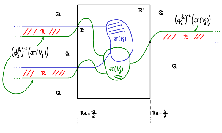
Figure 9. The projection to $\mathbb{C}$ of $V_{i}$, $V_{j}$, $\phi_{t}^{\bar{h}}(V_{j})$ and the regions $R$, $Q$.

Claim 2. $v^{\prime}(S_{r})\cap Q=\emptyset$.

To see this, first note that all connected components of $Q$ are unbounded, hence none of them has compact closure. Now assume by contradiction that $v^{\prime}(S_{r})$ intersects $Q$. Let $Q_{0}$ be one of the connected components of $Q$ that intersects $v^{\prime}(S_{r})$. Note that $v^{\prime}(\partial S_{r})\subset B^{\prime}\cup R$ hence $v^{\prime}(\partial S_{r})\cap Q_{0}=\emptyset$. Note also that all the chords corresponding to the ends of $v^{\prime}$ are disjoint from $Q_{0}$, hence $(\overline{v^{\prime}(S_{r})}\setminus v^{\prime}(S_{r}))\cap Q_{0}=\emptyset$. Finally, $\overline{v^{\prime}(S_{r})}$ is clearly compact. Thus we can apply Proposition 3.3.1 with $w=v^{\prime}$, $\Sigma=S_{r}$, $\Gamma=\mathbb{C}$ and $U=Q_{0}$ and obtain that $\overline{Q}_{0}$ is compact. A contradiction. This concludes the proof of Claim 2.

Note that the intersection points between $\pi(V_{i})\cap(\mathbb{C}\setminus\textnormal{Int\,}B^{\prime})$ and $\pi(\phi_{t}^{h}(V_{j}))\cap(\mathbb{C}\setminus\textnormal{Int\,}B^{\prime})$ are all in $\mathcal{I}$.

Claim 3. Let $P\in\mathcal{I}$. Then for every $z\in\textnormal{Int\,}(S_{r})$, $v^{\prime}(z)\neq P$.

Indeed, if there were a point $z$ with $v^{\prime}(z)=P$, then as $v^{\prime}$ is holomorphic in a neighborhood of $z$ the open mapping would imply that there is a neighborhood of $P$ which is contained in the image of $v^{\prime}$. But Any neighborhood of $P$ must intersect $Q$, hence we obtain a contradiction to Claim 2. This concludes the proof of Claim 3.

We are now ready to prove the main statement of the Auxiliary Lemma, i.e. $\textnormal{image\,}(v^{\prime})\subset B^{\prime}$. By what we have proved so far, it is enough to show that $\textnormal{image\,}(v^{\prime})\cap R=\emptyset$ which we now proceed to show. Indeed, suppose by contradiction that $\textnormal{image\,}(v^{\prime})\cap R\neq\emptyset$. As all the Hamiltonian chords corresponding to $v$ are inside $B^{\prime}\times M$ we have only two possibilities:

1. $\textnormal{image\,}(v^{\prime})\subset\mathcal{R}\cup\mathcal{I}$ and $\textnormal{image\,}(v^{\prime})$ is not constant at one of the points of $\mathcal{I}$.

2. There exists $z_{0},z_{1}\in S_{r}$ with $v^{\prime}(z_{0})\in R$ and $v^{\prime}(z_{1})\in B^{\prime}\setminus\mathcal{I}$.

We begin by ruling out possibility 2. Let $\{z_{t}\}_{t\in[0,1]}$ be a path in $S_{r}$ connecting $z_{0}$ to $z_{1}$ and such that $z_{t}\in\textnormal{Int\,}(S_{r})$ for every $0<t<1$. As

$$\partial B^{\prime}\cap\partial R\subset\mathcal{I}$$

it follows that there exists $0<t_{0}<1$ such that $v^{\prime}(z_{t_{0}})\in\mathcal{I}$. However, this contradicts the Claim 3. This rules out possibility 2.

Assume now that possibility 1 occurs. Then $\textnormal{image\,}(v^{\prime})$ is entirely contained inside $\overline{R_{0}}$, where $R_{0}\subset R$ is one of the connected components. Now $\overline{R_{0}}=R_{0}\cup\{P\}$, where $P\in\mathcal{I}$. Without loss of generality assume that $P=(-\tfrac{3}{2},q)$ for some $q\in\mathbb{Z}$ (the case $P=(\tfrac{5}{2},q)$ can be dealt with in an analogous way). Note that all the Hamiltonian chords that lie in $\overline{R_{0}}\times M$ project via $\pi$ to the point $P$. In particular, at the exit puncture of $S_{r}$, the map $v^{\prime}$ tends to $P$, i.e.

(29) $$\lim_{s\to\infty}v^{\prime}(\epsilon_{k+1}(s,t))=P.$$

Put $v^{\prime\prime}=v^{\prime}\circ\epsilon_{k+1}:[0,\infty)\times[0,1]\to\mathbb{C}$. We have $v^{\prime\prime}(s,0)\in(-\infty,\tfrac{3}{2}]\times\{q\}$ for every $s\geq 0$. We claim that for every $s\geq 0$ we have $\partial_{s}v^{\prime\prime}(s,0)\leq 0$. Indeed, if $\partial_{s}v^{\prime\prime}(s_{0},0)>0$ for some $s_{0}\geq 0$ then as $v^{\prime\prime}$ is holomorphic we have $\partial_{t}v^{\prime\prime}(s_{0},0)=i\partial_{s}v^{\prime\prime}(s_{0},0)\in i\mathbb{R}_{\geq 0}$. It follows that for $t$ close enough to $0$, $v^{\prime\prime}(s_{0},t)\in Q$. But this contradicts the statement at Claim 2. Thus, $\partial_{s}v^{\prime\prime}(s,0)\leq 0$ for every $s\geq 0$. On the other hand we have $\lim_{s\to\infty}v^{\prime\prime}(s,0)=P$. It follows that $v^{\prime\prime}(s,0)=P$ for every $s\geq 0$. From this it is not hard to see (e.g. by a reflection argument) that $v^{\prime\prime}$ is the constant map at $P$. A contradiction. This rules out possibility 1, and concludes the proof of the Auxiliary Lemma.

We now return to the proof of Lemma 3.3.2. Let $C=C_{V_{1},\ldots,V_{k+1}}>0$ to be a large enough constant so that the subset $B=[-\tfrac{3}{2},\tfrac{5}{2}]\times[-C,C]$ satisfies

$$B\supset\bigcup_{\tau\in[0,1]}\phi_{\tau}^{h}(B^{\prime}),$$

where $B^{\prime}$ is the subset in the Auxiliary Lemma. For every $r\in\mathcal{R}^{k+1}$ and every solution $u:S_{r}\to\mathbb{C}\times M$ of (24) we have $\textnormal{image\,}(u)\subset B\times M$.

Indeed, if $u$ is such a solution and we define $v$ using (25) then by the Auxiliary Lemma we have

$$v(z)\in B^{\prime}\times M,\;\forall z\in S_{r}.$$

It follows that

$$u(z)=\phi_{a_{r}(z)}^{\bar{h}}(v(z))\in\phi_{a_{r}(z)}^{h}(B^{\prime})\times M\subset B\times M,\;\forall z\in S_{r}.$$

∎

To be able to apply Gromov compactness to the moduli spaces of solutions of (24) we also need to have some apriori energy estimates that we now proceed to establish.

Let $\mathcal{M}(\gamma_{1},\ldots,\gamma_{k+1};\mathscr{D})$ be the space of pairs $(r,u)$ with $r\in\mathcal{R}^{k+1}$ and $u:S_{r}\to\widetilde{M}$ a solution of the equation (24) with asymptotic conditions at the punctures prescribed by the chords $\gamma_{1},\ldots,\gamma_{k+1}$. Here $\mathscr{D}=\mathscr{D}_{V_{1},\ldots,V_{k+1}}=(\Theta,\mathbf{J})$ is a perturbation datum as described in §3.2.

Recall that the energy of a map $u:S_{r}\to\widetilde{M}$ is defined as follows. Pick a volume form $\sigma$ on $S_{r}$. Let $Y$ be the $1$-form on $S_{r}$ with values in Hamiltonian vector fields associated to $\Theta$. Then

$$E(u):=\tfrac{1}{2}\int_{S_{r}}|Du-Y|_{\mathbf{J}}^{2}\sigma.$$

Recall also that the energy is independent of the form $\sigma$ (note that the norm $|\cdot|_{J}$ on $1$-forms on $S_{r}$ does depend on $\sigma$).

Lemma 3.3.3.

There exists a constant, $C$, depending on the transition functions $\mathbf{a}$, the Hamiltonians $H_{V_{1},V_{2}},\ldots,H_{V_{k},V_{k+1}},H_{v_{1},V_{k+1}}$, $h$ and the perturbation data $\mathscr{D}$ so that for any Hamiltonian chords $\gamma_{1},\ldots,\gamma_{k+1}$ and every $(r,u)\in\mathcal{M}(\gamma_{1},\ldots,\gamma_{k+1};\mathscr{D})$ we have

$$E(u)\leq\int_{S_{r}}u^{*}\widetilde{\omega}+C.$$

Proof.

Let $r\in\mathcal{R}^{k+1}$ and a $u:S_{r}\to\mathbb{C}\times M$ a solution of (24).

Let $s+it$ be local conformal coordinates on $S_{r}$. We write the form $\sigma$ in these coordinates as $\sigma=\lambda ds\wedge dt$, where $\lambda$ is a real function defined locally in the chart of the coordinates $(s,t)$. Write

$$\Theta^{r}_{s,t}=F_{s,t}ds+G_{s,t}dt,$$

where $F_{s,t},G_{s,t}:\widetilde{M}\to\mathbb{R}$ are smooth functions (that depend also on $r\in\mathcal{R}^{k+1}$).

A simple calculation shows that

(30) $$\tfrac{1}{2}|Du-Y|_{\mathbf{J}}^{2}\lambda(s,t)=\widetilde{\omega}(\partial_{s}u,\partial_{t}u)+dF_{s,t}(\partial_{t}u)-dG_{s,t}(\partial_{s}u)-\{F_{s,t},G_{s,t}\}(u(s,t)).$$

Here $\{\cdot,\cdot\}$ is the Poisson bracket, and we use the sign convention that

$$\{F,G\}=-\widetilde{\omega}(X^{F},X^{G})=dF(X^{G}).$$

Denote by $\widetilde{u}:S_{r}\to S_{r}\times\widetilde{M}$ the graph of $u$, $\widetilde{u}(z)=(z,u(z))$. Let $\widetilde{\Theta}^{r}=\textnormal{pr}^{*}\Theta^{r}$, where $\textnormal{pr}:S_{r}\times\widetilde{M}\to\widetilde{M}$ is the projection. We have

$$\widetilde{\Theta}^{r}_{(s,t,p)}=F_{s,t}(p)ds+G_{s,t}(p)dt,\quad\textnormal{where}\,(s,t)\in S_{r},p\in M,$$

$$(\widetilde{u}^{*}\widetilde{\Theta}^{r})_{s,t}=F_{s,t}(u(s,t))ds+G_{s,t}(u(s,t))dt.$$

It follows that

$$d(\widetilde{u}^{*}\widetilde{\Theta}^{r})=\Bigl{(}-\tfrac{\partial F_{s,t}}{\partial t}(u(s,t))+\tfrac{\partial G_{s,t}}{\partial s}(u(s,t))+dG_{s,t}(\partial_{s}u)-dF_{s,t}(\partial_{t}u)\Bigr{)}ds\wedge dt.$$

Substituting this into (30) we obtain:

(31) $$\tfrac{1}{2}|Du-Y|_{\mathbf{J}}^{2}\sigma= u^{*}\widetilde{\omega}-d(\widetilde{u}^{*}\widetilde{\Theta}^{r})$$

$$+\Bigl{(}-\tfrac{\partial F_{s,t}}{\partial t}(u(s,t))+\tfrac{\partial G_{s,t}}{\partial s}(u(s,t))-\{F_{s,t},G_{s,t}\}(u(s,t))\Bigr{)}ds\wedge dt.$$

We start by estimating the integral of the third summand in (31). The estimate here has already been outlined in [Sei3] (see Sections 8g and 9l). It basically follows from the fact that the form $\Theta$ coincides with the Floer datum on the strip like ends (our different choice of $\Theta$ with respect to [Sei3] plays no role in this estimate).

Consider the form $R^{\Theta^{r}}\in\Omega^{2}(S_{r},C^{\infty}(\widetilde{M}))$ defined by $R^{\Theta^{r}}=d\Theta^{r}+\tfrac{1}{2}\{\Theta^{r}\wedge\Theta^{r}\}$, where $d$ stands for the exterior differential on $S_{r}$. In the local coordinates $(s,t)$ we have:

$$R^{\Theta^{r}}_{s,t}=\Bigl{(}-\tfrac{\partial F_{s,t}}{\partial t}+\tfrac{\partial G_{s,t}}{\partial s}-\{F_{s,t},G_{s,t}\}\Bigr{)}ds\wedge dt.$$

This form does not depend on the coordinates $(s,t)$. It is in fact the curvature form of the connection on $S_{r}\times\widetilde{M}$ induced by $\Theta^{r}$. See Chapter 8 of [MS1] for more details. (But note that we use here different sign conventions for Hamiltonian vector fields and for the Poisson bracket. Note also that our $\widetilde{M}$ is $\mathbb{C}\times M$, whereas the $\widetilde{M}$ in [MS1] corresponds in our case to $S_{r}\times\mathbb{C}\times M$.)

Using the curvature $R^{\Theta^{r}}$ we can write the third summand in (31) as

(32) $$\int_{S_{r}}R^{\Theta^{r}}(u).$$

Note that the form $R^{\Theta^{r}}$ vanishes identically over the part of the strip-like ends $\mathcal{W}_{r}\subset S_{r}$. This follows from the fact that $\Theta^{r}$ coincides with $\bar{H}_{V_{i},V_{i+1}}dt$ on $U^{r}_{i}\subset S_{r}$, $i=1,\ldots,k$, and with $\bar{H}_{V_{1},V_{k+1}}dt$ on $U^{r}_{k+1}\subset S_{r}$, where $(s,t)$ are conformal coordinates adapted to the strip-like ends. Moreover, due to the consistency of the family of forms $\Theta$ with respect to gluing/splitting, the forms $\Theta^{r}$ and $R^{\Theta^{r}}$, $r\in\mathcal{R}^{k+1}$, extend continuously in $r\in\overline{\mathcal{R}}^{k+1}$ to the partial compactification $\overline{\mathcal{S}}^{k+1}$ of $\mathcal{S}^{k+1}$.

The extended form $R^{\Theta}$ vanishes identically in a small neighborhood $\mathcal{W}$ of the union of all the punctures of the surfaces in $\overline{S}^{k+1}$. Note that $\overline{S}^{k+1}\setminus\mathcal{W}$ is compact. It follows that for every compact subset $K\subset\mathbb{C}\times M$ there exists a constant $C_{K}$ for which we have the following uniform bound:

$$\int_{S_{r}}\max_{p\in K}R^{\Theta^{r}}(p)\leq C_{K},\quad\forall r\in\overline{\mathcal{R}}^{k+1}.$$

By Lemma 3.3.2, there exists a compact subset $B\subset\mathbb{C}$ (that does not depend on $(r,u)$), such that $u(S_{r})\subset B\times M$. It follows that

$$\int_{S_{r}}R^{\Theta^{r}}(u)\leq\int_{S_{r}}\max_{p\in B\times M}R^{\Theta^{r}}(p)\leq C_{B\times M}.$$

This provides a uniform bound (independent of $(r,u)$) for the integral of the third summand of (31).

We now turn to bounding the integral of the second summand in (31). Here there are some differences in comparison to [Sei3] due to our choice of the form $\Theta$. We have:

(33) $$\int_{S_{r}}-d(\widetilde{u}^{*}\widetilde{\Theta}^{r})= -\int_{\partial S_{r}}\widetilde{u}^{*}\widetilde{\Theta}^{r}$$

$$+\sum_{i=1}^{k}\int_{0}^{1}\bar{H}_{V_{i},V_{i+1}}(t,\gamma_{i}(t))dt-\int_{0}^{1}\bar{H}_{V_{1},V_{k+1}}(t,\gamma_{k+1}(t))dt.$$

As all the Hamiltonian chords $\gamma_{i}$ lie entirely inside the compact subset $B_{V_{1},\ldots,V_{k+1}}\times M$ (see Lemma 3.3.2, the last two terms in (33) are uniformly bounded by a bound that depends only on the maximum of $|\bar{H}_{V_{i},V_{i+}}(t,p)|$ and $|\bar{H}_{V_{1},V_{k+1}}(t,p)|$ over the compact set $[0,1]\times B_{V_{1},\ldots,V_{k+1}}\times M$.

It remains to bound (uniformly in $r$) the first term in (33), namely $\int_{\partial S_{r}}\widetilde{u}^{*}\widetilde{\Theta}^{r}$. (As remarked above, in contrast to our case, in the setting of [Sei3] this term vanishes because $\Theta$ is assumed in [Sei3] to vanish on $T(\partial S_{r})$.)

Recall that $\Theta^{r}=\Theta^{r}_{0}+da_{r}\otimes\bar{h}$ and that $\Theta^{r}_{0}(\xi)=0$ for every $\xi\in T(\partial S_{r})$. Thus we have:

(34) $$\int_{\partial S_{r}}\widetilde{u}^{*}\widetilde{\Theta}^{r}=\int_{\partial S_{r}}\Theta^{r}(u)=\int_{\partial S_{r}}\bar{h}(u)da_{r}.$$

Put $C_{\bar{h}}=\max_{p\in B_{V_{1},\ldots,V_{k+1}}\times M}|\bar{h}(p)|$. By Lemma 3.3.2 we have $|\bar{h}(u(z))|\leq|C_{\bar{h}}|$ for every $z\in S_{r}$. It now follows from Lemma 3.1.1 and (23) that

$$\Bigl{|}\int_{\partial S_{r}}\widetilde{u}^{*}\widetilde{\Theta}^{r}\Bigr{|}\leq C_{\bar{h}}C^{k}_{\mathbf{a}}A_{k+1}.$$

This yields a uniform bound for the integral of the second summand in (31), and concludes the proof of the lemma. ∎

It remains to bound the symplectic area of the solutions of (24). For this we make use of condition (8).

Lemma 3.3.4.

Let $(r,u),(r^{\prime},u^{\prime})\in\mathcal{M}(\gamma_{1},\ldots,\gamma_{k},\gamma_{k+1};\mathscr{D})$. Then

$$\int_{S_{r}}u^{*}\widetilde{\omega}-\int_{S_{r^{\prime}}}u^{\prime*}\widetilde{\omega}=\rho(\mu(u)-\mu(u^{\prime}))$$

where $\mu$ is the Maslov index and $\rho$ is the monotonicity constant.

Proof.

We start with the case when the inclusions $\pi_{1}(V_{i})\to\pi_{1}(\mathbb{C}\times M)$ are all null. We will then modify the argument to cover the case when the image of these inclusions is torsion and under the additional assumption that $c_{1}$, $\int\omega$ are proportional on $H_{2}(M;\mathbb{Z})$. The argument is essentially the same as the one originally used by Oh [Oh1] for strips. We first glue $u$ and $-u^{\prime}$ along the chords $\gamma_{i}$. This produces a surface $N$ of genus $0$ with boundary components $\partial_{i}N$, $1\leq i\leq k+1$, together with a map $j:N\to\mathbb{C}\times M$ whose image is the union of the closures of the images of $u$ and $u^{\prime}$ and whose $i$-th boundary component is mapped to $u(C_{i})\cup u^{\prime}(C_{i})\subset V_{i}$. We now use trivializations of $T(\mathbb{C}\times M)$ over $u$ and $u^{\prime}$ to get a trivialization $\xi$ of $j^{\ast}T(\mathbb{C}\times M)$ and we compute

$$\mu(u)-\mu(u^{\prime})=\mu_{\xi}(\partial_{k+1}N)-\sum_{i=1}^{k}\mu_{\xi}(\partial_{i}N)~{}.~{}$$

This difference can also be computed using other trivializations of $T(\mathbb{C}\times M)$ over $N$. Such trivializations are not unique but it is easy to see that the difference above is independent of this choice.

By (8) $[\partial_{i}N]=0\in\pi_{1}(M)$ for all $i$. Notice that $N$ is homeomorphic to a sphere $S^{2}$ with $k+1$ disjoint disks removed from it. Let $\Gamma_{i}$, $1\leq i\leq k+1$ be $k+1$ copies of the $2$- disk. Consider the surface $N^{\prime}=N\cup_{i=1}^{k+1}\cup_{\partial_{i}N}\Gamma_{i}$. In other words, $N^{\prime}$ is obtained by gluing the disks $\Gamma_{i}$ to $N$ along the boundary components $\partial_{i}N$. Clearly, $N^{\prime}$ is homeomorphic to a sphere.

We now notice that the map $j:N\to M$ extends to a map $x:N^{\prime}\to M$. We fix a trivialization $\theta$ of $x^{\ast}T(\mathbb{C}\times M)$. We restrict this trivialization to $N$ and we get:

$$\mu(u)-\mu(u^{\prime})=\mu_{\xi}(\partial_{k+1}N)-\sum_{i=1}^{k}\mu_{\xi}(\partial_{i}N)=\mu_{\theta}(\partial_{k+1}N)-\sum_{i=1}^{k}\mu_{\theta}(\partial_{i}N)~{}.~{}$$

On the other hand $\mu_{\theta}(-)$ can also be calculated using the disks $\Gamma_{i}$, $1\leq i\leq k+1$, and $x$ (as the trivialization $\theta$ restricts to trivializations of the $\Gamma_{i}$) and so we have, by uniform monotonicity $\mu_{\theta}(\partial_{i}N)=\mu(\Gamma_{i})=\frac{1}{\rho}(\omega_{0}\oplus\omega)(\Gamma_{i})$, $1\leq i\leq k$, and $\mu_{\theta}(\partial_{k+1}N)=2c_{1}(x)-\mu(\Gamma_{k+1})=\frac{1}{\rho}((\omega_{0}\oplus\omega)(x)-(\omega_{0}\oplus\omega)(\Gamma_{k+1}))$. We obtain:

(35) $$\mu(u)-\mu(u^{\prime})=\frac{1}{\rho}((\omega_{0}\oplus\omega)(x)-\sum_{i=1}^{k+1}(\omega_{0}\oplus\omega)(\Gamma_{i}))=$$

$$=\frac{1}{\rho}(\omega_{0}\oplus\omega)(N)=\frac{1}{\rho}((\omega_{0}\oplus\omega)(u)-(\omega_{0}\oplus\omega)(u^{\prime}))$$

It now remains to consider the case when the inclusions $\pi_{1}(V_{i})\to\pi_{1}(\mathbb{C}\times M)$ are torsion but additionally $c_{1}$ and $\int\omega$ are proportional on $H_{2}(M;\mathbb{Z})$. Let $l\in\mathbb{N}$ be big enough so that $l\cdot[\partial_{i}N]=0$ in $\pi_{1}(\mathbb{C}\times M)$, $\forall i$. Let $\widetilde{\Gamma}_{i}\in\pi_{2}(\mathbb{C}\times M,V_{i})$ so that $\partial\widetilde{\Gamma}_{i}=l\cdot\partial_{i}N$. Define the singular chain in $\mathbb{C}\times M$

$$\widetilde{x}=l\cdot N+\sum_{i=1}^{k+1}\widetilde{\Gamma}_{i}~{}.~{}$$

Notice that this is a cycle and thus we can write:

(36) $$l(\mu(u)-\mu(u^{\prime}))=\frac{1}{\rho}((\omega_{0}\oplus\omega)(\widetilde{x})-\sum_{i=1}^{k+1}(\omega_{0}\oplus\omega)(\widetilde{\Gamma}_{i}))=$$

$$=\frac{1}{\rho}(\omega_{0}\oplus\omega)(l\cdot N)=\frac{l}{\rho}((\omega_{0}\oplus\omega)(u)-(\omega_{0}\oplus\omega)(u^{\prime}))$$

∎

Let now $\mathcal{M}_{\nu}(\gamma_{1},\ldots,\gamma_{k},\gamma_{k+1};\mathscr{D})\subset\mathcal{M}(\gamma_{1},\ldots,\gamma_{k},\gamma_{k+1};\mathscr{D})$ be the moduli space formed by those $u$’s with $\mu(u)=\nu$. It follows from the previous lemma that all elements in

$$\mathcal{M}_{\nu}(\gamma_{1},\ldots,\gamma_{k},\gamma_{k+1};\mathscr{D})$$

have the same $\widetilde{\omega}$-area, hence by Lemma 3.3.3 the energy of such curves $u$ is uniformly bounded. In our applications these are the moduli spaces that will be used and $\nu$ will only take the values $0$ and $1$.

3.4. Transversality

In order to define the Fukaya category $\mathcal{F}uk_{cob}^{d}(\mathbb{C}\times M)$ we need to be able to choose regular Floer data, $\mathscr{D}_{V^{\prime},V^{\prime}}=(\bar{H}_{V,V^{\prime}},J_{V,V^{\prime}})$ as well as regular perturbation data $\mathscr{D}_{V_{1},\ldots,V_{k+1}}=(\Theta,\mathbf{J})$ for all Lagrangian cobordisms involved in the construction.

The basic arguments follow those in [Sei3]. Below we explain how they adapt to our case.

We consider the solutions $u$ of (24) associated to the Floer data $\bar{H}_{V,V^{\prime}}$, $J_{V,V^{\prime}}$ as well as to the perturbation data $\mathscr{D}_{V_{1},\ldots,V_{k+1}}=(\Theta,\mathbf{J})$. By Lemma 3.3.2, these solutions are contained inside the sets $B_{V,V^{\prime}}\times M$ and, respectively, $B_{V_{1},\ldots,V_{k+1}}\times M$. We also have that in the interior of these sets, and away from the strip-like ends, $\bar{H}_{V,V^{\prime}}$, $J_{V,V^{\prime}}$ and respectively $\Theta_{0}$, $\mathbf{J}$ are not restricted. However, the Floer data have to satisfy conditions $ii$, $iii$ and the perturbation data have to satisfy the conditions $ii^{\ast}$ and $iii^{\ast}$ from §3.2. In other words, the admissible perturbations - for the Hamiltonian part as well as the almost complex structure - have to be ”vertical” (or contained in $M$) in a small neighborhood of each of the bottlenecks. To show that the data can be chosen to insure regularity, we first make generic choices of Floer and perturbation data in $M$ so that all curves $u$ with $\pi\circ u$ constant equal to a single bottleneck are regular in $M$ (this means, in particular, to choose generically $H_{V,V^{\prime}}$ and $J_{V,V^{\prime}}$ outside of $K_{V,V^{\prime}}$ and similarly for the vertical part of the forms $\Theta_{0}$ outside of $K_{V_{1},\ldots,V_{k+1}}\times M$ - see the point $ii^{\ast}$ in §3.2 - as well as for the relevant almost complex structures). We claim that such curves $u$ continue to be regular also when viewed in $\mathbb{C}\times M$ . To see this we appeal to the specific form of our bottlenecks, namely to the fact that they correspond to maxima of the function $h_{\pm}$. The linearized operator corresponding to equation (24) at such solutions $u$ split into horizontal and vertical components. By the results of §4.3 (more specifically, Corollary 4.3.2 applied with $f_{1}=\cdots=f_{k+1}=h_{-}$ or $h_{+}$) it follows that the index of the horizontal operator is $0$ and that it is surjective. Since the perturbation data were chosen generically in the fiber the vertical part of the operator is also surjective. Consequently the total linearized operator at solutions $u$ with constant projection at the bottleneck is surjective. This proves regularity for curves $u$ with constant projection at the bottlenecks.

It remains to analyze the moduli spaces of curves that do not project to a constant at a bottleneck. At this point it is useful to consider also the curves $v$ that correspond to $u$ via the transformation (25). Clearly, regularity for $u$ is equivalent to regularity for its corresponding $v$. Note also that $u$ projects to a constant at a bottleneck iff its corresponding $v$ has the same property. Now, if $v$ does not project to a constant at a bottleneck then its projection can not remain only in a small neighborhood of any fixed bottleneck: otherwise $\pi\circ v$ would have the same fixed bottleneck point as entry as well as exit which in turn shows that $\pi\circ v$ is constant (indeed, it is easy to see by an application of the open mapping theorem that a bottleneck can only be an exit if the curve $\pi\circ v$ is constant). Thus, these curves reach the region where all the data can be chosen freely. The arguments from [Sei3] together with the standard regularity argument (as for instance in [MS1]) imply that the Floer and perturbation data can be chosen to be both regular and consistent.

3.5. Summing it up

In view of the compactness results in §3.3 and the regularity properties discussed in §3.4, the construction of the Fukaya $A_{\infty}$ category $\mathcal{F}uk_{cob}^{d}(\mathbb{C}\times M)$ can proceed as in the case covered in [Sei3], with the modifications summarized in §2.5 for the monotone setting. As in [Sei3], this process actually leads to a coherent system of $A_{\infty}$-categories. In our case, the categories in this system also depend on the choice of transition functions $\mathbf{a}$ as well as on the function $h$. However, as described in [Sei3] this dependence can be dealt with and the resulting $A_{\infty}$ categories are all quasi-equivalent. In particular, the associated homology categories are all equivalent in a canonical way. These invariance properties will be made explicit in the next section.

For the convenience of the reader, we collect below the main ingredients in the construction of this category and fix relevant notation.

A. Objects

The objects of $\mathcal{F}uk_{cob}^{d}(\mathbb{C}\times M)$ are the Lagrangian cobordisms $V\in\mathcal{CL}_{d}(M)$ (those cobordisms $V\subset\mathbb{C}\times M$, as given in Definition 2.2.1, which are uniformly monotone with monotonicity constant $\rho>0$ and with the number $d_{V}=d\in\mathbb{Z}_{2}$).

B. Morphisms

To define the morphisms we assume regular Floer data $(\bar{H}_{V,V^{\prime}},J_{V,V^{\prime}})$ fixed for any pair $V,V^{\prime}\in\mathcal{CL}_{d}(M)$ - subject to the conditions in §3.2 - and we put

$$\hom(V,V^{\prime})=CF(V,V^{\prime};\bar{H}_{V,V^{\prime}},J_{V,V^{\prime}})=\mathbb{Z}_{2}\langle\mathcal{P}_{V,V^{\prime}}\rangle~{}.~{}$$

C. The Floer complex

The differential $\mu_{1}$ on $C(V,V^{\prime})$, is defined by counting index-$0$ solutions $u:\mathbb{R}\times[0,1]\longrightarrow\widetilde{M}$ of the equation (24), modulo reparametrization by $\mathbb{R}$, in the special case when $k=1$ and $K=dt\otimes\bar{H}_{V,V^{\prime}}$, $J=J_{V,V^{\prime}}$ all over the domain of $u$. The compactness properties in §3.3 obviously apply to this case too and, as a consequence, we deduce that the complex $(C(V,V^{\prime}),\mu_{1})$ satisfies all the usual properties of the standard Lagrangian Floer complex. We denote the resulting Floer homology by $HF(V,V^{\prime})$.

Remark 3.5.1.

Given two cobordisms $V$, $V^{\prime}$ as above as well as the profile function $h:\mathbb{R}^{2}\to\mathbb{R}$, consider the complex $C=CF(V,V^{\prime};(H^{\prime},h);\widetilde{\mathbf{J}})$ as defined in [BC2]. This complex coincides with a complex $CF(V,V^{\prime};\bar{H},\bar{J})$ as defined above for appropriate $\bar{H}$, $\bar{J}$. Thus, for cobordisms, the definition of the Floer complex in the current paper generalizes the one in §4.3 of [BC2]. It is important to note that the particular choice of the shape of the profile function away from $[0,1]\times\mathbb{R}$, in particular the fact that the bottlenecks correspond to local maxima of the functions $h_{\pm}$, implies, as shown in [BC2], that $HF(V,V)\cong QH(V,\partial V)$ (here $QH(V,\partial V)$ is understood without grading and over $\mathbb{Z}_{2}$). This isomorphism was obtained in §5.2 [BC2] by a PSS-argument that makes use of moving boundary conditions. Alternatively, one could use a similar PSS-type morphism

$$PSS:\mathcal{C}(f,J_{V,V})\to CF(V,V;\bar{H}_{V,V},J_{V,V}),$$

where $\mathcal{C}(f,J_{V,V})$ is the pearl complex associated to a function on $V$ whose negative gradient points outward along the boundary of $V$. The advantage of this morphism is that the boundary conditions are now fixed. Either way, by adapting the usual argument from the compact case, it is easy to see that this PSS morphism is compatible with multiplication. Thus the $\mu_{2}$ product on $HF(V,V)$ has a unit because $QH(V,\partial V)$ has as unit the fundamental class of $V$ relative to $\partial V$.

D. The cobordism Fukaya category

Finally, the definition of the higher multiplications, $\mu_{k}$, $k\geq 2$, in $\mathcal{F}uk_{cob}^{d}(\mathbb{C}\times M)$ is given by counting solutions of the equation (24). By Remark 3.5.1 the resulting category is homologically unital.

3.6. Invariance properties of $\mathcal{F}uk^{d}_{cob}(\mathbb{C}\times M)$

Similarly to $\mathcal{F}uk^{d}(M)$, the Fukaya category of cobordisms $\mathcal{F}uk^{d}_{cob}(\mathbb{C}\times M)$ depends on auxiliary choices. The goal of this section is to explain how to compare these different $A_{\infty}$-categories. Recall that the auxiliary choices required in the construction consist of strip-like ends, Floer data for each pair of objects, compatible perturbation data as well as one additional choice, specific to our construction, namely the profile function $h:\mathbb{R}^{2}\to\mathbb{R}$ introduced in §3.2.

Given a profile function $h$ we denote by $\mathcal{I}_{cob}^{h}$ the set of all the possible regular auxiliary structures as above, with Floer and perturbation data corresponding to $h$. For $i\in\mathcal{I}_{cob}^{h}$ we write $\mathcal{F}uk^{d}(\mathbb{C}\times M;i,h)$ for the corresponding Fukaya category (the $h$ in $\mathcal{F}uk^{d}(\mathbb{C}\times M;i,h)$ is superfluous since it is already encoded in $i$, but we write it nevertheless).

The main purpose of this section is to prove the following result.

Proposition 3.6.1.

The family of categories $\mathcal{F}uk^{d}_{cob}(\mathbb{C}\times M;i,h)$, $h\in\mathcal{H}$, $i\in\mathcal{I}^{h}_{cob}$ forms a coherent system in the sense of [Sei3]. In particular they are all quasi-equivalent, and in fact quasi-isomorphic.

The proof of this proposition will occupy §3.6.1, §3.6.2, §3.6.3 and §3.6.4 below. We then deal with another invariance issue: our definition of a profile function involves some additional choices that were made to simplify the compactness arguments in the construction of $\mathcal{F}uk_{cob}^{d}(\mathbb{C}\times M)$. Mainly, the real coordinates of the bottlenecks have been fixed at $\frac{3}{2}$ and $\frac{5}{2}$ - see Figure 8. We will show in §3.6.5 an invariance result with respect to this choice. Finally, in §3.6.6 we discuss the action of horizontal Hamiltonian isotopies on the cobordism Fukaya category.

3.6.1. A tot category integrating the profile functions: basic ingredients

For a profile function $h^{0}:\mathbb{R}^{2}\longrightarrow\mathbb{R}$. We denote by $\mathcal{H}(h^{0})$ the set of all profile functions $h:\mathbb{R}^{2}\longrightarrow\mathbb{R}$ which coincide with $h^{0}$ outside of $[-2,3]\times\mathbb{R}$ and have the same bottlenecks as $h^{0}$ (this last condition is automatic in view of our current definition of profile function).

We will now turn the collection of $A_{\infty}$-categories $\mathcal{F}uk^{d}_{cob}(\mathbb{C}\times M;i,h)$, $h\in\mathcal{H}(h^{0})$, $i\in\mathcal{I}_{cob}^{h}$, into a coherent system of $A_{\infty}$-categories in the sense of §A.6. We follow closely the approach from [Sei3] which has been also summarized (for $\mathcal{F}uk^{d}(M)$) in §2.5.1, namely we will construct an $A_{\infty}$-category $\mathcal{F}uk^{d,tot}_{cob}(\mathbb{C}\times M;h^{0})$ which contains all the $\mathcal{F}uk^{d}_{cob}(\mathbb{C}\times M;i,h)$ as full subcategories, and moreover the embeddings $\mathcal{F}uk^{d}_{cob}(\mathbb{C}\times M;i,h)\longrightarrow\mathcal{F}uk^{d,tot}_{cob}(\mathbb{C}\times M;h^{0})$ are all quasi-equivalences.

The construction of $\mathcal{F}uk^{d,tot}_{cob}(\mathbb{C}\times M;h^{0})$ will be analogous to the one used for $\mathcal{F}uk^{d}_{cob}(\mathbb{C}\times M;i,h)$ (as described in §3.1 - §3.5) only that we will need more general perturbation data. Here are the details of the construction.

Fix $k\geq 2$ and $k+1$ cobordisms $V_{1},\ldots,V_{k+1}\in\mathcal{CL}_{d}(\mathbb{C}\times M)$. Fix also $k+1$ profile functions $h_{V_{1},V_{2}},\ldots,h_{V_{k},V_{k+1}},h_{V_{1},V_{k+1}}\in\mathcal{H}(h^{0})$ and regular Floer data $\mathscr{D}_{V_{1},V_{2}},\ldots,\mathscr{D}_{V_{k},V_{k+1}},\mathscr{D}_{V_{1},V_{k+1}}$ so that $\mathscr{D}_{V_{i},V_{i+1}}$ is defined according to the recipe from §3.2 using the profile function $h_{V_{i},V_{i+1}}$, and similarly $\mathscr{D}_{V_{1},V_{k+1}}$ is defined using the profile function $h_{V_{1},V_{k+1}}$.

We would like to define a higher composition

(37) $$\widehat{\mu}_{k}:CF(V_{1},V_{2};\mathscr{D}_{V_{1},V_{2}})\otimes\cdots\otimes CF(V_{k},V_{k+1};\mathscr{D}_{V_{k},V_{k+1}})\longrightarrow CF(V_{1},V_{k+1};\mathscr{D}_{V_{1},V_{k+1}}).$$

To this end, we need to define new perturbation data $\mathscr{P}_{V_{1},\ldots,V_{k+1}}=(\Theta,\mathbf{J},\mathbf{h})$. The first two structures are similar to those in §3.2 and we will indicate the differences later. The third structure $\mathbf{h}$ consists of a family of profile functions $\mathbf{h}=\{h^{r,z}:\mathbb{R}^{2}\to\mathbb{R}\}_{z\in S_{r}}$ parametrized by $r\in\mathcal{R}^{k+1}$, $z\in S_{r}$. The functions $h^{r,z}$ are required to satisfy the following properties for every $r\in\mathcal{R}^{k+1}$:

1. $h^{r,z}\in\mathcal{H}(h^{0})$ for every $z\in S_{r}$.

2. For every $z$ in the $i$’th in-going strip-like end of $S_{r}$ we have $h^{r,z}=h_{V_{i},V_{i+1}}$, $i=1,\ldots,k$, and over the out-going strip-like end we have $h^{r,z}=h_{V_{1},V_{k+1}}$.

Moreover we require the family $\mathbf{h}$ to be compatible with splitting and gluing in an obvious way which involves the corresponding families for lower values of $k$. Note that such families $\mathbf{h}=\{h^{r,z}:\mathbb{R}^{2}\to\mathbb{R}\}_{z\in S_{r}}$ always exist because for every $r\in\overline{\mathcal{R}}^{k+1}$, $z\in S_{r}$ the set of choices for $h_{r,z}$ is the space $\mathcal{H}(h^{0})$ which is contractible, and therefore the arguments from [Sei3] (Sections (9g) and (9i)) easily extend in our case.

From now on, when the value of $r\in\mathcal{R}^{k+1}$ is obvious we will omit the $r$ from the notation and simply write $h^{z}$.

Next we choose a family of $\widetilde{\omega}$-compatible almost complex structures $\mathbf{J}=\{J_{r,z}\}_{r\in\mathcal{R}^{k+1},z\in S_{r}}$ on $\widetilde{M}$ so that $\pi:\widetilde{M}\to\mathbb{C}$ is $(J_{r,z},(\phi_{a_{r}(z)}^{h^{r,z}})_{*}(i))$-holomorphic for every $z\in S_{r}$ outside $K_{V_{1},\ldots,V_{k+1}}\times M$ (we are using here the notation from §3.2).

The forms $\Theta$ are defined in a similar way as in §3.2 via the formula:

$$\Theta|_{z}=da_{r}\otimes\bar{h}^{r,z}+\Theta_{0},\;\;\forall z\in S_{r},$$

where $\Theta_{0}$ is the same as in §3.2.

We will now describe the precise perturbed Cauchy-Riemann equation relevant for defining the operations $\mu_{k}$. Let $\tau\in[0,1]$ and consider the map

$$S_{r}\longrightarrow\textnormal{Ham}(\mathbb{R}^{2}),\quad z\longmapsto\phi_{\tau}^{h^{r,z}}.$$

Denote by $\beta_{\tau}^{r}\in\Omega^{1}(S_{r},C^{\infty}(T\mathbb{R}^{2}))$ the differential of this map, viewed as a $1$-form on $S_{r}$ with values in the space of Hamiltonian vector fields of $\mathbb{R}^{2}$.

Given $r\in\mathcal{R}^{k+1}$ we define a $1$-form $\mathcal{Y}$ on $S_{r}$ with values in the space of Hamiltonian vector fields of $\widetilde{M}$, whose value at $z\in S_{r}$ is given by:

(38) $$\mathcal{Y}_{z}=X^{\bar{h}^{r,z}}da_{r}+\beta^{r}_{a_{r}(z)}+Y_{0},$$

where all the terms on the right hand side are computed at $T_{z}S_{r}$. Here $Y_{0}=X^{\Theta_{0}}$ is the same as in §3.2. Note that if all the profile functions $h_{i,i+1}$ and $h_{1,k+1}$ coincide and the family $\mathbf{h}$ is constant then $\mathcal{Y}$ coincides with the $1$-form $Y$ we had in §3.2.

We now consider the same equation as (24) but with $Y$ replaced by $\mathcal{Y}$, namely:

(39) $$\ u:S_{r}\to\mathbb{C}\times M,\quad Du+J(z,u)\circ Du\circ j=\mathcal{Y}_{z}+J(z,u)\circ\mathcal{Y}_{z}\circ j,\quad u(C_{i})\subset V_{i}~{}.~{}$$

We claim that Lemma 3.3.2 continues to hold for solutions of (39) (possibly with a different constant $C$). The proof of this is similar to the proof of Lemma 3.3.2 and uses the following additional ingredients:

1. $\beta_{\tau}^{r}\equiv 0$ on the strip-like ends.

2. For every $z\in S^{r}$ and $\xi\in T_{z}S_{r}$ the vector field (on $\mathbb{R}^{2}$) $\beta_{\tau}^{r}(\xi)$ vanishes outside of $[-2,3]\times\mathbb{R}$.

3. Instead of the naturality transformation in (25) we now use $u(z)=\phi^{\bar{h}^{r,z}}_{a_{r}(z)}(v(z))$.

4. Being profile functions, the restrictions of each of the functions $h^{r,z}$ to $(-\infty,-1]\times\{i\}$ has a unique critical point at $-\tfrac{3}{2}\times\{i\}$ which is a local maximum and similarly the restriction to $[2,\infty)\times\{i\}$ has a unique critical point at $\tfrac{5}{2}$ which is also a local maximum. Moreover, all the $h^{r,z}$ coincide with the same profile function $h^{0}$ outside of $[-2,3]\times\mathbb{R}$.

The energy estimates from Lemma 3.3.3 can be adjusted to this case too and we obtain a uniform energy bound for all pairs $(r,u)$ with $r\in\mathcal{R}^{k+1}$ and $u$ satisfying equation 39 with prescribed asymptotic conditions at the punctures. The proof of this is similar to the proof of Lemma 3.3.3 only that we have to use a uniform bound on the functions in the family $\mathbf{h}$ and their derivatives. Finally, Lemma 3.3.4 continues to hold without any changes.

The above imply the standard compactness result for the solutions of (39) with prescribed asymptotic conditions and prescribed Maslov index. Namely, the space of solutions is compact up to splitting and bubbling of holomorphic disks and spheres.

In order to define the operations $\widehat{\mu}_{k}$ from (37) we need to choose the perturbation data $\mathscr{P}_{V_{1},\ldots,V_{k+1}}=(\Theta,\mathbf{J},\mathbf{h})$ in a consistent way (with respect to splitting and gluing of the spaces $\mathcal{R}^{k+1}$ and $\mathcal{S}^{k+1}$ for different values of $k$). This is just a straightforward generalization of the case we had earlier (for $\mathcal{F}uk^{d}_{cob}$), when we had only $(\Theta,\mathbf{J})$ together with the fact (explained earlier) that the family of profile functions $\mathbf{h}=\{h^{r,z}:\mathbb{R}^{2}\to\mathbb{R}\}_{z\in S_{r}}$ can be chosen to be compatible with splitting and gluing.

3.6.2. Definition of the tot category

We are now ready to define the $A_{\infty}$-category $\mathcal{F}uk^{d,tot}_{cob}(\mathbb{C}\times M;h^{0})$ following the scheme from [Sei3]. The objects of this category are triples $(V,i,h)$, where $V\in\mathcal{CL}_{d}(\mathbb{C}\times M)$ is a Lagrangian cobordism, $h\in\mathcal{H}(h^{0})$ and $i\in\mathcal{I}_{cob}^{h}$. To describe the morphisms, choose a regular Floer datum $\mathscr{D}_{(V,i,h^{\prime}),(W,j,h^{\prime\prime})}$ for every pair of objects $(V,i,h^{\prime})$, $(W,j,h^{\prime\prime})$, in an arbitrary way but subject to the following two conditions: the Floer datum should be defined using a profile function from $\mathcal{H}(h^{0})$, and moreover, when $(i,h^{\prime})=(j,h^{\prime\prime})$ then the Floer datum should coincide with the one prescribed by the index $i=j$ and profile function $h^{\prime}=h^{\prime\prime}$. The morphism space $\hom\bigl{(}(V,i,h^{\prime}),(W,j,h^{\prime\prime})\bigr{)}$ is then defined as $CF(V,W;\mathscr{D}_{(V,i,h^{\prime}),(W,j,h^{\prime\prime})})$ and the differential $\widehat{\mu}_{1}$ is precisely the same as for the earlier definition of $\mathcal{F}uk^{d}_{cob}(\mathbb{C}\times M)$. Namely, we do not use equation (39) to define $\widehat{\mu}_{1}$, but rather equation (24) (with $S_{r}=\mathbb{R}\times[0,1]$ of course).

The higher order compositions $\widehat{\mu}_{k}$ are defined as follows. We choose regular consistent perturbation data $\mathscr{P}_{V_{1},\ldots,V_{k+1}}=(\Theta,\mathbf{J},\mathbf{h})$ as described above for each $k+1$ tuple of objects $(V_{1},i_{1},h_{1}),\ldots,(V_{k+1},i_{k+1},h_{k+1})$ subject to the condition that when $h_{1}=\cdots=h_{k+1}=h$ and $i_{1}=\cdots=i_{k+1}=i$ then the family of profile functions $\mathbf{h}$ is constant and equals $h$ and $(\Theta,\mathbf{J})$ are the same as prescribed by $i$. The operation $\widehat{\mu}_{k}$ is then defined by counting index-$0$ solutions of (39) in the standard way.

The fact that the operations $\widehat{\mu}_{k}$, $k\geq 1$, satisfy the $A_{\infty}$-identities can be proved in the same way as for the categories $\mathcal{F}uk^{d}_{cob}(\mathbb{C}\times M;i,h)$.

Note that when $\mathbf{h}$ is the constant family (i.e. $h^{r,z}=h$ for every $r,z$) then (38) coincides with the $1$-forms $Y$ and equation (39) becomes the same as (24). It follows that for every $h\in\mathcal{H}(h^{0})$ and $i\in\mathcal{I}_{cob}^{h}$ we have an obvious inclusion

(40) $$\mathcal{F}uk^{d}_{cob}(\mathbb{C}\times M;i,h)\longrightarrow\mathcal{F}uk^{d,tot}_{cob}(\mathbb{C}\times M;h^{0})$$

which is a full and faithful $A_{\infty}$-functor. Note also that similarly to $\mathcal{F}uk^{d}_{cob}(\mathbb{C}\times M;i,h)$ the category $\mathcal{F}uk^{d,tot}_{cob}(\mathbb{C}\times M;h^{0})$ too is homologically unital.

3.6.3. The canonical inclusions are quasi-equivalences.

It remains to show that the inclusions (40) are quasi-equivalences. Let $V,W\in\mathcal{CL}_{d}(\mathbb{C}\times M)$ be two cobordisms. Fix a profile function $h^{0}$ and let $\mathscr{D}=\mathscr{D}_{V,W}$, $\mathscr{D}^{\prime}=\mathscr{D}^{\prime}_{V,W}$ be two arbitrary regular Floer data for $(V,W)$ both constructed using profile functions $h,h^{\prime}\in\mathcal{H}(h^{0})$. Choose a perturbation datum $\mathscr{P}=(\Theta,\mathbf{J},\mathbf{h})$ on the strip $Z=\mathbb{R}\times[0,1]$ which extends $\mathscr{D}$ at the negative end of $Z$ and extends $\mathscr{D}^{\prime}$ at the positive end of $Z$. This perturbation datum $\mathscr{P}$ is constructed exactly as was done above (for $S_{r}$ when $k\geq 2$), only that now it is defined over $Z$.

We define a map

(41) $$\Phi_{\mathscr{P}}:CF(V,W;\mathscr{D})\longrightarrow CF(V,W;\mathscr{D}^{\prime}),\quad\Phi_{\mathscr{P}}(\gamma)=\sum_{\gamma^{\prime}}\#\mathcal{M}_{0}(\gamma,\gamma^{\prime};\mathscr{P})\gamma^{\prime},$$

where $\gamma^{\prime}\in\mathcal{P}_{\bar{H}^{\prime}}$ (i.e. $\gamma^{\prime}$ is a chord of the Hamiltonian $\bar{H}^{\prime}$ (of $\mathscr{D}^{\prime}$) starting on $V$ and ending on $W$) and $\mathcal{M}_{0}(\gamma,\gamma^{\prime};\mathscr{P})$ stands for the $0$-dimensional component of the space of maps $u:Z\to\widetilde{M}$ which satisfy the same equation as (39) with $S_{r}$ replaced by $Z$ and with the boundary and asymptotic conditions replaced by the following:

$$u(\mathbb{R}\times 0)\subset V,\quad u(\mathbb{R}\times 1)\subset W,$$

$$\lim_{s\to-\infty}u(s,t)=\gamma(t),\quad\lim_{s\to\infty}u(s,t)=\gamma^{\prime}(t).$$

The compactness arguments from §3.3 apply to $\mathcal{M}(\gamma,\gamma^{\prime};\mathscr{P})$ and together with standard transversality arguments show that:

1. $\mathcal{M}_{0}(\gamma,\gamma^{\prime};\mathscr{P})$ is a compact $0$-dimensional manifold, hence a finite set. Thus $\Phi_{\mathscr{P}}$ is well defined.

2. $\Phi_{\mathscr{P}}$ is a quasi-isomorphism of chain complexes.

3. The induced map in homology, which we denote by

   $$\Phi_{\mathscr{D}^{\prime},\mathscr{D}}:H(CF(V,W;\mathscr{D}))\longrightarrow H(CF(V,W;\mathscr{D}^{\prime})$$

   is independent of $\mathscr{P}$. Moreover, the maps $\Phi_{\mathscr{D}^{\prime},\mathscr{D}}$ (for different $\mathscr{D}$, $\mathscr{D}^{\prime}$) together with the product $\mu_{2}$ satisfy the TQFT composition laws (as described in Section 8b in [Sei3]). In particular, these maps are compatible with the triangle product.

We call the maps $\Phi_{\mathscr{P}}$ as well as $\Phi_{\mathscr{D}^{\prime},\mathscr{D}}$, continuation maps or comparison maps.

Next we consider the special case $(V,V)$, i.e. $W=V$. Let $\mathscr{D}$, $\mathscr{D}^{\prime}$, $\mathscr{D}^{\prime\prime}$ be three Floer data for the pair $(V,V)$, all constructed using profile function from $\mathcal{H}(h^{0})$. By choosing a perturbation datum $\mathcal{P}_{\mathscr{D}^{\prime},\mathscr{D}^{\prime},\mathscr{D^{\prime\prime}}}$ on $S_{3}$, which is compatible with these three Floer data (as described above) we obtain the triangle product:

$$\widehat{\mu}_{2}:CF(V,V;\mathscr{D})\otimes CF(V,V;\mathscr{D}^{\prime\prime})\longrightarrow CF(V,V;\mathscr{D}^{\prime}).$$

We denote the induced map in homology by

$$*:HF(V,V;\mathscr{D})\otimes HF(V,V;\mathscr{D}^{\prime\prime})\longrightarrow HF(V,V;\mathscr{D}^{\prime}).$$

The isomorphism $\Phi_{\mathscr{D}^{\prime},\mathscr{D}}$ can be expressed via the product $*$. More precisely, there exists a canonical element $u\in HF(V,V;\mathscr{D}^{\prime\prime})$ such that

(42) $$\Phi_{\mathscr{D}^{\prime},\mathscr{D}}(a)=a*u,\;\;\forall a\in HF(V,V;\mathscr{D}).$$

The element $u$ can be described as follows. Let $PSS:QH(V,\partial V)\to HF(V,V;\mathscr{D}^{\prime\prime})$ be the PSS isomorphism as described e.g. in Section 5.2 of [BC2]. Recall that $QH(V,\partial V)$ has a well defined unity $[V]$. The element $u$ is then defined by $u=PSS([V])$. The proof of (42) is similar to the case of closed Lagrangian submanifolds. It basically follows from the fact that $\Phi_{\mathscr{D}^{\prime},\mathscr{D}}$ is compatible with the $\mu_{2}$-product and the TQFT composition identities (see e.g. [Sei3] Section 8b). These extend to our setting due to the compactness arguments from §3.3. Alternatively, one can construct $u\in HF(V,V;\mathscr{D}^{\prime\prime})$ by counting perturbed holomorphic maps $D\setminus\{1\}\to\mathbb{C}\times M$ from a disk punctured at one point, where the perturbation extends the Floer datum $\mathscr{D}^{\prime\prime}$ on the strip-like end corresponding to the puncture $1\in D$. (See Section 8l of [Sei3] for more on that.)

It follows that for every $V\in\mathcal{C}\mathcal{L}_{d}(\mathbb{C}\times M)$, and $h^{\prime},h^{\prime\prime}\in\mathcal{H}(h^{0})$, $i^{\prime}\in\mathcal{I}_{cob}^{h^{\prime}}$, $i^{\prime\prime}\in\mathcal{I}_{cob}^{h^{\prime\prime}}$ the objects $(V,i^{\prime},h^{\prime})$ and $(V,i^{\prime\prime},h^{\prime\prime})$ are isomorphic in the homological category $H\mathcal{F}uk_{cob}^{d,tot}(\mathbb{C}\times M);h^{0})$. Standard results in homological algebra [GM] imply that the homological embeddings

$$H\mathcal{F}uk^{d}_{cob}(\mathbb{C}\times M;i,h)\longrightarrow H\mathcal{F}uk^{d,tot}_{cob}(\mathbb{C}\times M;h^{0}),$$

associated to (40), are equivalences for every $i$ and $h$. By the discussion in §A.6 (see also [Sei3] for more details) this gives the family $\mathcal{F}uk_{cob}^{d}(\mathbb{C}\times M;i,h)$, $h\in\mathcal{H}(h^{0})$, $i\in\mathcal{I}_{cob}^{h}$, the structure of a coherent system of $A_{\infty}$-categories. In particular we obtain for every $h^{\prime},h^{\prime\prime}\in\mathcal{H}(h^{0})$ and $i^{\prime}\in\mathcal{I}_{cob}^{h^{\prime}}$, $i^{\prime\prime}\in\mathcal{I}_{cob}^{h^{\prime\prime}}$ a quasi-equivalence

(43) $$\mathcal{F}_{(i^{\prime\prime},h^{\prime\prime}),(i^{\prime},h^{\prime})}:\mathcal{F}uk_{cob}^{d}(\mathbb{C}\times M;i^{\prime},h^{\prime})\longrightarrow\mathcal{F}uk_{cob}^{d}(\mathbb{C}\times M;i^{\prime\prime},h^{\prime\prime})$$

which is canonical in homology and satisfies $\mathcal{F}_{(i^{\prime\prime},h^{\prime\prime}),(i^{\prime},h^{\prime})}(V)=V$ for every object $V$. (In fact $\mathcal{F}_{(i^{\prime\prime},h^{\prime\prime}),(i^{\prime},h^{\prime})}$ is a quasi-isomorphism.) Moreover, for every two cobordisms $V$ and $W$, the action of the degree $1$ component of $\mathcal{F}_{(i^{\prime\prime},h^{\prime\prime}),(i^{\prime},h^{\prime})}$ on morphisms, namely $\mathcal{F}^{V,W}_{(i^{\prime\prime},h^{\prime\prime}),(i^{\prime},h^{\prime})}:CF(V,W;\mathscr{D}^{\prime})\to CF(V,W;\mathscr{D}^{\prime\prime})$, coincides in homology with the continuation map $\Phi_{\mathscr{D}^{\prime\prime},\mathscr{D}^{\prime}}$. Here $\mathscr{D}^{\prime}$, $\mathscr{D}^{\prime\prime}$, are the Floer data for $(V,W)$ corresponding to the choices $i^{\prime}$ and $i^{\prime\prime}$ respectively.

3.6.4. Changing the profile function at infinity.

Summarizing the construction till now, we have an $A_{\infty}$-category $\mathcal{F}uk^{d}_{cob}(\mathbb{C}\times M;h)$ which is well defined up to quasi-isomorphism, but still depends on the choice of the profile function at $\pm\infty$. It remains to get rid of this dependence.

Denote by $\mathcal{H}$ the space of all profile functions (with all possible constants $\alpha^{\pm}$, $\beta^{\pm}$, but subject to the conditions described in §3.2, in particular $\alpha^{-}>0$, $\alpha^{+}<0$ etc.). Let $h^{0},h^{1}\in\mathcal{H}$. Denote by $\alpha^{\pm}_{i}$, $i=0,1$, the constants defining $h^{i}$ on $(-\infty,2]\times\mathbb{R}$ and $[3,\infty)\times\mathbb{R}$. Fix $0<\epsilon<1/100$ and choose a function $\sigma:\mathbb{R}\to\mathbb{R}$ with the following properties:

1. $\sigma(x)=1$ for every $x\in[-\tfrac{3}{2}-\epsilon,\tfrac{5}{2}+\epsilon]$.

2. $\sigma(x)=\tfrac{\alpha_{1}^{-}}{\alpha_{0}^{-}}$ for $x\leq-2$ and $\sigma(x)=\tfrac{\alpha_{1}^{+}}{\alpha_{0}^{+}}$ for $x\geq 3$.

Using this function we can construct a bijection

$$\tau_{h^{1},h^{0}}:\mathcal{H}(h^{0})\longrightarrow\mathcal{H}(h^{1})$$

which is uniquely characterized by the following property. For every $h\in\mathcal{H}(h^{0})$

(44) $$(\tau_{h^{1},h^{0}}h)(x,i)=h(x,i),\quad\forall x\in[-\tfrac{3}{2}-\epsilon,\tfrac{5}{2}+\epsilon],i\in\mathbb{Z},$$

$$\frac{\partial(\tau_{h^{1},h^{0}}h)}{\partial x}(x,i)=\sigma(x)\frac{\partial h}{\partial x}(x,i),\quad\forall x\in\mathbb{R},i\in\mathbb{Z}.$$

For every $h\in\mathcal{H}(h^{0})$, the bijection $\tau_{h^{1},h^{0}}$ induces in an obvious way a bijection $\tau_{h^{1},h^{0}}:\mathcal{I}_{cob}^{h}\longrightarrow\mathcal{I}_{cob}^{\tau_{h^{1},h^{0}}h}$ which we also denote by $\tau_{h^{1},h^{0}}$. Note that the Hamiltonian chords corresponding to $i\in\mathcal{I}_{cob}^{h}$ and to $\tau_{h^{1},h^{0}}i\in\mathcal{I}_{cob}^{\tau_{h^{1},h^{0}}h}$ coincide. Moreover, due to (44) and in view of Lemma 3.3.2 the equation (24) has precisely the same solutions for the choice of data $i$ and $\tau_{h^{1},h^{0}}i$. Thus the $A_{\infty}$-categories $\mathcal{F}uk^{d}_{cob}(\mathbb{C}\times M;i;h)$ and $\mathcal{F}uk^{d}_{cob}(\mathbb{C}\times M;\tau_{h^{1},h^{0}}i;\tau_{h^{1},h^{0}}h)$ can be identified by an obvious chain-level isomorphism induced from $\tau_{h^{1},h^{0}}$:

$$T^{i,h}_{h^{1},h^{0}}:\mathcal{F}uk^{d}_{cob}(\mathbb{C}\times M;i,h)\longrightarrow\mathcal{F}uk^{d}_{cob}(\mathbb{C}\times M;\tau_{h^{1},h^{0}}i,\tau_{h^{1},h^{0}}h).$$

The action of $T_{h^{1},h^{0}}$ on objects is of course the “identity”.

A slight variation on Lemma 3.3.2 shows that the isomorphisms $T_{h^{1},h^{0}}$ are compatible with the quasi-equivalences (43) in the sense that for every $h^{\prime},h^{\prime\prime}\in\mathcal{H}(h^{0})$ and $i^{\prime}\in\mathcal{I}^{h^{\prime}}_{cob}$, $i^{\prime\prime}\in\mathcal{I}^{h^{\prime\prime}}_{cob}$ we have:

$$T^{i^{\prime\prime},h^{\prime\prime}}_{h^{1},h^{0}}\circ\mathcal{F}_{(i^{\prime\prime},h^{\prime\prime}),(i^{\prime},h^{\prime})}=\mathcal{F}_{(\tau_{h^{1},h^{0}}i^{\prime\prime},\tau_{h^{1},h^{0}}h^{\prime\prime}),(\tau_{h^{1},h^{0}}i^{\prime},\tau_{h^{1},h^{0}}h^{\prime})}\circ T^{i^{\prime},h^{\prime}}_{h^{1},h^{0}}.$$

Finally, it follows from the definitions that the isomorphisms $T^{i,h}_{h^{1},h^{0}}$ have also the following compatibility properties:

$$T^{\tau_{h^{1},h^{0}}i,\tau_{h^{1},h^{0}}h}_{h^{2},h^{1}}\circ T^{i,h}_{h^{1},h^{0}}=T^{i,h}_{h^{2},h^{0}}.$$

This concludes the proof of Proposition 3.6.1. In view of this result we will denote by abuse of notation each of the categories $\mathcal{F}uk^{d}_{cob}(\mathbb{C}\times M;i,h)$ by $\mathcal{F}uk^{d}_{cob}(\mathbb{C}\times M)$. However, notice for further use that each time an explicit geometric construction takes place we generally need to indicate what are the particular choices of almost complex structures, profile functions etc.

Remark 3.6.2.

In the last step in the discussion above we have made a chain level comparison between $\mathcal{F}uk^{d}_{cob}(\mathbb{C}\times M;i,h)$ for certain pairs of functions $h\in\mathcal{H}$ which do not coincide at infinity. There is an alternative way to establish this comparison which in fact generalizes the construction of the quasi-equivalences $\mathcal{F}_{(i^{\prime\prime},h^{\prime\prime}),(i^{\prime},h^{\prime})}$ described above. This goes as follows. One constructs directly an $A_{\infty}$-category $\widehat{\mathcal{F}uk}^{d,tot}_{cob}(\mathbb{C}\times M)$ which is defined in a similar way to $\mathcal{F}uk^{d,tot}_{cob}(\mathbb{C}\times M;h)$, with the following changes. One allows Floer data to have profile functions which do not necessarily coincide at infinity. Moreover, one takes perturbation data $\mathscr{P}=(\Theta,\mathbf{J},\mathbf{h})$, where the family of profile functions $h\in\mathcal{H}$ interpolates the given choices of profile functions on the ends of the punctured disks $S_{r}$. The operations $\widehat{\mu}_{k}$ from (37) are then defined via the same equation (39). The only thing left to be checked is whether compactness holds for the spaces of solutions of (39). It turns out that a rather straightforward generalization of Lemma (3.3.2) holds for these solutions too. The main point is that the constants $\alpha^{\pm}$ (for the different profile functions involved) have the same signs and are small enough.

3.6.5. Independence of bottleneck position.

In this subsection we discuss the independence of the cobordism Fukaya category on the positions along the real axis of the bottlenecks of the profile function. It is clear that our choice to put the bottlenecks at the points $-\frac{3}{2}$ and $\frac{5}{2}$ is completely arbitrary. We get rid of this dependence below.

Denote by $\mathcal{C}\mathcal{L}_{d}^{[a,b]}(\mathbb{C}\times M)$ the Lagrangians in $\mathbb{C}\times M$ that are $\mathbb{R}$-extensions of cobordisms $V\subset[a,b]\times\mathbb{R}\times M$ with $-\infty<a<b<\infty$, that satisfy condition (8) and are uniformly monotone with $d_{V}=d$. For instance, $\mathcal{C}\mathcal{L}^{[0,1]}_{d}(\mathbb{C}\times M)=\mathcal{C}\mathcal{L}_{d}(\mathbb{C}\times M)$. For fixed $c\leq a\leq 0<1\leq b\leq d$ we define a coherent system of categories $\mathcal{F}uk_{[a,b]}^{d}(\mathbb{C}\times M;[c,d])$ by the same method used before in this section to define $\mathcal{F}uk^{d}_{cob}(\mathbb{C}\times M)$. Their role is to integrate all possible bottleneck positions for the profile functions.

The objects of $\mathcal{F}uk_{[a,b]}^{d}(\mathbb{C}\times M;[c,d])$ are the Lagrangians in the set $\mathcal{C}\mathcal{L}_{d}^{[a,b]}(\mathbb{C}\times M)$. The morphisms and the multiplications $\mu_{k}$ are defined just as in our construction of $\mathcal{F}uk^{d}_{cob}(\mathbb{C}\times M)$ but this time we use profile functions $h^{[c,d]}$ similar to the ones considered till now but rescaled to the interval $[c,d]$: thus such an $h^{[c,d]}$ satisfies the properties given in the definition of the function $h$ in §3.2 but relative to the interval $[c,d]$ instead of the interval $[0,1]$. For instance, we use the sets,

$$W_{i}^{+}=[d+1,\infty)\times[i-\epsilon,i+\epsilon]\quad\textnormal{and }\;W_{i}^{-}=(-\infty,-1+c]\times[i-\epsilon,i+\epsilon],\;i\in\mathbb{Z}~{},~{}$$

and the functions $h_{\pm}$ have respectively critical points at $\frac{5}{2}+d$ and $-\frac{3}{2}+c$. In particular, $\mathcal{F}uk^{d}_{cob}(\mathbb{C}\times M)=\mathcal{F}uk^{d}_{[0,1]}(\mathbb{C}\times M;[0,1])$.

It will be shown below that all these categories are in fact quasi-isomorphic. Clearly, there is an inclusion of (coherent systems of) $A_{\infty}$ categories:

$$\widetilde{Id}_{a,b}:\mathcal{F}uk^{d}_{[0,1]}(\mathbb{C}\times M;[c,d])\to\mathcal{F}uk^{d}_{[a,b]}(\mathbb{C}\times M;[c,d]).$$

Proposition 3.6.3.

With the notation above we have:

• Any two cobordisms $V,V^{\prime}\in\mathcal{CL}_{d}^{[a,b]}(\mathbb{C}\times M)$ that are horizontally isotopic are isomorphic in the homological category $H(\mathcal{F}uk^{d}_{[a,b]}(\mathbb{C}\times M);[c,d])$. As a consequence $\widetilde{Id}_{a,b}$ is a quasi-equivalence.

• Any two categories $\mathcal{F}uk_{[a,b]}^{d}(\mathbb{C}\times M;[c,d])$ are canonically quasi-equivalent, independently of $c\leq a\leq 0<1\leq b\leq d$.

Proof.

Point i is very similar to the argument at the beginning of §3.6.3 except that we not only modify the data $\mathscr{D}$ but rather isotope from $V$ to $V^{\prime}$. Suppose that $V$ and $V^{\prime}$ are horizontally isotopic via a horizontal isotopy $\Psi$. As showed in [BC2] there is an associated isomorphism $\overline{\Psi}:HF(V,V)\to HF(V,V^{\prime})$. Let $\alpha=\overline{\Psi}(u)$ where $u\in HF(V,V)$ is, as in §3.6.3, the unit (that is the image of the fundamental class by the PSS-morphism $QH(V,\partial V)\to HF(V,V)$). A similar class $\beta$ can be defined in $HF(V^{\prime},V)$. These classes satisfy $\alpha\ast\beta=u$ and $\beta\ast\alpha=u^{\prime}$ thus showing that $V$ and $V^{\prime}$ are isomorphic in the homology category as claimed. In homology the functor $\widetilde{Id}_{a,b}$ is full and faithful and as any cobordism in $\mathcal{CL}^{[a,b]}_{d}(\mathbb{C}\times M)$ can be rescaled by a horizontal isotopy to $[0,1]\times\mathbb{R}\times M$, it follows from the first part of the proof that $\widetilde{Id}_{a,b}$ is a quasi-equivalence.

We now prove point ii. In view of i, it is clearly enough to prove that given $c\leq 0,1\leq d$ there is a quasi-equivalence of the two categories $\mathcal{F}uk^{d}_{[0,1]}(\mathbb{C}\times M;[0,1])$ and $\mathcal{F}uk^{d}_{[0,1]}(\mathbb{C}\times M;[c,d])$. For this we will use a special ambient hamiltonian isotopy induced by a hamiltonian isotopy in the plane, $\xi_{t}$, with the property that: $\xi_{t}:\mathbb{C}\to\mathbb{C}$ is a translation of the form $(x,y)\to(x+tv_{-},y)$ for $(x,y)\in(-\infty,\epsilon]\times\mathbb{R}$ and $(x,y)\to(x+tv_{+},y)$ for $(x,y)\in[1-\epsilon,\infty)\times\mathbb{R}$ with $\epsilon$ very small and $v_{-}<0$ and $v_{+}>0$. Moreover, the choices of $v_{+}$ and $v_{-}$ are so that some fixed profile function $h_{0}=h^{[0,1]}$ has the property that $h_{0}\circ\xi_{1}^{-1}$ is a profile function of the type $h^{[c,d]}$. We will now construct an appropriate tot category $\mathcal{F}uk^{d}_{[0,1]}(\mathbb{C}\times M)^{\xi}$. The objects of this category are pairs $(V,t)$ where $V\in\mathcal{CL}_{d}^{[0,1]}(\mathbb{C}\times M)$ and $t\in[0,1]$. We now fix Floer and perturbation data for each fixed $t\in[0,1]$ in an arbitrary way except that at each $t$ we use as profile function $h^{t}=h_{0}\circ\xi_{t}^{-1}$. This produces categories $\mathcal{F}uk^{d}_{[0,1]}(\mathbb{C}\times M;h^{t})$. This data, now defined for each fixed value of $t$ has now to be extended to more general families of the form $(V_{i},t_{i})$ with different parameters $t_{i}$. The construction is similar to the construction of the tot category in §3.6.1 and §3.6.2. We first fix the specific class of profile functions that we will use: $\mathcal{H}^{\xi}=\{h^{t}:\ t\in[0,1]\}$. We then use $\mathcal{H}^{\xi}$ instead of $\mathcal{H}(h^{0})$ in the construction in §3.6.1. In particular, we consider families $\bar{h}^{r,z}$ so that conditions i and ii after equation (37) are satisfied with $\mathcal{H}^{\xi}$ instead of $\mathcal{H}(h^{0})$, in particular $h^{r,z}\in\mathcal{H}^{\xi}$ for each $r\in\mathcal{R}^{k+1}$ and $z\in S_{r}$. From here on the construction is just like in §3.6.2: for each pair $(V,t_{1}),(W,t_{2})$ we select Floer data $\mathscr{D}_{(V,t_{1}),(W,t_{2})}$ up to our usual conditions but so that the profile function is selected from $\mathcal{H}^{\xi}$ and, whenever $t_{1}=t_{2}$, the datum and the profile function coincides with the one prescribed for $t_{1}$. We then define the higher compositions for each $k+1$-tuple of objects $(V_{1},t_{1}),\ldots(V_{k+1},t_{k+1})$ in the usual way but subject to the condition that the profile function is a family $\mathbf{h}=\{h^{r,z}\}$ as described above and is so that if $t_{1}=t_{2}=\ldots t_{k+1}$ then $h^{r,z}$ is the constant family equal to $h^{t_{1}}$ and, similarly, the rest of the data coincides with the one in $\mathcal{F}uk^{d}_{[0,1]}(\mathbb{C}\times M;h^{t_{1}})$. On the technical level there are two points to check to finish the construction of $\mathcal{F}uk^{d}_{[0,1]}(\mathbb{C}\times M)^{\xi}$. The first concerns the localization of curves in the relevant moduli spaces - the analogue of Lemma 3.3.2. The second second point is to verify energy bounds as in Lemma 3.3.3. This second point does not present any particular difficulty but the first one requires a new argument. The reason is that the functions $h^{t}$ have bottlenecks at different points along the real axis - these bottlenecks are simply translations along $\mathbb{R}\subset\mathbb{C}$ of the bottlenecks of $h$ but for various values of $t$ these are different points. Thus the reasoning used in §3.6.1 requires an adaptation that we now describe. Consider a solution $u$ of the equation (39) but, of course, with $h^{r,z}\in\mathcal{H}^{\xi}$. Denote by $\psi_{t}$ the lift of $\xi_{t}$ to $\mathbb{C}\times M$. We will again use a naturality transformation $u(z)=\phi_{a_{r}(z)}^{\bar{h}^{r,z}}(v(z))$ (we recall $\bar{h}^{r,z}=h^{r,z}\circ\pi$). In this case $\bar{h}^{r,z}$ can be written as $\bar{h}^{b_{r}(z)}$ where $b_{r}:S_{r}\to[0,1]$ and, further, $\bar{h}^{b_{r}(z)}=\bar{h}_{0}\circ\psi_{b_{r}(z)}^{-1}$. By an elementary calculation we have:

$$\phi_{\tau}^{\bar{h}^{r,z}}={\psi}_{b_{r}(z)}\circ\phi_{\tau}^{\bar{h}_{0}}\circ{\psi}_{b_{r}(z)}^{-1}\ ,\ \forall\tau~{}.~{}$$

We now apply yet another naturality transformation to $v$ by putting

$$w(z)={\psi}_{b_{r}(z)}^{-1}v(z)~{}.~{}$$

We now discuss the properties of the planar maps $w^{\prime}(z)=\pi\circ w(z)$. Because $\xi_{t}$ is a translation (for all $t$) in the real direction in the exterior of the region $[\epsilon,1-\epsilon]$, the holomorphicity of $\pi\circ v$ around and on the sides of the bottlenecks is still true for $w$. Moreover, the boundary conditions for $w$ are such that for $w$ only the bottlenecks of $h_{0}$ itself are involved. In other words, the argument in Lemma 3.3.2 is applicable to $w$ and concludes the verification.

The usual arguments used in the construction of the tot category show that the “fibre” inclusion:

$$\mathcal{F}uk^{d}_{[0,1]}(\mathbb{C}\times M;h^{t})\to\mathcal{F}uk^{d}_{[0,1]}(\mathbb{C}\times M)^{\xi}$$

is a quasi-equivalence for all $t\in[0,1]$ and this implies that the first fibre which is $\mathcal{F}uk^{d}_{[0,1]}(\mathbb{C}\times M;[0,1])$ and the last one which is $\mathcal{F}uk^{d}_{[0,1]}(\mathbb{C}\times M;[c,d])$ are quasi-equivalent. ∎

3.6.6. Action of horizontal Hamiltonian isotopies.

Here we analyze the action of certain Hamiltonian diffeomorphisms $\phi:\mathbb{C}\times M\to\mathbb{C}\times M$ on $\mathcal{F}uk^{d}_{cob}(\mathbb{C}\times M)$. The construction is parallel to a construction in [Sei3], specifically §10d, with some modifications that we will outline. The Hamiltonian diffeomorphisms $\phi$ of interest to us satisfy a strong version of horizontality that we define below.

Definition 3.6.4.

Fix a hamiltonian isotopy $\phi_{t}$ , $t\in[0,1]$, on $\mathbb{C}\times M$. Let $X_{t}$ be the time dependent vector field of $\phi_{t}$. The isotopy $\phi_{t}$ is called an ambient horizontal hamiltonian isotopy if it has the property that there are sufficiently large constant $R_{\phi},R^{\prime}_{\phi}>0$ so that for each $t\in[0,1]$ there are two other real numbers $v^{t}_{-},v^{t}_{+}\in\mathbb{R}$ so that for all $z=(x+iy,m)\in\mathbb{C}\times M$, we have

$$X_{t}(z)=(v^{t}_{-},0)\in\mathbb{C}\oplus T_{m}M\ \textnormal{if \ }x\leq-R^{\prime}_{\phi}\ ,\ X_{t}(z)=(v^{t}_{+},0)\in\mathbb{C}\oplus T_{m}M\ \textnormal{if \ }x\geq R_{\phi}~{}.~{}$$

The definition above implies that an ambient horizontal Hamiltonian isotopy moves all the ends of a Lagrangian cobordism by sliding them along themselves. Such an isotopy is horizontal in the sense of Definition 2.2.3 with respect to any cobordism $V$.

The group of Hamiltonian diffeomorphisms $\phi$ that are time-$1$ maps of ambient horizontal Hamiltonian isotopies will be denoted by $Ham_{hor}(\mathbb{C}\times M)$. This group only admits a partially defined action on $\mathcal{F}uk_{cob}^{d}(\mathbb{C}\times M)$) because the objects of $\mathcal{F}uk_{cob}^{d}(\mathbb{C}\times M)$ are $\mathbb{R}$-extensions of cobordisms in $V\subset([0,1]\times\mathbb{R})\times M$ and $Ham_{hor}(\mathbb{C}\times M)$ does not preserve this class of cobordisms.

However, with the notation on §3.6.5, notice that for $|a|,|b|,|c|,|d|$ sufficiently large there are constants $c^{\prime},d^{\prime}$ depending on $\phi$ and an $A_{\infty}$ functor

$$\widetilde{\phi}_{[a,b]}:\mathcal{F}uk^{d}_{[0,1]}(\mathbb{C}\times M;[c,d])\to\mathcal{F}uk^{d}_{[a,b]}(\mathbb{C}\times M;[c^{\prime},d^{\prime}])$$

with action on objects $V\to\phi(V)$ and whose value on morphisms is defined by transporting intersection points by $\phi$. For the (higher) multiplication in the target category, we use almost complex structures obtained by transporting through $\phi$ the structures in the domain category. Similarly, we use in the target a profile function $\bar{h}\circ\phi^{-1}$ that corresponds to the profile function $h=h^{[c,d]}$ used on the domain. (Here $\bar{h}=\pi\circ h$.) This also determines the values of $c^{\prime}$ and $d^{\prime}$. In both the case of the almost complex structures and of the profile function, this construction is possible because $\phi$ is horizontal so, for instance, it preserves the class of almost complex structures for which the projection $\pi:\mathbb{C}\times M\to\mathbb{C}$ is holomorphic at infinity. There is an abuse of notation here because the function $\bar{h}\circ\phi^{-1}$ is defined on $\mathbb{C}\times M$ and not on $\mathbb{C}$ as usual profile functions are. However, given that $\phi$ is a translation in the real direction in $\mathbb{C}$ and by taking the bottlenecks of $h$ far enough, it is easy to arrange that for $(x,m)\in\mathbb{C}\times M$ with $|Re(x)|$ large enough, we have $\bar{h}\circ\phi^{-1}(x,m)=h\circ\tilde{\phi}^{-1}(x)$ where $\tilde{\phi}$ is a horizontal translation of speed $v^{1}_{\pm}$. In short, all arguments involving usual profile functions can be applied as well to the functions $\bar{h}^{t}=\bar{h}\circ\phi_{t}^{-1}$. In this subsection we will further refer to these functions as generalized profile functions. The categories associated to them fit in the same coherent system as described in §3.6 using the same arguments as there.

It is easy to check that the functor described above is well-defined and an inclusion. Notice moreover that in view of Proposition 3.6.3, by composing with the appropriate quasi-equivalences, we could treat simply $\widetilde{\phi}_{[a,b]}$ as a functor with domain $\mathcal{F}uk^{d}_{[0,1]}(\mathbb{C}\times M;[c,d])$ and target $\mathcal{F}uk^{d}_{[a,b]}(\mathbb{C}\times M;[c,d])$. In particular, $\widetilde{\phi}_{[a,b]}$ and $\widetilde{Id}_{[a,b]}$ can be viewed as functors between the same $A_{\infty}$-categories.

Proposition 3.6.5.

For any $\phi\in Ham_{hor}(\mathbb{C}\times M)$, and $|a|,|b|,|c|,|d|$ large enough so that the functor $\widetilde{\phi}_{[a,b]}$ is well defined, we have that $\widetilde{\phi}_{[a,b]}$ is a quasi-equivalence and is quasi-isomorphic to $\widetilde{Id}_{[a,b]}$.

Proof.

The proof is based on the following tot type construction. Fix an ambient horizontal Hamiltonian isotopy $\psi_{t}$, $t\in[0,1]$ so that $\phi=\psi_{1}$ and assume that $|a|,|b|,|c|,|d|$ are sufficiently large so that the functor $\widetilde{\phi}_{[a,b]}$ is well defined for some $c^{\prime},d^{\prime}$. Fix also a profile function $h=h^{[c,d]}$. We assume moreover that $h$ is such that the compositions $\bar{h}\circ\psi_{t}^{-1}$ produce generalized profile functions giving rise to the category $\mathcal{F}uk^{d}_{[a,b]}(\mathbb{C}\times M;[c_{t},d_{t}])$ for all $t\in[0,1]$, which belong to the coherent system.

This can be easily achieved by assuming that the bottlenecks of $h$ are far enough from the origin - in other words by taking $|c|,|d|$ large enough. Thus the functor $\widetilde{\phi}_{[a,b]}$ is well defined. It is easy to see that it is a quasi-equivalence: in homology it is faithful and full and each object in the target category is isomorphic to some object in the image of $\widetilde{\phi}_{[a,b]}$.

We now show that $\widetilde{\phi}_{[a,b]}$ and $\widetilde{Id}_{[a,b]}$ are quasi-isomorphic as functors. We will first construct a category $\mathcal{F}uk^{d}_{\psi}(\mathbb{C}\times M)$. The objects of this category are pairs $(V,t)$ where $V\in\mathcal{CL}_{d}^{[0,1]}(\mathbb{C}\times M)$ and $t\in[0,1]$. Geometrically $(V,t)$ is interpreted as $(V,t)=\psi^{t}\circ V$. We first fix the Floer and perturbation data for the category $\mathcal{F}uk^{d}_{[0,1]}(\mathbb{C}\times M;[c,d])$. We use in the construction the profile function $h$ fixed above. This produces a specific $A_{\infty}$-category that we denote by $\mathcal{F}uk^{d}(\mathbb{C}\times M;i_{0})$. We now define categories $\mathcal{F}uk^{d}(\mathbb{C}\times M;i_{t})$ that have the same objects as $\mathcal{F}uk^{d}(C\times M;i_{0})$ but with Floer and perturbation data transported from the choices in $i_{0}$ by the isotopy $\psi_{t}$ - this uses the writing $(V,t)=\psi^{t}\circ V$. Simultaneously, in the definition of $i_{t}$ we use the generalized profile function, as explained above, $\bar{h}^{t}=\bar{h}\circ\psi_{t}^{-1}$. It is easy to see that this is compatible with all the relevant equations, in particular with (38). This means, in particular, that there is a canonical identification between the categories $\mathcal{F}uk^{d}(\mathbb{C}\times M;i_{0})$ and $\mathcal{F}uk^{d}(\mathbb{C}\times M;i_{t})$ for all $t\in[0,1]$. To define $\mathcal{F}uk^{d}_{\psi}(\mathbb{C}\times M)$ we use for all families of objects $(V_{i},t)$ with the same parameter $t$, the data being already collected in $i_{t}$. We then extend the data to more general families in the usual way by using profile functions selected from the family $\mathcal{H}^{\psi}=\{\bar{h}\circ\psi_{t}^{-1}:\ t\in[0,1]\}$. We then pursue as in the proof of Proposition 3.6.3 ii but with $\mathcal{H}^{\psi}$ instead of $\mathcal{H}(\xi)$. It easy to see that, because $|a|,|b|,|c|,|d|$ are large enough all the arguments in the proof of Proposition 3.6.3 apply also to our generalized profile functions.

The usual arguments used in the construction of the tot category show that the “fibre” inclusion:

$$\mathcal{F}uk^{d}(\mathbb{C}\times M;i_{t})\to\mathcal{F}uk^{d}_{\psi}(\mathbb{C}\times M)$$

is a quasi-equivalence for all $t\in[0,1]$.

The next step in the proof is to construct in a similar way an $A_{\infty}$-category $\mathcal{F}uk^{d}_{[a,b]}(\mathbb{C}\times M)^{\psi}$. The objects of this category are pairs $(V,t)\in\mathcal{CL}_{d}^{[a,b]}(\mathbb{C}\times M)\times[0,1]$. The Floer and perturbation data are defined in such a way that the following two conditions are satisfied:

• for objects $(V_{1},t),\ldots(V_{k+1},t)$ the profile function in use is $\bar{h}^{t}$ and, for the rest, the perturbation choices etc. are as required to define the $A_{\infty}$-category $\mathcal{F}uk^{d}_{[a,b]}(\mathbb{C}\times M)$. We denote this category by $\mathcal{F}uk^{d}_{[a,b]}(\mathbb{C}\times M;t)$

• the choices of Floer data, perturbation data and profile functions are so that the map

  $$Ob(\mathcal{F}uk^{d}_{\psi}(\mathbb{C}\times M))\ni(V,t)\longrightarrow(\psi^{t}\circ V,t)\in Ob(\mathcal{F}uk^{d}_{[a,b]}(\mathbb{C}\times M)^{\psi})$$

  extends to an inclusion of $A_{\infty}$-categories.

Thus, $\mathcal{F}uk^{d}_{[a,b]}(\mathbb{C}\times M)^{\psi}$ is the analogue of the category $\mathcal{F}uk^{d}_{[0,1]}(\mathbb{C}\times M)^{\xi}$ from the proof of Proposition 3.6.3 with the additional restriction in the choice of perturbation data as indicated at the point ii above.

To summarize what was achieved till now, we have constructed an $A_{\infty}$ inclusion

$$\psi^{\ast}:\mathcal{F}uk^{d}_{\psi}(\mathbb{C}\times M)\to\mathcal{F}uk^{d}_{[a,b]}(\mathbb{C}\times M)^{\psi}$$

that has the property that $\psi^{\ast}$ restricted to $i_{0}$, $\mathcal{F}uk^{d}(\mathbb{C}\times M;i_{0})\to\mathcal{F}uk^{d}_{[a,b]}(\mathbb{C}\times M;0)$, is the inclusion $\widetilde{Id}_{[a,b]}$ and its restriction to $i_{1}$, $\mathcal{F}uk^{d}(\mathbb{C}\times M;i_{1})\to\mathcal{F}uk^{d}_{[a,b]}(\mathbb{C}\times M;1)$, is $\widetilde{\phi}_{[a,b]}$. Again, the usual arguments used in the construction of the tot category show that the “fibre” inclusions:

$$\mathcal{F}uk^{d}_{[a,b]}(\mathbb{C}\times M;t)\to\mathcal{F}uk^{d}_{[a,b]}(\mathbb{C}\times M)^{\psi}$$

are quasi-equivalences for all $t\in[0,1]$. This shows that $\widetilde{\phi}_{[a,b]}$ is a quasi-equivalence (and the same for $\widetilde{Id}_{[a,b]}$, again). Recall also that (by composing with a certain quasi-equivalence) we can view $\widetilde{\phi}_{[a,b]}$ and $\widetilde{Id}_{[a,b]}$ as two functors between the same $A_{\infty}$-categories.

It remains to show that these two functors are quasi-isomoprhic, in the category of $A_{\infty}$-functors, i.e. there exists a natural transformation of $A_{\infty}$-functors between $\widetilde{\phi}_{[a,b]}$ and $\widetilde{Id}_{[a,b]}$ which is a quasi-isomorphism. This can be proved using a moving boundary construction (based on the isotopy $\{\psi_{s}\}_{s\in[0,1]}$) which follows eactly the argument in Section 10(c) in [Sei3] (see also Proposition 10.3 in that section). Apart of working at all times with extended profile functions selected from $\mathcal{H}^{\psi}$ the argument from Secction 10(c) in [Sei3] applies here with almost no adjustments. We therefore skip the remaining details. ∎

Remark 3.6.6.

a. It is also possible to show that, in homology, the quasi-isomorphism between $\widetilde{\phi}_{[a,b]}$ and $\widetilde{Id}_{[a,b]}$ only depends on the homotopy class (with fixed end-points) of the path of Hamiltonian diffeomorphisms $\phi_{t}$, $t\in[0,1]$.

b. Notice that, except for the profile functions which are specific to our setting, the construction of $\mathcal{F}uk^{d}(\mathbb{C}\times M)^{\psi}$ is slightly simpler than the one in §10d [Sei3]. This is because we are not actually constructing here an action of $Ham_{hor}(\mathbb{C}\times M)$ on $\mathcal{F}uk^{d}_{cob}(\mathbb{C}\times M)$. Constructing such an action is in fact possible, by a certain direct limit $\lim_{[a,b]\subset\mathbb{R}}\mathcal{F}uk^{d}_{[a,b]}(\mathbb{C}\times M)$ but goes beyond what is needed in this paper.

4. Proof of the main theorem

The heart of the proof of Theorem B consists in constructing a sequence of exact triangles associated to a cobordism. Before the proof, some preparation is required.

4.1. Enrichment of $\mathcal{F}uk^{d}_{cob}(\mathbb{C}\times M)$

For convenience, we will use an enrichment, $\mathcal{F}uk^{d}_{{cob,1/2}}(\mathbb{C}\times M)$, of the $A_{\infty}$-category $\mathcal{F}uk^{d}_{cob}(\mathbb{C}\times M)$.

Fix a choice of all the auxiliary structures $(i,h)$ needed to define a concrete model of $\mathcal{F}uk^{d}_{cob}(\mathbb{C}\times M)$, namely a profile function $h$, and a choice $i$ of consistent Floer and perturbation data as in §3. We denote the resulting $A_{\infty}$-category by $\mathcal{F}uk^{d}_{cob}(\mathbb{C}\times M;i,h)$. The objects of $\mathcal{F}uk^{d}_{{cob,1/2}}(\mathbb{C}\times M)$ are Lagrangian submanifolds with cylindrical ends $V\subset\mathbb{C}\times M$ with the same normalization as for Lagrangian cobordisms (i.e. $V$ is cylindrical over $\mathbb{C}\setminus\{0\leq\textnormal{Re}z\leq 1\}$) with the only exception that the ends of $\pi(V)$ are allowed to have $y$-coordinate in $\tfrac{1}{2}\mathbb{Z}$ (rather than just $\mathbb{Z}$).

Further we assume that the profile function $h$ is small enough, i.e. that the parameter $\epsilon$ in the definition of $h$ is small enough, say $\epsilon<\tfrac{1}{10}$. See §3.2. We now alter the definition of $h$ to a function $h^{\prime}:\mathbb{R}^{2}\to\mathbb{R}$ such that

$$h^{\prime}(x,y)=h(x,y-\tfrac{1}{2}),\;\;\forall\;x\in(-\infty,-1]\cup[2,\infty),\;\;y\in(j+\tfrac{1}{2}-\epsilon,j+\tfrac{1}{2}+\epsilon),\,j\in\mathbb{Z}.$$

We also require that $h^{\prime}(x,y)=h(x,y)$ for $x\in(-\infty,-1]\cup[2,\infty)$, $y\in(j-\epsilon,j+\epsilon)$, $j\in\mathbb{Z}$. We call the functions $h^{\prime}$ of this type extended profile functions.

Next, we extend the choices made in $i\in\mathcal{I}_{cob}^{h}$ in a consistent way to accommodate all the new (as well as the old) objects mentioned above and denote this extension by $i^{\prime}$. We define composition maps $\mu_{k}$, $k\geq 1$, in the same way we did for $\mathcal{F}uk^{d}_{cob}(\mathbb{C}\times M)$. The result is a new $A_{\infty}$-category $\mathcal{F}uk^{d}_{{cob,1/2}}(\mathbb{C}\times M;i^{\prime},h^{\prime})$ which comes with an obvious full and faithful embedding

$$j_{1/2}:\mathcal{F}uk^{d}_{cob}(\mathbb{C}\times M;i,h)\longrightarrow\mathcal{F}uk^{d}_{{cob,1/2}}(\mathbb{C}\times M;i^{\prime},h^{\prime}).$$

The family of $A_{\infty}$-categories $\mathcal{F}uk^{d}_{{cob,1/2}}(\mathbb{C}\times M;i^{\prime},h^{\prime})$ indexed by $(i^{\prime},h^{\prime})$ have the same invariance properties as the family $\mathcal{F}uk^{d}_{cob}(\mathbb{C}\times M;i,h)$ and forms a coherent system. Moreover, the collection of functors $j_{1/2}$ (for different choices of $(i,h)$) are compatible with the corresponding coherent systems of $\mathcal{F}uk^{d}_{cob}$ and $\mathcal{F}uk^{d}_{{cob,1/2}}$ categories. We will henceforth omit sometimes the $(i,h)$ or $(i^{\prime},h^{\prime})$ from the notation when these choices are made clear.

4.2. Inclusion functors

The purpose of this subsection is to associate an $A_{\infty}$-functor

$$\mathcal{I}_{\gamma}:\mathcal{F}uk^{d}(M)\to\mathcal{F}uk^{d}_{{cob,1/2}}(\mathbb{C}\times M)~{}.~{}$$

to a curve $\gamma\subset\mathbb{R}^{2}\cong\mathbb{C}$ that is properly embedded, diffeomorphic to $\mathbb{R}$, is horizontal outside $[0,1]\times\mathbb{R}$ and such that the ends of $\gamma$ have $y$-coordinates in $\tfrac{1}{2}\mathbb{Z}$. We can view $\gamma$ as a Lagrangian with cylindrical ends in the manifold $\mathbb{C}\times\{\textnormal{pt}\}$ or as an object of $\mathcal{F}uk^{d}_{{cob,1/2}}(\mathbb{C}\times\{\textnormal{pt}\})$.

In case the ends of the curve $\gamma$ have integral $y$-coordinates the functor $\mathcal{I}_{\gamma}$ will factor through

$$\mathcal{F}uk^{d}(M)\longrightarrow\mathcal{F}uk^{d}_{cob}(\mathbb{C}\times M)\longrightarrow\mathcal{F}uk^{d}_{{cob,1/2}}(\mathbb{C}\times M).$$

By abuse of notation we will sometime denote the first functor $\mathcal{F}uk^{d}(M)\longrightarrow\mathcal{F}uk^{d}_{cob}(\mathbb{C}\times M)$ in this composition also by $\mathcal{I}_{\gamma}$.

Below we will, in fact, define a family of $A_{\infty}$-functors

$$\mathcal{I}_{\gamma}:\mathcal{F}uk^{d}(M)\longrightarrow\mathcal{F}uk^{d}_{{cob,1/2}}(\mathbb{C}\times M)$$

that are quasi-isomorphic one to the other (as functors). We will call them inclusion functors.

We first introduce an auxiliary $A_{\infty}$-category $\mathcal{B}_{\gamma,h}$ that will be also used later in the paper. We assume that $\gamma$ has the shape as in Figure 10. This choice is useful in the next section but is not restrictive. Any other curve $\gamma$ works equally well for the purposes of the current section. We also pick $h$ and the extended profile function $h^{\prime}$ so that $(\phi_{1}^{h^{\prime}})^{-1}(\gamma)$ looks as in Figure 10.

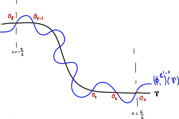
Figure 10. The curves $\gamma$, $(\phi^{h^{\prime}}_{1})^{-1}(\gamma)$ and the points $o_{i}$, $1\leq i\leq l$.

More precisely, $\gamma\cap(\phi_{1}^{h^{\prime}})^{-1}(\gamma)$ consists of an odd number $l$ of intersection points. We denote them by $o_{1},o_{2},\ldots,o_{l}$, as in the picture, and assume that $l\geq 3$; $o_{1}$ is the intersection point with largest real coordinate and $o_{l}$ the intersection point with the smallest real coordinate. The intersection points $o_{i}$ with $i$ odd are called positive (or odd) and the ones with $i$ even are called negative (or even). Notice that $o_{1}$ and $o_{l}$ are bottlenecks - the first along the positive end of $\gamma$ and the second along the negative end.

The definition of $\mathcal{B}_{\gamma,h}$ is now as follows: the objects are $\gamma\times L$ with $L\in\mathcal{L}^{\ast}_{d}(M)$. We abbreviate $\widetilde{L}=\gamma\times L$. To define morphisms and higher operations we first fix all the data needed to define a model for $\mathcal{F}uk^{d}(M)$. Let $\widetilde{L}=\gamma\times L$, $\widetilde{L}^{\prime}=\gamma\times L^{\prime}$ be two objects of $\mathcal{B}_{\gamma,h}$ and denote by $(H_{L,L^{\prime}},J_{L,L^{\prime}})$ the Floer datum that has already been associated to $(L,L^{\prime})$ in $\mathcal{F}uk^{d}(M)$. We put $H_{\widetilde{L},\widetilde{L}^{\prime}}=h^{\prime}\oplus H_{L,L^{\prime}}$ and the time-dependent almost complex structures $J_{\widetilde{L},\widetilde{L}^{\prime}}(t)=i_{h^{\prime}}(t)\oplus J_{L,L^{\prime}}(t)$, $t\in[0,1]$ where

$$i_{h^{\prime}}(t)=(\phi_{t}^{h^{\prime}})_{\ast}i~{}.~{}$$

The Floer datum for $(\widetilde{L},\widetilde{L}^{\prime})$ is defined to be the pair $(H_{\widetilde{L},\widetilde{L}^{\prime}},J_{\widetilde{L},\widetilde{L}^{\prime}})$ and we put

$$\hom_{\mathcal{B}_{\gamma,h}}(\widetilde{L},\widetilde{L}^{\prime})=CF(\widetilde{L},\widetilde{L^{\prime}};H_{\widetilde{L},\widetilde{L}^{\prime}},J_{\widetilde{L},\widetilde{L}^{\prime}})$$

endowed with the standard Floer differential. It is not difficult to verify that this data is regular. Indeed, our choices for $H_{\widetilde{L},\widetilde{L^{\prime}}}$ and $J_{\widetilde{L},\widetilde{L}^{\prime}}$ imply that the relevant Fredholm operators split as a product of the obvious operators in $\mathbb{C}$ and in $M$. Due to the choice of $h^{\prime}$, for each relevant Floer trajectory $u=(u_{1},u_{2})$ where $u_{1}=\pi\circ u$ and $u_{2}=\pi_{2}\circ u$ (with $\pi_{2}:\mathbb{C}\times M\to M$ the projection on the second factor) the respective operators are surjective at $u_{1}$ and $u_{2}$ respectively. The surjectivity at $u_{2}$ is due to the generic choice of $H_{L,L^{\prime}},J_{L,L^{\prime}}$. For the surjectivity at $u_{1}$ we need to separate to two cases according to whether or not $u_{1}$ is constant. If $u_{1}$ is not constant then by automatic regularity for holomorphic curves in $\mathbb{C}$ (see Section 13a in [Sei3] and also [dSRS]) the operator is surjective. If $u_{1}$ is constant then the surjectivity follows from Corollary 4.3.2. Notice, in particular, that the Floer strips that project to a constant in $\mathbb{C}$ equal to one of the points $o_{i}$, be they positive or negative, remain regular as Floer strips in $\mathbb{C}\times M$.

Remark 4.2.1.

It is useful to contrast the regularity indicated above with the situation occurring for curves with boundary conditions along Lagrangians $\widetilde{L}_{1},\ldots,\widetilde{L}_{k+1}$ with $k\geq 2$, that project to one of the constant points $o_{i}$. Of course, these curves do not appear in the definition of the Floer complexes but rather in that of the higher compositions (see below). In this case, the curves that project to positive points $o_{i}$ remain regular but those that project to negative points are not regular in $\mathbb{C}\times M$: indeed, by Corollary 4.3.2, at the negative points the planar operator has a negative index while at the positive points the index is $0$.

To construct the coherent system of categories $\mathcal{B}_{\gamma,h}$ we can now apply the general scheme used to construct the category $\mathcal{F}uk_{cob}^{d}(\mathbb{C}\times M)$ in §3. This involves using quite general perturbations - as in §3.2 - to the left of $o_{1}$ and to the right of $o_{l}$. The techniques in §3.3 and §3.4 apply without change in view of the fact that the points $o_{1}$ and $o_{l}$ are bottlenecks and the same remains true for the invariance results in §3.6.

We use the category $\mathcal{F}uk^{d}_{{cob,1/2}}(\mathbb{C}\times M;i^{\prime},h^{\prime})$ as defined in §4.1 above using a choice of data $i$ that extends the choices just made for $\mathcal{B}_{\gamma,h}$. We thus obtain an obvious full and faithful embedding of $A_{\infty}$-categories:

(45) $$\beta_{\gamma,h}:\mathcal{B}_{\gamma,h}\longrightarrow\mathcal{F}uk^{d}_{{cob,1/2}}(\mathbb{C}\times M;i^{\prime},h^{\prime}).$$

The next step is to define quasi-isomorphisms $\mathcal{B}_{\gamma,h}\to\mathcal{F}uk^{d}(M)$ as well as certain explicit comparison quasi-isomorphisms relating $\mathcal{B}_{\gamma,h_{1}}$ to $\mathcal{B}_{\gamma,h_{2}}$ for different profile functions $h_{1},h_{2}$. The desired inclusion functor will be defined by composing $\beta_{\gamma,h}$ with the inverse of $\mathcal{B}_{\gamma,h}\to\mathcal{F}uk^{d}(M)$. To construct these functors and deduce some of their properties we need a special model for $\mathcal{B}_{\gamma,h}$ associated to particular perturbation data that we describe next.

This perturbation data is only required for the higher compositions $\mu^{k}$, $k\geq 2$, the Floer data is fixed as above. Let $L_{1},\ldots,L_{k+1}\in\mathcal{L}^{\ast}_{d}(M)$, $k\geq 2$ and denote by $(\Theta_{M},\mathbf{J}_{M})$ the perturbation datum of $(L_{1},\ldots,L_{k+1})$ as fixed in $\mathcal{F}uk^{d}(M)$. The perturbation datum $(\Theta,\mathbf{J})$ associated to $(\widetilde{L}_{1},\ldots,\widetilde{L}_{k+1})$ has the following form:

(46) $$\Theta=da_{r}\otimes h^{\prime}+\Theta_{M}+Q\ ,\ \mathbf{J}=\widetilde{i}_{h}\oplus\mathbf{J}_{M}$$

where $\widetilde{i}_{h}=\{\widetilde{i}_{h}(z)\}_{z\in S_{r}}$ is the family of almost complex structures on $\mathbb{R}^{2}$ defined by $\widetilde{i}_{h}=(\phi^{h^{\prime}}_{a_{r}(z)})_{\ast}i$, $z\in S_{r}$. The term $Q$ is a $1$-form $Q\in\Omega^{1}(S_{r},C^{\infty}(\mathbb{C}\times M))$ which is compactly supported in the interior of $S_{r}$ and away from the strip like ends. Moreover $Q$ is required to satisfy the following conditions for all $z\in S_{r}$, $v\in T_{z}S_{r}$:

• The function $Q_{z}(v):\mathbb{C}\times M\to\mathbb{R}$ is of the from $Q_{z}(v)=q_{z}(v)\circ\pi$ with $q_{z}(v):\mathbb{C}\to\mathbb{R}$.

• The function $q_{z}(v)$ is supported in a union $U_{h}$ of small neighborhoods of the points $o_{i}\in\mathbb{C}$ with $i=$ even.

Similarly to what has been done before in the case of $\mathcal{F}uk^{d}(M)$ we define $(\Theta,\mathbf{J})$ so that it extends the Floer data already defined on the strip-like ends of the surfaces $S_{r}$ and so that it is consistent with splitting and gluing in the space $\widehat{\mathcal{S}}^{k+1}$.

Note that if $Q$ is chosen such that for some $z,v$ the function $q_{z}(v)$ does not have a critical point at $o_{i}$, where $i=$ even, then no solution $u$ of (24) can have a constant projection at $o_{i}$. (In contrast, solutions with a constant projection over $o_{i}$ with $i=$ odd definitely exist.)

The class of perturbations described above is sufficient for the regularity of the moduli spaces of perturbed $J$-holomorphic polygons as will be seen in Corollary 4.3.4. Basically, due to our choices, the linearized operator corresponding to equation (24) has at every solution $u$ a horizontal component (corresponding to $\mathbb{R}^{2}$) and a vertical one (corresponding to $M$). The vertical part can be assumed surjective in view of the choices made for $\mathcal{F}uk^{d}(M)$. As for the horizontal part, the argument splits into two cases. The first one is when $\pi\circ u$ is not constant and in that case Lemma 4.3.3 assures surjectivity of the respective operator. The second possible case is that $\pi\circ u$ is constant. As remarked above a (generic) suitable choice of $Q$ assures that $\pi\circ u$ equals to one of the $o_{i}$’s with $i=$ odd. Corollary 4.3.2 then implies surjectivity for the horizontal operator. The actual argument is slightly more complicated as the splitting mentioned above applies for the moduli spaces of polygons with fixed punctures and the moduli spaces we are interested in are associated to polygons with moving punctures - see Corollary 4.3.4.

Notice also that the Floer complex $CF^{\mathcal{B}_{\gamma,h}}(\widetilde{L},\widetilde{L}^{\prime})=\hom_{\mathcal{B}_{\gamma,h}}(\widetilde{L},\widetilde{L}^{\prime})$ splits as a vector space:

$$CF^{\mathcal{B}_{\gamma,h}}(\widetilde{L},\widetilde{L}^{\prime})=\bigoplus_{i=1}^{l}CF(L,L^{\prime}),$$

where $CF(L,L^{\prime})=CF(L,L^{\prime};H_{L,L^{\prime}},J_{L,L^{\prime}})$ is the Floer complex in $\mathcal{F}uk^{d}(M)$. The $i$-th summand at the right-hand side of the above equality corresponds to the point $o_{i}$ and we will sometimes identify it as $CF(L,L^{\prime})^{o_{i}}$. We use the following notation. For $x\in CF(L,L^{\prime})$ and $1\leq i\leq l$ we denote by $x^{(i)}\in CF^{\mathcal{B}_{\gamma,h}}(\widetilde{L},\widetilde{L}^{\prime})$ the element $(0,\ldots,0,x,0\ldots,0)\in CF(L,L^{\prime})^{o_{i}}$ where $x$ is placed at the $i$-the spot. Such an element $(0,\ldots,0,x,0\ldots,0)\in CF(L,L^{\prime})^{o_{i}}\subset CF^{\mathcal{B}_{\gamma,h}}(\widetilde{L},\widetilde{L}^{\prime})$ will be called a morphism of type $o_{i}$. Morphisms of some type $o_{i}$ as before will be called homogeneous. We also denote $CF^{\mathcal{B}_{\gamma,h}}(\widetilde{L},\widetilde{L}^{\prime})^{\leq\alpha}$ the partial sum $\oplus_{i=1}^{\alpha}CF(L,L^{\prime})^{o_{i}}\subset CF^{\mathcal{B}_{\gamma,h}}(\widetilde{L},\widetilde{L}^{\prime})$, $1\leq\alpha\leq l$.

Remark 4.2.2.

It is an easy exercise to describe also the differential $\overline{d}$ of $CF^{\mathcal{B}_{\gamma,h}}(\widetilde{L},\widetilde{L}^{\prime})$. For this let $d:CF(L,L^{\prime})\to CF(L,L^{\prime})$ be the differential of the Floer complex in $\mathcal{F}uk^{d}(M)$. We then have, for $j$ even $\overline{d}x^{(j)}=(dx)^{(j)}$ and for $j$ odd $\overline{d}x^{(j)}=(dx)^{(j)}+x^{(j-1)}-x^{(j+1)}$ (where, by a slight abuse in notation, we put $x^{(j+1)}=0$ if $j=l$ and $x^{(j-1)}=0$ if $j=1$). In particular, the complexes $CF^{\mathcal{B}_{\gamma,h}}(\widetilde{L},\widetilde{L}^{\prime})$ and $CF(L,L^{\prime})$ are quasi-isomorphic.

We will need a strong form of the statement in Remark 4.2.2. For an odd index $1\leq j\leq l$ we define a functor $c_{\gamma,h,j}:\mathcal{B}_{\gamma,h}\to\mathcal{F}uk^{d}(M)$ by putting on objects $c_{\gamma,h,j}(\widetilde{L})=L$, on morphisms $c_{\gamma,h,j}^{1}(x^{(i)})=x$ if $i=j$, $c_{\gamma,h,j}^{1}(x^{(i)})=0$ if $i\not=j$ and $c_{\gamma,h,j}^{r}=0$ for $r\geq 2$.

Proposition 4.2.3.

With the definition above, the $c_{\gamma,h,j}$’s are $A_{\infty}$-functors and are quasi isomorphisms. Moreover, for any two odd $1\leq j,j^{\prime}\leq l$, the functors $c_{\gamma,h,j}$ and $c_{\gamma,h,j^{\prime}}$ are homotopic.

Proof.

In view of Remark 4.2.2, to prove the first part of the claim it is enough to show that $c_{\gamma,h,j}$ is an $A_{\infty}$-functor. For this we start by listing two properties of the higher compositions in $\mathcal{B}_{\gamma,h}$ in the model using the perturbations described above. Denote the compositions in $\mathcal{B}_{\gamma,h}$ by $\overline{\mu}_{k}$ and the compositions in $\mathcal{F}uk^{d}(M)$ by $\mu_{k}$. We assume below $k\geq 2$. Let $z_{i}\in CF(L_{i},L_{i+1})^{o_{j_{i}}}$, $1\leq i\leq k$, and let $u:S_{r}\to\widetilde{M}$ be an index-$0$ solution to (24) with entries $z_{1},\ldots,z_{k}$. Denote by $w\in\widetilde{M}$ the exit (or output) of $u$. We claim that one of the following possibilities occur:

• There exists an odd $s$ such that $j_{1}=\cdots=j_{k}=s$ and $\pi\circ u$ is constant at $o_{s}$. In particular $\overline{\mu}_{k}(z_{1},\ldots,z_{k})=(0,\ldots,0,\mu_{k}(z_{1},\ldots,z_{k}),0,\ldots,0)\in CF(L_{1},L_{k+1})^{o_{s}}$.

• There is an $i$ with $j_{i}=$ even and $w\in CF(L_{1},L_{k+1})^{o_{j_{i}}}$. Moreover, for every $r\neq i$ we have $j_{r}=j_{i}\pm 1$ or $j_{r}=j_{i}$. In particular $\overline{\mu}_{k}(z_{1},\ldots,z_{k})\in CF(L_{1},L_{k+1})^{o_{j_{i}}}$.

The justification of this property is a simple application of two arguments. First, the odd points play a typical “bottleneck” role because our perturbations are such that the curves $u$ transform by the naturality transformation (25) to polygons that project holomorphically onto $\mathbb{C}$ around these points. Moreover, the odd points are “entry” (or input) points from the point of view of the strip-like ends of these projections. This shows that any such curve that has such a point as an “exit” (or output) point has to project to a constant. The second argument is based on Corollary 4.3.4. More specifically, if an even point corresponds to the “exit” then, it is necessary for at least one even point to appear among the entries.

Finally, the fact that $j_{r}=j_{i}\pm 1$ or $j_{r}=j_{i}$ for every $r$ follows from a bottleneck argument similar the ones used previously several times.

The above description of $\overline{\mu}_{k}$ implies the following identity:

$$c^{1}_{\gamma,h,j}(\overline{\mu}_{k}(z_{1},\ldots,z_{k}))=\mu_{k}\bigl{(}c^{1}_{\gamma,h,j}(z_{1}),\ldots,c^{1}_{\gamma,h,j}(z_{k})\bigr{)}.$$

In view of the vanishing of the higher order components of $c_{\gamma,h,j}$ it follows from this identity that $c_{\gamma,h,j}$ is an $A_{\infty}$-functor.

To conclude the proof of the Proposition it remains to show the statement about the homotopy. To simplify the exposition we will now assume that $l=3$. We will show now that $c_{\gamma,h,1}$ and $c_{\gamma,h,3}$ are homotopic as $A_{\infty}$-functors.

Let $k\geq 2$ and let $z_{i}\in CF(L_{i},L_{i+1})^{o_{j_{i}}}$, $1\leq i\leq k$, be so that all $j_{i}\in\{1,3\}$ for every $i$. By inspecting the points i, ii above we see that $\overline{\mu}(z_{1},\ldots,z_{k})=0$ except possibly if all $j_{i}$ are equal to $1$ or if they are all equal to $3$. Moreover, we have

$$\overline{\mu}_{k}(x_{1}^{(1)},\ldots,x_{k}^{(1)})=(\mu_{k}(x_{1},\ldots,x_{k}))^{(1)}\ ,\quad\overline{\mu}_{k}(x_{1}^{(3)},\ldots,x_{k}^{(3)})=(\mu_{k}(x_{1},\ldots,x_{k}))^{(3)}~{}.~{}$$

By Remark 4.2.2 for $k=1$ we have

$$\overline{\mu}_{1}(x^{(1)}+x^{(3)})=(\mu_{1}(x))^{(1)}+(\mu_{1}(x))^{(3)})~{}.~{}$$

We thus define an $A_{\infty}$-functor:

$$e_{\gamma,h}:\mathcal{F}uk^{d}(M)\longrightarrow\mathcal{B}_{\gamma,h}$$

by defining it on objects as $e_{\gamma,h}(L)=\widetilde{L}$, on morphisms $e_{\gamma,h}^{1}(x)=x^{(1)}+x^{(3)}$ and setting the higher components to be null, $e_{\gamma,h}^{k}=0$ for all $k>1$.

This morphism clearly satisfies $c_{\gamma,h,1}\circ e_{\gamma,h}=c_{\gamma,h,3}\circ e_{\gamma,h}=id$. Moreover, $e_{\gamma,h}$ is a quasi-isomorphism and thus invertible up to homotopy. (Note that $e_{\gamma,h}$, in contrast to $c_{\gamma,h,j}$ does not depend on $j$.) Thus, $c_{\gamma,h,1}\simeq c_{\gamma,h,3}$. The argument for $l>3$ is analogous: namely

$$e_{\gamma,h}:\mathcal{F}uk^{d}(M)\to\mathcal{B}_{\gamma,h}$$

has the same definition on objects as in the case $l=3$, its action on morphisms is again null for $k\geq 2$ and $e_{\gamma,h}^{1}(x)=x^{(1)}+x^{(3)}+\ldots+x^{(l)}$. ∎

We now define the inclusion functor

$$\mathcal{I}_{\gamma,h}:\mathcal{F}uk^{d}(M)\longrightarrow\mathcal{F}uk^{d}_{{cob,1/2}}(\mathbb{C}\times M;i^{\prime},h^{\prime})$$

as the composition

(47) $$\mathcal{I}_{\gamma,h}=\beta_{\gamma,h}\circ e_{\gamma,h},$$

where $\beta_{\gamma,h}$ is the functor defined in (45).

Remark 4.2.4.

a. The functor $e_{\gamma,h}$ is a common homotopy inverse for all the projections $c_{\gamma,h,i}$. As all these projections are mutually chain homotopic we will sometimes omit the index $i$ from the notation in $c_{\gamma,h,i}$.

b. If the ends of $\gamma$ have integral $y$-coordinates then $\mathcal{I}_{\gamma,h}$ factors through

$$\mathcal{F}uk^{d}(M)\longrightarrow\mathcal{F}uk^{d}_{cob}(\mathbb{C}\times M;i,h)\stackrel{{\scriptstyle j}}{{\longrightarrow}}\mathcal{F}uk^{d}_{{cob,1/2}}(\mathbb{C}\times M;i^{\prime},h^{\prime}).$$

Proposition 4.2.5.

Up to a quasi-isomorphism (canonical in homology), the functor $\mathcal{I}_{\gamma,h}$ depends only on the horizontal isotopy type of $\gamma$.

Proof.

The proof follows the general method for proving invariance statements as in §3.6. Thus, we first assume that $\gamma$ varies inside a fixed horizontal isotopy type and $h$ changes while keeping fixed the bottlenecks $o_{1}$ and $o_{l}$ and $l$ remains fixed. We then include the different categories $\mathcal{B}_{\gamma,h}$ in the same category $\mathcal{B}^{tot}$. This category comes with a projection $\bar{c}_{1}:\mathcal{B}^{tot}\to\mathcal{F}uk^{d}(M)$ associated to the first intersection point $o_{1}$. This functor $\bar{c}_{1}$ restricts to the projection $c_{\gamma,h,1}$ on each $\mathcal{B}_{\gamma,h}$ and is a quasi-equivalence. Consider now the functors:

$$\mathcal{F}uk^{d}(M)\stackrel{{\scriptstyle e_{\gamma,h}}}{{\longrightarrow}}\mathcal{B}_{\gamma,h}\to\mathcal{B}^{tot}~{}.~{}$$

The composition of $\bar{c}_{1}$ with each one of these functors is the identity. Thus any two such functors are quasi-isomorphic. The category $\mathcal{B}^{tot}$ can be mapped by inclusion into $\mathcal{F}uk_{cob,1/2}^{d,tot}(\mathbb{C}\times M)$ and thus any two functors $\mathcal{I}_{\gamma,h}$ are also quasi-isomorphic by a quasi-isomorphism that is canonical in homology.

The same argument also applies if we vary $h$ by keeping its positive and negative bottlenecks all fixed while allowing the number $l\geq 3$ to change: because the bottlenecks are fixed the corresponding category $\mathcal{B}^{tot}$ remains well defined as well as its inclusion in $\mathcal{F}uk_{cob,1/2}^{d,tot}(\mathbb{C}\times M)$; the projection $c_{1}$ remains also well-defined. The last step is to “move” the bottlenecks. This is achieved combining the argument above with that in §3.6.5. ∎

Remark 4.2.6.

The description of the $A_{\infty}$-structure for the category $\mathcal{B}_{\gamma,h}$ in the proof of Proposition 4.2.3 also allows us to compare explicitly the categories $\mathcal{B}_{\gamma,h}$ and $\mathcal{B}_{\gamma,g}$ where the number of points $o_{i}\in\ C$ for the function $h$ is $l\geq 5$ and the number of points $o^{\prime}_{i}\in\mathbb{C}$ for the function $g$ is $l^{\prime}=l-2$. Indeed, it is easy to define:

$$p^{h}_{g}:\mathcal{B}_{\gamma,h}\to\mathcal{B}_{\gamma,g}$$

which is the identity on objects, it is given on morphisms by $(p^{h}_{g})^{1}(x^{(i)})=x^{(i)}$ if $i\leq l-2$ and $(p^{h}_{g})^{1}(x^{(i)})=0$ if $l-2<i\leq l$ and $(p^{h}_{g})^{k}=0$ for $k\geq 2$. For suitable choices of $g$ and perturbation data it is easy to see that this is an $A_{\infty}$ functor. For this, we pick $g$ so that $(\phi^{g^{\prime}}_{1})^{-1}(\gamma)$ coincides with $(\phi_{1}^{h^{\prime}})^{-1}(\gamma)$ to the right of $o_{l-2}$ and we also fix the perturbation data so that the perturbation data for $\mathcal{B}_{\gamma,h}$ extends that of $\mathcal{B}_{\gamma,g}$. Clearly, $p^{h}_{g}$ is compatible in the obvious sense with the projections $c_{\gamma,h}$ and $c_{\gamma,g}$ as well as with the functors $e_{\gamma,h}$, $e_{\gamma,g}$.

4.3. Index and regularity

The purpose of this subsection is to provide details on the index calculations used above in constructing and analyzing the category $\mathcal{B}_{\gamma,h}$. Recall that we had to calculate the index of the linearized operator associated to equation (24) at a solution $u$ of that equation. We need to calculate the index for two types of solutions $u$. The first is when $u$ has a constant projection to $\mathbb{C}$, and the second one is when the projection is not constant. The main part in this calculation amounts to computing the index of the horizontal part of the operator. We will also address regularity of the solutions.

4.3.1. The case of solutions with constant projection

We will work here with the following slightly more general setting. Let $\gamma\subset\mathbb{R}^{2}$ be a curve as in §4.2. Fix $k\geq 2$. Let $f_{1},\ldots,f_{k+1}:\gamma\longrightarrow\mathbb{R}$ be Morse functions and assume that $p\in\gamma$ is a critical point of all the $f_{i}$’s. Denote by $|p|_{f_{i}}$ the Morse index of $f_{i}$ at $p$. Fix a a punctured disk $S=S_{r}$ for some $r\in\mathcal{R}^{k+1}$ and denote its complex structure by $j$. Denote by $a=a_{r}:S\longrightarrow\mathbb{R}$ the transition function as in §3.1. Let $\{\hat{f}_{z}:\gamma\longrightarrow\mathbb{R}\}_{z\in S}$ be a family of functions, parametrized by $S$, all having $p$ as a critical point and such that on the $i^{\prime}th$ strip-like end of $S$, $f_{z}$ coincides with $f_{i}$ at infinity, i.e. $\hat{f}_{z}=f_{i}$ for every $z\in\epsilon_{i}^{S}(Z^{-}\setminus K^{-})$, $i=1,\ldots,k$ and $\hat{f}_{z}=f_{k+1}$ for every $z\in\epsilon_{i}^{S}(Z^{+}\setminus K^{+})$, where $K^{\pm}$ are compact subsets of the semi-strips. We extend the functions $f_{i}$ and $\hat{f}_{z}$ to functions on $\mathbb{R}^{2}$ by identifying $T^{*}\gamma\cong\mathbb{R}^{2}$ and defining the extension to be constant along each fibers of $T^{*}\gamma$. Denote by $X^{\hat{f}}=\{X^{\hat{f}_{z}}\}_{z\in S}$ the ($S$-dependent) Hamiltonian vector field associated to $\hat{f}$. Set $Z=da\otimes X^{\hat{f}}$ viewed as a $1$-form on $S$ with values in the space of Hamiltonian vector fields on $\mathbb{R}^{2}$. Finally define an $S$-dependent complex structure $\hat{i}=\{\hat{i}_{z}\}_{z\in S}$ on $\mathbb{R}^{2}$ defined by $\hat{i}_{z}=\big{(}\phi_{a(z)}^{\hat{f}_{z}}\big{)}_{*}i$.

We extend the choices above to the case $k=1$ as follows. In that case $S$ can be identified with the strip $\mathbb{R}\times[0,1]$ and we require that $f_{0}=f_{1}$, the family $\hat{f}_{z}$ to be constant and $a(s,t)=t$ for every $(s,t)$.

With the above data fixed, consider the following equation:

(48) $$w:(S,\partial S)\longrightarrow(\mathbb{R}^{2},\gamma),\quad Dw+\hat{i}_{z}(w)\circ Dw\circ j=Z+\hat{i}_{z}(w)\circ Z\circ j.$$

Due to our choices we have $Z_{z}(p)=0$ for every $z\in S$, hence the constant map $w_{0}(z)\equiv p$ is a solution of (48). Denote by $\mathcal{D}_{w_{0}}$ the linearized operator associated to (48) at $w_{0}$.

The following Lemma follows from the theory developed in [Sei4].

Lemma 4.3.1.

The Fredholm index of $\mathcal{D}_{w_{0}}$ is given by

$$\textnormal{ind}(\mathcal{D}_{w_{0}})=|p|_{f_{1}}+\cdots+|p|_{f_{k}}-|p|_{f_{k+1}}-(k-1).$$

Moreover, when the index is $0$ the operator $\mathcal{D}_{w_{0}}$ is surjective, hence the solution $w_{0}$ is regular.

The following is an immediate consequence of the previous lemma.

Corollary 4.3.2.

$\textnormal{ind}(\mathcal{D}_{w_{0}})=0$ in any of the following two cases:

1. $k=1$ and $|p|_{f_{1}}=|p|_{f_{2}}$.

2. $k\geq 2$ and $|p|_{f_{1}}=\cdots=|p|_{f_{k+1}}=1$.

Moreover, in both cases the constant solution $w_{0}$ is regular.

Proof of Lemma 4.3.1.

The proof follows essentially the recipe from Sections 4.5 and 4.6 in [Sei4], with a few minor modifications that we outline below.

We begin with the index formula. Consider the same equation as (48) but with $\hat{i}$ replaced by the standard (constant) complex structure $i$ in the plane $\mathbb{C}$. The constant map $w_{0}$ solves that equation too. The linearized operator $\mathcal{D}^{\prime}_{w_{0}}$ of that equation is homotopic to $\mathcal{D}_{w_{0}}$ through Fredholm operators, hence its index is equals to that of $\mathcal{D}^{\prime}_{w_{0}}$.

The operator $\mathcal{D}^{\prime}_{w_{0}}$ is precisely of the class of operators considered in Section 4e of [Sei4] (see (4.32) and (4.33) in that paper for the precise description of that class). More precisely, the operator $\mathcal{D}^{\prime}_{w_{0}}$ has the following form:

(49) $$\begin{cases}&\mathcal{D}^{\prime}_{w_{0}}(\xi)=\overline{\partial}{\xi}-\Bigl{(}i\circ\textnormal{Re}(\xi)\textnormal{diag}\bigl{(}\hat{f}_{z}^{\prime\prime}(p),0\bigr{)}\otimes da\Bigr{)}^{0,1},\\ &\xi:S\longrightarrow\mathbb{R}^{2},\\ &\xi(z)\in T_{p}\gamma,\;\forall z\in\partial S.\end{cases}$$

Here both sides of the equation are regarded as $1$-forms with values in $\hom_{\mathbb{R}}(\mathbb{C},\mathbb{C})=Mat_{2}(\mathbb{R})$. Also, $\hat{f}_{z}^{\prime\prime}(p)$ stands for the second derivative of the function $\hat{f}_{z}:\gamma\longrightarrow\mathbb{R}$ at the point $p$, where we identify $\gamma$ with $\mathbb{R}$ in the obvious way.

From here on, the index calculation of $\mathcal{D}^{\prime}_{w_{0}}$ follows a topological recipe developed in [Sei4]. Denote by $\bar{S}$ the compactification of $S$ obtained by adding to each strip like end an interval of the type $\epsilon_{i}^{S}(\pm\infty\times[0,1])$. According to [Sei4] we have

$$\textnormal{ind}(\mathcal{D}^{\prime}_{w_{0}})=1+\deg(\hat{\lambda}),$$

where $\hat{\lambda}:\partial\bar{S}\longrightarrow{\mathbb{R}}P^{1}$ is a map defined as $\hat{\lambda}(z)=T_{p}\gamma\in{\mathbb{R}}P^{1}$ for every $z\in\partial S$ and over the intervals at infinity of $\partial\bar{S}$ by using an explicit homotopy class of loops in $\mathbb{R}P^{1}$ starting and ending at $T_{p}\gamma$. This homotopy class is explicitly determined on each end by the sign of $f_{i}^{\prime\prime}(p)$.

A little care is needed when following the procedure from [Sei4], since Seidel’s conventions differ from ours. The essential difference here is that in [Sei4] Seidel parametrizes the strip-like ends in a different way than we do. Namely, the “input” (or “entry”) ends $i=1,\ldots,k$ are parametrized in Seidel by $[0,\infty)\times[0,1]$ whereas we parametrize them by $(-\infty,0]\times[0,1]$. Similarly, the “output” (or “exit”) end is parametrized in Seidel by $(-\infty,0]\times[0,1]$ and we parametrize it by $[1,\infty)\times[0,1]$. The outcome is that in order to calculate the map $\bar{\lambda}$ using the conventions of Seidel we need to replace $f_{i}^{\prime\prime}(p)$ by $-f_{i}^{\prime\prime}(p)$ everywhere. Apart from that a straightforward substitution in the method from [Sei4] yields the desired index formula.

We now turn to regularity, under the assumption that the index is $0$. Here it is convenient to apply the naturality transformation, namely define $v:S\longrightarrow\mathbb{R}^{2}$ by the transformation $w(z)=\phi_{a(z)}^{\hat{f}_{z}}(v(z))$. Then the equation (48) is transformed to the following equation with moving boundary conditions:

(50) $$\begin{cases}&Dv+i\circ Dv_{z}\circ j=0,\\ &v:S\longrightarrow\mathbb{R}^{2},\\ &v(z)\in\bigl{(}\phi_{a(z)}^{\hat{f}_{z}}\bigr{)}^{-1}(\gamma),\;\forall z\in\partial S.\end{cases}$$

Note that the constant solution $w_{0}$ is sent by this transformation to the constant solution $v_{0}\equiv p$ of equation (50). The linearization $\mathcal{D}^{\prime\prime}_{v_{0}}$ of (50) at $v_{0}$ now looks as follows:

(51) $$\begin{cases}&\mathcal{D}^{\prime\prime}_{v_{0}}(\xi)=\overline{\partial}{\xi}\\ &\xi:S\longrightarrow\mathbb{R}^{2},\\ &\xi(z)\in D\bigl{(}\phi_{a(z)}^{\hat{f}_{z}}\bigr{)}^{-1}(T_{p}\gamma),\;\forall z\in\partial S.\end{cases}$$

This operator still falls in the class of operators considered in [Sei4] (see Section 4.5 in that paper). The index can now be independently (of the previous calculation) calculated via an analogous procedure: $\textnormal{ind}(\mathcal{D}^{\prime\prime}_{v_{0}})=1+\deg(\hat{\lambda})$, where this time the map $\hat{\lambda}$ takes into account also the moving boundary conditions $D\bigl{(}\phi_{a(z)}^{\hat{f}_{z}}\bigr{)}^{-1}(T_{p}\gamma)$, $z\in\partial S$. Since the total index is assumed to be $0$ we have $\deg(\hat{\lambda})=-1$. By Proposition 4.1 in [Sei4] this implies that $\mathcal{D}^{\prime\prime}_{v_{0}}$ is injective. As the index is $0$ it must also be surjective. ∎

4.3.2. The case of solutions with non-constant projection

Here we consider a very similar setting to the one in §4.3.1 with the following difference. The functions $f_{1},\ldots,f_{k+1}:\gamma\longrightarrow\mathbb{R}$ are assumed to be Morse but possibly with different critical points. The family $\hat{f}$ is only assumed to coincide with the $f_{i}$’s on the ends at infinity. The term $Z$ in equation (48) is allowed now to have following more general form:

$$Z=da\otimes X^{\hat{f}}+X^{q},$$

where $q$ is a $1$-form on $S$ with values in $C^{\infty}(\mathbb{R}^{2})$ whose support (as a form on $S$) is compact and lies inside the interior of $S$. The main example we have in mind is when the $f_{i}$’s, as well as the $\hat{f}_{z}$’s all coincide with one extended profile function $h^{\prime}$, and the form $q$ is as defined on page 46 after equation (46).

Let $w:(S,\partial S)\longrightarrow(\mathbb{R}^{2},\gamma)$ be a solution of equation (48), where $Z$ is now assumed to be of the form just discussed. It is easy to see that along each strip-like end $w$ converges to a critical point of the corresponding $f_{i}$. Denote by $p_{1},\ldots,p_{k}\in\gamma$ the critical points corresponding to the input ends and by $p_{k+1}$ the one corresponding to the output. We write $|p_{i}|_{f_{i}}$ for the Morse index of $f_{i}$ at $p_{i}$. We continue to denote the linearized operator of (48) at $w$ by $\mathcal{D}_{w}$. Let $r\in\mathcal{R}^{k+1}$ be the point parametrizing the punctured disk $S$ (so that $S=S_{r}$) and denote by $\overline{\mathcal{D}}_{r,w}$ the extended linearized operator, that takes into account “moving” punctures. The following Lemma follows too from the methods of [Sei4].

Lemma 4.3.3.

Let $w$ be a non-constant solution of equation (48). Then the operator $\overline{\mathcal{D}}_{r,w}$ is surjective and its index is given by:

$${\textnormal{ind}(\overline{\mathcal{D}}_{r,w})}=|p_{1}|_{f_{1}}+\cdots+|p_{k}|_{f_{k}}-|p_{k+1}|_{f_{k+1}}-{1}.$$

Proof.

The proof is very similar to the proof of Lemma 4.3.1, following the theory from Sections 4.5 and 4.6 of [Sei4].

By applying a suitable symplectomorphism of $\mathbb{R}^{2}$ we may assume without loss of generality that the curve $\gamma$ is entirely horizontal. The map $\hat{\lambda}$ mentioned in the proof of Lemma 4.3.1 then becomes constant over $\partial S$ (since $\hat{\lambda}(z)=T_{w(z)}\gamma$   $\forall z\in\partial S$). Thus the only contribution of $\hat{\lambda}$ to the index of $\mathcal{D}_{w}$ comes from the ends of $S$. But the calculation over each end coincides with that done for the proof of Lemma 4.3.1.

The index of $\overline{\mathcal{D}}_{r,w}$ is bigger by $k-2$ compared to that of $\mathcal{D}_{w}$ and, finally, the surjectivity of $\overline{\mathcal{D}}_{r,w}$ follows from the theory developed in Section 13a of [Sei3]. ∎

We now examine the situation for polygons in $\mathbb{R}^{2}\times M$. Let $L_{1},\ldots,L_{k+1}\in\mathcal{L}^{*}_{d}(M)$ and $\widetilde{L}_{1},\ldots,\widetilde{L}_{k+1}$ as in §4.2. Let $\gamma_{i}\in CF(\widetilde{L}_{i},\widetilde{L}_{i+1};H_{\widetilde{L}_{i},\widetilde{L}_{i+1}},J_{\widetilde{L}_{i},\widetilde{L}_{i+1}})$, $i=1,\ldots,k$, and $\gamma_{k+1}\in CF(\widetilde{L}_{1},\widetilde{L}_{k+1};H_{\widetilde{L}_{1},\widetilde{L}_{k+1}},J_{\widetilde{L}_{1},\widetilde{L}_{k+1}})$ be generators.

Corollary 4.3.4.

For a generic choice of perturbation data $\mathscr{D}_{M}=(\Theta_{M},\mathbf{J}_{M})$ in $M$, the moduli spaces $\mathcal{M}(\gamma_{1},\ldots,\gamma_{k},\gamma_{k+1};\mathscr{D}_{\mathbb{R}^{2}\times M})$ of polygons in $\mathbb{R}^{2}\times M$, defined using the perturbation data $\mathscr{D}_{\mathbb{R}^{2}\times M}=(\Theta,\mathbf{J})$ as in (46), are regular. Moreover, for $k\geq 2$, if all the points $\pi(\gamma_{1}),\ldots,\pi(\gamma_{k})$ are of odd type and the space $\mathcal{M}(\gamma_{1},\ldots,\gamma_{k},\gamma_{k+1};\mathscr{D}_{\mathbb{R}^{2}\times M})$ has a $0$-dimensional component which is not empty, then $\pi(\gamma_{k+1})$ is also of odd type.

Proof.

Consider the “horizontal” moduli spaces, as in Lemma 4.3.3, that we will denote for brevity by $\mathcal{M}_{k+1}(\mathbb{R}^{2};\mathscr{D}_{\mathbb{R}^{2}})$. Consider also the “vertical” moduli spaces $\mathcal{M}_{k+1}(M;\mathscr{D}_{M})$ that are considered in the construction of the Fukaya category of $M$, as in §2.5, and are associated to the system of perturbations $\mathscr{D}_{M}$ and strip-like ends, compatible with gluing. Here $k$ is the number of inputs of the respective polygons. In both cases we will consider moduli spaces of arbitrary dimensions. The horizontal ones are regular by Lemma 4.3.3. Standard arguments imply that, for a generic choice of perturbations $\mathscr{D}_{M}$, the moduli spaces of the second type are also regular. We have two obvious projection maps: $p_{1}:\mathcal{M}_{k+1}(\mathbb{R}^{2};\mathscr{D}_{\mathbb{R}^{2}})\to\mathcal{R}^{k+1}$ and $p_{2}^{\mathscr{D}_{M}}:\mathcal{M}_{k+1}(M;\mathscr{D}_{M})\to\mathcal{R}^{k+1}$. The split nature of the perturbation datum in (46) implies that the moduli space that assembles the curves in $\mathcal{M}(\gamma_{1},\ldots,\gamma_{k},\gamma_{k+1};\mathscr{D}_{\mathbb{R}^{2}\times M})$ is given by the fiber product $\mathcal{M}_{k+1}(\mathbb{R}^{2};\mathscr{D}_{\mathbb{R}^{2}})\times_{\mathcal{R}^{k+1}}\mathcal{M}_{k+1}(M;\mathscr{D}_{M})$ over the two projections $p_{1}$ and $p_{2}^{\mathscr{D}_{M}}$. By standard arguments, a further generic choice of perturbations $\mathscr{D}_{M}$ is sufficient to make the projection $p_{2}^{\mathscr{D}_{M}}$ transverse to $p_{1}$. Consequently, for a generic choice of perturbations $\mathscr{D}_{M}$ the moduli space $\mathcal{M}(\gamma_{1},\ldots,\gamma_{k},\gamma_{k+1};\mathscr{D}_{\mathbb{R}^{2}\times M})$ is regular. Its dimension is given by the sum of the dimensions of the “horizontal” and “vertical” spaces $-(k-2)$.

Assume by contradiction that, $k\geq 2$ and $\mathcal{M}(\gamma_{1},\ldots,\gamma_{k},\gamma_{k+1};\mathscr{D}_{\mathbb{R}^{2}\times M})$ has a component of dimension $0$ such that $\pi(\gamma_{1}),\ldots,\pi(\gamma_{k})$ are all of odd type but $\pi(\gamma_{k+1})$ is of even type. Let $(r,u)$ be an element of the $0$-dimensional component of $\mathcal{M}(\gamma_{1},\ldots,\gamma_{k},\gamma_{k+1};\mathscr{D}_{\mathbb{R}^{2}\times M})$. The total index of the extended operator $\overline{\mathcal{D}}_{r,u}$ is

$$0=ind(\overline{\mathcal{D}}_{r,u})=ind^{\mathrm{hor}}(r,u)+ind^{\mathrm{ver}}(r,u)-(k-2),$$

where $ind^{\mathrm{hor}}$ and $ind^{\mathrm{ver}}$ are the obvious horizontal and vertical indices. They coincide with the indices of the projections of $u$, respectively, to $\mathbb{R}^{2}$ and to $M$. By Lemma 4.3.3, the horizontal index is $ind^{\mathrm{hor}}(r,u)=k-1$ which implies that $ind^{\mathrm{ver}}(r,u)=-1$ and leads to a contradiction, thus ending the proof. ∎

Remark 4.3.5.

In the earlier published version of this paper this subsection contained a mistake confusing between the moduli spaces with fixed punctures and those with “moving punctures”. This led to an error in the statement of the original version of Lemma 4.3.3 as well as to a wrong version of Corollary 4.3.4. The above Lemma 4.3.3 and Corollary 4.3.4 should therefore replace the corresponding ones in the previous version of the paper. The only impact of this correction on the rest of the paper has to do with the proof of Proposition 4.2.3. Namely, the possibility at point ii in the proof of Proposition 4.2.3 needs to allow for curves with multiple even entries - as indicated in the present version - and not just with a single even entry, as claimed in the earlier version. However, the potential existence of these more general curves is immaterial to any of the other arguments, formulas and results in the paper.

The errors in the earlier version of this subsection were discovered by Emily Campling. We are grateful to her for pointing them out to us.

4.4. The exact triangles

4.4.1. $A_{\infty}$-modules associated to a cobordism

Let $V$ be a Lagrangian cobordism $V\in\mathcal{CL}_{d}(M)$, $\gamma\subset\mathbb{C}$ a curve and $h$ a profile function, as in §4.2. (See Figure 10.) We assume that $\#(\gamma\cap(\phi_{1}^{h^{\prime}})^{-1}(\gamma))=l$ where $h^{\prime}$ is the extended profile function associated to $h$.

Consider the Yoneda embedding

$$\mathcal{Y}:\mathcal{F}uk^{d}_{cob,1/2}(\mathbb{C}\times M;i^{\prime},h^{\prime})\to\textnormal{\sl fun}(\mathcal{F}uk^{d}_{cob,1/2}(\mathbb{C}\times M;i^{\prime},h^{\prime}),Ch^{\textnormal{opp}})$$

and the composition of functors

(52) $$\mathcal{Y}(V)\circ\mathcal{I}_{\gamma,h}\ :\ \mathcal{F}uk^{d}(M)\stackrel{{\scriptstyle\mathcal{I}_{\gamma,h}}}{{\longrightarrow}}\mathcal{F}uk^{d}_{cob,1/2}(\mathbb{C}\times M;i^{\prime},h^{\prime})\stackrel{{\scriptstyle\mathcal{Y}(V)}}{{\longrightarrow}}Ch^{\textnormal{opp}}$$

where $\mathcal{I}_{\gamma,h}$ is the inclusion functor from equation (47). As recalled in §A.3.2, $Ch^{\textnormal{opp}}$- valued functors defined on an $A_{\infty}$-category $\mathcal{A}$ are naturally identified with modules over $\mathcal{A}$. Let $\mathcal{M}_{V,\gamma,h}$ be the $\mathcal{F}uk^{d}(M)$-module that corresponds to $\mathcal{Y}(V)\circ\mathcal{I}_{\gamma,h}$. Explicitly, this module is given by $\mathcal{M}_{V,\gamma,h}(N)=CF^{cob}(\gamma\times N,V)$ for all $N\in\mathcal{L}^{\ast}_{d}$ and

$$\mu^{\mathcal{M}_{V,\gamma,h}}:CF(N_{1},N_{2})\otimes\ldots CF(N_{k-1},N_{k})\otimes CF^{cob}(\gamma\times N_{k},V)\to CF^{cob}(\gamma\times N_{1},V)$$

is given by $\mu^{\mathcal{M}_{V,\gamma,h}}(a_{1},\ldots,a_{k-1},b)=\mu^{cob}(e^{1}_{\gamma,h}(a_{1}),\ldots,e^{1}_{\gamma,h}(a_{k-1}),b)$.

Recall from (47) that $\mathcal{I}_{\gamma,h}=\beta_{\gamma,h}\circ e_{\gamma,h}$. Thus we also have a functor

$$\mathcal{Y}(V)\circ\beta_{\gamma,h}\ :\ \mathcal{B}_{\gamma,h}\to\mathcal{F}uk^{d}_{cob,1/2}(\mathbb{C}\times M;i^{\prime},h^{\prime})\to Ch^{\textnormal{opp}}$$

with a corresponding $\mathcal{B}_{\gamma,h}$-module $\overline{\mathcal{M}}_{V,\gamma,h}$ and we have

$$\mathcal{M}_{V,\gamma,h}=e_{\gamma,h}^{\ast}(\overline{\mathcal{M}}_{V,\gamma,h})~{}.~{}$$

In view of Remark 4.2.4 and of the invariance properties of $\mathcal{F}uk_{cob}^{d}(\mathbb{C}\times M)$, it follows that the quasi-isomorphism type of the module $\mathcal{M}_{V,\gamma,h}$ only depends on the horizontal isotopy types of $\gamma$ and $V$. The relevant quasi-isomorphism can be constructed explicitly for $\gamma,h$ fixed and $V$ horizontally isotopic to $V^{\prime}$ via an isotopy $\Phi$. The result is a quasi-isomorphism

$$\Phi^{V}_{V^{\prime}}:\overline{\mathcal{M}}_{V,\gamma,h}\to\overline{\mathcal{M}}_{V^{\prime},\gamma,h}$$

that is constructed by counting $J$-holomorphic polygons with boundary conditions along $\gamma\times N_{1},\ldots,\gamma\times N_{k}$ and with the $k+1$ side satisfying a moving boundary condition along $\Phi_{t}(V)$.

4.4.2. Exact triangles associated to a cobordism

In this subsection we use the theory developed above to construct the exact triangles described in the introduction in equation (4). Even if we are interested in these triangles at the derived level it is important to note that the actual construction needs to be performed before derivation and thus it is by necessity very explicit.

Let $V:L\leadsto(L_{1},\ldots,L_{m})$ be a Lagrangian cobordism in $\mathcal{CL}_{d}(\mathbb{C}\times M)$. Consider a sequence of plane curves $\gamma_{1},\ldots,\gamma_{m}\subset\mathbb{C}$ as in Figure 11. We also choose profile functions $h_{i}$ and associated extended profile functions $h^{\prime}_{i}$ so that $(\phi_{1}^{h^{\prime}_{i}})^{-1}(\gamma_{i})$ are as in Figure 11 (where it is drawn for $m=4$).

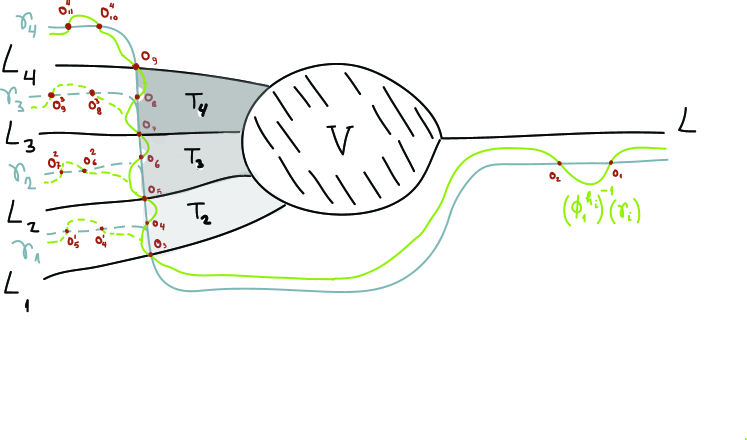
Figure 11. The cobordism $V$, the curves $\gamma_{j}$, and $(\phi_{1}^{h^{\prime}_{j}})^{-1}(\gamma_{j})$, the points $o^{j}_{i}$ and the regions $T_{i}$.

More precisely, our choices are as follows. As before, we identify $\mathbb{C}\cong\mathbb{R}^{2}$ in the standard way. All the curves $\gamma_{i}$ will be of the (general) shape depicted in Figure 10 but with different heights for their ends. We first pick $\gamma_{m}$ so that the height of its negative end is $m+\frac{1}{2}$ and the height of its positive end is $\frac{3}{2}$. Additionally we require that $\gamma_{m}$ coincides with a vertical line of real coordinate $\eta_{\gamma_{m}}<0$ in between the intersections with the $L_{1}$ end of $V$ and the intersection with the $L_{m}$ end. We now pick $h_{m}$ so there are $2m+3$ intersection points $\{o^{m}_{i}\}=(\phi_{1}^{h^{\prime}_{m}})^{-1}(\gamma_{m})\cap\gamma_{m}$ that are so that $o^{m}_{1}$ is a bottleneck and $o^{m}_{1}=(\frac{5}{2},\frac{1}{2})$. Similarly, we require that $o^{m}_{2m+3}$ is a bottleneck and $o^{m}_{2m+3}=(-\frac{3}{2},m+\frac{1}{2})$. The positive intersections satisfy $o^{m}_{2i+1}=\gamma_{m}\cap(i\textnormal{'th negative end of }V)$, $1\leq i\leq m$. Further, we assume that the negative intersections $o^{m}_{2i}$ are of height $i-\frac{1}{2}$, $1\leq i\leq m+1$. The choice of the curves $\gamma_{j}$ for $j<m$ is such that this curve has essentially the same shape as $\gamma_{m}$, it coincides with $\gamma_{m}$ below the height $i+\frac{1}{4}$ and its negative end is of height $i+\frac{1}{2}$. Moreover, $h^{\prime}_{j}$ is such that $(\phi_{1}^{h^{\prime}_{j}})^{-1}(\gamma_{j})$ coincides with $(\phi_{1}^{h^{\prime}_{m}})^{-1}(\gamma_{m})$ for all points $(x,y)\in\mathbb{C}$ with $y\leq j+\frac{1}{4}$. This means, in particular, that we have $o^{j}_{i}=o^{m}_{i}$ for all $1\leq i\leq 2j+1$. Finally, $o^{j}_{2j+3}$ is a bottleneck with $o^{j}_{2j+3}=(-\frac{3}{2},j+\frac{1}{2})$ and $o^{j}_{2j+2}$ is of height $j+\frac{1}{2}$.

Next we pick the Floer and perturbation data required to define the categories $\mathcal{B}_{j}=\mathcal{B}_{\gamma_{j},h_{j}}$, as in the construction of the inclusion functors in §4.2. Additionally, we require that the data for $\mathcal{B}_{\gamma_{j+1},h_{j+1}}$ extends in the obvious sense the data for $\mathcal{B}_{\gamma_{j},h_{j}}$. We now define a sequence of auxiliary $A_{\infty}$-categories $\mathcal{B}^{\prime}_{j}$ for each $1\leq j\leq m$. These have the same objects as $\mathcal{B}_{j}$ and their morphisms are defined algebraically as the following quotients:

(53) $$\hom^{\mathcal{B}^{\prime}_{j}}(\widetilde{N}^{\prime},\widetilde{N}^{\prime\prime})=\hom^{\mathcal{B}_{j}}(\widetilde{N}^{\prime},\widetilde{N}^{\prime\prime})/\langle o^{j}_{2j+2},o^{j}_{2j+3}\rangle,$$

where the “denominator” in the quotient stands for the subspace generated by the intersection points that project to $o^{j}_{2j+2}$ and $o^{j}_{2j+3}$. There is an obvious projection

$$p_{j}:\mathcal{B}_{j}\to\mathcal{B}^{\prime}_{j}$$

given by a formula analogous to that of $p^{h}_{g}$ from Remark 4.2.6. The description of the higher compositions in the proof of Propositions 4.2.3 shows that $\mathcal{B}^{\prime}_{j}$ so defined and endowed with the obvious compositions inherited from $\mathcal{B}_{j}$ is an $A_{\infty}$-category and that $p_{j}$ is an $A_{\infty}$-functor. Notice also that there is a further, similar, projection

$$q_{j}:\mathcal{B}^{\prime}_{j}\to\mathcal{B}^{\prime}_{j-1}$$

that sends to $0$ the morphisms of type $o^{j}_{i}$ with $i=2j,2j+1$. Again this is well defined due to the description of the higher compositions in $\mathcal{B}_{\gamma,h}$, the fact that the points $o^{j}_{i}$ coincide with $o^{j-1}_{i}$ for $1\leq i\leq 2j-1$ together with our choices of Floer and perturbation data. Recall also the map $e_{\gamma,h}$ from (47) and let $e_{j}=e_{\gamma_{j},h_{j}}:\mathcal{F}uk^{d}(M)\to\mathcal{B}_{j}$ and $e^{\prime}_{j}=p_{j}\circ e_{j}$. It is immediate to see that:

(54) $$e^{\prime}_{j-1}=q_{j}\circ e^{\prime}_{j}~{}.~{}$$

We recall also the projection functors $c_{\gamma,h,i}$ from Propositions 4.2.3. Specifically in our case, the $c_{\gamma_{j},h_{j},i}:\mathcal{B}_{j}\to\mathcal{F}uk^{d}(M)$ is the projection on the morphisms of type $o^{j}_{i}$. Clearly, it descends to $c^{\prime}_{\gamma_{j},h_{j},i}:\mathcal{B}^{\prime}_{j}\to\mathcal{F}uk^{d}(M)$ as long as $i\leq 2j+1$. For each $j$, we will mainly be interested in the last of these functors which we denote for brevity by $\sigma_{j}=c^{\prime}_{\gamma_{j},h_{j},2j+1}$.

The fundamental result here concerns the structure of the modules $\overline{\mathcal{M}}_{j}=\overline{\mathcal{M}}_{V,\gamma_{j},h_{j}}$.

Proposition 4.4.1.

For all $1\leq j\leq m$, there are $\mathcal{B}^{\prime}_{j}$-modules $\mathcal{M}^{\prime}_{j}$ with the following properties:

• $p^{\ast}_{j}(\mathcal{M}^{\prime}_{j})=\overline{\mathcal{M}}_{j}$.

• $\mathcal{M}^{\prime}_{1}=\sigma_{1}^{\ast}\,\mathcal{Y}(L_{1})$

• For $j\geq 2$, there is a $\mathcal{B}^{\prime}_{j}$-module morphism

  $$\phi_{j}:\sigma_{j}^{\ast}\,\mathcal{Y}(L_{j})\longrightarrow q^{\ast}_{j}\,\mathcal{M}^{\prime}_{j-1}$$

  so that $\mathcal{M}^{\prime}_{j}=\textnormal{Cone}(\phi_{j})~{}.~{}$

Here $\mathcal{Y}(L_{j})$ is the $\mathcal{F}uk^{d}(M)$-module associated to $L_{j}$ by the Yoneda embedding and $\textnormal{Cone}(\phi_{j})$ is the cone over the module morphism $\phi_{j}$ (see §A.5).

Proof.

Fix $j\in\{1,\ldots,m\}$. The proof is based on the properties of the compositions $\mu^{\overline{\mathcal{M}}_{j}}$.

We will use the notation in §4.2.3 that we first adapt to the module $\overline{\mathcal{M}}_{j}$. For each $N\in\mathcal{L}^{\ast}_{d}$, we notice that $\overline{\mathcal{M}}_{j}(N)=CF^{cob}(\gamma_{j}\times N,V)$ splits as a vector space as

(55) $$\overline{\mathcal{M}}_{j}(N)=\bigoplus_{i=1}^{j}CF(N,L_{i})~{}.~{}$$

We will denote the summand $CF(N,L_{i})$ in this decomposition by $CF^{\overline{\mathcal{M}}_{j}}(N,L_{i})$ and we denote the partial sum $\oplus_{i=1}^{s}CF(N,L_{i})$ by $\overline{\mathcal{M}}_{j}(N)^{\leq s}$. The generators of $CF^{\overline{\mathcal{M}}_{j}}(N,L_{i})$ project to the point $o^{j}_{2i+1}\in\mathbb{C}$ and thus we will refer to the elements in $CF^{\overline{\mathcal{M}}_{j}}(N,L_{i})$ as the elements of $\overline{\mathcal{M}}_{j}(N)$ of type $o^{j}_{2i+1}$.

Fix $N_{1},\ldots,N_{k}\in\mathcal{L}^{\ast}_{d}$ and

$$z_{i}\in CF(N_{i},N_{i+1})^{o_{l_{i}}}\subset CF^{\mathcal{B}_{\gamma_{j},h_{j}}}(\widetilde{N}_{i},\widetilde{N}_{i+1})\ ,\ b\in CF^{\overline{\mathcal{M}}_{j}}(N_{k},L_{s})\subset CF^{cob}(\widetilde{N}_{k},V)$$

where $1\leq l_{i}\leq 2j+3$, $1\leq s\leq j$ and $\widetilde{N}_{1}=\gamma_{j}\times N_{1},\ldots,\widetilde{N}_{k}=\gamma_{j}\times N_{k}$.

Lemma 4.4.2.

With the notation above we have:

• $\mu^{\overline{\mathcal{M}}_{j}}(z_{1},\ldots,z_{k-1},b)\in\overline{\mathcal{M}}_{j}(N)^{\leq s}~{}.~{}$

• If $\mu^{\overline{\mathcal{M}}_{j}}(z_{1},\ldots,z_{k-1},b)\not=0$, then $l_{i}\leq 2s+1$ for all $i=1,\ldots,k-1$.

Proof of Lemma 4.4.2.

Consider a perturbed $J$-holomorphic polygon $u:S_{r}\to\mathbb{C}\times M$ that contributes to $\mu^{\overline{\mathcal{M}}_{j}}_{k}$. Thus $u$ satisfies the equation (46) with boundary conditions along $\widetilde{N}_{1},\ldots,\widetilde{N}_{k},V$. It has entries $z_{1},\ldots,z_{k-1},b$ and denote its exit by $c\in CF^{\overline{\mathcal{M}}_{j}}(N_{1},L_{t})$, where $1\leq t\leq j$.

To simplify the argument, we will choose the profile functions $h_{j}$ and the perturbation data for all tuples of the type $\gamma_{j}\times N_{1},\ldots,\gamma_{j}\times N_{k},V$ to be so that the Hamiltonian flow $\phi_{t}^{h_{j}^{\prime}}$ of the extended profile functions $h^{\prime}_{j}$ keep $V$ invariant. Moreover, choose the $\Theta_{0}$-part of the perturbation data $(\Theta,\mathbf{J})$ to be so that the Hamiltonian functions associated to $\Theta_{0}$ all vanish near $V$, similar to the choices made for the category $\mathcal{B}_{\gamma,h}$ in §4.2. This is all possible since $\gamma_{j}$ intersects $\pi(V)$ transversly. See Figure 11. Note also that the negative intersection points between $\gamma_{j}$ and $(\phi_{1}^{h_{j}^{\prime}})^{-1}(\gamma_{j})$ are away from $\pi(V)$.

We again denote by $v$ the polygon obtained from $u$ by the naturality equation (25) and we let $v^{\prime}=\pi\circ v$ be its planar projection. We now notice that $v^{\prime}$ is holomorphic in a neighborhood of $\partial S_{r}$. Moreover, $v^{\prime}$ is also holomorphic at all points $z\in S_{r}$ so that $v^{\prime}(z)$ belongs to the complement of the region $K_{j}\subset\mathbb{C}$, where

$$K_{j}=U_{h_{j}}\ \cup\ \bigcup_{\tau=0}^{1}(\phi_{\tau}^{h^{\prime}_{j}})^{-1}(\gamma_{j})\ \cup\ \pi(V).$$

Here $U_{h_{j}}$ stands for the union of small neighborhoods of the negative points $o^{j}_{2i}$ used in the construction of $\mathcal{B}_{\gamma_{j},h_{j}}$, see §4.2. By Proposition 3.3.1, as soon as a component of $\mathbb{C}\setminus K_{j}$ intersects the image of $v^{\prime}$, it is completely contained in it. In particular, $v^{\prime}(S_{r})$ can not intersect any unbounded such component. To continue, it is useful to identify the bounded connected components of $\mathbb{C}\backslash K_{j}$: we denote by $T_{i}$, $i=2,\ldots,j$, the (bounded) connected component whose closure contains the points $o^{j}_{2i-1}$ and $o^{j}_{2i+1}$; there are in all $j-1$ such components, see again Figure 11. An important property of these components is that if $T_{i}\subset v^{\prime}(S_{r})$ then one of the following four possibilities occurs:

• there is some point $z\in S_{r}$ so that $v^{\prime}(z)=o^{j}_{2i+1}$.

• $o^{j}_{2i+1}$ is the projection of one of the $z_{q}$’s and the strip-like end corresponding to this $z_{q}$ has an image that covers the “great angle” between $\gamma_{j}$ and $(\phi_{1}^{h^{\prime}_{j}})^{-1}(\gamma_{j})$, see Figure 12.

• $\pi(c)=o^{j}_{2i+1}$.

• $\pi(b)=o^{j}_{2i+1}$.

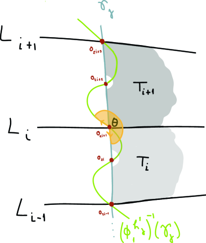
Figure 12. The “great angle” between $\gamma_{j}$ and $(\phi_{1}^{h^{\prime}_{j}})^{-1}(\gamma_{j})$.

Given that $c$ is an exit point for $u$, we notice that if one of 1, 2, or 3 takes place, then the connected region of $\mathbb{C}\backslash K_{j}$ above $T_{i}$ is also contained in $v^{\prime}(S_{r})$. We now claim that if possibility 4 does not occur then:

(56) $$\mathrm{if\ }T_{i}\subset v^{\prime}(S_{r})\;\;\textnormal{then}\;\;i+1\leq s~{}.~{}$$

In other words, if $v^{\prime}$ intersects $T_{i}$, then the point $o^{j}_{2s+1}$, which is the projection of the entry $b$, is “above” $T_{i}$. To see this assume $s\leq i$. Then the argument above shows that case 4 does not apply and thus the region above $T_{i}$ is also in $v^{\prime}(S_{r})$. In case $i=j-1$ we have already arrived to a contradiction as the region above $T_{j-1}$ is not bounded. If $i<j-1$ this region is $T_{i+1}$ and by repeating the same argument now applied to $T_{i+1}$ we deduce that the region above $T_{i+1}$ is again in $v^{\prime}(S_{r})$. Recursively, we arrive to a contradiction. The properties 1,2,3,4 also apply to the point $o^{j}_{2i+1}$ and an argument similar to the above, but using the fact that $b$ is an entry point, shows that

(57) $$\textnormal{if}\;\;T_{i}\subset v^{\prime}(S_{r})\;\;\textnormal{then}\;\;t\leq i.$$

If $v^{\prime}$ is not constant, then $T_{s-1}\subset v^{\prime}(S_{r})$. Thus, putting together (56) and (57), we obtain $t<s$ which shows the point a in the statement of our lemma. Notice that

(58) $$\textnormal{if}\;\;t=s\;\;\textnormal{then}\;\;v^{\prime}\;\;\textnormal{is constant}~{}.~{}$$

Indeed, if $v^{\prime}$ is not constant, then $v^{\prime}(S_{r})$ has to contain $T_{s-1}$ and this implies by (56) and (57) that $t<s$.

To show the point b we clearly may assume that the curve $v^{\prime}$ is not constant. Suppose that there is some $q\in{1,\ldots,k-1}$ so that $o_{j_{q}}>2s+1$. Given that $t<s$ and using that the points $z_{i}$ are entries, it follows that one of the following two possibilities takes place:

• there is a point $z$ belonging to one of the first $k-1$ edges of $S_{r}$ (these are the edges corresponding to the boundary conditions $\widetilde{N}_{1},\ldots,\widetilde{N}_{k-1}$) so that $v^{\prime}(z)=o^{j}_{2s+1}$.

• there is some $q^{\prime}$ so that $\pi(z_{q^{\prime}})=o^{j}_{2s+1}$ and the image by $v^{\prime}$ of the strip-like end associated to $z_{q^{\prime}}$ covers the “great angle” between $\gamma_{j}$ and $(\phi_{1}^{h_{j}})^{-1}(\gamma_{j})$ at $o^{j}_{2s+1}$.

Both 1’ and 2’ show that the connected region of $\mathbb{C}\backslash K_{j}$ above $o^{j}_{2s+1}$ intersects $v^{\prime}(S_{r})$ which contradicts (56) and ends the proof of the lemma. ∎

We now return to the proof of Proposition 4.4.1. The first step is to define the $\mathcal{B}^{\prime}_{j}$-modules $\mathcal{M}^{\prime}_{j}$. First recall that the $A_{\infty}$-category $\mathcal{B}^{\prime}_{j}$ has the same objects as $\mathcal{B}_{j}$ given by $\widetilde{N}=\gamma_{j}\times N$ with $N\in\mathcal{L}^{\ast}_{d}$ and its morphisms are obtained by taking the quotients (53). In particular, there is a canonical identification of vector spaces:

$$CF^{\mathcal{B}_{j}}(\widetilde{N},\widetilde{N}^{\prime})^{\leq 2j+1}=CF^{\mathcal{B}^{\prime}_{j}}(\widetilde{N},\widetilde{N}^{\prime})~{}.~{}$$

Let $N\in\mathcal{L}^{\ast}_{d}$ and put $\mathcal{M}^{\prime}_{j}(N)=CF^{cob}(\gamma_{j}\times N,V)=\overline{\mathcal{M}}_{j}(N)$. If $N_{1},\ldots,N_{k}\in\mathcal{L}^{\ast}_{d}$ and $z_{i}\in CF^{\mathcal{B}_{j}}(\widetilde{N}_{i},\widetilde{N}_{i+1})^{\leq 2j+1}$, $b\in CF^{cob}(\widetilde{N}_{k},V)$ we put:

$$\mu^{\mathcal{M}^{\prime}_{j}}(z_{1},\ldots,z_{k-1},b)=\mu^{\overline{\mathcal{M}}_{j}}(z_{1},\ldots,z_{k-1},b)~{}.~{}$$

It is an immediate consequence of Lemma 4.4.2 b that this provides indeed a $\mathcal{B}^{\prime}_{j}$-module. It also follows that $p_{j}^{\ast}(\mathcal{M}^{\prime}_{j})=\overline{\mathcal{M}}_{j}$ thus showing the first point of the proposition.

For the second point first fix the notation $\mathcal{M}_{L_{i}}$ for the $\mathcal{F}uk^{d}(M)$-module corresponding to $\mathcal{Y}(L_{i})$. Next notice that the module $\mathcal{M}^{\prime}_{1}$ has the form $\mathcal{M}^{\prime}_{1}(N)=\overline{\mathcal{M}}_{j}(N)^{\leq 1}=\mathcal{M}_{L_{1}}(N)$. Using (58) we deduce that all perturbed $J$-holomorphic polygons $u$ computing $\mu^{\mathcal{M}^{\prime}_{1}}$ have the property that the associated curves $v^{\prime}$ are constant. This means that $\mu^{\mathcal{M}^{\prime}_{1}}_{k}$ can be identified with $\mu^{\mathcal{M}_{L_{1}}}_{k}$ as long as the first $k-1$ inputs in $\mu^{\mathcal{M}^{\prime}_{1}}_{k}$ are all elements in $CF^{\mathcal{B}_{1}}(\gamma_{j}\times N_{i},\gamma_{j}\times N_{i+1})$ of type $o^{1}_{3}$. Moreover, $\mu^{\mathcal{M}^{\prime}_{1}}_{k}$ is zero as soon as one of these inputs is homogeneous of a different type. As $\sigma_{1}$ is the projection on $o^{1}_{3}$ this implies claim ii.

We now prove iii. The claim follows if we can show that the module $\mathcal{M}^{\prime}_{j}$ satisfies

(59) $$\mathcal{M}^{\prime}_{j}(N)=\mathcal{M^{\prime}}_{j-1}(N)\oplus\mathcal{M}_{L_{j}}(N)$$

for each $N\in\mathcal{L}^{\ast}_{d}$ and that, with respect to this splitting, the structure maps $\mu^{\mathcal{M}^{\prime}_{j}}$ have the form:

(60) $$\mu^{\mathcal{M^{\prime}}_{j}}=(\mu^{q_{j}^{\ast}\mathcal{M}^{\prime}_{j-1}}\ ,\ \phi_{j}\oplus\mu^{\sigma_{j}^{\ast}\mathcal{M}_{L_{j}}})$$

Indeed, the fact that $\mathcal{M}^{\prime}_{j}$ is a $\mathcal{B}_{j}$-module then implies that the generalized multilinear map $\phi_{j}$ is in fact a module morphism $\phi_{j}:(c^{j})^{\ast}\mathcal{M}_{L_{j}}\to q_{j}^{\ast}\mathcal{M}^{\prime}_{j-1}$ and the claim follows from the definition of the cone over a module morphism. Both properties (59) and (60) depend in an essential way on the fact that our choices of data and perturbations used in the construction of $\mathcal{B}_{j}=\mathcal{B}_{\gamma_{j},h_{j}}$ extend the choices for $\mathcal{B}_{j-1}$. We first deal with (59). Recall that $\mathcal{M}_{L_{j}}(N)=CF(N,L_{j})$ and that for $i\leq 2j-1$ we have $o^{j}_{i}=o^{j-1}_{i}$. These facts together with the definition of $\mathcal{M}^{\prime}_{j}$ and (55) imply immediately (59). Passing now to (60) we see that the two points of Lemma 4.4.2 used together imply that the first term of $\mu^{\mathcal{M}^{\prime}_{j}}$ is indeed the pull-back to $\mathcal{B}^{\prime}_{j}$ of the multiplication $\mu^{\mathcal{M}^{\prime}_{j-1}}$. The second term is the part of the multiplication involving elements of $\mathcal{M}_{L_{j}}$. This term decomposes in two parts, the first, $\phi_{j}$, with values in $\mathcal{M}^{\prime}_{j-1}(-)$. The second, $\psi_{j}$, with values in $\mathcal{M}_{L_{j}}(-)$. From this point on the argument is similar to that at the point ii: by (58) the perturbed $J$-holomorphic curves $u$ computing $\psi_{j}$ are so that the associated planar curves $v^{\prime}$ are constant equal to $o^{j}_{2j+1}$. This shows that $\psi_{j}(z_{1},\ldots,z_{k-1},-)$ can be identified with $\mu^{\mathcal{M}_{L_{j}}}$ as long as all $z_{i}\in CF^{\mathcal{B}_{j}}(\gamma_{j}\times N_{i},\gamma_{j}\times N_{i+1})$ are of type $o^{j}_{2j+1}$ and $\psi_{j}$ vanishes if one of the $z_{i}$’s is homogeneous and of a different type. Given that $\sigma_{j}$ is the projection on $o^{j}_{2j+1}$ this means precisely that $\psi_{j}$ is the higher composition in $\sigma_{j}^{\ast}\mathcal{M}_{L_{j}}$ which concludes the proof of the proposition. ∎

Having proved Proposition 4.4.1, the next step is to use it to relate the associated relevant $\mathcal{F}uk^{d}(M)$-modules (rather than $\mathcal{B}^{\prime}_{j}$-modules). We will make again use of the functors

$$e_{j}:\mathcal{F}uk^{d}(M)\to\mathcal{B}_{j},\quad e^{\prime}_{j}=p_{j}\circ e_{j}:\mathcal{F}uk^{d}(M)\to\mathcal{B}^{\prime}_{j}$$

defined just before Proposition 4.4.1 (see also (54)). Recall also from §4.4.1 that

$$\mathcal{M}_{V,\gamma_{j},h_{j}}=e^{\ast}_{j}(\overline{\mathcal{M}}_{j})~{}.~{}$$

Corollary 4.4.3.

The $\mathcal{F}uk^{d}(M)$-modules $\mathcal{M}_{V,\gamma_{j},h_{j}}$ have the following properties:

• $\mathcal{M}_{V,\gamma_{1},h_{1}}=\mathcal{Y}(L_{1})$

• there are exact triangles

  (61) $$\mathcal{Y}(L_{s})\stackrel{{\scriptstyle\phi_{V,s}\ }}{{\longrightarrow}}\mathcal{M}_{V,\gamma_{s-1},h_{s-1}}\to\mathcal{M}_{V,\gamma_{s},h_{s}},\ 2\leq s\leq m~{}.~{}$$

Proof.

To simplify notation we put $\mathcal{M}_{j}=\mathcal{M}_{V,\gamma_{j},h_{j}}$. For the first claim, notice that $c^{1}\circ p_{1}\circ e_{1}=c_{\gamma_{1},h_{1},3}\circ e_{\gamma_{1},h_{1}}=id_{\mathcal{F}uk^{d}(M)}$. Therefore, using Proposition 4.4.1 ii, we get

$$\mathcal{M}_{V,\gamma_{1},h_{1}}=(c^{1}\circ p_{1}\circ e_{1})^{\ast}(\mathcal{Y}(L_{1}))=\mathcal{Y}(L_{1})~{}.~{}$$

We now pass to the second point. First, recall from [Sei3] that a pull-back over an $A_{\infty}$-functor maps exact triangles to exact triangles. By Proposition 4.4.1 we know that there is an exact triangle of $\mathcal{B}^{\prime}_{j}$-modules:

(62) $$(c^{s})^{\ast}\mathcal{Y}(L_{s})\to q^{\ast}_{s}(\mathcal{M}^{\prime}_{s-1})\to\mathcal{M}^{\prime}_{s}~{}.~{}$$

We pull-back this triangle by the functor $e^{\prime}_{s}=p_{s}\circ e_{\gamma_{s},h_{s}}$. We recall that $c^{s}=c_{\gamma_{s},h_{s},2s+1}$ and that $c_{\gamma_{s},h_{s},2s+1}\circ e_{\gamma_{s},h_{s}}=id_{\mathcal{F}uk^{d}(M)}$. Therefore, the first module on the left in (62) pulls-back to $\mathcal{Y}(L_{s})$. By the definition of $\mathcal{M}_{V,\gamma_{s},h_{s}}$ and the point i of Proposition 4.4.1, we get that the pull-back of the module on the right in (61) is precisely $\mathcal{M}_{V,\gamma_{s},h_{s}}$. Finally, for the the middle module in (61) we use the identity (54) together with Proposition 4.4.1 i to write:

$$\mathcal{M}_{V,\gamma_{s-1},h_{s-1}}=(e^{\prime}_{s-1})^{\ast}(\mathcal{M}^{\prime}_{s-1})=(e^{\prime}_{s})^{\ast}(q_{s}^{\ast}\mathcal{M}^{\prime}_{s-1})$$

and $\phi_{V,j}$ is defined as the pull-back of $\phi_{j}$. ∎

Remark 4.4.4.

It is also useful to discuss the invariance properties of the triangles (61). It is not difficult to show - see also Proposition 4.2.5 - that if $V^{\prime}$ is horizontally isotopic to $V$ and the system of curves $\gamma_{j}$ and profile functions $h_{j}$ are replaced by, respectively, $\gamma^{\prime}_{j}$, $h^{\prime}_{j}$, then we have a diagram that commutes in homology:

(63)

so that the first vertical arrow on the left is the identity and the two other arrows are quasi-isomorphisms. This is to be interpreted as follows: if all the additional structures (almost complex structures, Floer and perturbation data for $M$ and $\mathbb{C}\times M$ etc.) are fixed for both $(V,\{\gamma_{j}\},\{h_{j}\})$ as well as for $(V^{\prime},\{\gamma^{\prime}_{j}\},\{h^{\prime}_{j}\})$, subject to the restrictions required to establish Corollary 4.4.3, then (63) holds. The dependence of the auxiliary data is in the sense of coherent systems. Assuming for a moment the auxiliary data fixed, the technique to prove (63) is based on using the appropriate tot category - as in §3.6 - and repeating in this setting the arguments used to show Proposition 4.4.1. There are no new compactness issues because $V$ and $V^{\prime}$ are horizontally isotopic as are $\gamma_{j}$ and $\gamma^{\prime}_{j}$. Finally, if $V$ varies inside a given horizontal isotopy class, but all the rest of the data is fixed, then the two vertical maps at the middle and right in (63) can be described by the moving boundary method. In other words, they are of the type of the morphism $\Phi^{V}_{V^{\prime}}$ at the end of §4.4.1.

4.5. Comparing the ends of a cobordism

We continue here in the setting and with the notation of the previous subsection. Thus $V:L\leadsto(L_{1},\ldots,L_{m})$ is as before a Lagrangian cobordism belonging to $\mathcal{L}_{d}(\mathbb{C}\times M)$.

Proposition 4.5.1.

There exists a quasi-isomorphism of $\mathcal{F}uk^{d}(M)$-modules:

$$\phi_{V,\gamma_{m},h_{m}}:\mathcal{Y}(L)\to\mathcal{M}_{V,\gamma_{m},h_{m}}$$

that, in homology, depends only on the horizontal isotopy type of $V$.

Proof.

We have seen before in §4.4.1 that the modules $\mathcal{M}_{V,\gamma_{m},h_{m}}$ have the property that if $V^{\prime}$ is horizontally isotopic to $V$, then there is a quasi-isomorphism (given by counting curves satisfying moving boundary conditions along the last edge of the underlying polygons):

$$\Phi^{V^{\prime}}_{V}:\overline{\mathcal{M}}_{V^{\prime},\gamma_{m},h_{m}}\to\overline{\mathcal{M}}_{V,\gamma_{m},h_{m}}.$$

To prove the statement of the proposition, let $V^{\prime}$ be obtained by a horizontal translation of $V$ in such a way that the only intersection of $\gamma_{m}$ with $V^{\prime}$ is along the single positive end of $V^{\prime}$ (see Figure 13 for $m=4$).

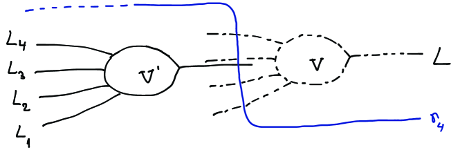
Figure 13. The cobordism $V$, its translation $V^{\prime}$ and the curve $\gamma_{4}$.

In this case, by the same argument showing the point i of Corollary 4.4.3, we deduce $\mathcal{M}_{V^{\prime},\gamma_{m},h_{m}}=\mathcal{Y}(L)$. We put $\phi_{V,\gamma_{m},h_{m}}=e^{\ast}_{\gamma_{m},h_{m}}(\Phi^{V^{\prime}}_{V})$. The invariance part of the statement follows in a way similar to Remark 4.4.4. ∎

Remark 4.5.2.

The map $\phi_{V,\gamma_{m},h_{m}}$ is identified in homology with a map based on counting holomorphic polygons of exactly the same type as the maps $\phi_{V,j}$ from Corollary 4.4.3. This identification is useful in applications. Therefore we will justify this statement in some detail. Consider a curve $\gamma^{\prime}$ as in Figure 14.

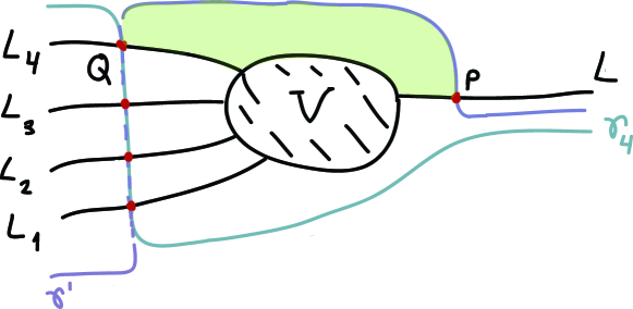
Figure 14. The cobordism $V$, and the curves $\gamma_{4}$ and $\gamma^{\prime}$.

In particular, $\gamma^{\prime}$ coincides with $\gamma_{m}$ as far as the intersections with the negative ends of $V$ are concerned. We will also consider an associated profile function $h^{\prime}$ that is also an extension of $h_{m}$. By the same methods as in the proof of Corollary 4.4.3 we deduce that there is an additional exact triangle:

$$\mathcal{Y}(L)\stackrel{{\scriptstyle\phi_{V,m+1}\ }}{{\longrightarrow}}\mathcal{M}_{V,\gamma_{m},h_{m}}\stackrel{{\scriptstyle i}}{{\longrightarrow}}Z\stackrel{{\scriptstyle p}}{{\longrightarrow}}\mathcal{Y}(L)$$

so that the module $Z=cone(\phi_{V,m+1})$ is acyclic and thus $\phi_{V,m+1}$ is a quasi-isomorphism ($i$ is the inclusion here and $p$ the projection). Geometrically, the module morphism $\phi_{V,m+1}$ counts $J$-polygons with the last entry over $P$ and ending over one of the intersections of $\gamma^{\prime}$ with the negative ends of $V$. It is not hard to see that $\phi_{V,\gamma_{m},h_{m}}$ and $\phi_{V,m+1}$ are homologous. For this we translate again $V$ to $V^{\prime}$ and compare the resulting structures associated to $V,\gamma^{\prime}$ and to $V^{\prime},\gamma^{\prime}$. More precisely, by the same compactness arguments as those used earlier in the paper, we obtain that the following diagram commutes in homology:

(64) $$\begin{aligned} \lx@xy@svg{\hbox{\raise 0.0pt\hbox{\kern 28.41975pt\hbox{\ignorespaces\ignorespaces\ignorespaces\hbox{\vtop{\kern 0.0pt\offinterlineskip\halign{\entry@#!@&&\entry@@#!@\cr&&\\&&\crcr}}}\ignorespaces{\hbox{\kern-16.80031pt\raise 0.0pt\hbox{\hbox{\kern 0.0pt\raise 0.0pt\hbox{\hbox{\kern 3.0pt\raise 0.0pt\hbox{$\textstyle{\mathcal{M}_{V,\gamma_{m},h_{m}}\ignorespaces\ignorespaces\ignorespaces\ignorespaces}$}}}}}}}\ignorespaces\ignorespaces\ignorespaces\ignorespaces{}{\hbox{\lx@xy@droprule}}\ignorespaces\ignorespaces\ignorespaces{\hbox{\kern 29.85132pt\raise 5.30833pt\hbox{{}\hbox{\kern 0.0pt\raise 0.0pt\hbox{\hbox{\kern 3.0pt\hbox{\hbox{\kern 0.0pt\raise-2.30833pt\hbox{$\scriptstyle{i}$}}}\kern 3.0pt}}}}}}\ignorespaces{\hbox{\kern 61.34341pt\raise 0.0pt\hbox{\hbox{\kern 0.0pt\raise 0.0pt\hbox{\lx@xy@tip{1}\lx@xy@tip{-1}}}}}}{\hbox{\lx@xy@droprule}}{\hbox{\lx@xy@droprule}}{\hbox{\kern 61.34341pt\raise 0.0pt\hbox{\hbox{\kern 0.0pt\raise 0.0pt\hbox{\hbox{\kern 3.0pt\raise 0.0pt\hbox{$\textstyle{Z\ignorespaces\ignorespaces\ignorespaces\ignorespaces}$}}}}}}}\ignorespaces\ignorespaces\ignorespaces\ignorespaces{}{\hbox{\lx@xy@droprule}}\ignorespaces\ignorespaces\ignorespaces{\hbox{\kern 97.12437pt\raise 5.1875pt\hbox{{}\hbox{\kern 0.0pt\raise 0.0pt\hbox{\hbox{\kern 3.0pt\hbox{\hbox{\kern 0.0pt\raise-0.8264pt\hbox{$\scriptstyle{p}$}}}\kern 3.0pt}}}}}}\ignorespaces{\hbox{\kern 119.42818pt\raise 0.0pt\hbox{\hbox{\kern 0.0pt\raise 0.0pt\hbox{\lx@xy@tip{1}\lx@xy@tip{-1}}}}}}{\hbox{\lx@xy@droprule}}{\hbox{\lx@xy@droprule}}{\hbox{\kern 119.42818pt\raise 0.0pt\hbox{\hbox{\kern 0.0pt\raise 0.0pt\hbox{\hbox{\kern 3.0pt\raise 0.0pt\hbox{$\textstyle{\mathcal{Y}(L)_{P}}$}}}}}}}{\hbox{\kern-16.69524pt\raise-40.76666pt\hbox{\hbox{\kern 0.0pt\raise 0.0pt\hbox{\hbox{\kern 3.0pt\raise 0.0pt\hbox{$\textstyle{\mathcal{Y}(L)_{Q^{\prime}}\ignorespaces\ignorespaces\ignorespaces\ignorespaces\ignorespaces\ignorespaces\ignorespaces\ignorespaces}$}}}}}}}\ignorespaces\ignorespaces\ignorespaces\ignorespaces{}{\hbox{\lx@xy@droprule}}\ignorespaces\ignorespaces\ignorespaces{\hbox{\kern 29.85132pt\raise-35.45833pt\hbox{{}\hbox{\kern 0.0pt\raise 0.0pt\hbox{\hbox{\kern 3.0pt\hbox{\hbox{\kern 0.0pt\raise-2.30833pt\hbox{$\scriptstyle{i}$}}}\kern 3.0pt}}}}}}\ignorespaces{\hbox{\kern 40.80031pt\raise-40.76666pt\hbox{\hbox{\kern 0.0pt\raise 0.0pt\hbox{\lx@xy@tip{1}\lx@xy@tip{-1}}}}}}{\hbox{\lx@xy@droprule}}{\hbox{\lx@xy@droprule}}\ignorespaces\ignorespaces\ignorespaces\ignorespaces{}{\hbox{\lx@xy@droprule}}\ignorespaces\ignorespaces\ignorespaces{\hbox{\kern-28.41975pt\raise-20.38333pt\hbox{{}\hbox{\kern 0.0pt\raise 0.0pt\hbox{\hbox{\kern 3.0pt\hbox{\hbox{\kern 0.0pt\raise-1.34723pt\hbox{$\scriptstyle{\phi_{V_{m},\gamma_{m},h_{m}}}$}}}\kern 3.0pt}}}}}}\ignorespaces{\hbox{\kern 0.0pt\raise-6.03333pt\hbox{\hbox{\kern 0.0pt\raise 0.0pt\hbox{\lx@xy@tip{1}\lx@xy@tip{-1}}}}}}{\hbox{\lx@xy@droprule}}{\hbox{\lx@xy@droprule}}{\hbox{\kern 40.80031pt\raise-40.76666pt\hbox{\hbox{\kern 0.0pt\raise 0.0pt\hbox{\hbox{\kern 3.0pt\raise 0.0pt\hbox{$\textstyle{cone(id_{\mathcal{Y}(L)})\ignorespaces\ignorespaces\ignorespaces\ignorespaces\ignorespaces\ignorespaces\ignorespaces\ignorespaces}$}}}}}}}\ignorespaces\ignorespaces\ignorespaces\ignorespaces{}{\hbox{\lx@xy@droprule}}\ignorespaces{\hbox{\kern 68.11424pt\raise-3.0pt\hbox{\hbox{\kern 0.0pt\raise 0.0pt\hbox{\lx@xy@tip{1}\lx@xy@tip{-1}}}}}}{\hbox{\lx@xy@droprule}}{\hbox{\lx@xy@droprule}}\ignorespaces\ignorespaces\ignorespaces\ignorespaces{}{\hbox{\lx@xy@droprule}}\ignorespaces\ignorespaces\ignorespaces{\hbox{\kern 97.12437pt\raise-35.57916pt\hbox{{}\hbox{\kern 0.0pt\raise 0.0pt\hbox{\hbox{\kern 3.0pt\hbox{\hbox{\kern 0.0pt\raise-0.8264pt\hbox{$\scriptstyle{p}$}}}\kern 3.0pt}}}}}}\ignorespaces{\hbox{\kern 119.42818pt\raise-40.76666pt\hbox{\hbox{\kern 0.0pt\raise 0.0pt\hbox{\lx@xy@tip{1}\lx@xy@tip{-1}}}}}}{\hbox{\lx@xy@droprule}}{\hbox{\lx@xy@droprule}}{\hbox{\kern 119.42818pt\raise-40.76666pt\hbox{\hbox{\kern 0.0pt\raise 0.0pt\hbox{\hbox{\kern 3.0pt\raise 0.0pt\hbox{$\textstyle{\mathcal{Y}(L)_{P}\ignorespaces\ignorespaces\ignorespaces\ignorespaces}$}}}}}}}\ignorespaces\ignorespaces\ignorespaces\ignorespaces{}{\hbox{\lx@xy@droprule}}\ignorespaces\ignorespaces\ignorespaces{\hbox{\kern 123.60141pt\raise-20.38333pt\hbox{{}\hbox{\kern 0.0pt\raise 0.0pt\hbox{\hbox{\kern 3.0pt\hbox{\hbox{\kern 0.0pt\raise-2.43056pt\hbox{$\scriptstyle{id}$}}}\kern 3.0pt}}}}}}\ignorespaces{\hbox{\kern 135.6564pt\raise-5.5pt\hbox{\hbox{\kern 0.0pt\raise 0.0pt\hbox{\lx@xy@tip{1}\lx@xy@tip{-1}}}}}}{\hbox{\lx@xy@droprule}}{\hbox{\lx@xy@droprule}}\ignorespaces}}}}\ignorespaces\end{aligned} \textstyle{\mathcal{M}_{V,\gamma_{m},h_{m}}\ignorespaces\ignorespaces\ignorespaces\ignorespaces} \scriptstyle{i} \textstyle{Z\ignorespaces\ignorespaces\ignorespaces\ignorespaces} \scriptstyle{p} \textstyle{\mathcal{Y}(L)_{P}} \textstyle{\mathcal{Y}(L)_{Q^{\prime}}\ignorespaces\ignorespaces\ignorespaces\ignorespaces\ignorespaces\ignorespaces\ignorespaces\ignorespaces} \scriptstyle{i} \scriptstyle{\phi_{V_{m},\gamma_{m},h_{m}}} \textstyle{cone(id_{\mathcal{Y}(L)})\ignorespaces\ignorespaces\ignorespaces\ignorespaces\ignorespaces\ignorespaces\ignorespaces\ignorespaces} \scriptstyle{p} \textstyle{\mathcal{Y}(L)_{P}\ignorespaces\ignorespaces\ignorespaces\ignorespaces} \scriptstyle{id} \textstyle{\mathcal{M}_{V,\gamma_{m},h_{m}}\ignorespaces\ignorespaces\ignorespaces\ignorespaces} \scriptstyle{i} \textstyle{Z\ignorespaces\ignorespaces\ignorespaces\ignorespaces} \scriptstyle{p} \textstyle{\mathcal{Y}(L)_{P}} \textstyle{\mathcal{Y}(L)_{Q^{\prime}}\ignorespaces\ignorespaces\ignorespaces\ignorespaces\ignorespaces\ignorespaces\ignorespaces\ignorespaces} \scriptstyle{i} \scriptstyle{\phi_{V_{m},\gamma_{m},h_{m}}} \textstyle{cone(id_{\mathcal{Y}(L)})\ignorespaces\ignorespaces\ignorespaces\ignorespaces\ignorespaces\ignorespaces\ignorespaces\ignorespaces} \scriptstyle{p} \textstyle{\mathcal{Y}(L)_{P}\ignorespaces\ignorespaces\ignorespaces\ignorespaces} \scriptstyle{id}$$

Here the vertical arrows are induced by translating from $V^{\prime}$ to $V$ and $\mathcal{Y}(L)_{P}$ represents the module $\mathcal{Y}(L)$ associated to the point $P\in\gamma^{\prime}$ and $\mathcal{Y}(L)_{Q^{\prime}}$ represents the module $\mathcal{Y}(L)$ associated to the point $Q^{\prime}$ which is the leftmost intersection of $\gamma^{\prime}$ and $V^{\prime}$ - as in Figure 15. This notation is based on the decomposition (as vector spaces) $CF(\gamma^{\prime}\times N,V)=CF(N,L)\oplus\mathcal{M}_{V,\gamma_{m},h_{m}}(N)$ for $N\in\mathcal{L}^{\ast}_{d}(M)$ where the first term corresponds to generators that project to $P$ and so we denote it by $\mathcal{Y}(L)_{P}$. A similar convention is applied to $V^{\prime}$ and $\gamma^{\prime}$ relative to the point $Q^{\prime}$.

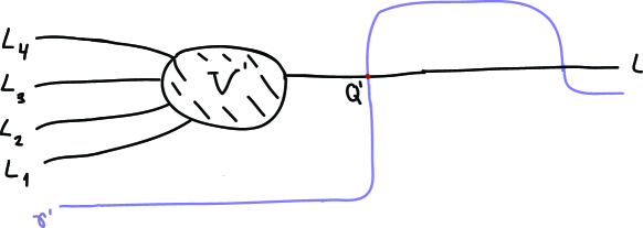
Figure 15. The cobordism $V^{\prime}$, and the curves $\gamma^{\prime}$.

By extending the top and bottom exact sequences one more step to the right we obtain that in homology $[\phi_{V,\gamma_{m},h_{m}}]=[\phi_{V,m+1}]$.

4.6. Definition of $\widetilde{\mathcal{F}}$

The functor

$$\widetilde{\mathcal{F}}:\mathcal{C}ob_{0}^{d}(M)\to T^{s}D\mathcal{F}uk^{d}(M)$$

is defined on objects by $\widetilde{\mathcal{F}}(L_{1},\ldots,L_{m})=(L_{1},\ldots,L_{m})$. To define it on morphisms, recall that the morphisms in $\mathcal{C}ob_{0}^{d}(M)$ are obtained from cobordisms of the type $V:N\leadsto(K_{1},\ldots,K_{r})$, $V\in\mathcal{L}_{d}(\mathbb{C}\times M)$ in the following way. We consider disjoint unions of such $V$’s, say $W=V_{1}\cup V_{2}\ldots\cup V_{r}$ and take the horizontal isotopy class $[W]$ of $W$. An additional equivalence relation is used so as to identify cobordisms in case some of the ends of $W$ are void - as described in §2.3: in short, each morphism of $\mathcal{C}ob_{0}^{d}(M)$ is represented by a unique isotopy class of a cobordism $W$ as above so that all the negative ends and all positive ends of $W$ are non-void and are as in Definition 2.2.1 except if there is a single positive end which is void and/or there is a single negative end which is void (both can occur at the same time, for instance if $W$ is void).

To define $\widetilde{\mathcal{F}}$ on morphisms we will use the definition of the category $T^{s}D\mathcal{F}uk^{d}(M)$ as given in §2.6. However, we emphasize that we work here in an ungraded setting. We will first assume that $W$ has a single connected component $W=V$ and that $V:L\leadsto(L_{1},\ldots,L_{m})$. By the results in §4.4.2 and §4.5, we can associate to this cobordism a triple:

$$(\phi_{V,\gamma_{m},h_{m}},\mathcal{M}_{V,\gamma_{m},h_{m}},\eta_{V,\gamma_{m},h_{m}})$$

where $\phi_{V,\gamma_{m},h_{m}}:\mathcal{Y}(L)\to\mathcal{M}_{V,\gamma_{m},h_{m}}$ is the quasi-isomorphism given by Proposition 4.5.1 and $\eta_{V,\gamma_{m},h_{m}}$ is the cone-decompositions (61). This triple depends on $\gamma_{m}$, $h_{m}$ as well as on all the other auxiliary data required in the construction. However, the invariance properties of these structures (see Remark 4.4.4 and Proposition 4.5.1) imply that if we take the image $([\phi_{V,\gamma_{m},h_{m}}],[\mathcal{M}_{V,\gamma_{m},h_{m}}],[\eta_{V,\gamma_{m},h_{m}}])$ of this triple inside the derived Fukaya category (or $T^{s}D\mathcal{F}uk^{d}(M)$) and compare it with the triple $([\phi_{V^{\prime},\gamma^{\prime}_{m},h^{\prime}_{m}}],[\mathcal{M}_{V,^{\prime}\gamma^{\prime}_{m},h^{\prime}_{m}}],[\eta_{V^{\prime},\gamma^{\prime}_{m},h^{\prime}_{m}}])$ associated to some $V^{\prime}$ horizontally isotopic to $V$ as well as to $\gamma^{\prime}_{m}$, $h^{\prime}_{m}$ etc, then the two triples are related precisely by the equivalence described by (12) in §2.6. Notice also that the linearization of $[\eta_{V,\gamma_{m},h_{m}}]$ is $(L_{1},\ldots,L_{m})$ again by (61) (here $L_{i}$ and $\mathcal{Y}(L_{i})$ are identified, of course).

Therefore, $([\phi_{V,\gamma_{m},h_{m}}],[\mathcal{M}_{V,\gamma_{m},h_{m}}],[\eta_{V,\gamma_{m},h_{m}}])$ determines a morphism

$$\overline{([\phi_{V,\gamma_{m},h_{m}}],[\mathcal{M}_{V,\gamma_{m},h_{m}}],[\eta_{V,\gamma_{m},h_{m}}])}:L\to(L_{1},\ldots,L_{m})$$

in $T^{S}D\mathcal{F}uk^{d}(M)$ that depends only on the horizontal isotopy class of $V$.

We then put:

(65) $$\widetilde{\mathcal{F}}(V)=\overline{([\phi_{V,\gamma_{m},h_{m}}],[\mathcal{M}_{V,\gamma_{m},h_{m}}],[\eta_{V,\gamma_{m},h_{m}}])}~{}.~{}$$

The next step is to pass to the more general case of a disconnected $W$. In this case we notice that both the domain and target categories are strictly monoidal and we extend the definition of $\widetilde{\mathcal{F}}$ monoidally.

Remark 4.6.1.

It is immediate to see that this definition is in fact compatible with the geometry of the cone-decompositions given in Corollary 4.4.3 and of that of the maps $\phi_{{V},\gamma_{m},h_{m}}$ from Proposition 4.5.1. In other words, if we apply the constructions in §4.4.2 and §4.5 to a disconnected cobordism we obtain cone-decompositions and comparison maps between the ends that are the sums of the respective structures for each component at a time. Indeed, this is a direct reflection of the fact that a complex of the form $CF^{cob}(\gamma_{m}\times N,W)$ for $W=V_{1}\cup\cdots\cup V_{r}$ with $V_{i}$ connected splits as

$$CF^{cob}(\gamma_{m}\times N,W)=CF^{cob}(\gamma_{m}\times N,V_{1})\oplus\cdots\oplus CF^{cob}(\gamma_{m}\times N,V_{r}).$$

4.7. Compatibility with composition

It is easy to see that $\widetilde{\mathcal{F}}$ takes a trivial cobordism to the identity (see §2.6). Thus, to show that $\widetilde{\mathcal{F}}$ is a functor, it remains to prove that it is compatible with composition.

Consider two connected cobordisms: $V:L\to(L_{1},\ldots,L_{m})$ and $V^{\prime}:L_{i}\to(L^{\prime}_{1},\ldots,L^{\prime}_{q})$, where $1\leq i\leq m$.

To fix ideas, assume that $V\subset[0,1]\times\mathbb{R}\times M$ and that (after a possible rescaling) $V^{\prime}\subset[0,a]\times[1,q]\times M$ with $a>2$. We also assume that $V^{\prime}$ is cylindrical over $[a-1,a]\times\mathbb{R}$ as well as over $[0,1]\times\mathbb{R}$. We now consider the cobordism: $V^{\prime\prime}:L\to(L_{1},\ldots,L_{i-1},L^{\prime}_{1},\ldots,L^{\prime}_{q},L_{i+1},\ldots,L_{m})$, $V^{\prime\prime}\subset[-a,1]\times\mathbb{R}\times M$ obtained by gluing $V^{\prime}+(-a,i-1)$ (this is just the translation of $V^{\prime}$ by the vector $(-a,i-1)\in\mathbb{R}^{2}$) to $V$ along the $L_{i}$ end and extending the other negative ends of $V$ by trivial cobordisms of the type $\eta_{j}\times L_{j}$ for $j\not=i$ - see Figure 16.

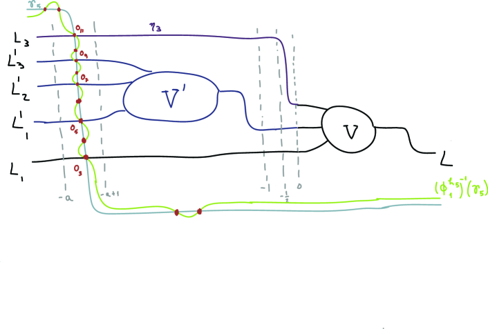
Figure 16. The cobordism $V^{\prime\prime}$ together with the curve $\gamma_{5}$ and the curve $(\phi^{h_{5}}_{1})^{-1}(\gamma_{5})$.

Here the curves $\eta_{j}:[-a,0]\to[-a,0]\times\mathbb{R}$ are so that $\eta_{j}(0)=(0,j)$ for all $j$; for $j\geq i$ we have $\eta_{j}(t)=(t,j+q)$ for all $t\leq-\frac{1}{2}$; $\eta_{j}(t)=(t,j)$, for all $t\leq-\frac{1}{2}$ in case $j<i$. Moreover, we assume that all $\eta_{j}$’s are graphs of functions that have a derivative that is negative or null at all points.

As earlier in the paper, we will actually work in practice with the $\mathbb{R}$-extensions of all the cobordisms involved - see §2.2.

In ${\textnormal{Mor\/}}(\mathcal{C}ob^{d}_{0}(M))$ we have:

(66) $$[V^{\prime\prime}]=(\mathrm{id}_{L_{1}}+\ldots+\mathrm{id}_{L_{i-1}}+[V^{\prime}]+\mathrm{id}_{L_{i+1}}+\ldots+\mathrm{id}_{L_{m}})\circ[V]~{}.~{}$$

Given the definition of the composition in $T^{S}\mathcal{F}uk^{d}(M)$ - see (13) - it follows that it is enough to show that $\widetilde{\mathcal{F}}$ is compatible with compositions of the type in (66). Put $\mathcal{V}^{\prime}=\mathrm{id}_{L_{1}}+\ldots+\mathrm{id}_{L_{i-1}}+[V^{\prime}]+\mathrm{id}_{L_{i+1}}+\ldots+\mathrm{id}_{L_{m}}$. Thus our aim is to show:

Proposition 4.7.1.

With the notation above we have:

$$\widetilde{\mathcal{F}}(V^{\prime\prime})=\widetilde{\mathcal{F}}(\mathcal{V}^{\prime})\circ\widetilde{\mathcal{F}}(V)~{}.~{}$$

Proof.

The first step in the proof is to consider a different cobordism $V^{\prime\prime}_{0}$ that is obtained as follows: first consider the cobordism $V_{0}$ obtained by extending each negative end of $V$ by $[-a,0]\times\{j\}\times L_{j}$ if $j\leq i$ and by $\eta_{j}([-a,0]))\times L_{j}$ if $j>i$. The cobordism $V^{\prime\prime}_{0}$ is obtained by gluing $V^{\prime}$ to $V_{0}$ along the $i$-th end and extending the other ends of $V_{0}$ trivially. In other words:

$$V^{\prime\prime}_{0}=V_{0}\cup\Bigl{(}V^{\prime}+(-2a,i-1)\Bigr{)}\cup\bigcup_{j<i\ \mathrm{or}\ j>i+q}([-2a,-a]\times\{j\}\times L_{j}),$$

see Figure 17.

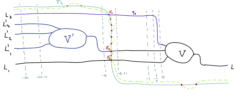
Figure 17. The cobordism $V^{\prime\prime}_{0}$ obtained by translating $V^{\prime}$ to the left by $a$.

Let the $\mathbb{R}$-extensions of $V^{\prime\prime}_{0}$ and $V^{\prime\prime}$ be denoted by $\overline{V}^{\prime\prime}_{0}$ and $\overline{V}^{\prime\prime}$.

It is not difficult to see that there is a horizontal Hamiltonian isotopy $\overline{\psi}_{t}:\mathbb{C}\times M\to\mathbb{C}\times M$, $t\in[0,1]$, of the form $\overline{\psi}_{t}(z,x)=(\psi_{t}(z),x)$ with $\psi_{t}:\mathbb{C}\to\mathbb{C}$ a Hamiltonian isotopy, and with the following properties:

• $\overline{\psi}_{1}(\overline{V}^{\prime\prime})=\overline{V}^{\prime\prime}_{0}$.

• $\psi_{t}$ is the identity on $[-\frac{1}{2},\infty)\times\mathbb{R}$.

• $\psi_{t}$ is a translation in the negative, real direction for all points belonging to $\pi(V^{\prime})\cup[-1,-\frac{1}{2}]\times\{i\}$.

• $\psi_{t}((-\infty,\frac{1}{2}]\times\{j\})=(-\infty,\frac{1}{2}]\times\{j\}$ for all $j>i+q$ as well as all $j<i$. (Recall that $q$ is the number of negative ends of $V^{\prime}$.)

For the next step, put $w=m+q-1$ and we consider a curve $\gamma_{w}$ together with a profile function $h_{w}$ as in §4.4.2 so that the vertical part of $\gamma_{w}$ (i.e. the line that contains the points $o_{j}$ for $3\leq j\leq 2w+1$) is of real coordinate $-a+\frac{1}{2}$ (see Figures 16 and 17). By Remark 4.4.4, this assumption is not restrictive. We also fix all the choices of auxiliary data required to define the category $\mathcal{B}_{\gamma_{w},h_{w}}$ as in §4.2. Recall that we also have the associated category $\mathcal{B}^{\prime}_{w}$ whose objects are the same as those of $\mathcal{B}_{\gamma_{w},h_{w}}$ and whose morphism spaces are quotients of those of $\mathcal{B}_{\gamma_{w},h_{w}}$ as described by (53) in §4.4.2.

By the constructions in §4.4.1, in particular Proposition 4.4.1, we associate to $V^{\prime\prime}$ a sequence of $\mathcal{B}^{\prime}_{w}$-modules, $\mathcal{M}^{*}_{j}$, $j$, $1\leq j\leq w$. With the notation in Proposition 4.4.1, these modules are defined by $\mathcal{M}^{*}_{w}=\mathcal{M}^{\prime}_{w}$ and

$$\mathcal{M}^{*}_{j}=(q_{j+1}\circ\ldots\circ q_{w})^{\ast}(\mathcal{M}^{\prime}_{j})\ \mathrm{for}\ 1\leq j<w~{}.~{}$$

In view of Lemma 4.4.2 these modules admit a direct description: $\mathcal{M}^{\ast}_{w}=\mathcal{M}^{\prime}_{w}$ is the obvious $\mathcal{B}^{\prime}_{w}$-module with $\mathcal{M}^{\ast}_{w}(N)=CF^{cob}(\gamma_{w}\times N,V^{\prime\prime})$ and, for $j<w$, $\mathcal{M}^{\ast}_{j}$ is the sub-module of $\mathcal{M}^{\ast}_{w}$ so that $\mathcal{M}^{\ast}_{j}(N)$ is generated by all the elements in $\mathcal{M}^{\ast}_{w}(N)$ lying over the points $o_{2s+1}$, $s\leq j$. In other words, the generators of $\mathcal{M}^{\ast}_{j}(N)$ correspond to the intersections of $\gamma_{m}$ with the first $j$ ends of $\pi(V^{\prime\prime})$. Thus we obtain inclusions:

(67) $$\mathcal{M}^{\ast}_{1}\to\ldots\to\mathcal{M}^{\ast}_{j-1}\stackrel{{\scriptstyle\kappa_{j}}}{{\longrightarrow}}\mathcal{M}^{\ast}_{j}\stackrel{{\scriptstyle\kappa_{j+1}}}{{\longrightarrow}}\mathcal{M}^{\ast}_{j+1}\to\ldots\to\mathcal{M}^{\ast}_{w}$$

and each $\kappa_{j}$ fits into an exact triangle (that is determined by $\kappa_{j}$ up to isomorphism):

(68) $$Z_{j}\stackrel{{\scriptstyle\phi_{j}}}{{\longrightarrow}}\mathcal{M}^{\ast}_{j-1}\stackrel{{\scriptstyle\kappa_{j}}}{{\longrightarrow}}\mathcal{M}^{\ast}_{j}$$

with:

(69) $$Z_{j}=\begin{cases}(c^{\prime}_{\gamma_{w},h_{w},2j+1})^{\ast}(\mathcal{Y}(L_{j}))&\text{if $j<i$;}\\ (c^{\prime}_{\gamma_{w},h_{w},2j+1})^{\ast}(\mathcal{Y}(L^{\prime}_{j-i+1}))&\text{if $i\leq j\leq i+q-1$;}\\ (c^{\prime}_{\gamma_{w},h_{w},2j+1})^{\ast}(\mathcal{Y}(L_{j-q+1}))&\text{if $i+q\leq j\leq w$.}\end{cases}$$

See §4.2.3 for the definition of the projection $c^{\prime}_{\gamma_{w},h_{w},j}$.

Recall the map $e^{\prime}_{w}:\mathcal{F}uk^{d}(M)\to\mathcal{B}^{\prime}_{w}$ from equation (54). Notice that, in view of Proposition 4.4.1, we have that the sequence of $\mathcal{F}uk^{d}(M)$-modules, $\mathcal{M}_{j}=(e^{\prime}_{w})^{\ast}(\mathcal{M}^{\ast}_{j})$ is identified with the sequence $\mathcal{M}_{V^{\prime\prime},\gamma_{j},h_{j}}$ (where $\gamma_{j},h_{j}$ are constructed, essentially by restricting appropriately $\gamma_{w},h_{w}$). Moreover, the pull-back over $e^{\prime}_{w}$ of the exact triangles (68) are precisely the exact triangles (61). In short, both the module $[\mathcal{M}_{V^{\prime\prime},\gamma_{w},h_{w}}]$ as well as the iterated cone decomposition $[\eta_{V^{\prime\prime},\gamma_{w},h_{w}}]$ are determined by the sequence(67). Next, we define $[\phi_{V^{\prime\prime},\gamma_{w},h_{w}}]$ as follows. Consider the cobordism $V^{\prime\prime}_{1}$ obtained from $V^{\prime\prime}$ by translating it to the left by $2a$. The map $\phi_{V^{\prime\prime},\gamma_{w},h_{w}}$ is then defined to be the pullback over $e^{\prime}_{w}$ of the morphism defined via the “moving boundary” map

$$\Phi^{V^{\prime\prime}_{1}}_{V^{\prime\prime}}:c_{\gamma_{m},h_{m},1}^{\ast}(\mathcal{Y}(L))\to\mathcal{M}^{\ast}_{w}$$

induced by the horizontal isotopy moving $V^{\prime\prime}$ to $V^{\prime\prime}_{1}$.

The sequence of modules (67) has an additional important property. For $1\leq s\leq q$ let $K_{s}$ be the $\mathcal{B}^{\prime}_{w}$ quotient module $K_{s}=\mathcal{M}^{\ast}_{i+s-1}/\mathcal{M}^{\ast}_{i-1}$. They also fit in a sequence of increasing submodules:

(70) $$K_{1}\to\ldots K_{s}\stackrel{{\scriptstyle\l_{s}}}{{\longrightarrow}}K_{s+1}\to\ldots\to K_{q}$$

so that there is a cone decomposition $\eta_{V^{\prime}}$ with exact triangles:

$$Z_{s+i}\to K_{s}\to K_{s+1}~{}.~{}$$

The key property of this cone decomposition is that $\widetilde{\mathcal{F}}(V^{\prime})$ is the equivalence class of the triple $((e^{\prime}_{w})^{\ast}(\phi_{V^{\prime},\gamma_{w},h_{w}}),(e^{\prime}_{w})(K_{q}),(e^{\prime}_{w})(\eta_{V^{\prime}}))$ where $\phi_{V,^{\prime}\gamma_{w},h_{w}}$ is obtained by a moving boundary morphism induced by translating $V^{\prime}$ to the right by $a$ in Figure 17, for instance.

We now intend to show that the cone decomposition $\eta_{V^{\prime\prime},\gamma_{w},h_{w}}$ matches with the cone decomposition associated to $\widetilde{\mathcal{F}}(\mathcal{V}^{\prime})\circ\widetilde{\mathcal{F}}(V)$. To this end, we consider the sequence of $\mathcal{B}^{\prime}_{w}$-modules

(71) $$\mathcal{N}^{\ast}_{1}\to\ldots\mathcal{N}^{\ast}_{j}\stackrel{{\scriptstyle h_{j}}}{{\longrightarrow}}\mathcal{N}^{\ast}_{j+1}\to\ldots\to\mathcal{N}_{w}^{\ast}$$

that are constructed just as the sequence in (68) but by using $V^{\prime\prime}_{0}$ instead of $V^{\prime\prime}$. It is easy to see that all the compactness arguments necessary for the construction of the $\mathcal{M}^{\ast}$’s still apply in this case and that, by an appropriate choice of all the Floer and perturbation data involved we can insure that the modules in (71) satisfy the following properties:

• For $2\leq j\leq w$ there are exact triangles

  $$Z^{\prime}_{j}\stackrel{{\scriptstyle\alpha^{\prime}_{j}}}{{\longrightarrow}}\mathcal{N}^{\ast}_{j-1}\stackrel{{\scriptstyle\tau_{j}}}{{\longrightarrow}}\mathcal{N}^{\ast}_{j}$$

  so that for $2\leq j<i$ or $i+q\leq j\leq w$ we have $Z^{\prime}_{j}=Z_{j}$.

• $Z^{\prime}_{i}=(c^{\prime}_{\gamma_{w},h_{w},2i+1})^{*}(\mathcal{Y}(L_{i}))$ and for $i+1\leq j<i+q$ we have $Z^{\prime}_{j}=0$ and $\tau_{j}=\textnormal{id}$.

• The sequence

  $$\mathcal{N}^{\ast}_{1}\to\ldots\to\mathcal{N}^{\ast}_{i}\to\mathcal{N}^{\ast}_{i+q}\to\ldots\to\mathcal{N}^{\ast}_{w}$$

  pulls back over $e^{\prime}_{w}$ to the respective sequence corresponding to $\widetilde{\mathcal{F}}(V)$.

In view of the composition rule described in §2.2, to show that $\widetilde{\mathcal{F}}(V^{\prime\prime})=\widetilde{\mathcal{F}}(\mathcal{V}^{\prime})\circ\widetilde{\mathcal{F}}(V)$ it is enough to prove that the sequences (67) and (71) are related by morphisms:

$$\xi_{j}:\mathcal{M}^{\ast}_{j}\to\mathcal{N}^{\ast}_{j}$$

so that $\xi_{j}\circ\kappa_{j}=\tau_{j}\circ\xi_{j-1}$ and additionally:

• For $1\leq j<i$, $\xi_{j}=\textnormal{id}$.

• For $j>i+q$, the quotient morphism $\hat{\xi_{j}}:\mathcal{M}^{\ast}_{j}/\mathcal{M}^{\ast}_{j-1}\to\mathcal{N}^{\ast}_{j}/\mathcal{N}^{\ast}_{j-1}$ is the identity.

• For $j=i+q-1$, the quotient morphism

  $$\hat{\xi}_{i+q-1}:K_{q}=\mathcal{M}^{\ast}_{i+q-1}/\mathcal{M}^{\ast}_{i-1}\to\mathcal{N}^{\ast}_{i+q-1}/\mathcal{N}^{\ast}_{i-1}=(c^{\prime}_{\gamma_{w},h_{w},2i+1})^{*}(\mathcal{Y}(L_{i}))$$

  is, in homology, the inverse of the morphism $\phi_{V^{\prime},\gamma_{w},h_{w}}$.

We now want to remark that the module morphisms $\xi_{j}$ with the desired properties are induced by the Hamiltonian isotopy $\overline{\psi}_{t}$. More precisely, consider the morphism:

$$\Psi^{V^{\prime\prime}}_{V^{\prime\prime}_{0}}:\mathcal{M}^{\ast}_{w}\to\mathcal{N}^{\ast}_{w}$$

given by counting $J$-holomorphic polygons with the last edge satisfying a moving boundary condition along the isotopy $\overline{\psi}_{t}$. The principal geometric input at this stage of the proof is that this morphism respects the filtration (67). This follows in view of the properties ii, iii, iv of $\psi_{t}$ combined with arguments similar to those in the proof of Lemma 4.4.2. In essence, we need to show that a curve $u$ belonging to $0$-dimensional moduli space contributing to $\Psi^{V^{\prime\prime}}_{V^{\prime\prime}_{0}}$ that has its last input (the one belonging to $CF^{cob}(\gamma_{m}\times N,V^{\prime\prime})$) of type $o_{k}$ can not have the exit of type $o_{k^{\prime}}$ with $k^{\prime}>k$. Indeed, if such would be the case we see, e.g. by looking at Figures 16, 17, that either $o_{k}$ or $o_{k^{\prime}}$ is left fixed by $\psi_{t}$. Therefore the arguments from the proof of Lemma 4.4.2 apply here and prove analogues of (56) and (57). The properties i’,ii’ follow immediately. Finally, from the definition of $\overline{\psi}_{t}$ it follows that this Hamiltonian isotopy restricted to $V^{\prime}$ is an inverse of the translation inducing $\phi_{V^{\prime},\gamma_{m},h_{m}}$. This implies iii’ and concludes the proof. ∎

4.8. The diagram (1) and the other Corollaries in §1.1

For the convenience of the reader we repeat here Diagram 1 with a slight addition at its bottom that will be explained shortly:

(72) $$\begin{aligned} \lx@xy@svg{\hbox{\raise 0.0pt\hbox{\kern 25.2768pt\hbox{\ignorespaces\ignorespaces\ignorespaces\hbox{\vtop{\kern 0.0pt\offinterlineskip\halign{\entry@#!@&&\entry@@#!@\cr&\\&\\&\crcr}}}\ignorespaces{\hbox{\kern-21.92264pt\raise 0.0pt\hbox{\hbox{\kern 0.0pt\raise 0.0pt\hbox{\hbox{\kern 3.0pt\raise 0.0pt\hbox{$\textstyle{\mathcal{C}ob^{d}_{0}(M)\ignorespaces\ignorespaces\ignorespaces\ignorespaces\ignorespaces\ignorespaces\ignorespaces\ignorespaces}$}}}}}}}\ignorespaces\ignorespaces\ignorespaces\ignorespaces{}{\hbox{\lx@xy@droprule}}\ignorespaces\ignorespaces\ignorespaces{\hbox{\kern 35.06152pt\raise 6.61111pt\hbox{{}\hbox{\kern 0.0pt\raise 0.0pt\hbox{\hbox{\kern 3.0pt\hbox{\hbox{\kern 0.0pt\raise-3.61111pt\hbox{$\scriptstyle{\widetilde{\mathcal{F}}}$}}}\kern 3.0pt}}}}}}\ignorespaces{\hbox{\kern 49.2768pt\raise 0.0pt\hbox{\hbox{\kern 0.0pt\raise 0.0pt\hbox{\lx@xy@tip{1}\lx@xy@tip{-1}}}}}}{\hbox{\lx@xy@droprule}}{\hbox{\lx@xy@droprule}}\ignorespaces\ignorespaces\ignorespaces\ignorespaces{}{\hbox{\lx@xy@droprule}}\ignorespaces\ignorespaces\ignorespaces{\hbox{\kern-10.7639pt\raise-20.69444pt\hbox{{}\hbox{\kern 0.0pt\raise 0.0pt\hbox{\hbox{\kern 3.0pt\hbox{\hbox{\kern 0.0pt\raise-2.39166pt\hbox{$\scriptstyle{\mathcal{P}}$}}}\kern 3.0pt}}}}}}\ignorespaces{\hbox{\kern 0.0pt\raise-29.5pt\hbox{\hbox{\kern 0.0pt\raise 0.0pt\hbox{\lx@xy@tip{1}\lx@xy@tip{-1}}}}}}{\hbox{\lx@xy@droprule}}{\hbox{\lx@xy@droprule}}{\hbox{\kern 49.2768pt\raise 0.0pt\hbox{\hbox{\kern 0.0pt\raise 0.0pt\hbox{\hbox{\kern 3.0pt\raise 0.0pt\hbox{$\textstyle{T^{S}D\mathcal{F}uk^{d}(M)\ignorespaces\ignorespaces\ignorespaces\ignorespaces}$}}}}}}}\ignorespaces\ignorespaces\ignorespaces\ignorespaces{}{\hbox{\lx@xy@droprule}}\ignorespaces\ignorespaces\ignorespaces{\hbox{\kern 81.67862pt\raise-20.69444pt\hbox{{}\hbox{\kern 0.0pt\raise 0.0pt\hbox{\hbox{\kern 3.0pt\hbox{\hbox{\kern 0.0pt\raise-2.39166pt\hbox{$\scriptstyle{\mathcal{P}}$}}}\kern 3.0pt}}}}}}\ignorespaces{\hbox{\kern 81.67862pt\raise-29.5pt\hbox{\hbox{\kern 0.0pt\raise 0.0pt\hbox{\lx@xy@tip{1}\lx@xy@tip{-1}}}}}}{\hbox{\lx@xy@droprule}}{\hbox{\lx@xy@droprule}}{\hbox{\kern-25.2768pt\raise-41.38889pt\hbox{\hbox{\kern 0.0pt\raise 0.0pt\hbox{\hbox{\kern 3.0pt\raise 0.0pt\hbox{$\textstyle{S\mathcal{C}ob^{d}_{0}(M)\ignorespaces\ignorespaces\ignorespaces\ignorespaces\ignorespaces\ignorespaces\ignorespaces\ignorespaces}$}}}}}}}\ignorespaces\ignorespaces\ignorespaces\ignorespaces{}{\hbox{\lx@xy@droprule}}\ignorespaces\ignorespaces\ignorespaces{\hbox{\kern 35.55458pt\raise-35.99722pt\hbox{{}\hbox{\kern 0.0pt\raise 0.0pt\hbox{\hbox{\kern 3.0pt\hbox{\hbox{\kern 0.0pt\raise-2.39166pt\hbox{$\scriptstyle{\mathcal{F}}$}}}\kern 3.0pt}}}}}}\ignorespaces{\hbox{\kern 54.77145pt\raise-41.38889pt\hbox{\hbox{\kern 0.0pt\raise 0.0pt\hbox{\lx@xy@tip{1}\lx@xy@tip{-1}}}}}}{\hbox{\lx@xy@droprule}}{\hbox{\lx@xy@droprule}}\ignorespaces\ignorespaces\ignorespaces\ignorespaces{}{\hbox{\lx@xy@droprule}}\ignorespaces{\hbox{\kern 0.0pt\raise-70.88889pt\hbox{\hbox{\kern 0.0pt\raise 0.0pt\hbox{\lx@xy@tip{1}\lx@xy@tip{-1}}}}}}{\hbox{\lx@xy@droprule}}{\hbox{\lx@xy@droprule}}{\hbox{\kern 54.77145pt\raise-41.38889pt\hbox{\hbox{\kern 0.0pt\raise 0.0pt\hbox{\hbox{\kern 3.0pt\raise 0.0pt\hbox{$\textstyle{D\mathcal{F}uk^{d}(M)\ignorespaces\ignorespaces\ignorespaces\ignorespaces}$}}}}}}}\ignorespaces\ignorespaces\ignorespaces\ignorespaces{}{\hbox{\lx@xy@droprule}}\ignorespaces\ignorespaces\ignorespaces{\hbox{\kern 81.67862pt\raise-62.08333pt\hbox{{}\hbox{\kern 0.0pt\raise 0.0pt\hbox{\hbox{\kern 3.0pt\hbox{\hbox{\kern 0.0pt\raise-1.75pt\hbox{$\scriptstyle{\hom(N,-)}$}}}\kern 3.0pt}}}}}}\ignorespaces{\hbox{\kern 81.67862pt\raise-72.27777pt\hbox{\hbox{\kern 0.0pt\raise 0.0pt\hbox{\lx@xy@tip{1}\lx@xy@tip{-1}}}}}}{\hbox{\lx@xy@droprule}}{\hbox{\lx@xy@droprule}}{\hbox{\kern-23.42957pt\raise-82.77777pt\hbox{\hbox{\kern 0.0pt\raise 0.0pt\hbox{\hbox{\kern 3.0pt\raise 0.0pt\hbox{$\textstyle{M\mathcal{C}ob^{d}_{0}M\ignorespaces\ignorespaces\ignorespaces\ignorespaces}$}}}}}}}\ignorespaces\ignorespaces\ignorespaces\ignorespaces{}{\hbox{\lx@xy@droprule}}\ignorespaces\ignorespaces\ignorespaces{\hbox{\kern 30.65251pt\raise-76.70277pt\hbox{{}\hbox{\kern 0.0pt\raise 0.0pt\hbox{\hbox{\kern 3.0pt\hbox{\hbox{\kern 0.0pt\raise-1.70833pt\hbox{$\scriptstyle{\mathcal{H}F_{N}}$}}}\kern 3.0pt}}}}}}\ignorespaces{\hbox{\kern 65.76192pt\raise-82.77777pt\hbox{\hbox{\kern 0.0pt\raise 0.0pt\hbox{\lx@xy@tip{1}\lx@xy@tip{-1}}}}}}{\hbox{\lx@xy@droprule}}{\hbox{\lx@xy@droprule}}{\hbox{\kern 65.76192pt\raise-82.77777pt\hbox{\hbox{\kern 0.0pt\raise 0.0pt\hbox{\hbox{\kern 3.0pt\raise 0.0pt\hbox{$\textstyle{(\mathcal{V},\times)}$}}}}}}}\ignorespaces}}}}\ignorespaces\end{aligned} \textstyle{\mathcal{C}ob^{d}_{0}(M)\ignorespaces\ignorespaces\ignorespaces\ignorespaces\ignorespaces\ignorespaces\ignorespaces\ignorespaces} \scriptstyle{\widetilde{\mathcal{F}}} \scriptstyle{\mathcal{P}} \textstyle{T^{S}D\mathcal{F}uk^{d}(M)\ignorespaces\ignorespaces\ignorespaces\ignorespaces} \scriptstyle{\mathcal{P}} \textstyle{S\mathcal{C}ob^{d}_{0}(M)\ignorespaces\ignorespaces\ignorespaces\ignorespaces\ignorespaces\ignorespaces\ignorespaces\ignorespaces} \scriptstyle{\mathcal{F}} \textstyle{D\mathcal{F}uk^{d}(M)\ignorespaces\ignorespaces\ignorespaces\ignorespaces} \scriptstyle{\hom(N,-)} \textstyle{M\mathcal{C}ob^{d}_{0}M\ignorespaces\ignorespaces\ignorespaces\ignorespaces} \scriptstyle{\mathcal{H}F_{N}} \textstyle{(\mathcal{V},\times)} \textstyle{\mathcal{C}ob^{d}_{0}(M)\ignorespaces\ignorespaces\ignorespaces\ignorespaces\ignorespaces\ignorespaces\ignorespaces\ignorespaces} \scriptstyle{\widetilde{\mathcal{F}}} \scriptstyle{\mathcal{P}} \textstyle{T^{S}D\mathcal{F}uk^{d}(M)\ignorespaces\ignorespaces\ignorespaces\ignorespaces} \scriptstyle{\mathcal{P}} \textstyle{S\mathcal{C}ob^{d}_{0}(M)\ignorespaces\ignorespaces\ignorespaces\ignorespaces\ignorespaces\ignorespaces\ignorespaces\ignorespaces} \scriptstyle{\mathcal{F}} \textstyle{D\mathcal{F}uk^{d}(M)\ignorespaces\ignorespaces\ignorespaces\ignorespaces} \scriptstyle{\hom(N,-)} \textstyle{M\mathcal{C}ob^{d}_{0}M\ignorespaces\ignorespaces\ignorespaces\ignorespaces} \scriptstyle{\mathcal{H}F_{N}} \textstyle{(\mathcal{V},\times)}$$

The top line is the functor $\widetilde{\mathcal{F}}$ that was constructed in §4.6 and §4.7.

We first provide a detailed description of the categories and functors in diagram (72). We end the section - and the main body of the paper - with the proof of Corollary 1.1.2 which is the only statement from the introduction that does not directly follow from the statement of Theorem B.

4.8.1. The top square in  (72)

The second row in the diagram is obtained from the first one as follows. The category $S\mathcal{C}ob^{d}_{0}(M)$ has as objects Lagrangians $L\in\mathcal{L}^{\ast}_{d}(M)$. The morphisms from $L$ to $L^{\prime}$ are connected cobordisms $V:L\leadsto(L_{1},\ldots,L_{m-1},L^{\prime})$ (with $m\geq 1$ arbitrary) modulo horizontal isotopy. The composition is induced in the obvious way from that in $\mathcal{C}ob^{d}_{0}(M)$. The projection $\mathcal{P}:\mathcal{C}ob^{d}_{0}(M)\to S\mathcal{C}ob^{d}_{0}(M)$ is the projection on the last component, i.e. $\mathcal{P}(K_{1},\ldots,K_{m})=K_{m}$ and similarly for morphisms. (Recall that in $\mathcal{C}ob^{d}_{0}(M)$ some morphisms are represented by disjoint unions of cobordisms.)

On the algebraic side the projection $\mathcal{P}$ is defined in (22). On objects it is again the projection on the last component and, in the language of Corollary 4.4.3, on morphisms it associates to a triple $(\phi_{V,\gamma_{m},h_{m}},\mathcal{M}_{V,\gamma_{m},h_{m}},\eta_{V,\gamma_{m},h_{m}})$ the morphism

$$w_{m}\circ\phi_{V,\gamma_{m},h_{m}}:\mathcal{Y}(L)\longrightarrow\mathcal{Y}(L_{m})$$

where $w_{m}:\mathcal{M}_{V,\gamma_{m},h_{m}}\longrightarrow\mathcal{Y}(L_{m})$ is the morphism fitting in the last exact triangle from  (61):

$$\mathcal{M}_{V,\gamma_{m-1},h_{m-1}}\longrightarrow\mathcal{M}_{V,\gamma_{m},h_{m}}\xrightarrow{w_{m}}\mathcal{Y}(L_{m})~{}.~{}$$

The functor $\mathcal{F}$ is the identity on objects. To define it on morphisms we notice that each morphism $V:L\to L^{\prime}$ in $S\mathcal{C}ob^{d}_{0}(M)$ provides also a morphism $V:L\to(L_{1},\ldots,L_{m-1},L^{\prime})$ in $\mathcal{C}ob^{d}_{0}(M)$ and the functor $\mathcal{F}$ can be defined as $\mathcal{F}([V])=\mathcal{P}\circ\widetilde{\mathcal{F}}([V])$. More explicitly, the morphism $\mathcal{F}([V]):\mathcal{Y}(L)\to\mathcal{Y}(L^{\prime})$ can be also described in one of the following three equivalent ways:

• It is given by the composition

  $$\mathcal{Y}(L)\xrightarrow{\phi_{V,\gamma_{m},h_{m}}}\mathcal{M}_{V,\gamma_{m},h_{m}}\longrightarrow\mathcal{M}_{V,\gamma_{m},h_{m}}/\mathcal{M}_{V,\gamma_{m-1},h_{m-1}}$$

  where the second map is the projection (see Corollary 4.4.3 and Proposition 4.5.1).

• As we are considering here a morphism $\mathcal{Y}(L)\to\mathcal{Y}(L^{\prime})$, it follows from the general properties of the derived Fukaya category that this morphism is determined by a Floer homology class $\alpha_{V}\in HF(L,L^{\prime})$. In view of the moving boundary description of the morphism $\phi_{V,\gamma_{m},h_{m}}$, this class can be defined as the image of the unit in $HF(L,L)$ by the moving boundary morphism

  $$\phi_{V}:CF(L,L)=CF(\gamma_{m}\times L,V^{\prime})\to CF(\gamma_{m}\times L,V)\xrightarrow{\textnormal{proj}}CF(L,L^{\prime})$$

  where the isotopy $V^{\prime}\to V$ is a translation like in Figure 13 ($L^{\prime}=L_{4}$ in that picture) and $proj$ is the projection on the last term in the vector space decomposition

  $$CF(\gamma_{m}\times L,V)=\oplus_{i}CF(L,L_{i})$$

  (by Lemma 4.4.2 $proj$ is a chain map). Thus, $\mathcal{F}(V)=\phi_{V}([L])\in HF(L,L^{\prime})$.

• In view of Remark 4.5.2 and of the point a. the morphism $\phi_{V}$ can also be described in terms of counting the $J$-holomorphic Floer strips with boundary conditions along $\gamma^{\prime}\times L$ and $V$ and having as input an intersection point that projects to the point $P$ in Figure 14 and having as exit a point that projects to $Q$ in the same picture (these strips cover the region filled in color there; the same morphism is discussed in Figure 2).

4.8.2. The bottom square in diagram (72)

The category $M\mathcal{C}ob^{d}_{0}(M)$ is the monoidal completion of $S\mathcal{C}ob^{d}_{0}(M)$, its objects are families $(L_{1},\ldots,L_{k})$ and the morphisms are similar families of morphisms from $S\mathcal{C}ob^{d}_{0}(M)$. We remark that while the objects of $\mathcal{C}ob^{d}_{0}(M)$ and $M\mathcal{C}ob^{d}_{0}(M)$ are the same the morphisms are different.

Given $N\in\mathcal{L}^{\ast}_{d}(M)$, the functor $\mathcal{H}F_{N}$ associates to $(L_{1},\ldots,L_{k})$ the product of Floer homologies $HF(N,L_{1})\times\ldots\times HF(N,L_{k})$. Further, for each cobordism $V:L\to(L_{1},\ldots,L_{i},L^{\prime})$, $\mathcal{H}F_{N}(V)$ is the morphism

$$\mathcal{H}F_{N}(V)=\phi^{N}_{V}:HF(N,L)=HF(\gamma_{m}\times N,V^{\prime})\longrightarrow HF(\gamma_{m}\times N,V)\xrightarrow{\textnormal{proj}}HF(N,L^{\prime})$$

defined by a moving boundary condition as at the point b above. In particular, $\phi_{V}=\mathcal{H}F_{L}(V)$. Alternatively, we can again define this morphism by counting strips as indicated at the point c. above. The commutativity of the bottom square is immediate in this setting.

4.8.3. Proof of Corollary 1.1.2

We will make use of the equivalent descriptions of the functor $\mathcal{F}$ as given at the points a, b, c in §4.8.1. The key point is that for a cobordism $V:L\to(L_{1},\ldots,L^{\prime})$ the morphism $\mathcal{F}(V)\in HF(L,L^{\prime})={\textnormal{Mor\/}}_{D\mathcal{F}uk^{d}(M)}(L,L^{\prime})$ has two equivalent descriptions. One - described at the point a - is a projection composed with the moving boundary comparison morphism associated to a translation of $V$ as in Proposition 4.5.1 and Figure 13. The other - described at the point c - is expressed in terms of counting Floer strips with boundary conditions along $\gamma^{\prime}\times L$ and $V$ where $\gamma^{\prime}$ is a “hat”-like curve as in Figure 14 (see also Remark 4.5.2).

We now specialize to the setting of the Corollary. We use the notation in the statement, in particular, $V,V^{\prime},V^{\prime\prime}$ are as in Figure 3 (for the convenience of the reader, we repeat that Figure below).

We consider the cobordism $V$ and a curve $\gamma_{2}$ as in Figure 18.

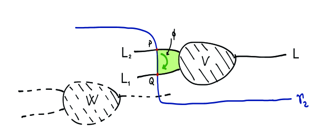
Figure 18. The cobordism $V$, its translated version $W$, the curve $\gamma_{2}$ and the strips giving $\phi$.

As a consequence of Theorem A we deduce the existence of an exact triangle in $D\mathcal{F}uk^{d}(M)$, given as the horizontal line in the next diagram

(73) $$\begin{aligned} \lx@xy@svg{\hbox{\raise 0.0pt\hbox{\kern 7.80278pt\hbox{\ignorespaces\ignorespaces\ignorespaces\hbox{\vtop{\kern 0.0pt\offinterlineskip\halign{\entry@#!@&&\entry@@#!@\cr&&&\\&&&\crcr}}}\ignorespaces{\hbox{\kern-7.80278pt\raise 0.0pt\hbox{\hbox{\kern 0.0pt\raise 0.0pt\hbox{\hbox{\kern 3.0pt\raise 0.0pt\hbox{$\textstyle{L_{2}\ignorespaces\ignorespaces\ignorespaces\ignorespaces}$}}}}}}}\ignorespaces\ignorespaces\ignorespaces\ignorespaces{}{\hbox{\lx@xy@droprule}}\ignorespaces\ignorespaces\ignorespaces{\hbox{\kern 14.71736pt\raise 6.1111pt\hbox{{}\hbox{\kern 0.0pt\raise 0.0pt\hbox{\hbox{\kern 3.0pt\hbox{\hbox{\kern 0.0pt\raise-1.75pt\hbox{$\scriptstyle{\phi}$}}}\kern 3.0pt}}}}}}\ignorespaces{\hbox{\kern 31.80278pt\raise 0.0pt\hbox{\hbox{\kern 0.0pt\raise 0.0pt\hbox{\lx@xy@tip{1}\lx@xy@tip{-1}}}}}}{\hbox{\lx@xy@droprule}}{\hbox{\lx@xy@droprule}}{\hbox{\kern 31.80278pt\raise 0.0pt\hbox{\hbox{\kern 0.0pt\raise 0.0pt\hbox{\hbox{\kern 3.0pt\raise 0.0pt\hbox{$\textstyle{L_{1}\ignorespaces\ignorespaces\ignorespaces\ignorespaces}$}}}}}}}\ignorespaces\ignorespaces\ignorespaces\ignorespaces{}{\hbox{\lx@xy@droprule}}\ignorespaces\ignorespaces\ignorespaces{\hbox{\kern 58.29076pt\raise 5.30833pt\hbox{{}\hbox{\kern 0.0pt\raise 0.0pt\hbox{\hbox{\kern 3.0pt\hbox{\hbox{\kern 0.0pt\raise-2.30833pt\hbox{$\scriptstyle{i\ \ }$}}}\kern 3.0pt}}}}}}\ignorespaces{\hbox{\kern 71.40834pt\raise 0.0pt\hbox{\hbox{\kern 0.0pt\raise 0.0pt\hbox{\lx@xy@tip{1}\lx@xy@tip{-1}}}}}}{\hbox{\lx@xy@droprule}}{\hbox{\lx@xy@droprule}}{\hbox{\kern 71.40834pt\raise 0.0pt\hbox{\hbox{\kern 0.0pt\raise 0.0pt\hbox{\hbox{\kern 3.0pt\raise 0.0pt\hbox{$\textstyle{\mathrm{Cone}(\phi)\ignorespaces\ignorespaces\ignorespaces\ignorespaces}$}}}}}}}\ignorespaces\ignorespaces\ignorespaces\ignorespaces{}{\hbox{\lx@xy@droprule}}\ignorespaces\ignorespaces\ignorespaces{\hbox{\kern 110.5176pt\raise 5.1875pt\hbox{{}\hbox{\kern 0.0pt\raise 0.0pt\hbox{\hbox{\kern 3.0pt\hbox{\hbox{\kern 0.0pt\raise-0.8264pt\hbox{$\scriptstyle{\ \ p}$}}}\kern 3.0pt}}}}}}\ignorespaces{\hbox{\kern 137.36674pt\raise 0.0pt\hbox{\hbox{\kern 0.0pt\raise 0.0pt\hbox{\lx@xy@tip{1}\lx@xy@tip{-1}}}}}}{\hbox{\lx@xy@droprule}}{\hbox{\lx@xy@droprule}}{\hbox{\kern 137.36674pt\raise 0.0pt\hbox{\hbox{\kern 0.0pt\raise 0.0pt\hbox{\hbox{\kern 3.0pt\raise 0.0pt\hbox{$\textstyle{L_{2}}$}}}}}}}{\hbox{\kern-3.0pt\raise-38.41666pt\hbox{\hbox{\kern 0.0pt\raise 0.0pt\hbox{\hbox{\kern 3.0pt\raise 0.0pt\hbox{$\textstyle{}$}}}}}}}{\hbox{\kern 36.60556pt\raise-38.41666pt\hbox{\hbox{\kern 0.0pt\raise 0.0pt\hbox{\hbox{\kern 3.0pt\raise 0.0pt\hbox{$\textstyle{}$}}}}}}}{\hbox{\kern 85.98476pt\raise-38.41666pt\hbox{\hbox{\kern 0.0pt\raise 0.0pt\hbox{\hbox{\kern 3.0pt\raise 0.0pt\hbox{$\textstyle{L\ignorespaces\ignorespaces\ignorespaces\ignorespaces}$}}}}}}}\ignorespaces\ignorespaces\ignorespaces\ignorespaces{}{\hbox{\lx@xy@droprule}}\ignorespaces\ignorespaces\ignorespaces{\hbox{\kern 82.38765pt\raise-19.20833pt\hbox{{}\hbox{\kern 0.0pt\raise 0.0pt\hbox{\hbox{\kern 3.0pt\hbox{\hbox{\kern 0.0pt\raise-1.50694pt\hbox{$\scriptstyle{\sigma}$}}}\kern 3.0pt}}}}}}\ignorespaces{\hbox{\kern 92.38754pt\raise-5.5pt\hbox{\hbox{\kern 0.0pt\raise 0.0pt\hbox{\lx@xy@tip{1}\lx@xy@tip{-1}}}}}}{\hbox{\lx@xy@droprule}}{\hbox{\lx@xy@droprule}}{\hbox{\kern 142.16953pt\raise-38.41666pt\hbox{\hbox{\kern 0.0pt\raise 0.0pt\hbox{\hbox{\kern 3.0pt\raise 0.0pt\hbox{$\textstyle{}$}}}}}}}\ignorespaces}}}}\ignorespaces\end{aligned} \textstyle{L_{2}\ignorespaces\ignorespaces\ignorespaces\ignorespaces} \scriptstyle{\phi} \textstyle{L_{1}\ignorespaces\ignorespaces\ignorespaces\ignorespaces} \scriptstyle{i\ \ } \textstyle{\mathrm{Cone}(\phi)\ignorespaces\ignorespaces\ignorespaces\ignorespaces} \scriptstyle{\ \ p} \textstyle{L_{2}} \textstyle{L\ignorespaces\ignorespaces\ignorespaces\ignorespaces} \scriptstyle{\sigma} \textstyle{L_{2}\ignorespaces\ignorespaces\ignorespaces\ignorespaces} \scriptstyle{\phi} \textstyle{L_{1}\ignorespaces\ignorespaces\ignorespaces\ignorespaces} \scriptstyle{i\ \ } \textstyle{\mathrm{Cone}(\phi)\ignorespaces\ignorespaces\ignorespaces\ignorespaces} \scriptstyle{\ \ p} \textstyle{L_{2}} \textstyle{L\ignorespaces\ignorespaces\ignorespaces\ignorespaces} \scriptstyle{\sigma}$$

together with an isomorphism $\sigma:L\to\mathrm{Cone}(\phi)$ induced by isotoping $V$ to a another cobordism $W$, from one side to the other of the curve $\gamma_{2}$, as in Figure 18 (see also Proposition 4.5.1). Further, the morphism $\phi$ is induced by counting strips with boundary conditions along $\gamma_{2}\times L_{2}$ and $V$, starting at $P$ and ending at $Q$. Moreover, $i$ is the inclusion of $L_{1}$ in $\mathrm{Cone}(\phi)=\mathcal{M}_{V,\gamma_{2}}$ and $p$ is the projection of the cone onto $\mathcal{Y}(L_{2})$ (recall that we neglect grading).

By the description of $\mathcal{F}(-)$ at the point a in §4.8.1, $p\circ\sigma=\mathcal{F}(V)$. To finish the proof of the corollary it suffices to show that in $D\mathcal{F}uk^{d}(M)$ we have $\phi=\mathcal{F}(V^{\prime\prime})$ and $\sigma^{-1}\circ i=\mathcal{F}(V^{\prime})$.

To show the identity $\sigma^{-1}\circ i=\mathcal{F}(V^{\prime})$ we first notice that the composition $\psi=\sigma^{-1}\circ i$ is induced by translating $V$ to $W$ (the inverse of the translation used to define $\sigma$). Further, the same methods as those used in Remark 4.5.2 imply that $\psi$ can also be described by counting strips that start at $R$ and end at $K$ and with boundary conditions along $V$ and $\lambda\times L_{1}$ as in Figure 19.

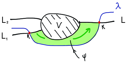
Figure 19. The curve $\lambda$ and the morphism $\psi$.

By the “counting strips” description of $\mathcal{F}(-)$ as at the point c in §4.8.1 it is easy to see, using an appropriate transformation of $\lambda$ as in Figure 20,

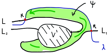
Figure 20. The curve $\lambda$ and the morphism $\psi$ after an appropriate transformation.

that in homology $[\phi_{V^{\prime}}]=[\psi]$.

The identity $\phi=\mathcal{F}(V^{\prime\prime})$ follows by the description of $\mathcal{F}(-)$ in terms of “strip counting”, as at the point c in §4.8.1, and an appropriate transformation of $\gamma_{2}$.

Appendix A Generalities on $A_{\infty}$-categories

We review here basic $A_{\infty}$ notions. All of these are explained in detail in [Sei3]. We recall them for completeness, and also because we use in the paper slightly different conventions (mainly homology rather than cohomology).

In what follows all vector spaces are assumed to be over the field $\mathbb{Z}_{2}$ and are generally ungraded. The algebra below has a graded version (which also works over arbitrary base rings). This requires inserting signs in most of the formulae below (see [Sei3]).

A.1. Extended multilinear maps

Let $I$, $J$ be two sets of indices. Let $\mathbf{C}=\{C_{i,j}\}_{i,j\in I}$, $\mathbf{D}=\{D_{s,r}\}_{s,r\in J}$ be two collections of vector spaces indexed by pairs of indices in $I$ and $J$. An extended multilinear map $F:\mathbf{C}\to\mathbf{D}$ consists of the following. First we have a map $F:I\to J$ which we denote by abuse of notation by $F$. We call it the index map. Next we have a collection of multilinear maps

$$F^{i_{0},\ldots,i_{k}}:C_{i_{0},i_{1}}\otimes\cdots\otimes C_{i_{k-1},i_{k}}\longrightarrow D_{F(i_{0}),F(i_{k})}$$

defined for every $k\geq 1$ and every $i_{0},\ldots,i_{k}\in I$. When it is obvious, we do not specify the index map, e.g. when $I=J$, $\mathbf{C}=\mathbf{D}$ and the index map is the identity (we call this the trivial index map). We often omit the superscripts from $F^{i_{0},\ldots,i_{k}}$ to simplify the notation. We sometimes denote the latter by $F_{k}$ to indicate that it gets $k$ inputs, calling it the degree $k$ part of $F$.

There are two ways to compose extended multilinear maps. Let $F:\mathbf{C}\to\mathbf{D}$ and $G:\mathbf{D}\to\mathbf{E}$ be extended multilinear maps. Define $G\circ F:\mathbf{C}\to\mathbf{E}$ by composing the index maps in an obvious way and

$$(G\circ F)(a_{1},\dots,a_{k})=\sum G(F(a_{1},\ldots,a_{i_{1}-1}),F(a_{i_{1}},\ldots,a_{i_{2}-1}),\ldots,F(a_{i_{l}},\ldots,a_{k}))~{}.~{}$$

The sum is taken over all the possibilities to write terms as on the right-hand side.

For the second type of composition we need to assume that $F:\mathbf{D}\to\mathbf{D}$ (i.e. $\mathbf{C}=\mathbf{D}$) and that the index map of $F$ is the identity. Let $G:\mathbf{D}\to\mathbf{E}$. We define $G\star F:\mathbf{D}\to\mathbf{E}$ by

$$(G\star F)(a_{1},\dots,a_{k})=\sum G(a_{1},\ldots,a_{i-1},F(a_{i},\ldots,a_{l}),a_{l+1},\ldots,a_{k}))~{},~{}$$

where the sum is over all the possibilities to write terms as on the right side above: we apply first $F$ to an ordered subset of the $a_{j}$’s (formed by successive elements) and we use the output of $F$ as one of the inputs for $G$.

We will also need the following generalization. Let $\mathbf{C}=\{C_{i,j}\}_{i,j\in I}$ be a collection of vector spaces as before and $\mathbf{M}=\{M_{i}\}_{i\in I}$, $\mathbf{N}=\{N_{s}\}_{s\in J}$ be two collections of vector spaces indexed by $I$ and $J$. By a mixed extended multilinear map $Q:\mathbf{C}\otimes\mathbf{M}\to\mathbf{N}$ we mean an index map $Q:I\to J$ and a collection of multilinear maps:

$$Q:C_{i_{0},i_{1}}\otimes\cdots\otimes C_{i_{k-2},i_{k-1}}\otimes M_{i_{k-1}}\longrightarrow N_{Q(i_{0})},$$

defined for every $k\geq 1$ and indices $i_{0},\ldots,i_{k-1}\in I$. (Note that for $k=1$ we just have a map $Q:M_{i_{0}}\to M_{i_{0}}$.)

Let $Q:\mathbf{C}\otimes\mathbf{M}\to\mathbf{N}$ be such a map with $\mathbf{N}$ being indexed by the same indices as $\mathbf{M}$ and with identity index map. Let $P:\mathbf{C}\otimes\mathbf{N}\to\mathbf{R}$ be another mixed extended map. We can compose them to get a new mixed extended multilinear map $P\dashv Q:\mathbf{C}\otimes\mathbf{M}\to\mathbf{R}$ as follows:

$$(P\dashv Q)(a_{1},\ldots,a_{k-1},b)=\sum P(a_{1},\ldots,a_{i-1},Q(a_{i},\ldots,a_{k-1},b)).$$

If $F:\mathbf{C}\to\mathbf{C}$ is an extended multilinear map with identity index map and $Q:\mathbf{C}\otimes\mathbf{M}\to\mathbf{N}$ is a mixed extended multilinear map, they can be composed to give a new mixed map $Q\star F:\mathbf{C}\otimes\mathbf{M}\to\mathbf{N}$ as follows:

$$(Q\star F)(a_{1},\dots,a_{k-1},b)=\sum Q(a_{1},\ldots,a_{i-1},F(a_{i},\ldots,a_{l}),a_{l+1},\ldots,a_{k-1},b).$$

A.2. $A_{\infty}$-categories

A.2.1. Definition

An $A_{\infty}$-category $\mathcal{A}$ consists of the following data. A collection of objects $\textnormal{Ob}(\mathcal{A})$, a collection of vector spaces $\mathbf{C}_{\mathcal{A}}=\{C(L^{\prime},L^{\prime\prime})\}_{L^{\prime},L^{\prime\prime}\in\textnormal{Ob}(\mathcal{A})}$ indexed by pairs of objects $L^{\prime},L^{\prime\prime}\in\textnormal{Ob}(\mathcal{A})$, and an extended multilinear map $\mu:\mathbf{C}_{\mathcal{A}}\to\mathbf{C}_{\mathcal{A}}$ (called composition map) with identity index map and which satisfies the identity:

$$\mu\star\mu=0.$$

The space $C(L^{\prime},L^{\prime\prime})$ is called the space of morphisms between $L^{\prime}$ and $L^{\prime\prime}$ and is sometimes denoted by $\hom(L^{\prime},L^{\prime\prime})$. When we want to emphasize the relation to the category $\mathcal{A}$ we write $C_{\mathcal{A}}(L^{\prime},L^{\prime\prime})$ or $\hom_{\mathcal{A}}(L^{\prime},L^{\prime\prime})$.

Note that $\mu_{1}:C(L^{\prime},L^{\prime\prime})\to C(L^{\prime},L^{\prime\prime})$ is a differential, i.e. $\mu_{1}\circ\mu_{1}=0$, hence $C(L^{\prime},L^{\prime\prime})$ becomes a chain complex (ungraded in our case). We denote by $H(L^{\prime},L^{\prime\prime})$ the homology of $(C(L^{\prime},L^{\prime\prime}),\mu_{1})$. The degree $2$ component $\mu_{2}$ of $\mu$ descends to homology and induces an associative product

$$H(L_{0},L_{1})\otimes H(L_{1},L_{2})\longrightarrow H(L_{0},L_{2}),\quad a_{1}\otimes a_{2}\mapsto a_{1}*a_{2}.$$

This means that by passing to homology we obtain a (non-unital) category $H(\mathcal{A})$, called the homology category associated to $\mathcal{A}$. Its objects are $\textnormal{Ob}(\mathcal{A})$, and its morphisms are $\hom_{H(\mathcal{A})}(L,K)=H(L,K)$. The composition of $\alpha\in H(L_{0},L_{1})$, $\beta\in H(L_{1},L_{2})$ is defined to be $\beta\circ\alpha:=\alpha*\beta\in H(L_{0},L_{2})$.

Remark A.2.1.

Notice that our notation is slightly different from that in [Sei3]. The multiplication $\mu_{k}$ in an $A_{\infty}$ algebra is defined for us as

$$\mu_{k}:C(X_{1},X_{2})\otimes C(X_{2},X_{3})\ldots\otimes C(X_{k},X_{k+1})\to C(X_{1},X_{k+1})$$

and in [Sei3] it is defined as a map:

$$C(X_{k},X_{k+1})\otimes C(X_{k-1},X_{k})\ldots\otimes C(X_{1},X_{2})\to C(X_{1},X_{k+1})~{}.~{}$$

As we do not care about signs here the two conventions give the same notion and it is easy to move from one to the other.

A.2.2. Units.

An $A_{\infty}$-category $\mathcal{A}$ is called strictly unital if for every object $L\in\textnormal{Ob}(\mathcal{A})$ there exists a distinguished element $e_{L}\in C(L,L)$ with $\mu_{1}(e_{L})=0$, $\mu_{2}(e_{L},\cdot)=\mu_{2}(\cdot,e_{L})=\textnormal{id}$ and $\mu_{k}(a_{1},\ldots,a_{i-1},e_{L},a_{i+1},\ldots,a_{k})=0$ for every $k\geq 3$ and $1\leq i\leq k$. $\mathcal{A}$ is called homologically unital if for every object $L\in\textnormal{Ob}(\mathcal{A})$ there exists a distinguished element $1_{L}\in H(L,L)$ which behaves like an identity with respect to composition. In most cases considered in the paper the $A_{\infty}$ categories will be homologically unital. Below we will use the following abbreviations: “hu” stands for homologically unital, “su” for strictly unital and “nu” for non-unital (or more precisely, not necessarily unital).

A.2.3. Functors

Let $\mathcal{A}$, $\mathcal{B}$ be two $A_{\infty}$-categories. A nu $A_{\infty}$-functor $\mathcal{F}:\mathcal{A}\to\mathcal{B}$ consists of the following pieces of data. A correspondence which associates for every object $L\in\textnormal{Ob}(\mathcal{A})$ an object $\mathcal{F}(L)\in\textnormal{Ob}(\mathcal{B})$. The second piece is an extended multilinear map $\mathcal{F}:\mathbf{C}_{\mathcal{A}}\to\mathbf{C}_{\mathcal{B}}$ with index map $L\mapsto\mathcal{F}(L)$ and which satisfies the following identity

$$\mathcal{F}\star\mu^{\mathcal{A}}=\mu^{\mathcal{B}}\circ\mathcal{F}.$$

Here $\mu_{\mathcal{A}}$, $\mu_{\mathcal{B}}$ are the composition maps of $\mathcal{A}$, $\mathcal{B}$. Of course, nu $A_{\infty}$-functors $\mathcal{F}$ descend to usual nu functors $H(\mathcal{F}):H(\mathcal{A})\to H(\mathcal{B})$ on the associated homology categories.

Nu $A_{\infty}$-functors $\mathcal{F}:\mathcal{A}\to\mathcal{B}$, $\mathcal{G}:\mathcal{B}\to\mathcal{C}$ can be composed to give a new nu functor $\mathcal{G}\circ\mathcal{F}:\mathcal{A}\to\mathcal{C}$. On the level of objects the composition is obvious and the corresponding extended multilinear maps are composed by using the $\circ$ composition, i.e. $\mathcal{G}\circ\mathcal{F}:\mathbf{C}_{\mathcal{A}}\to\mathbf{C}_{\mathcal{C}}$.

We now describe natural transformations between nu $A_{\infty}$-functors $\mathcal{F},\mathcal{G}:\mathcal{A}\to\mathcal{B}$. First, define a collection of vector spaces $\mathbf{C}_{\mathcal{B}}^{\mathcal{F},\mathcal{G}}=\{C_{\mathcal{A}}(\mathcal{F}(L^{\prime}),\mathcal{G}(L^{\prime\prime}))\}_{L^{\prime},L^{\prime\prime}\in\textnormal{Ob}(\mathcal{A})}$ indexed by pairs of objects of $\mathcal{A}$. A pre-natural transformation $T:\mathcal{F}\to\mathcal{G}$ consists of a pair $T=(T^{0},T^{\prime})$, where $T^{\prime}$ is an extended multilinear map $T^{\prime}:\mathbf{C}_{\mathcal{A}}\to\mathbf{C}_{\mathcal{B}}^{\mathcal{F},\mathcal{G}}$, with identity index map, and $T^{0}$ is a collection of morphisms indexed by $\textnormal{Ob}(\mathcal{A})$, i.e. $T^{0}_{L}\in C_{\mathcal{B}}(\mathcal{F}(L),\mathcal{G}(L)),\,\forall L\in\textnormal{Ob}(\mathcal{A})$.

In order to describe which pre-natural transformations are actually natural we need the following notation. Define $(\mu^{\mathcal{B}}\circ\star\circ(\mathcal{F},T,\mathcal{G})):\mathbf{C}_{\mathcal{A}}\to\mathbf{C}_{\mathcal{B}}^{\mathcal{F},\mathcal{G}}$ to be the following extended multilinear map:

(74) $$(\mu^{\mathcal{B}}\circ\star\circ(\mathcal{F},T,\mathcal{G}))( a_{1},\ldots,a_{k})=$$

$$\sum\mu^{\mathcal{B}}( \mathcal{F}(a_{1},\ldots,a_{q_{1}}),\ldots,\mathcal{F}(a_{q_{j-1}+1}\ldots,a_{q_{j}}),T(a_{q_{j}+1},\ldots,a_{q_{j+1}}),$$

$$\mathcal{G}(a_{q_{j+1}+1},\dots,a_{q_{j+2}}),\ldots,\mathcal{G}(a_{q_{r}+1},\ldots,a_{k})).$$

This sum is taken over all $j$, $r$ and all partitions

$$1\leq q_{1}<\cdots<q_{j}\leq q_{j+1}<\cdots<q_{r}<k.$$

The convention is that if $q_{j}=q_{j+1}$ then the operator $T$ on the right-hand side receives no input so it should be interpreted as $T^{0}_{L_{q_{j}}}\in C(L_{q_{j}},L_{q_{j}})$, while if $q_{j}<q_{j+1}$ the operators $T^{\prime}$ are used.

A pre-natural transformation $T=(T^{0},T^{\prime})$ is called a natural transformation if the following two conditions are satisfied:

(75) $$\mu_{1}^{\mathcal{B}}(T^{0}_{L})=0\quad\forall L\in\textnormal{Ob}(\mathcal{A}),$$

$$(\mu^{\mathcal{B}}\circ\star\circ(\mathcal{F},T,\mathcal{G}))+T^{\prime}\star\mu^{\mathcal{A}}=0.$$

As before, natural transformations between nu $A_{\infty}$-functors induce natural transformations (in the usual sense) between the cohomological functors.

Pre-natural transformations $T=(T^{0},T^{\prime}):\mathcal{F}\to\mathcal{G}$ and $S=(S^{0},S^{\prime}):\mathcal{G}\to\mathcal{H}$ can be composed as follows:

(76) $$(S\circ T)^{0}=\mu_{2}^{\mathcal{B}}(T^{0},S^{0}),$$

$$(S\circ T)^{\prime}=\mu^{\mathcal{B}}\circ\star\circ\star\circ(\mathcal{F},T,\mathcal{G},S,\mathcal{H}),$$

where the operation $\circ\star\circ\star\circ$ should be interpreted in a similar way to (74).

The collection of nu $A_{\infty}$-functors $\mathcal{A}\to\mathcal{B}$ can be given the structure of an $A_{\infty}$-category $\textnormal{\sl nu-fun}(\mathcal{A},\mathcal{B})$. The objects are the nu functors and the morphism spaces $C(\mathcal{F}^{\prime},\mathcal{F}^{\prime\prime})$ are pre-natural transformations between $\mathcal{F}^{\prime}$ and $\mathcal{F}^{\prime\prime}$. The operation $\mu_{1}$ is given by the left-hand side of (75) and $\mu_{2}$ by the right-hand side of (76). The higher $\mu_{k}$’s are given by an obvious generalization of the left-hand side of (75). See [Sei3] for more details. Note that in this language natural transformations are precisely those pre-natural ones $T$ with $\mu_{1}(T)=0$.

Next, we have the notion of a homotopy between two nu $A_{\infty}$-functors. Let $\mathcal{F},\mathcal{G}:\mathcal{A}\to\mathcal{B}$ be two nu $A_{\infty}$-functors with the same action on objects. Consider the pre-natural transformation $D=(0,D^{\prime})$ with $D^{\prime}_{k}=\mathcal{F}_{k}-\mathcal{G}_{k}$ for every $k\geq 1$. A simple calculation shows that $D$ is a natural transformation. We say that $\mathcal{F}$ is homotopic to $\mathcal{G}$ (or that $D$ is homotopic to $0$) if there exists a pre-natural transformation $T=(T^{0},T^{\prime}):\mathcal{F}\to\mathcal{G}$ with $T^{0}=0$ and such that $D=\mu_{1}(T)$. Homotopy is an equivalence relation and is preserved by composition with a given nu functor. Two homotopic nu functors $\mathcal{F}$, $\mathcal{G}$ induce the same functors on the homology categories.

A.2.4. Homologically unital functors

A (nu) $A_{\infty}$-functor $\mathcal{F}:\mathcal{A}\to\mathcal{B}$ between su $A_{\infty}$-categories $\mathcal{A}$, $\mathcal{B}$, is called su if $\mathcal{F}(e_{L})=e_{\mathcal{F}(L)}$ for every $L\in\textnormal{Ob}(\mathcal{A})$ and

$$\mathcal{F}(a_{1},\ldots,a_{i-1},e_{L},a_{i+1},\ldots,a_{k})=0$$

for every $k\geq 2$ and $1\leq i\leq k$.

If $\mathcal{A}$, $\mathcal{B}$ are only hu, a (nu) functor $\mathcal{F}$ is called hu if $H(\mathcal{F}):H(\mathcal{A})\to H(\mathcal{B})$ is a unital functor. We denote by $\textnormal{\sl hu-fun}(\mathcal{A},\mathcal{B})$ the full subcategory of $\textnormal{\sl nu-fun}(\mathcal{A},\mathcal{B})$ consisting of the hu functors. A hu functor $\mathcal{F}$ is called a quasi-equivalence if its homological functor $H(\mathcal{F})$ is an equivalence of categories.

If $\mathcal{A},\mathcal{B}$ are $A_{\infty}$-categories with $\mathcal{B}$ being su then the $A_{\infty}$-categories $\textnormal{\sl hu-fun}(\mathcal{A},\mathcal{B})$ and $\textnormal{\sl nu-fun}(\mathcal{A},\mathcal{B})$ are strictly unital.

A.3. $A_{\infty}$-modules

A.3.1. Basic definition.

Let $Ch$ be the $A_{\infty}$-category of (ungraded) chain complexes of $\mathbb{Z}_{2}$-vector spaces. Objects are chain complexes and morphisms spaces are linear maps between their underlying vector spaces. The operation $\mu_{1}$ is given by the induced differential on maps between two chain complexes, so that $\mu_{1}(f)=0$ iff $f$ is a chain map. The operation $\mu_{2}$ is given by the obvious composition. The higher order composition maps are trivial, i.e. $\mu_{k}=0,\;\forall k\geq 3$, so that $Ch$ is actually a dg-category. We denote by $Ch^{\textnormal{opp}}$ the opposite category. Denoting $C^{\textnormal{opp}}(-,-)$ the morphism spaces for $Ch^{\textnormal{opp}}$ this means that for two chain complexes $C^{\prime}$, $C^{\prime\prime}$ we have $C^{\textnormal{opp}}(C^{\prime},C^{\prime\prime})=\hom(C^{\prime\prime},C^{\prime})$ (the $\hom$ being of vector spaces) endowed with the obvious differential induced from $d_{C^{\prime}}$, $d_{C^{\prime\prime}}$. The operation $\mu_{2}^{\textnormal{opp}}:C(C^{\prime},C^{\prime\prime})\otimes C(C^{\prime\prime},C^{\prime\prime\prime})\to C(C^{\prime},C^{\prime\prime\prime})$ is given by $\mu_{2}^{\textnormal{opp}}(f,g)=g\circ f$. Note that $Ch$ and $Ch^{\textnormal{opp}}$ are strictly unital.

Let $\mathcal{A}$ be an $A_{\infty}$-category. A nu $\mathcal{A}$-module is a nu $A_{\infty}$-functor $\mathcal{M}:\mathcal{A}\to Ch^{\textnormal{opp}}$. The collection of nu $\mathcal{A}$-modules forms a category $\textnormal{\sl nu-mod}_{\mathcal{A}}$ whose objects are nu $\mathcal{A}$-modules, and morphism spaces are pre-natural transformations endowed with the differential $\mu_{1}$ described in the preceding section. The operation $\mu_{2}$ is given by obvious composition and $\mu_{k}=0,\;\forall k\geq 3$.

An alternative more convenient way to describe nu modules is as follows. On the level of objects a nu $\mathcal{A}$-module $\mathcal{M}$ prescribes a collection $\mathbf{M}={\mathcal{M}(L)}_{L\in\textnormal{Ob}(\mathcal{A})}$ of vector spaces indexed by $\textnormal{Ob}(\mathcal{A})$. The second ingredient is a mixed extended multilinear map $\mu_{\mathcal{M}}:\mathbf{C}_{\mathcal{A}}\otimes\mathbf{M}\to\mathbf{M}$ which satisfies the following identity:

(77) $$(\mu^{\mathcal{M}}\dashv\mu^{\mathcal{M}})+(\mu^{\mathcal{M}}\star\mu^{\mathcal{A}})=0.$$

Note that $\mu_{1}^{\mathcal{M}}:\mathcal{M}(L)\to\mathcal{M}(L)$ is a differential, hence $\mathbf{M}$ becomes a collection of chain complexes.

A.3.2. Morphisms.

Pre-module morphisms $\nu:\mathcal{M}^{\prime}\to\mathcal{M}^{\prime\prime}$ between two nu $\mathcal{A}$-modules are given by mixed extended multilinear maps $\nu:\mathbf{C}_{\mathcal{A}}\otimes\mathbf{M}^{\prime}\to\mathbf{M}^{\prime\prime}$. A pre-module morphism $\nu:\mathcal{M}^{\prime}\to\mathcal{M}^{\prime\prime}$ is called a module morphism if

(78) $$(\mu^{\mathcal{M}^{\prime\prime}}\dashv\nu)+(\nu\dashv\mu^{\mathcal{M}^{\prime}})+(\nu\star\mu^{\mathcal{A}})=0.$$

Pre-module morphisms $\nu:\mathcal{M}^{\prime}\to\mathcal{M}^{\prime\prime}$, $\eta:\mathcal{M}^{\prime\prime}\to\mathcal{M}^{\prime\prime\prime}$ can be composed by

(79) $$\eta\dashv\nu:\mathcal{M}^{\prime}\to\mathcal{M}^{\prime\prime\prime}.$$

The collection of nu $\mathcal{A}$-modules $\textnormal{\sl nu-mod}_{\mathcal{A}}$ becomes a dg-category with objects being nu $\mathcal{A}$-modules and morphism spaces $C(\mathcal{M}^{\prime},\mathcal{M}^{\prime\prime})$ being pre-module morphisms $\nu:\mathcal{M}^{\prime}\to\mathcal{M}^{\prime\prime}$. The differential $\mu_{1}$ on $C(\mathcal{M}^{\prime},\mathcal{M}^{\prime\prime})$ is defined by the left-hand side of (78) and the composition $\mu_{2}$ is defined by (79). The higher operations $\mu_{k}$, $k\geq 3$ on $\textnormal{\sl nu-mod}_{\mathcal{A}}$ are defined to be $0$.

There is an identification of $A_{\infty}$-categories $\textnormal{\sl nu-fun}(\mathcal{A},Ch^{\textnormal{opp}})\approx\textnormal{\sl nu-mod}_{\mathcal{A}}$. This goes as follows. If $\mathcal{M}$ is an nu $\mathcal{A}$-module it corresponds to the nu functor $\mathcal{F}:\mathcal{A}\to Ch^{\textnormal{opp}}$ which associates to $L$ the chain complex $(\mathcal{M}(L),\mu_{1}^{\mathcal{M}})$ and with extended multilinear map defined by:

(80) $$\langle\mathcal{F}(a_{1},\ldots,a_{k}),b\rangle=\mu^{\mathcal{M}}(a_{1},\ldots,a_{k},b),$$

$$a_{j}\in C(L_{j-1},L_{j}),\quad b\in C^{\textnormal{opp}}\bigl{(}\mathcal{M}(L_{0}),\mathcal{M}(L_{k})\bigr{)}=\hom(\mathcal{M}(L_{k}),\mathcal{M}(L_{0})).$$

On the level of morphisms the identification is as follows. If $\nu:\mathcal{M}^{\prime}\to\mathcal{M}^{\prime\prime}$ is a pre-module morphism and $\mathcal{F}^{\prime}$, $\mathcal{F}^{\prime\prime}$ are two nu-functors $\mathcal{A}\to Ch^{\textnormal{opp}}$ corresponding to $\mathcal{M}^{\prime}$, $\mathcal{M}^{\prime\prime}$ respectively, then the pre-natural transformation $T=(T^{0},T^{\prime}):\mathcal{F}^{\prime}\to\mathcal{F}^{\prime\prime}$ corresponding to $\nu$ is defined by:

(81) $$T^{0}\in C^{\textnormal{opp}}(\mathcal{M}^{\prime}(L),\mathcal{M}^{\prime\prime}(L))=\hom(\mathcal{M}^{\prime\prime}(L),\mathcal{M}^{\prime}(L)),\quad T^{0}(b)=\nu(b),$$

$$\langle T^{\prime}(a_{1},\ldots,a_{k-1}),b\rangle=\nu(a_{1},\ldots,a_{k-1},b),\quad\forall\,k\geq 2.$$

A.3.3. Pull back of $A_{\infty}$-modules

Let $\phi:\mathcal{A}^{\prime}\to\mathcal{A}$ be a morphism of $A_{\infty}$ categories and let $\mathcal{M}$ be an $A_{\infty}$-module over $\mathcal{A}$. The pull back $\mathcal{M}^{\prime}=\phi^{\ast}\mathcal{M}$ of $\mathcal{M}$ is an $A_{\infty}$ module over $\mathcal{A}^{\prime}$ defined by $\mathcal{M}^{\prime}(X)=\mathcal{M}(\phi(X))$ for each object $X$ of $\mathcal{A}^{\prime}$ and with the higher compositions given by

$$\mu_{\mathcal{M}^{\prime}}(a_{1},\ldots,a_{k},m)=\sum_{i_{1}<i_{2}\ldots}\mu_{\mathcal{M}}(\phi^{i_{1}}(a_{1},\ldots,a_{i_{1}}),\phi^{i_{2}-i_{1}}(a_{i_{1}+1},\ldots,a_{i_{2}}),\ldots,m)~{}.~{}$$

It is easy to check that this is indeed an $A_{\infty}$-module.

A.3.4. Homologically unital modules

Let $\mathcal{A}$ be a hu $A_{\infty}$-category. A hu $\mathcal{A}$-module is a hu $A_{\infty}$-functor $\mathcal{M}:\mathcal{A}\to Ch^{\textnormal{opp}}$. Alternatively, a nu $\mathcal{A}$-module $\mathcal{M}$ is called hu if for every $L\in\textnormal{Ob}(\mathcal{A})$ the homology $H(\mathcal{M}(L),\mu_{1}^{\mathcal{M}})$ is a unital module over the (unital) ring $H(L,L)$. The full subcategory of $\textnormal{\sl nu-mod}_{\mathcal{A}}$ consisting of hu $\mathcal{A}$-modules will be denoted by $\textnormal{hu-mod}_{\mathcal{A}}$. A pull back of a hu module over a morphism of hu $A_{\infty}$ categories is also homologically unital.

Note that since $Ch^{\textnormal{opp}}$ is strictly unital, both $A_{\infty}$-categories $\textnormal{\sl hu-mod}_{\mathcal{A}}$ and $\textnormal{\sl nu-mod}_{\mathcal{A}}$ are strictly unital. The identity module morphism $\nu:\mathcal{M}\to\mathcal{M}$ being the one with $\nu(b)=b$ and $\nu(a_{1},\ldots,a_{k-1},b)=0$ for every $k\geq 1$.

A.4. The Yoneda embedding

Let $\mathcal{A}$ be an $A_{\infty}$-category. The Yoneda functor is the nu $A_{\infty}$-functor $\mathcal{Y}:\mathcal{A}\to\textnormal{\sl nu-mod}_{\mathcal{A}}$, defined as follows. On the level of objects, define $\mathcal{Y}(L):=\mathcal{M}_{L}$, where $\mathcal{M}_{L}$ is the nu module that associates to the object $K\in\textnormal{Ob}(\mathcal{A})$ the vector space $\mathcal{M}_{L}(K)=C_{\mathcal{A}}(K,L)$. The mixed extended multilinear map of $\mathcal{M}_{L}$ is defined as

$$\mu^{\mathcal{M}_{L}}(a_{1},\ldots,a_{k-1},b)=\mu^{\mathcal{A}}(a_{1},\ldots,a_{k-1},b),\quad\forall k\geq 1.$$

The extended multilinear map of the nu functor $\mathcal{Y}$ is described as follows. Let $k\geq 2$ and $L_{0},L_{1},\ldots,L_{k}\in\textnormal{Ob}(\mathcal{A})$. Let $a_{j}\in C_{\mathcal{A}}(L_{j-1},L_{j})$, $j=1,\ldots,k$. We need to specify a pre-module morphism $\mathcal{Y}(a_{1},\ldots,a_{k}):\mathcal{M}_{L_{0}}\to\mathcal{M}_{L_{k}}$. For simplicity of notation we write $\nu=\mathcal{Y}(a_{1},\ldots,a_{k})$. To define $\nu$, let $d\geq 1$ and $K_{0},\ldots,K_{d-1}\in\textnormal{Ob}(\mathcal{A})$. We put

(82) $$\nu:C_{\mathcal{A}}(K_{0},K_{1})\otimes\cdots\otimes C_{\mathcal{A}}(K_{d-2},K_{d-1})\otimes C(K_{d-1},L_{0})\longrightarrow C(K_{0},L_{k}),$$

$$\nu(c_{1},\ldots,c_{d-1},b):=\mu^{\mathcal{A}}(c_{1},\ldots,c_{d-1},b,a_{1},\ldots,a_{k}).$$

The Yoneda functor has better properties for homologically unital categories. Assume that $\mathcal{A}$ is hu. Then the Yoneda functor takes values inside the subcategory of hu modules, $\mathcal{Y}:\mathcal{A}\to\textnormal{\sl hu-mod}_{\mathcal{A}}$. Moreover, the homological functor $H(\mathcal{Y}):H(\mathcal{A})\to H(\textnormal{\sl hu-mod}_{\mathcal{A}})$ is unital and moreover full and faithful. This does not follow immediately from the definitions, and we refer the reader to [Sei3], Section 2g, for the proofs.

Due to its properties in the hu case, we call $\mathcal{Y}$ the Yoneda embedding. Note also that for the $A_{\infty}$-categories that will occur in our applications (Fukaya categories) the Yoneda embedding will generally be injective on objects.

From now on, we will implicitly assume our $A_{\infty}$-categories to be homologically unital unless otherwise stated. For hu functors and modules, we will drop from now on the wording “hu”, calling then simply functors and modules and denoting their respective categories by $\textnormal{\sl fun}(\mathcal{A},\mathcal{B})$ and $\textnormal{\sl mod}_{\mathcal{A}}$.

A.5. Exact triangles and derived categories

Let $\mathcal{A}$ be an $A_{\infty}$-category. Let $\mathcal{M}^{\prime},\mathcal{M}^{\prime\prime}$ be $\mathcal{A}$-modules and $\nu:\mathcal{M}^{\prime}\to\mathcal{M}^{\prime\prime}$ a module morphism. We define a new $\mathcal{A}$-module, $\mathrm{Cone}(\nu)$, called the mapping cone of $\nu$ as follows. On the level of objects $\mathrm{Cone}(\nu)(L)=\mathcal{M}^{\prime}(L)\oplus\mathcal{M}^{\prime\prime}(L)$. The mixed extended multilinear map $\mu^{\mathrm{Cone}(\nu)}$ is defined as

(83) $$\mu^{\mathrm{Cone}(\nu)} (a_{1},\ldots,a_{k-1},(b^{\prime},b^{\prime\prime}))=$$

$$\Bigl{(}\mu^{\mathcal{M}^{\prime}}(a_{1},\ldots,a_{k-1},b^{\prime}),\mu^{\mathcal{M}^{\prime\prime}}(a_{1},\ldots,a_{k-1},b^{\prime\prime})+\nu(a_{1},\ldots,a_{k-1},b^{\prime})\Bigr{)}.$$

The mapping cone comes with two module morphisms: $i:\mathcal{M}^{\prime\prime}\to\mathrm{Cone}(\nu)$ and $\pi:\mathrm{Cone}(\nu)\to\mathcal{M}^{\prime}$ defined by :

(84) $$i_{1}(b^{\prime\prime})=(0,b^{\prime\prime}),\quad i_{k}=0\;\forall\,k\geq 2,$$

$$\pi_{1}(b^{\prime},b^{\prime\prime})=b^{\prime},\quad\pi_{k}=0\;\forall\,k\geq 2.$$

We call the diagram

an exact triangle. We extend the notion of exact triangles to other diagrams as follows. A diagram of $\mathcal{A}$-modules

(85)

(where $\nu$, $j$, $p$ are module morphisms) is called exact if there exists a module morphism $t:\mathcal{C}\to\mathrm{Cone}(\nu)$ such that $[t]:\mathcal{C}\to\mathrm{Cone}(\nu)$ is an isomorphism in the homological category $H(\textnormal{\sl mod}_{\mathcal{A}})$ and such that the following diagram commutes in $H(\textnormal{\sl mod}_{\mathcal{A}})$:

(86)

Note that the $A_{\infty}$-category $\textnormal{\sl mod}_{\mathcal{A}}$ is triangulated in the sense that every module morphism $\nu:\mathcal{M}^{\prime}\to\mathcal{M}^{\prime\prime}$ can be completed to an exact triangle (85).

Remark A.5.1.

As explained in [Sei3] one can generalize the notion of exact triangles in any $A_{\infty}$-category $\mathcal{B}$ (not just for modules). Let $L^{\prime},L^{\prime\prime},L^{\prime\prime\prime}\in\textnormal{Ob}(\mathcal{B})$ and $\nu\in C_{\mathcal{B}}(L^{\prime},L^{\prime\prime})$, $j\in C_{\mathcal{B}}(L^{\prime\prime},L^{\prime\prime\prime})$, $p\in C_{\mathcal{B}}(L^{\prime\prime\prime},L^{\prime})$ be cycles (i.e. $\mu_{1}^{\mathcal{B}}$ vanishes on them). The diagram

is called an exact triangle if its image under the Yoneda embedding is an exact triangle in the sense defined above. In fact, being an exact triangle depends only on the homology classes of $\nu$, $j$, $p$ hence it is a property of diagrams in the homological category $H(\mathcal{B})$. See [Sei3] for more details on that.

Apriori this definition of exact triangles might contradict with the previous one, e.g. if we take $\mathcal{B}=\textnormal{\sl mod}_{\mathcal{A}}$ to start with, then we have two apriori different definitions of exact triangles in $\mathcal{B}$. However, this is not the case (see Corollaries 3.9 and 3.10 in [Sei3]) and the two definitions are actually compatible.

An $A_{\infty}$-category $\mathcal{B}$ is called triangulated if every cycle $\nu\in C_{\mathcal{B}}(L^{\prime},L^{\prime\prime})$ can be completed to an exact triangle. Usually one adds to this an axiom regarding a shift functor. As we are working in the paper in an ungraded framework we can ignore this axiom.

We now briefly recall how to derive an $A_{\infty}$-category. Let $\mathcal{A}$ be an $A_{\infty}$-category (recall that we implicitly assume $\mathcal{A}$ to be homologically unital). Let $\mathcal{Y}:\mathcal{A}\to\textnormal{\sl mod}_{\mathcal{A}}$ be the Yoneda embedding and denote by $\mathcal{Y}(\mathcal{A})$ the image of $\mathcal{A}$.

We now take the triangulated closure of $\mathcal{Y}(\mathcal{A})$ in $\textnormal{\sl mod}_{\mathcal{A}}$, namely a minimal full subcategory $\mathcal{Y}(\mathcal{A})^{\wedge}\subset\textnormal{\sl mod}_{\mathcal{A}}$ with the following properties:

1. $\textnormal{Ob}(\mathcal{Y}(\mathcal{A})^{\wedge})$ is closed under quasi-isomorphisms.

2. $\mathcal{Y}(\mathcal{A})^{\wedge}$ is triangulated.

A constructive realization of $\mathcal{Y}(\mathcal{A})^{\wedge}$ is to first to take the full subcategory (not just homologically) of $\textnormal{\sl mod}_{\mathcal{A}}$ containing the objects of $\mathcal{Y}(\mathcal{A})$ and add all quasi-isomorphic objects to it (plus all morphisms between these new objects and the old ones). Next, form all possible mapping cones between objects of the previous category and then iterate this procedures inductively arbitrary number of times. Finally, one defines the derived category $D(\mathcal{A})$ of $\mathcal{A}$ as the homological category $H\bigl{(}\mathcal{Y}(\mathcal{A})^{\wedge}\bigr{)}$. Note that $D(\mathcal{A})$ is a triangulated category (in the usual sense).

As explained in [Sei3] there are many other realizations of $D(\mathcal{A})$, but they all lead to equivalent categories.

A.6. Families of $A_{\infty}$-categories and equivalences

The discussion here follows Chapter 10 of [Sei3] where one can find more details and proofs.

Let $\mathcal{A}^{i}$, $i\in\mathcal{I}$, be a family of $A_{\infty}$-categories indexed by a set $\mathcal{I}$. Suppose we also have one $A_{\infty}$-category $\mathcal{A}^{\textnormal{tot}}$ such that for every $i\in\mathcal{I}$, $\mathcal{A}^{i}$ is a full $A_{\infty}$-subcategory of $\mathcal{A}^{\textnormal{tot}}$. Denote the embedding functor by $\mathcal{H}^{i}:\mathcal{A}^{i}\to\mathcal{A}^{\textnormal{tot}}$. We assume further that each $\mathcal{H}^{i}$ is a quasi-equivalence. Under these assumption there exists a family of quasi equivalences $\mathcal{K}^{i}:\mathcal{A}^{\textnormal{tot}}\to\mathcal{A}^{i}$, with $\mathcal{K}^{i}\circ\mathcal{H}^{i}=\textnormal{Id}_{\mathcal{A}^{i}}$ for every $i\in\mathcal{I}$. Moreover, the family $\mathcal{A}^{i}$, $i\in\mathcal{I}$, admits a structure of a so called coherent system of $A_{\infty}$-categories (see [Sei3] for the precise definition). In particular we obtain a family of quasi-equivalences $\mathcal{F}^{i_{1},i_{0}}:\mathcal{A}^{i_{0}}\to\mathcal{A}^{i_{1}}$ for every $i_{0},i_{1}\in\mathcal{I}$ with $\mathcal{F}^{i,i}=\textnormal{Id}_{\mathcal{A}^{i}}$ and such that $\mathcal{F}^{i_{2},i_{1}}\circ\mathcal{F}^{i_{1},i_{0}}\cong\mathcal{F}^{i_{2},i_{0}}$, where $\cong$ means that the two functors are isomorphic via a natural transformation. We call the $A_{\infty}$-functors $\mathcal{F}^{i_{1},i_{0}}$ comparison functors.

Passing to the derived categories $D(\mathcal{A}^{i})$, $i\in\mathcal{I}$, we obtain a coherent system of (ordinary) categories with equivalences $F^{i_{1},i_{0}}:D(\mathcal{A}^{i_{0}})\to D(\mathcal{A}^{i_{1}})$ induced from the $\mathcal{F}^{i_{1},i_{0}}$’s. Moreover, the homology level functors $H(\mathcal{K}^{i}):H(\mathcal{A}^{\textnormal{tot}})\to H(\mathcal{A}^{i})$ induced by the $\mathcal{K}^{i}$’s uniquely determine the equivalences $F^{i_{1},i_{0}}$.

Of course, the same applies not only to the derived categories $D(\mathcal{A}^{i})$, $i\in\mathcal{I}$, but also to the homological categories $H(\mathcal{A}^{i})$ (which can be viewed as full subcategories of $D(\mathcal{A}^{i})$). Namely, $H(\mathcal{A}^{i})$, $i\in\mathcal{I}$, becomes a coherent system of categories via the same comparison functors $F^{i_{1},i_{0}}$.

References

- [Abo] M. Abouzaid. Homogeneous coordinate rings and mirror symmetry for toric varieties. Geom. Topol., 10:1097–1157 (electronic), 2006.
- [Arn1] V. Arnol′d. Lagrange and Legendre cobordisms. I. Funktsional. Anal. i Prilozhen., 14(3):1–13, 96, 1980.
- [Arn2] V. Arnol′d. Lagrange and Legendre cobordisms. II. Funktsional. Anal. i Prilozhen., 14(4):8–17, 95, 1980.
- [AS] M. Abouzaid and P. Seidel. An open String Analogue of Viterbo Functoriality. Geom. Topol., 14, 2010.
- [Aur] D. Auroux. Fukaya categories of symmetric products and bordered Heegaard-Floer homology. J. Gökova Geom. Topol. GGT, 4:1–54, 2010.
- [BC1] P. Biran and O. Cornea. Rigidity and uniruling for Lagrangian submanifolds. Geom. Topol., 13(5):2881–2989, 2009.
- [BC2] P. Biran and O. Cornea. Lagrangian cobordism. I. J. Amer. Math. Soc., 26(2):295–340, 2013.
- [CC] F. Charette and O. Cornea. Categorification of Seidel’s representation. Preprint (2013). To appear in Israel Journal of Math. Can be found at http://arxiv.org/pdf/1307.7235v2.
- [Cha] F. Charette. Quelques propriétés des sous-variétés lagrangiennes monotones : Rayon de Gromov et morphisme de Seidel. PhD thesis. PhD, University of Montreal, may 2012.
- [dSRS] V. de Silva, J. Robbin, and D. Salamon. Combinatorial Floer homology, volume 230 of Memoirs of the American Mathematical Society. Amer. Math. Soc., Providence, RI.
- [Flo] A. Floer. Morse theory for Lagrangian intersections. J. Differential Geom., 28(3):513–547, 1988.
- [FOOO1] K. Fukaya, Y.-G. Oh, H. Ohta, and K. Ono. Lagrangian intersection Floer theory: anomaly and obstruction. Part I, volume 46 of AMS/IP Studies in Advanced Mathematics. American Mathematical Society, Providence, RI, 2009.
- [FOOO2] K. Fukaya, Y.-G. Oh, H. Ohta, and K. Ono. Lagrangian intersection Floer theory: anomaly and obstruction. Part II, volume 46 of AMS/IP Studies in Advanced Mathematics. American Mathematical Society, Providence, RI, 2009.
- [Fuk1] K. Fukaya. Morse homotopy, -category, and Floer homologies. In Proceedings of GARC Workshop on Geometry and Topology ’93 (Seoul, 1993), volume 18 of Lecture Notes Ser., pages 1–102, Seoul, 1993. Seoul Nat. Univ.
- [Fuk2] K. Fukaya. Morse homotopy and its quantization. In Geometric topology (Athens, GA, 1993), volume 2.1 of AMS/IP Stud. Adv. Math., pages 409–440, Providence, RI, 1997. Amer. Math. Soc., Amer. Math. Soc.
- [GM] S. Gelfand and Y.I. Manin. Methods of homological algebra. Springer Monographs in Mathematics. Springer-Verlag, Berlin, second edition, 2003.
- [Gro] M. Gromov. Pseudoholomorphic curves in symplectic manifolds. Invent. Math., 82(2):307–347, 1985.
- [Hau1] L. Haug. The lagrangian cobordism group of . Preprint (2013). Can be found at http://arxiv.org/pdf/1310.8056v2.
- [Hau2] L. Haug. On Lagrangian quantum homology and Lagrangian cobordisms. PhD thesis, ETH - Zürich, 2014.
- [HL] S. Hu and F. Lalonde. A relative seidel morphism and the albers map. Trans. Amer. Math. Soc., 362:1135–1168, 2010.
- [HLL] S. Hu, F. Lalonde, and R. Leclercq. Homological lagrangian monodromy. Geom. Topol., 15:1617–1650, 2011.
- [Kon] M. Kontsevich. Homological algebra of mirror symmetry. In Proceedings of the International Congress of Mathematicians, Vol. 1, 2 (Zürich, 1994), pages 120–139, Basel, 1995. Birkhäuser.
- [Lec] R. Leclercq. Spectral invariants in lagrangian floer theory. J. Mod. Dyn., 2:249–286, 2008.
- [MS1] D. McDuff and D. Salamon. -holomorphic curves and symplectic topology, volume 52 of American Mathematical Society Colloquium Publications. American Mathematical Society, Providence, RI, 2004.
- [MS2] D. McDuff and D. Salamon. -holomorphic curves and symplectic topology, volume 52 of American Mathematical Society Colloquium Publications. American Mathematical Society, Providence, RI, second edition, 2012.
- [NT] D. Nadler and H.L. Tanaka. A stable infinity-category of lagrangian cobordisms. Preprint (2011). Can be found at http://arxiv.org/pdf/1109.4835v1.
- [Oh1] Y.-G. Oh. Floer cohomology of Lagrangian intersections and pseudo-holomorphic disks. I. Comm. Pure Appl. Math., 46(7):949–993, 1993.
- [Oh2] Y.-G. Oh. Addendum to: ”Floer cohomology of Lagrangian intersections and pseudo-holomorphic disks. I.” [Comm. Pure Appl. Math. 46 (1993), no. 7, 949–993]. Comm. Pure Appl. Math., 48(11):1299–1302, 1995.
- [Oh3] Y.-G. Oh. Floer cohomology, spectral sequences, and the Maslov class of Lagrangian embeddings. Internat. Math. Res. Notices, 1996(7):305–346, 1996.
- [Oh4] Y.-G. Oh. Floer homology and its continuity for non-compact Lagrangian submanifolds. Turkish J. Math., 25(1):103–124, 2001.
- [Sei1] P. Seidel. of symplectic automorphism groups and invertibles in quantum homology rings. Geom. Funct. Anal., 7(6):1046–1095, 1997.
- [Sei2] P. Seidel. Graded Lagrangian submanifolds. Bull. Soc. Math. France, 128(1):103–149, 2000.
- [Sei3] P. Seidel. Fukaya categories and Picard-Lefschetz theory. Zurich Lectures in Advanced Mathematics. European Mathematical Society (EMS), Zürich, 2008.
- [Sei4] P. Seidel. Fukaya -structures associated to Lefschetz fibrations. I. J. Symplectic Geom., 10(3):325–388, 2012.
- [Wei] A. Weibel. An introduction to homological algebra, volume 38 of Cambridge Studies in Advanced Mathematics. Cambridge University Press, Cambridge, 1994.