Minimal Model for an Unbalanced Holographic Superconductor

Abstract:

We describe the simplest holographic model for an s-wave unbalanced superconductor in $2+1$ dimensions. We study its phase diagram and linear response features with particular attention to the possibility of spatially modulated phases (LOFF) and mixed spin-electric properties. The normal phase of the model at hand allows us to analyze a strong-coupling generalization of Mott two-current model for spintronic systems; the superconducting phase features an interesting DC spin-superconductivity without spin-symmetry breaking .

1 Introduction

1.1 Theoretical framework

The dynamics of quantum field theory at strong coupling has always represented a tough subject to be studied. Especially because it is troublesome to access the strongly coupled regime of QFT by means of standard methods, generally based on perturbation theory. Even adopting numerical lattice methods, the analysis of finite density systems and transport properties is in general particularly delicate and difficult. However, in the last fifteen years, new theoretical insight inspired by string theory and brane dynamics has opened a new theoretical path to the quantitative study of QFT at strong coupling. Such an alternative approach is referred to with the term holography as it is based on a conjectured duality between specific examples of QFT and suitable gravitational models living in a spacetime with higher dimensionality. The paradigmatic example of holographic correspondence is the $AdS$/CFT [2, 3].

Holographic dualities conjecture a correspondence between a QFT (without gravity) and a gravitational model; the former is generally thought of as living on the “boundary” of a bulk manifold where instead the dual gravitational model is defined. The practical power of holography descends from the fact that the strongly coupled regime of the QFT is mapped to the semiclassical regime of the dual gravity model. In other terms, a semiclassical approach based on the direct solution of the equations of motion on the gravity side allows one to obtain quantitative information about the correlation functions of the boundary field theory.

The holographic framework, or gauge/gravity correspondence, has been widely and deeply considered for a plethora of applications like the physics of strongly coupled plasmas and the quantum phase transitions. A more specific but nevertheless very important field of application is the one concerning holographic superconductors [4, 5, 6]. The holographic superconductors are strongly coupled systems manifesting symmetry breaking phenomena which lead to superconductivity; they are useful toy models to study unconventional (non-BCS) superconductivity and possibly shed light on some features of the high-$T_{c}$ superconductivity mechanisms. They implement in a holographic context the essential ingredients to describe the breaking of an Abelian symmetry and the consequent superconducting phenomenon; the minimal model contains a bulk vector gauge field and a charged scalar living in a black hole (i.e. finite temperature) background. The condensation of the charged scalar, namely the black hole hair formation, gives rise to a bulk Higgs mechanism. From the dual standpoint, this condensation is interpreted as the phase transition leading to a strongly coupled superfluid whose one and two-point correlation functions coincide with those of a strongly coupled superconductor.

1.2 Motivations

In [1] we extended the minimal model for a holographic superconductor [6] by introducing a second $U(1)$ gauge field in the bulk theory. This generalization aims at describing a boundary system with two chemical species associated with two chemical potentials. Indeed, following the so-called holographic dictionary, a gauge symmetry in the bulk is related to a conserved current in the boundary and, more specifically, the boundary condition for the time component of the bulk gauge field is interpreted as a chemical potential in the boundary theory.

Having a system with two chemical potentials allows us to study the so-called unbalanced systems characterized by the presence of a chemical imbalance between different chemical species. This class of systems is extremely important in a wide variety of physical situations ranging from the QCD to the condensed matter panorama. Listing just a few examples, we have: cold atoms, neutron stars and unconventional unbalanced superconductors. The holographic approach aims to study unbalanced mixtures at strong coupling and allows us to handle both equilibrium or slightly out of equilibrium features, that is to say, both the thermodynamics and the transport properties.

Even though many crucial theoretical steps in the realm of weakly coupled unbalanced systems have been attained in the early days of the BCS theory, the experimental technology has started to allow us to investigate directly many of their properties only in recent times. In particular, to investigate phenomena like LOFF phases (see next Subsection), very stringent conditions and especially low spin relaxation rates are required. Furthermore, both theoretically and experimentally, it is crucial to understand whether and how the weak coupling picture changes at strong coupling. This is one of the main purposes of the present holographic analysis.

1.3 Weak coupling picture

The weak coupling description of Fermi systems is captured by the Fermi surface physics and the corresponding quasi-particle excitations. At low temperature, due to the Pauli exclusion principle, Fermions “pile up” progressively occupying higher energy levels up to the Fermi surface. In the presence of more than one Fermionic chemical species, each species gives rise to a Fermi surface. When the Fermi levels for distinct chemical species have different values, the system is said to be unbalanced.

Among the unbalanced systems, the unbalanced superconductors are particularly interesting. Here the chemical species are two, namely “spin-up” and “spin-down” electrons. The chemical imbalance in such a situation can be produced by the presence of magnetic impurities in the system or, for instance, an external magnetic field inducing Zeeman splitting of single-electron energy levels. Already at weak coupling, through a BCS analysis, it is possible to uncover interesting phenomena like the occurrence of inhomogeneous phases where the superconducting condensate acquires spontaneously non-trivial spatial modulations [12]. Such exotic phases with spatially modulated condensates are called LOFF; even though predicted theoretically, these LOFF phases have not yet been definitively confirmed by experiments.

Within a BCS treatment, superconductivity is associated with the so-called Cooper pairing mechanism due to a phonon mediated attractive interaction between electrons. More specifically, in an s-wave superconductor, the two electrons forming a Cooper pair have oppositely oriented spin, the pair as a whole is then in an s-wave state. It is therefore intuitive that a chemical imbalance between “spin-up” and “spin-down” electrons is likely to hinder the s-wave Cooper pair mechanism. Indeed, at weak coupling, it is possible to predict the existence of a maximal value for the imbalance above which homogeneous superconductivity is lost; such limiting value for the chemical imbalance is called Chandrasekhar-Clogston bound [14], see Figure 1. Above the Chandrasekhar-Clogston bound, the homogeneous superconducting phase becomes thermodynamically disfavored with respect to spatially modulated phases. Microscopically, a spatial modulation for the Cooper condensate corresponds to having Cooper pairs with a finite center of mass momentum.

Another very interesting aspect of unbalanced systems is the occurrence of mixed transport phenomena. Sticking to the superconductor example, we have mixed spin-electric transport features, in one word, “spintronics”. It is not difficult to observe that a chemical imbalance leads to mixed spin-electric behavior: consider a material having an itinerant cloud of electrons whose spins are prevalently oriented along the “up” direction; an external electrical perturbation will of course induce an electric response (i.e. electric transport) and, at the same time, also spin transport. In other words, there is a net magnetic transport in response to an electrical perturbation, the converse being true as well. Apart from their very important technological applications, it is interesting to study spintronic behaviors in holographic systems where a possible strong coupling realization is accessed.

Figure 1: Phase diagram for a weakly coupled, unbalanced superconductor. The Chandrasekhar-Clogston bound is $\delta\mu_{1}$; above such bound, inhomogeneous superconductivity is thermodynamically favored. Eventually, for $\mu>\delta\mu_{2}$, superconductivity is lost. The solid lines represent second order phase transitions while the dashed line correspond to first order phase transitions; the lines meet at a tricritical point. $\Delta_{0}$ is the gap parameter of the balanced superconductor (i.e. $\delta\mu=0$) at zero temperature (for further details consult [13]).

2 A holographic model

2.1 Comment on the holographic “effective” approach to study superconductivity

Many central features which represent the hallmark of superconductivity, such as a diverging DC conductivity and the Meissner-Ochsenfeld effect, are a direct consequence of the spontaneous symmetry breaking [18]. The $U(1)$ symmetry breaking is therefore the crucial ingredient of any theoretical model aiming to reproduce the superconductor phenomenology, both at weak and strong coupling. Indeed, both standard Ginzburg-Landau approaches and the holographic approaches comply to this paradigm.

It is nevertheless useful to pinpoint some differences between the standard effective theories and the $AdS$/CFT inspired ones. The crucial distinction relies of course on the fact that in holography we adopt a dual perspective. The gravitational side of the duality is, or at least is assumed to be, the effective low-energy theory of a UV complete theory in a standard sense; nevertheless, the gravitational effective theory represents the strongly coupled system from a dual standpoint. Indeed, the gravitational low-energy fields correspond to dual gauge invariant operators in the boundary model which, in principle, can receive contributions from all the modes of the boundary theory. In other words, no UV cutoff is in general considered in the boundary theory, which, in terms of the gravity model, corresponds to the fact that the radial bulk coordinate is considered up to infinity.

Another crucial point at the foundation of the holographic effective approach is the large $N$ limit; it is only in this limit of a large number of degrees of freedom that the strongly coupled boundary theory admits a dual, semiclassical description. The coarse graining procedure of standard effective field theory could remind us about taking into account many degrees of freedom collectively by using only a small number of effective fields. However, the coarse graining idea is again related to integrating out high energy modes while in holography the large $N$ hypothesis is related to the possibility of accounting for strongly coupled quantum dynamics in a dual classical perspective without implying any energy cutoff.

As an example of how the intrinsic large $N$ character of holography manifests itself, let us consider the scalar condensation leading to the holographic superconducting phase. From the bulk perspective, the scalar potential has only a (negative) quadratic mass term (as opposed to the standard Ginzburg-Landau quartic potential); we do not need to cure the unboundedness from below of the scalar potential as the gravitational interactions do the job for us. We have to remind ourselves that the gravitational interactions, or equivalently the geometry, are the semiclassical dual features accounting for a large number of degrees of freedom. Indeed, the scalar hair condensation occurs as the bulk scalar field crosses the infrared BF bound and this is dual to the contemporary condensation of a large $N$ number of degrees of freedom in the boundary theory.

2.2 Action and equations of motion

We generalize the standard model for a holographic superconductor described in [6] and introduce a second gauge field. The bulk action for such a generalized model is

$$S=\frac{1}{2\kappa_{4}^{2}}\int dx^{4}\sqrt{-g}\left[{\cal R}+\frac{6}{L^{2}}-\frac{1}{4}F_{ab}F^{ab}-\frac{1}{4}Y_{ab}Y^{ab}-V(|\psi|)-|\partial\psi-iqA\psi|^{2}\right]\ ,$$ (1)

where $F=dA$ and $Y=dB$ are the two field strengths associated to the two gauge fields; note that the scalar $\psi$ is charged only under the “electric” gauge field $A$. With the aim of studying some particularly simple and useful solutions of the equations of motion descending from (1), we consider the following standard ansatz

$$ds^{2}=-g(r)e^{-\chi(r)}dt^{2}+\frac{r^{2}}{L^{2}}(dx^{2}+dy^{2})+\frac{dr^{2}}{g(r)}\ ,$$ (2)

$$\psi=\psi(r)\ ,\ \ \ \ A_{a}\,dx^{a}=\phi(r)\,dt\ ,\ \ \ \ B_{a}\,dx^{a}=v(r)\,dt\ .$$ (3)

All the fields have only radial dependence and are constant with respect to the remaining coordinates parameterizing the boundary manifold. Furthermore, since one of the Maxwell equations implies that the phase of $\psi$ is constant, we take it to be null; this corresponds to consider $\psi$ to be real. We henceforth choose units in which $L=1$ and $2\kappa_{4}^{2}=1$. Employing the ansatz (2) and (3), the equations of motion get the following explicit form

$$\psi^{\prime\prime}+\psi^{\prime}\left(\frac{g^{\prime}}{g}+\frac{2}{r}-\frac{\chi^{\prime}}{2}\right)-\frac{V^{\prime}(\psi)}{2g}+\frac{e^{\chi}q^{2}\phi^{2}\psi}{g^{2}}=0$$ (4)

$$\phi^{\prime\prime}+\phi^{\prime}\left(\frac{2}{r}+\frac{\chi^{\prime}}{2}\right)-\frac{2q^{2}\psi^{2}}{g}\phi=0$$ (5)

$$\frac{1}{2}\psi^{\prime 2}+\frac{e^{\chi}(\phi^{\prime 2}+v^{\prime 2})}{4g}+\frac{g^{\prime}}{gr}+\frac{1}{r^{2}}-\frac{3}{g}+\frac{V(\psi)}{2g}+\frac{e^{\chi}q^{2}\psi^{2}\phi^{2}}{2g^{2}}=0$$ (6)

$$\chi^{\prime}+r\psi^{\prime 2}+r\frac{e^{\chi}q^{2}\phi^{2}\psi^{2}}{g^{2}}=0$$ (7)

$$v^{\prime\prime}+v^{\prime}\left(\frac{2}{r}+\frac{\chi^{\prime}}{2}\right)=0$$ (8)

We actually specialize the treatment and consider $V(\psi)=m^{2}\psi^{2}$ with $m^{2}=-2$. This mass choice is standard as it arises from many consistent truncations of string theory and supergravity [19, 20]. The explicit mass choice affects the large $r$ asymptotic behavior of the scalar field, in the case at hand we have

$$\psi(r)=\frac{C_{1}}{r}+\frac{C_{2}}{r^{2}}+...$$ (9)

We interpret the coefficient of the near-boundary leading term $C_{1}$ as corresponding to the dual source of the operator whose 1-point expectation value is accounted for by $C_{2}$. Without entering into further technical detail, we will consider $C_{1}=0$ according to the fact that we want to study unsourced, i.e. spontaneous, condensation of the corresponding operator $\cal O$,

$$C_{1}=0\ ,\ \ \ \ \langle{\cal O}\rangle=\sqrt{2}\ C_{2}\ .$$ (10)

The conventional factor $\sqrt{2}$ is introduced to agree with the existing literature.

The asymptotic near-boundary behavior of the gauge fields is

$$\phi(r)=\mu-\frac{\rho}{r}+...\ ,\ \ \ \ v(r)=\delta\mu-\frac{\delta\rho}{r}+...$$ (11)

where, from the boundary theory standpoint, the leading terms are interpreted respectively as chemical potentials and charge densities. These are standard entries of the holographic dictionary. Eventually, requiring regularity of the Euclidean time at the horizon, we obtain the following expression for the black hole temperature,

$$T=\frac{r_{H}}{16\pi}\left[\left(12-2m^{2}\psi^{2}_{H0}\right)e^{-\frac{\chi_{H0}}{2}}-\frac{1}{r_{H}^{2}}e^{\frac{\chi_{H0}}{2}}\left(\phi^{2}_{H1}+v^{2}_{H1}\right)\right]\ ,$$ (12)

where $r_{H}$ is the horizon radius; the subindex $H0$ refers to constant terms at the horizon while $H1$ refers to first order terms in $r-r_{H}$. Both the bulk and the boundary theories have the same time coordinate and, consequently, also the same complex time continuation and temperature.

3 Brief account of the results

3.1 Equilibrium

In Figure 2 we plot the $\psi$ condensates for $\delta\mu=0,1,1.5$ respectively. We observe that increasing the chemical imbalance, the superconducting condensation occurs at a lower critical temperature. This corresponds to the fact that the imbalance hinders the condensation; such result obtained at strong coupling is in line with the weak coupling expectation.

On the other hand, the weakly coupled unbalanced superconductor presents a Chandrasekhar-Clogston bound $\delta\mu_{1}$ beyond which homogeneous conductivity is lost (see Figure 1). In our specific holographic model, we do not find any such bound; said the other way round, for any value of $\delta\mu$ we have condensation at sufficiently low temperature. Note however that this result could be sensitive to the details of the model and, in particular, to the values of the parameters like the scalar field mass.

3.2 Linear response

One of the most interesting features of the holographic model at hand relies on the possibility of studying its mixed spin-electric linear response properties. In this sense, it is tempting to regard the model as a generalization at strong coupling of the simplest spintronic models, namely the Mott two-current model and its generalizations [21].

The linear response of the system is described with the conductivity matrix

$$\begin{pmatrix}J^{A}\\ Q\\ J^{B}\end{pmatrix}=\begin{pmatrix}\sigma_{A}&\alpha T&\gamma\\ \alpha T&\kappa T&\beta T\\ \gamma&\beta T&\sigma_{B}\end{pmatrix}\cdot\begin{pmatrix}E^{A}\\ -\frac{\nabla T}{T}\\ E^{B}\end{pmatrix}\,.$$ (13)

which encodes “electric”, “spin” and thermal response. The off-diagonal components are obviously associated to mixed effects; for instance, $\alpha$ accounts for the “thermo-electric” response.

To study the transport behavior of our thermodynamical system we have to consider small variations of the sources and the consequent current flows. Holographically, this translates in studying the equations of motion for vector fluctuations on the fixed gravitational background, the latter corresponding to the thermodynamical equilibrium state of the boundary theory. To have a detailed account on how the physical quantities appearing in (13) are related to the dual gravitational fields (i.e. the holographic dictionary applied to fluctuation fields) we refer to [1, 11].

Without any loss of generality, we choose the vector fluctuations to be along the $x$ direction. In our model, the vector fluctuations involve the gauge fields and the vector mode of the metric, i.e. $g_{tx}$. The system of equations of motion for the fluctuations is

$$A_{x}^{\prime\prime}+\left(\frac{g^{\prime}}{g}-\frac{\chi^{\prime}}{2}\right)A^{\prime}_{x}+\left(\frac{\omega^{2}}{g^{2}}e^{\chi}-\frac{2q^{2}\psi^{2}}{g}\right)A_{x}=\frac{\phi^{\prime}}{g}e^{\chi}\left(-g^{\prime}_{tx}+\frac{2}{r}g_{tx}\right)\,,$$ (14)

$$B_{x}^{\prime\prime}+\left(\frac{g^{\prime}}{g}-\frac{\chi^{\prime}}{2}\right)B^{\prime}_{x}+\frac{\omega^{2}}{g^{2}}e^{\chi}B_{x}=\frac{v^{\prime}}{g}e^{\chi}\left(-g^{\prime}_{tx}+\frac{2}{r}g_{tx}\right)\,,$$ (15)

$$g^{\prime}_{tx}-\frac{2}{r}g_{tx}+\phi^{\prime}A_{x}+v^{\prime}B_{x}=0\,.$$ (16)

Upon substituting (16) into the other equations we obtain

$$A_{x}^{\prime\prime}+\left(\frac{g^{\prime}}{g}-\frac{\chi^{\prime}}{2}\right)A_{x}^{\prime}+\left(\frac{\omega^{2}}{g^{2}}e^{\chi}-\frac{2q^{2}\psi^{2}}{g}\right)A_{x}-\frac{\phi^{\prime}}{g}e^{\chi}\left(B_{x}v^{\prime}+A_{x}\phi^{\prime}\right)=0\,,$$ (17)

$$B_{x}^{\prime\prime}+\left(\frac{g^{\prime}}{g}-\frac{\chi^{\prime}}{2}\right)B_{x}^{\prime}+\frac{\omega^{2}}{g^{2}}e^{\chi}B_{x}-\frac{v^{\prime}}{g}e^{\chi}\left(B_{x}v^{\prime}+A_{x}\phi^{\prime}\right)=0\,.$$ (18)

The step just performed is crucial: the metric fluctuations couple the two equations for the gauge fields $A$ and $B$. This coupling gives rise to the mixed spin-electric transport properties of the system; since the metric is directly involved in coupling the equations for the fluctuations of $A$ and $B$, the mixed $A-B$ character of the system relies on considering the backreaction of the gauge fields on the geometry. In addition, note that the metric vector fluctuations disappeared from the equations of motion after having substituted (16).

The symmetry of the conductivity matrix (13) and the interpretation of the second $U(1)$ as describing effectively magnetic degrees of freedom could be accommodated considering appropriate time-reversal assignments for the fields of the system. Indeed we could assume that the gauge field (or “vector potential”) $B$ behaves oppositely with respect to $A$ under time reversal,

$$(A_{t},A_{i}) \longrightarrow (A_{t},-A_{i})$$ (19)

$$(B_{t},B_{i}) \longrightarrow (-B_{t},B_{i})$$ (20)

so

$$\phi\rightarrow\phi\ ,\ \ \ \ A_{x}\rightarrow-A_{x}\ ,\ \ \ \ v\rightarrow-v\ ,\ \ \ \ B_{x}\rightarrow B_{x}\ ,\ \ \ \ g_{tx}\rightarrow-g_{tx}\ ,$$ (21)

$$\mu\rightarrow\mu\ ,\ \ \ \ \delta\mu\rightarrow-\delta\mu\ .$$ (22)

Notice that the equations of motion for both the background and the fluctuations are invariant under the transformation (21).

One of the most striking results which emerged is that, in the normal phase, all the conductivities (i.e. all the entries of the conductivity matrix) can be expressed in terms of a single, $\omega$-dependent function $f$. It is tempting then to interpret $f$ as a sort of mobility function for some would-be individual carriers. It should be noticed at once that the parametrization of the conductivity matrix in terms of $f$ is made possible by the structure and symmetry of the equations of motion for the fluctuations. The explicit form of the conductivity matrix in terms of $f(\omega)$ is

$$\hat{\sigma}=\begin{pmatrix}\sigma_{A}&\alpha T&\gamma\\ \alpha T&\kappa T&\beta T\\ \gamma&\beta T&\sigma_{B}\end{pmatrix}=$$ (23)

$$\begin{pmatrix}f\rho^{2}+1&\frac{i\rho}{\omega}-\mu(f\rho^{2}+1)-\delta\mu f\rho\,\delta\rho&f\rho\ \delta\rho\\ \frac{i\rho}{\omega}-\mu(f\rho^{2}+1)-\delta\mu f\rho\,\delta\rho&\kappa T&\frac{i\delta\rho}{\omega}-\delta\mu(f\delta\rho^{2}+1)-\mu f\rho\,\delta\rho\\ f\rho\ \delta\rho&\frac{i\delta\rho}{\omega}-\delta\mu(f\delta\rho^{2}+1)-\mu f\rho\,\delta\rho&f\delta\rho^{2}+1\end{pmatrix}\,.$$

As our system is translationally invariant, both in the normal and in the superconducting phases, there is no explicit source for momentum relaxation. We consequently have a diverging DC conductivity also in the normal phase; this translates into the presence of a delta function in the real part of the conductivities at $\omega=0$ also for $T>T_{c}$. Such phenomenon must not be confused with genuine superconductivity. In order to test the authentic superconductivity of our holographic system for $T<T_{c}$, we have to be cautious and be able to separate the genuine superconductivity from the simple diverging contribution due to translational invariance . In order to do so we have to study the amplitude of the DC delta function through the phase transition. Exploiting the Kramers-Kronig relations, the amplitude of the DC delta function in the real part of a conductivity corresponds to the pole of the associated imaginary part at $\omega=0$. We numerically study and plot this both for the electric and spin channels, see Figure 6. We find then another very interesting result: the “magnetic” conductivity $\sigma_{B}$ shows a superconducting behavior below $T_{c}$. This might sound surprising as the condensing field $\psi$ is charged only under the electric field $A$ and not $B$. Consequently, upon getting spontaneous and non-trivial VEV, $\psi$ breaks the electric symmetry and not the “magnetic” one. The “spin-superconductivity” manifested by our system is not directly due to the condensed degrees of freedom accounted for with $\psi$; however the intertwined spin-electric properties described by the coupled system of equations for the $A$ and $B$ gauge fluctuations lead to a superconducting-like enhancement of DC spin transport below $T_{c}$. Intuitively, an electric supercurrent flowing through our unbalanced system affects the “uncondensed” spin degrees of freedom as well. This influence of the supercurrent flow on the spin degrees of freedom is described holographically by the coupling of all the fields with the metric; indeed the role of the backreaction is pivotal in determining the observed behavior.

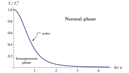
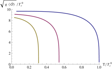
Figure 2: On the left we have the phase diagram of unbalanced holographic superconductor described in the main text. Notice the absence of the Chandrasekhar-Clogston bound (see Figure On the right we have various scalar condensates plotted against temperature. The condensation occurs at lower temperature for increasing values of the chemical imbalance $\delta\mu$.

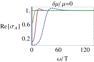
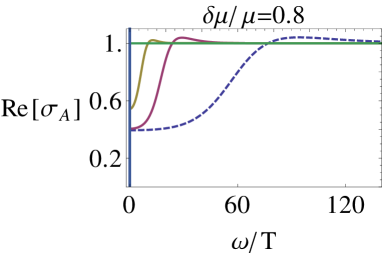
Figure 3: Real part of the optical “electric” conductivity at various temperature $T>T_{c}$ in a balanced (left) and an unbalanced (right) situation. At high temperature we obtain a featureless $\sigma_{A}$ (namely a horizontal line); for lower temperature, instead, a depletion region at low $\omega$ becomes increasingly pronounced. The dashed lines correspond to $T=T_{c}$.

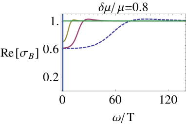
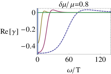
Figure 4: Real part of the “magnetic” and mixed spin-electric conductivities in the normal phase. The dashed line is associated to $T=T_{c}$.

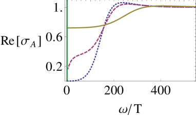
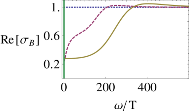
Figure 5: The “electric” and “magnetic” conductivities in the superconducting phase. The features at small values of $\omega$ are due to the interplay of different scales; both $\mu$ and $\delta\mu$ are indeed different from zero.

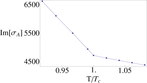
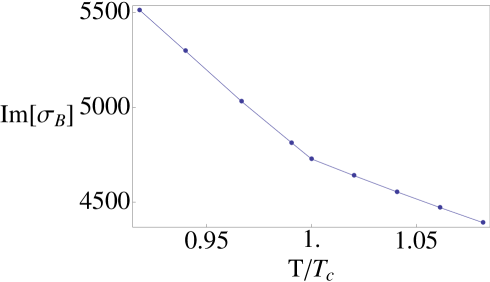
Figure 6: Superconducting/normal state transition associated to a discontinuous behavior of the derivative of the DC conductivity. We have the “electric” and “magnetic” conductivities respectively in the upper and the lower plot. As described in the main text, notice that we have “spin superconductivity” without spin symmetry breaking.

Figure 7: Mixed spin-electric conductivity in the superconducting phase for increasingly lower temperature and fixed chemical imbalance. The dashed plot refers to the conductivity at $T_{c}$.

4 Conclusion

We have here reported some results obtained in [1] where a minimal model for an unbalanced holographic superconductor was introduced and studied. In the present account we have added some new comments and observations especially about the interrelation between the chemical imbalance and the condensation, about the nature of the effective holographic approach to superconductivity and about the time-reversal properties of the system.

The picture emerging at equilibrium shows that the chemical imbalance between the two species (interpreted here as “spin-up” and “spin-down” electrons) hinders the s-wave superconducting condensation; this result matches the weak coupling expectation. Another result we obtained is that our specific model does not manifest any Chandasekar-Clogston bound; this means that, at any value of the chemical imbalance, the system undergoes a superconducting phase transition at sufficiently low temperature. Such a feature emerging in our strongly coupled system is in contrast with the weak-coupling expectation based on a BCS analysis. However, it has to be recognized that equilibrium properties could be quite sensitive to the specific details of the model such as the values of the mass and charge for the scalar field.

The lack of a Chandrasekhar-Clogston bound suggests the absence of a LOFF phase where an inhomogeneous superconducting condensate is thermodynamically favored with respect to a homogeneous one. Such a conclusion is driven by the comparison of the phase diagrams for the unbalanced superconductor at weak coupling, Figure 1, and the phase diagram of our strongly coupled model, Figure 2. In [1] an analytical argument based on an analysis of the unbalanced superconductor in the so-called probe approximation was given to exclude LOFF phases for our minimal model and parameter assignments.

The system at hand is very rich in relation to transport properties and, in particular, it shows interesting mixed features (i.e. effects related to the non-trivial off-diagonal entries in the conductivity matrix). In its normal phase the systems can be regarded as a generalization to strong coupling of the simplest spintronic model (i.e. Mott model [21]). A noteworthy feature is that here the optical conductivity matrix admits a parametrization in terms of a single mobility function $f(\omega)$. This possibility emerges directly from the structure of the equations of motion for the vector fluctuations and its form is suggestively in line with a would-be quasi-particle-like interpretation.

We observed that the mixed spin-electric transport properties of our system are crucially related to the coupling of the fields to the metric; in other words, to study mixed transport one needs to consider the backreaction of the fields on the geometry. As a direct consequence we have that mixed transport phenomena are ubiquitous in holographic systems whenever one consider the full backreacted gravitational system. More generally, let us mention that, as opposed to the equilibrium properties of the system, its transport features are universal and insensitive to the details of the model such as the values of the scalar field parameters.

5 Future perspectives

The present system allows for many generalizations; one among the simplest extensions consists in considering a second scalar field which could serve as an order parameter for the “magnetic” $U(1)$. Such possibility has been already investigated in [16] relying on a probe-approximation analysis. Such extended system is interesting in view of a holographic exploration of the coexistence of different order parameters and their mutual interaction (e.g. competition/enhancement).

The mixed spin-electric conductivity in the superconducting phase shows an interesting enhancement in the low $\omega$ region. In a recent paper, [17], a similar feature has been argued to be possibly related to momentum relaxation and Drude-like behavior. This interesting possibility has to be further investigated and the present model could offer a simple playground on which similar ideas could be tested.

It recently appeared a paper studying angular momentum and spin transport relying on the analysis of the dual bulk spin connection [23]. It would be interesting to understand the relations between their and our approach to address spin transport in a holographic context.

6 Acknowledgements

I am extremely grateful to Francesco Bigazzi, Aldo Cotrone, Alberto Lerda, Davide Forcella, Riccardo Argurio, Johanna Erdmenger, Lorenzo Calibbi, Daniel Arean, Ignacio Salazar Landea, Massimo D’Elia, Carlo Maria Becchi, Alessandro Braggio, Andrea Amoretti, Diego Redigolo, Nicola Maggiore, Nicodemo Magnoli, Katherine Michele Deck and Hongbao Zhang for their useful advices and very interesting conversations. My work was partially supported by the ERC Advanced Grant ”SyDuGraM”, by IISN-Belgium (convention 4.4514.08) and by the “Communauté Française de Belgique” through the ARC program.

References

- [1] F. Bigazzi, A. L. Cotrone, D. Musso, N. P. Fokeeva and D. Seminara, “Unbalanced Holographic Superconductors and Spintronics,” JHEP 1202, 078 (2012) [arXiv:1111.6601 [hep-th]].
- [2] O. Aharony, S. S. Gubser, J. M. Maldacena, H. Ooguri and Y. Oz, “Large N field theories, string theory and gravity,” Phys. Rept. 323, 183 (2000) [hep-th/9905111].
- [3] A. Zaffaroni, “RTN lectures on the non AdS / non CFT correspondence,” PoS RTN 2005, 005 (2005).
- [4] S. S. Gubser, “Breaking an Abelian gauge symmetry near a black hole horizon,” Phys. Rev. D 78, 065034 (2008) [arXiv:0801.2977 [hep-th]].
- [5] S. A. Hartnoll, C. P. Herzog and G. T. Horowitz, “Building a Holographic Superconductor,” Phys. Rev. Lett. 101, 031601 (2008) [arXiv:0803.3295 [hep-th]].
- [6] S. A. Hartnoll, C. P. Herzog and G. T. Horowitz, “Holographic Superconductors,” JHEP 0812, 015 (2008) [arXiv:0810.1563 [hep-th]].
- [7] G. T. Horowitz, “Theory of Superconductivity,” Lect. Notes Phys. 828, 313 (2011) [arXiv:1002.1722 [hep-th]].
- [8] C. P. Herzog, “Lectures on Holographic Superfluidity and Superconductivity,” J. Phys. A 42, 343001 (2009) [arXiv:0904.1975 [hep-th]].
- [9] S. A. Hartnoll, “Lectures on holographic methods for condensed matter physics,” Class. Quant. Grav. 26, 224002 (2009) [arXiv:0903.3246 [hep-th]].
- [10] I. R. Klebanov and E. Witten, “AdS / CFT correspondence and symmetry breaking,” Nucl. Phys. B 556, 89 (1999) [hep-th/9905104].
- [11] D. Musso, “D-branes and Non-Perturbative Quantum Field Theory: Stringy Instantons and Strongly Coupled Spintronics,” arXiv:1210.5600 [hep-th].
- [12] A. I. Larkin and Y. N. Ovchinnikov, “Nonuniform state of superconductors,” Zh. Eksp. Teor. Fiz. 47, 1136 (1964) [Sov. Phys. JETP 20, 762 (1965)]. P. Fulde and R. A. Ferrell, “Superconductivity in a Strong Spin-Exchange Field,” Phys. Rev. 135, A550 (1964).
- [13] R. Casalbuoni and G. Nardulli, “Inhomogeneous superconductivity in condensed matter and QCD,” Rev. Mod. Phys. 76, 263 (2004) [arXiv:hep-ph/0305069].
- [14] B. S. Chandrasekhar, “A note on the maximum critical field of high field superconductors,” Appl. Phys. Lett. 1, 7 (1962). A. M. Clogston, “Upper Limit For The Critical Field In Hard Superconductors,” Phys. Rev. Lett. 9, 266 (1962).
- [15] A. Fert, “Nobel Lecture: Origin, development, and future of spintronics,” Rev. Mod. Phys. 80, 1517 (2008). I. Zutic, J. Fabian and S. Das Sarma, “Spintronics: Fundamentals and applications,” Rev. Mod. Phys. 76, 1323 (2004).
- [16] D. Musso, “Competition/Enhancement of Two Probe Order Parameters in the Unbalanced Holographic Superconductor,” arXiv:1302.7205 [hep-th].
- [17] I. Amado, D. Arean, A. Jimenez-Alba, K. Landsteiner, L. Melgar and I. S. Landea, “Holographic Type II Goldstone bosons,” arXiv:1302.5641 [hep-th].
- [18] S. Weinberg, “Superconductivity For Particular Theorists,” Prog. Theor. Phys. Suppl. 86, 43 (1986).
- [19] J. P. Gauntlett, J. Sonner and T. Wiseman, “Quantum Criticality and Holographic Superconductors in M-theory,” JHEP 1002 (2010) 060 [arXiv:0912.0512 [hep-th]].
- [20] N. Bobev, A. Kundu, K. Pilch and N. P. Warner, “Minimal Holographic Superconductors from Maximal Supergravity,” JHEP 1203 (2012) 064 [arXiv:1110.3454 [hep-th]].
- [21] N. F. Mott, “The electrical Conductivity of Transition Metals,” Proc. R. Soc. Lond. A 153, 699 (1936). “The Resistance and Thermoelectric Properties of the Transition Metals,” Proc. R. Soc. Lond. A 156, 368 (1936).
- [22] J. Erdmenger, V. Grass, P. Kerner and T. H. Ngo, “Holographic Superfluidity in Imbalanced Mixtures,” JHEP 1108, 037 (2011) [arXiv:1103.4145 [hep-th]].
- [23] K. Hashimoto, N. Iizuka and T. Kimura, “Towards Holographic Spintronics,” arXiv:1304.3126 [hep-th].