Three–dimensional brittle fracture:
configurational-force-driven crack propagation

Abstract

This paper presents a computational framework for quasi-static brittle fracture in three dimensional solids. The paper set outs the theoretical basis for determining the initiation and direction of propagating cracks based on the concept of configurational mechanics, consistent with Griffith’s theory. Resolution of the propagating crack by the finite element mesh is achieved by restricting cracks to element faces and adapting the mesh to align it with the predicted crack direction. A local mesh improvement procedure is developed to maximise mesh quality in order to improve both accuracy and solution robustness and to remove the influence of the initial mesh on the direction of propagating cracks. An arc-length control technique is derived to enable the dissipative load path to be traced. A hierarchical hp-refinement strategy is implemented in order to improve both the approximation of displacements and crack geometry. The performance of this modelling approach is demonstrated on two numerical examples that qualitatively illustrate its ability to predict complex crack paths. All problems are three-dimensional, including a torsion problem that results in the accurate prediction of a doubly-curved crack.

1 Introduction

Fracture is a pervasive problem in materials and structures and predictive modelling of crack propagation remains one of the most significant challenges in solid mechanics. A computational framework for modelling crack propagation must not only be able to predict the initiation and the direction of cracks but also to provide a numerical setting to accurately resolve the crack path.

In the Finite Element Method, strategies for discretization of the discontinuities can be categorized as either smeared or discrete. The former is attractive from the point of view that the problem can be solved within a continuum setting, without the need for approximation of discontinuities or changing mesh connectivity. However, as strains localize, numerical difficulties arise and regularization is required. Discrete approaches are able to directly approximate macroscopic crack geometry and therefore describe fractures in a more natural and straightforward manner in terms of displacement jumps and tractions. Developments include introducing embedded displacement jumps within finite elements via additional enhanced strain modes (for example [1]) or with enrichment functions in the context of the partition of unity (PoU) method, e.g. [2].

A straightforward discrete crack approach is to restrict the crack path to element faces. In the simplest case, the predicted path can be strongly influenced by the mesh, thereby influencing the crack surface area, and strongly affecting the amount of energy dissipated. The crack path’s dependence on the mesh can be somewhat reduced by using very fine, unstructured meshes, but this results in computationally expensive analyses. It is worth noting that the authors [3, 4] have shown that within a cohesive crack methodology applied to heterogeneous microstructures, the crack propagation is largely controlled by the need for the mesh to resolve the heterogeneities. However, in the modelling of ideally brittle homogeneous materials, studied here, this is clearly not the case.

In addition to the need for the mesh to resolve the crack, it is necessary to employ some rational means of determining if a crack will propagate and, if so, the direction of crack propagation. The approach taken in this paper is based on the principle of maximal energy dissipation, using configurational forces to determine the direction of the propagating crack front. A similar technique was successfully adopted by a number of authors, but here we mainly follow the work of Miehe and colleagues [5, 6].

This paper is primarily concerned with predicting crack propagation in large three-dimensional problems. The efficiency of such problems, with a large number of degrees of freedom, usually requires the use of an iterative solver for solving the system of algebraic equations. In this case, it is important to control element quality in order to optimise the system matrix conditioning, thereby increasing the computational efficiency of the solver. This can be problematic in methods such as PoU, where the enrichment functions not only the increases the bandwidth of the stiffness matrix but also the matrix conditioning deteriorates [24]. In this paper we will show how controlling the mesh quality improves both the crack path predictions and the robustness of the solution algorithm. Local r-adaptivity is adopted to mitigate the influence of the mesh.

Two numerical examples for crack propagation are presented that demonstrate the ability of the formulation to accurately predict crack paths without bias from the underlying mesh and the influence of mesh adaptivity and mesh quality control on the solution obtained.

2 Body and crack kinematics

Continuous evolution of propagating cracks are analysed within the context of the Arbitrary Lagrangian Eulerian description. This is expressed by differentiable mappings from the reference material configuration to both the current spatial configuration and the current material configuration. In the context of this paper, these mappings are utilized to independently observe the deformation of material in the physical space $\Omega_{t}$ and the evolution of the crack surface in the material space $\mathscr{B}_{t}$, see Fig. 1.

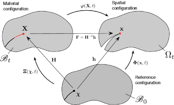
Figure 1: Deformation and structural change of a body with a propagating crack.

The material coordinates $\mathbf{X}$ are mapped onto the spatial coordinates $\mathbf{x}$ via the familiar deformation map $\boldsymbol{\varphi}$, so that

$${\boldsymbol{\varphi}}:\mathscr{B}_{t}\to\Omega_{t},\,\mathbf{x}={\boldsymbol{\varphi}}(\mathbf{X},t)$$ (1)

The mapping ${\boldsymbol{\varphi}}$ must be differentiable, injective, and orientation preserving except at the boundary. The physical displacements are:

$$\mathbf{u}=\mathbf{x}-\mathbf{X}$$ (2)

The reference configuration describes the body before crack extension, with mapping ${\boldsymbol{\Xi}}$ of the reference coordinates $\boldsymbol{\chi}$ on to the material coordinates $\mathbf{X}$ as:

$${\boldsymbol{\Xi}}:\mathscr{B}_{0}\to\mathscr{B}_{t},\,\mathbf{X}={\boldsymbol{\Xi}}(\boldsymbol{\chi},t)$$ (3)

This mapping represents a material structural change, which, in the context of this work, is an extension of the crack due to movement of the crack front. We can also define a mapping ${\boldsymbol{\Phi}}$ of the reference coordinates on to the spatial coordinates as:

$${\boldsymbol{\Phi}}:\mathscr{B}_{0}\to\Omega_{t},\,\mathbf{x}={\boldsymbol{\Phi}}(\boldsymbol{\chi},t)$$ (4)

For convenience, we define a composite space-time vector containing both a coordinate vector and time. For example:

$$(\boldsymbol{\chi},t)=(\chi_{1},\chi_{2},\chi_{3},t)$$ (5)

Thus, the following derivatives can be expressed as

$$\frac{\partial\{{\boldsymbol{\Xi}}(\boldsymbol{\chi},t),t\}}{\partial(\boldsymbol{\chi},t)}=\left[\begin{array}[]{cc}\frac{\partial\boldsymbol{\Xi}}{\partial\boldsymbol{\chi}}&\frac{\partial\boldsymbol{\Xi}}{\partial t}\\[5.0pt] \mathbf{0}^{\textrm{T}}&1\end{array}\right]=\left[\begin{array}[]{cc}\mathbf{H}&\dot{\mathbf{W}}\\[5.0pt] \mathbf{0}^{\textrm{T}}&1\end{array}\right]$$ (6)

$$\frac{\partial\{{\boldsymbol{\Phi}}(\boldsymbol{\chi},t),t\}}{\partial(\boldsymbol{\chi},t)}=\left[\begin{array}[]{cc}\frac{\partial\boldsymbol{\Phi}}{\partial\boldsymbol{\chi}}&\frac{\partial\boldsymbol{\Phi}}{\partial t}\\[5.0pt] \mathbf{0}^{\textrm{T}}&1\end{array}\right]=\left[\begin{array}[]{cc}\mathbf{h}&\dot{\mathbf{w}}\\[5.0pt] \mathbf{0}^{\textrm{T}}&1\end{array}\right]$$ (7)

where the material and spatial displacement fields are

$$\mathbf{W}=\mathbf{X}-{\boldsymbol{\chi}}\quad\textrm{and}\quad\mathbf{w}=\mathbf{x}-{\boldsymbol{\chi}}$$ (8)

$\mathbf{H}$ and $\mathbf{h}$ are the gradients of the material and spatial maps. Given the inverse of (6) as

$$\left({\frac{\partial\{{\boldsymbol{\Xi}}(\boldsymbol{\chi},t),t\}}{\partial(\boldsymbol{\chi},t)}}\right)^{-1}=\left[\begin{array}[]{cc}\mathbf{H}&\dot{\mathbf{W}}\\ \mathbf{0}^{\textrm{T}}&1\end{array}\right]^{-1}=\left[\begin{array}[]{cc}\mathbf{H}^{-1}&-\mathbf{H}^{-1}\dot{\mathbf{W}}\\ \mathbf{0}^{\textrm{T}}&1\end{array}\right]$$ (9)

then

$$\frac{\partial\{{\boldsymbol{\varphi}}(\mathbf{X},t),t\}}{\partial(\mathbf{X},t)}=\left(\frac{\partial\{{\boldsymbol{\Phi}}(\boldsymbol{\chi},t),t\}}{\partial(\boldsymbol{\chi},t)}\right)\,\left({\frac{\partial\{{\boldsymbol{\Xi}}(\boldsymbol{\chi},t),t\}}{\partial(\boldsymbol{\chi},t)}}\right)^{-1}=\left[\begin{array}[]{cc}\mathbf{h}\mathbf{H}^{-1}&\dot{\mathbf{w}}-\mathbf{h}\mathbf{H}^{-1}\dot{\mathbf{W}}\\ \mathbf{0}^{\textrm{T}}&1\end{array}\right]$$ (10)

It can be seen from (10) that the deformation gradient is

$$\mathbf{F}=\frac{\partial\boldsymbol{\varphi}}{\partial\mathbf{X}}=\mathbf{h}\mathbf{H}^{-1}$$ (11)

Given that the physical material cannot penetrate itself or reverse the orientation of material coordinates, we have:

$$\textrm{det}(\mathbf{F})=\frac{\textrm{det}(\mathbf{h})}{\textrm{det}(\mathbf{H})}>0$$ (12)

In addition, from Eq. (10), we can define the velocity of a material point $\mathbf{X}$ and the time derivative of the deformation gradient of a point $\mathbf{X}=\textrm{const}$ as

$$\dot{\mathbf{u}}=\dot{\boldsymbol{\varphi}}=\dot{\mathbf{w}}-\mathbf{h}\mathbf{H}^{-1}\dot{\mathbf{W}}=\dot{\mathbf{w}}-\mathbf{F}\dot{\mathbf{W}}$$ (13)

and

$$\dot{\mathbf{F}}=\nabla_{\mathbf{X}}\dot{\mathbf{w}}-\mathbf{h}\mathbf{H}^{-1}\nabla_{\mathbf{X}}\dot{\mathbf{W}}$$ (14)

3 Crack, crack front and boundary conditions in material space

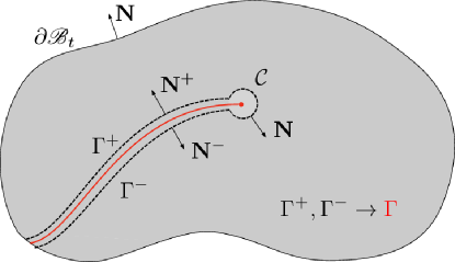
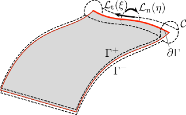
Figure 2: Crack construction.

Similar to [6], the crack surface is denoted as $\Gamma\in\mathscr{B}_{t}$, with a crack front $\partial\Gamma$. The two faces of the crack surface are given by $\Gamma^{+}$ and $\Gamma^{-}$ and $\mathcal{C}$ is a surface that encircles the crack front, see Figure 2. The crack surface is obtained by the limits $\Gamma^{+},\Gamma^{-}\to\Gamma$ and $|\mathcal{C}|\to 0$. The surface $\Gamma$ in three dimensional space can be parameterized by coordinates $\xi$ and $\eta$, such that $\Gamma=\Gamma(\xi,\eta)$. Defining $\mathbf{T}^{+,-}_{\xi}$ and $\mathbf{T}^{+,-}_{\eta}$ as the tangent vectors to the surface $\Gamma^{+,-}$:

$$\mathbf{T}^{+,-}_{\xi}=\left.\frac{\partial\Gamma^{+,-}(\xi,\eta)}{\partial\xi}\right|_{\eta=\textrm{const}}\quad\textrm{and}\quad\mathbf{T}^{+,-}_{\eta}=\left.\frac{\partial\Gamma^{+,-}(\xi,\eta)}{\partial\eta}\right|_{\xi=\textrm{const}}$$ (15)

the crack normal vectors $\mathbf{N}^{+,-}$ to the surfaces $\Gamma^{+,-}$ are then given as

$$\mathbf{N}^{+,-}=\mathbf{\mathbf{T}^{+,-}_{\xi}}\times\mathbf{T}^{+,-}_{\eta}=\textrm{Spin}[\mathbf{T}^{+,-}_{\xi}]\mathbf{T}^{+,-}_{\eta}$$ (16)

The $\textrm{Spin}[\cdot]$ operator is introduced for convenience in calculating derivatives.

The crack surface area is given as:

$$A_{\Gamma}=\frac{1}{2}(A^{+}_{\Gamma}+A^{-}_{\Gamma})=\frac{1}{2}\sum_{i}^{+,-}\int_{\Gamma^{i}}\|\mathbf{N}^{i}\|\textrm{d}\xi\textrm{d}\eta$$ (17)

The change of this crack surface area in the material configuration, for continuously evolving surfaces $\Gamma^{+}$ and $\Gamma^{-}$, is expressed as

$$\begin{split}\dot{A}_{\Gamma}&=\frac{1}{2}\sum^{+,-}_{i}\int_{\Gamma^{i}}\left\{\frac{\mathbf{N}^{i}}{\|\mathbf{N}^{i}\|}\cdot\left(\textrm{Spin}\left[\mathbf{T}^{i}_{\xi}\right]\frac{\partial\mathbf{T}^{i}_{\eta}}{\partial\mathbf{W}}-\textrm{Spin}\left[\mathbf{T}^{i}_{\eta}\right]\frac{\partial\mathbf{T}^{i}_{\xi}}{\partial\mathbf{W}}\right)\right\}\dot{\mathbf{W}}\textrm{d}\xi\textrm{d}\eta\\ &=\frac{1}{2}\sum^{+,-}_{i}\int_{\Gamma^{i}}\mathbf{A}_{\Gamma^{i}}\cdot\dot{\mathbf{W}}\textrm{d}S\end{split}$$ (18)

where, in the limit, $\mathbf{A}_{\Gamma^{+}},\mathbf{A}_{\Gamma^{-}}\to\mathbf{A}_{\Gamma}$. This quantity describes the current orientation of the crack surface. The evolution of $\mathbf{A}_{\Gamma}$ is driven by physical considerations discussed in the following sections. It should be noted that $\mathbf{A}_{\Gamma}$ is a well defined vector for every point on the surface $\Gamma$, including the crack front $\partial\Gamma$, and has dimensions of $m^{-1}$.

The surface encircling the crack front $\mathcal{C}$ can be parameterised by two families of curves, see Figure 2, $\mathcal{L}(\xi)_{\textrm{t}}=\mathcal{C}(\xi,\eta)|_{\eta=\textrm{const}}$ and $\mathcal{L}(\eta)_{\textrm{n}}=\mathcal{C}(\xi,\eta)|_{\xi=\textrm{const}}$. In the limit $|\mathcal{C}|\to 0$ and integrals over the crack front are given by

$$\lim_{|\mathcal{C}|\to 0}\int_{\mathcal{C}}(\cdot)\textrm{d}S:=\lim_{|\mathcal{C}|\to 0}\int_{\mathcal{L}_{\textrm{t}}}\int_{\mathcal{L}_{\textrm{n}}}(\cdot)\textrm{d}S=\int_{\partial\Gamma}\lim_{|\mathcal{L}_{\textrm{n}}|\to 0}\int_{\mathcal{L}_{\textrm{n}}}(\cdot)\textrm{d}S.$$ (19)

The surface $\Gamma$ is created by a curve $\mathcal{L}_{\textrm{t}}(\xi)$ that is swept along the path which is determined by the direction of $\mathbf{A}_{\Gamma}$. The kinematic relationship between the crack surface area $A_{\Gamma}$ and the crack front velocity $\dot{\mathbf{W}}$ on $\mathcal{C}$ is given as

$$\dot{A}_{\Gamma}=\int_{\partial\Gamma}\lim_{|\mathcal{L}_{\textrm{n}}|\to 0}\int_{\mathcal{L}_{\textrm{n}}}\mathbf{A}_{\Gamma}\cdot\dot{\mathbf{W}}\textrm{d}S=\int_{\partial\Gamma}\mathbf{A}_{\partial\Gamma}\cdot\dot{\mathbf{W}}\textrm{d}L.$$ (20)

where $\mathbf{A}_{\partial\Gamma}$ is a kinematic state variable that defines the direction of crack propagation. Note that the spatial velocity field $\dot{\mathbf{w}}$ is restricted in the usual manner by the Dirichlet boundary conditions and interpenetration of surfaces $\Gamma^{+}$ and $\Gamma^{-}$ is not admissible.

4 Dissipation of energy at crack front

We consider a thermodynamic system composed of a solid elastic body with a crack. Forces applied on the boundary of the elastic body $\partial\mathscr{B}_{t}$ can do work on the system and all energy within the volume of the body can be used to do mechanical work. Exchange of energy between the crack surface and the exterior is restricted to the crack front. No free energy is stored at the crack front to do mechanical work on the elastic body. Making use of Eq. (13), the power of external work on the elastic body is given as:

$$\mathscr{P}:=\int_{\partial\mathscr{B}_{t}}\dot{\mathbf{u}}\cdot\mathbf{t}\textrm{d}S=\int_{\partial\mathscr{B}_{t}}\left\{\dot{\mathbf{w}}\cdot\mathbf{t}-\dot{\mathbf{W}}\cdot\mathbf{F}^{\textrm{T}}\mathbf{t}\right\}dS$$ (21)

where $\mathbf{t}$ is the external traction vector. The rate of change of internal energy of the system can be decomposed as follows:

$$\dot{\mathscr{U}}:=\dot{\mathscr{U}}_{\Gamma}+\dot{\mathscr{U}}_{\mathscr{B}_{t}}$$ (22)

where $\mathscr{U}_{\Gamma}$ is the internal crack energy and $\mathscr{U}_{\mathscr{B}_{t}}$ is the internal body energy. The former is defined as:

$$\mathscr{U}_{\Gamma}:=\gamma A_{\Gamma}$$ (23)

where $\gamma$ is the surface energy and has dimension $[Nm^{-1}]$. Since the new crack surface is created by the sweep of the curve $\mathcal{L}_{\textrm{t}}$ along the path defined by $\mathbf{A}_{\partial\Gamma}$, the change of the crack surface internal energy (noting Eq. (20)) is expressed as:

$$\dot{\mathscr{U}}_{\Gamma}:=\frac{\textrm{d}}{\textrm{d}t}\mathscr{U}_{\Gamma_{t}}=\gamma\dot{A}_{\Gamma}=\gamma\int_{\partial\Gamma}\mathbf{A}_{\partial\Gamma}\cdot\dot{\mathbf{W}}\textrm{d}L$$ (24)

Since we assume that there is no dissipation of energy within the volume of the body, the change of internal body energy can be expressed by

$$\dot{\mathscr{U}}_{\mathscr{B}_{t}}:=\frac{\textrm{d}}{\textrm{d}t}\int_{\mathscr{B}_{t}}\hat{\Psi}(\mathbf{F})\textrm{d}V,$$ (25)

where $\hat{\Psi}$ is the specific free energy function. Given the relation in Eq. (14) and that $\textrm{d}\dot{V}=\nabla_{\mathbf{X}}\cdot\dot{\mathbf{W}}\textrm{d}V$, Eq. (25) can be expressed as

$$\dot{\mathscr{U}}_{\mathscr{B}_{t}}=\int_{\mathscr{B}_{t}}\{\mathbf{P}:\nabla_{\mathbf{X}}\dot{\mathbf{w}}+{\boldsymbol{\Sigma}}:\nabla_{\mathbf{X}}\dot{\mathbf{W}}\}\textrm{d}V$$ (26)

where

$$\mathbf{P}:=\frac{\partial\Psi(\mathbf{F})}{\partial\mathbf{F}},\quad{\boldsymbol{\Sigma}}:=\Psi(\mathbf{F})\mathbf{1}-\mathbf{F}^{\textrm{T}}\mathbf{P}$$ (27)

are the first Piola-Kirchhoff stress and Eshelby stress tensors, respectively. Therefore, the first law of thermodynamics, $\mathscr{P}=\dot{\mathscr{U}}_{\Gamma}+\dot{\mathscr{U}}_{\mathscr{B}_{t}}$, can be expressed as

$$\int_{\partial\mathscr{B}_{t}}\left\{\dot{\mathbf{w}}\cdot\mathbf{t}-\dot{\mathbf{W}}\cdot\mathbf{F}^{\textrm{T}}\mathbf{t}\right\}\textrm{d}S=\int_{\partial\Gamma}\gamma\mathbf{A}_{\partial\Gamma}\cdot\dot{\mathbf{W}}\textrm{d}L+\int_{\mathscr{B}_{t}}\{\mathbf{P}:\nabla_{\mathbf{X}}\dot{\mathbf{w}}+{\boldsymbol{\Sigma}}:\nabla_{\mathbf{X}}\dot{\mathbf{W}}\}\textrm{d}V$$ (28)

In order to get a local form of the first law, the Gauss divergence theorem is applied to the last integral in Eq. (28) resulting in the following expression

$$\begin{split}\int_{\partial\Gamma}\gamma\mathbf{A}_{\partial\Gamma}\cdot\dot{\mathbf{W}}\textrm{d}L&=\int_{\mathscr{B}_{t}}\dot{\mathbf{w}}\cdot\{\nabla_{\mathbf{X}}\cdot\mathbf{P}\}\textrm{d}V+\int_{\mathscr{B}_{t}}\dot{\mathbf{W}}\cdot\{\nabla_{\mathbf{X}}\cdot{\boldsymbol{\Sigma}}\}\textrm{d}V\\ &+\int_{\partial\mathscr{B}_{t}\cup\Gamma^{+}\cup\Gamma^{-}}\dot{\mathbf{w}}\cdot\{\mathbf{t}-\mathbf{P}\mathbf{N}\}\textrm{d}S+\int_{\partial\mathscr{B}_{t}\cup\Gamma^{+}\cup\Gamma^{-}}\dot{\mathbf{W}}\cdot\{\mathbf{F}^{\textrm{T}}\mathbf{t}+\boldsymbol{\Sigma}\mathbf{N}\}\textrm{d}S\\ &-\int_{\partial\Gamma}\dot{\mathbf{w}}\cdot\lim_{|\mathcal{L}_{\textrm{n}}|\to 0}\int_{\mathcal{L}_{\textrm{n}}}\mathbf{P}\mathbf{N}\textrm{d}S+\int_{\partial\Gamma}\dot{\mathbf{W}}\cdot\lim_{|\mathcal{L}_{\textrm{n}}|\to 0}\int_{\mathcal{L}_{\textrm{n}}}\boldsymbol{\Sigma}\mathbf{N}\textrm{d}S.\end{split}$$ (29)

The spatial and material conservation laws of linear momentum balance, for any point inside the body, are expressed as:

$$\nabla_{\mathbf{X}}\cdot\mathbf{P}=\mathbf{0},\quad\nabla_{\mathbf{X}}\cdot{\boldsymbol{\Sigma}}=\mathbf{0}$$ (30)

Considering admissible velocity fields and stress fields in equilibrium with external forces, we obtain the following:

$$\int_{\partial\Gamma}\gamma\mathbf{A}_{\partial\Gamma}\cdot\dot{\mathbf{W}}\textrm{d}L-\int_{\partial\Gamma}\dot{\mathbf{W}}\cdot\lim_{|\mathcal{L}_{\textrm{n}}|\to 0}\int_{\mathcal{L}_{\textrm{n}}}\{\boldsymbol{\Sigma}\mathbf{N}\}\textrm{d}S=0$$ (31)

Thus, the local form of the first law is:

$$\dot{\mathbf{W}}\cdot\left(\gamma\mathbf{A}_{\partial\Gamma}-\mathbf{G}_{\partial\Gamma}\right)=0$$ (32)

where the configurational (or material) force at the crack front, that is driving the crack extension, is defined as:

$$\mathbf{G}_{\partial\Gamma}=\lim_{|\mathcal{L}_{\textrm{n}}|\to 0}\int_{\mathcal{L}_{\textrm{n}}}\boldsymbol{\Sigma}\mathbf{N}\textrm{d}L$$ (33)

Eq. (32 ) represents the equilibrium condition for the crack front. One solution is trivial, i.e. that there is no crack growth ($\dot{\mathbf{W}}=\mathbf{0}$); another solution is that $\left(\gamma\mathbf{A}_{\partial\Gamma}-\mathbf{G}_{\partial\Gamma}\right)=\mathbf{0}$; a third solution is that $\dot{\mathbf{W}}$ is orthogonal to $\left(\gamma\mathbf{A}_{\partial\Gamma}-\mathbf{G}_{\partial\Gamma}\right)$. Note that the first law only defines if the crack is in equilibrium but not how it will evolve.

Since the free energy of the elastic body can be transformed into work at the crack front (or other forms of energy) but no energy is stored on the crack surface that can be used to do mechanical work on the body, the local variant of the second law is simply given as:

$$\mathscr{D}:=\gamma\dot{\mathbf{W}}\cdot\mathbf{A}_{\partial\Gamma}\geq 0$$ (34)

where $\mathscr{D}$ is the dissipation of energy per unit length of the crack front and is equivalent to the local change of the crack surface internal energy. This equation expresses the constraint that a physically admissible evolution of the crack is restricted to positive crack area growth at each point of the crack front. Healing is not thermodynamically admissible unless some other (bio/chemo/mechanical) process takes place. Although the second law places restrictions on the direction of crack evolution, it does not determine how $\mathbf{A}_{\partial\Gamma}$ or $\dot{\mathbf{W}}$ evolves and therefore has to be supplemented by a constitutive law; this is described in the next section. With this constitutive law, configurational mechanics provides a thermodynamically consistent framework which accounts for topological changes to the material body, in the form of crack propagation, and delivers the material displacement field $\mathbf{W}$ and the work conjugate configurational forces $\mathbf{G}_{\partial\Gamma}$.

5 Material resistance

A straightforward criterion for crack growth, in the spirit of Griffith, is proposed:

$$\phi(\mathbf{G}_{\partial\Gamma})=\mathbf{G}_{\partial\Gamma}\cdot\mathbf{A}_{\partial\Gamma}-g_{c}/2\leq 0$$ (35)

where $g_{c}$ is is a material parameter specifying the critical threshold of energy release per unit area of the crack surface $\Gamma$.

The principle of maximum dissipation for each point of the crack front states that, for all possible Griffith-like forces $\mathbf{G}^{*}_{\partial\Gamma}$ that satisfy Eq. (35), for a given crack configuration, the dissipation $\mathscr{D}$ attains its maximum for the actual configurational force $\mathbf{G}_{\partial\Gamma}$. Therefore, we have

$$(\mathbf{G}_{\partial\Gamma}-\mathbf{G}^{*}_{\partial\Gamma})\cdot\dot{\mathbf{W}}\geq 0$$ (36)

Using the classical method of Lagrange multipliers, we transform this into an unconstrained minimisation problem. The Lagrangian functional is therefore defined as:

$$\mathscr{L}(\mathbf{G}^{*}_{\partial\Gamma},\dot{\kappa})=-\mathbf{G}^{*}_{\partial\Gamma}\cdot\dot{\mathbf{W}}+\dot{\kappa}\phi(\mathbf{G}^{*}_{\partial\Gamma}).$$ (37)

and the Kuhn-Tucker conditions become

$$\frac{\partial\mathscr{L}}{\partial\mathbf{G}^{*}_{\partial\Gamma}}=-\dot{\mathbf{W}}+\dot{\kappa}\mathbf{A}_{\partial\Gamma}=0,\quad\dot{\kappa}\geq 0,\quad\phi(\mathbf{G}^{*}_{\partial\Gamma})\leq 0,\quad\textrm{and}\quad\dot{\kappa}\phi(\mathbf{G}^{*}_{\partial\Gamma})=0.$$ (38)

In an unloading situation, i.e. $\phi<0$, we get the trivial solution of no crack growth,

$$\dot{\mathbf{W}}=\mathbf{0},$$ (39)

where the first law (28) is automatically satisfied and the crack orientation $\mathbf{A}_{\partial\Gamma}$ is determined by the current crack geometry. For loading of a point at the crack front, $\dot{\kappa}>0$ (and $\phi=0$),

$$\dot{\mathbf{W}}=\dot{\kappa}\mathbf{A}_{\partial\Gamma},$$ (40)

which constrains the crack extension $\dot{\mathbf{W}}$ to be collinear to $\mathbf{A}_{\partial\Gamma}$. Referring back to the first law (Eq. (32)) and the crack growth criterion (Eq. (35)), we therefore have:

$$\gamma\mathbf{A}_{\partial\Gamma}=\mathbf{G}_{\Gamma}\quad\textrm{and}\quad 2\gamma=g_{c}$$ (41)

Applying the principle of maximum dissipation, the crack propagation direction is determined by the configurational force. A thermodynamically admissible crack propagation is only possible for a positive local change of the crack surface area (see Eq. (34). We note that $\dot{\kappa}$ has dimension of length and represents the crack surface kinematic state variable which we can identify as

$$\dot{A}_{\Gamma}\equiv\int_{\partial\Gamma}\dot{\kappa}\,\textrm{d}L\geq 0$$ (42)

This is in agreement with the restriction implied by the second law, Eq. (34). It should be noted that, for simplicity, only an isotropic crack resistance is considered here. However, the current methodology could be easily extended for anisotropic materials.

For a general loading case, the formulation presented could result in unstable crack propagation. Therefore, in this work, the external force is controlled such that the crack surface evolves quasi-statically.

6 Spatial and material discretization

The finite element approximation is applied for both the material and physical space

$$\begin{array}[]{c}\mathbf{X}^{\textrm{h}}={\boldsymbol{\Phi}}(\boldsymbol{\chi})\widetilde{\mathbf{X}},\quad\mathbf{x}^{\textrm{h}}={\boldsymbol{\Phi}}(\boldsymbol{\chi})\widetilde{\mathbf{x}}\\ \mathbf{W}^{\textrm{h}}={\boldsymbol{\Phi}}(\boldsymbol{\chi})\dot{\widetilde{\mathbf{W}}},\quad\mathbf{w}^{\textrm{h}}={\boldsymbol{\Phi}}(\boldsymbol{\chi})\dot{\widetilde{\mathbf{w}}}\end{array}$$ (43)

where superscript h indicates approximation and $\left(\tilde{\cdot}\right)$ indicates nodal values. Three-dimensional domains are discretised with tetrahedral finite elements with hierarchical basis functions of arbitrary polynomial order, following the work of Ainsworth and Coyle [12]. The higher-order approximations are only applied to displacements in the spatial configuration, whereas a linear approximation is used for displacements in the material space. The material and spatial gradients of deformation are expressed in the classical form

$$\mathbf{H}^{\textrm{h}}=\mathbf{B}_{\mathbf{X}}(\boldsymbol{\chi})\widetilde{\mathbf{X}},\quad\mathbf{h}^{\textrm{h}}=\mathbf{B}_{\mathbf{x}}(\boldsymbol{\chi})\widetilde{\mathbf{x}}$$ (44)

and the physical deformation gradient can be expressed as:

$$\mathbf{F^{\textrm{h}}}=\mathbf{h}^{\textrm{h}}(\mathbf{H}^{\textrm{h}})^{-1}=\mathbf{B}_{\mathbf{x}}(\mathbf{X})\widetilde{\mathbf{x}}$$ (45)

6.1 Crack direction

The normal to the discretized crack surface $\Gamma^{\textrm{h}}$, applying the FE approximation, is given by (c.f. Eq (16)):

$$\mathbf{N}^{\textrm{h}}=\textrm{Spin}\left[\frac{\partial\mathbf{X}^{\textrm{h}}}{\partial\xi}\right]\frac{\partial\mathbf{X}^{\textrm{h}}}{\partial\eta}$$ (46)

where $\xi$ and $\eta$ are local coordinates of an element’s triangular face on the crack surface. This normal is constant for a linear element and is easily calculated at Gauss integration points for higher-order approximations. Utilising Eq. (46) and with reference to Eq. (18), the approximation to the change in crack area can be expressed as

$$\begin{split}\dot{A}_{\Gamma}^{\textrm{h}}&=\frac{1}{2}\left\{\operatorname*{\raisebox{-2.0pt}{${{{{{\mathsf{A}}}}}}$}}_{\textrm{TRI}}\int_{\textrm{TRI}}\frac{\mathbf{N}}{\|\mathbf{N}\|}\cdot\left(\textrm{Spin}\left[\frac{\partial\mathbf{X}^{\textrm{h}}}{\partial\xi}\right]\frac{\partial{\boldsymbol{\Phi}}}{\partial\mathbf{\eta}}-\textrm{Spin}\left[\frac{\partial\mathbf{X}^{\textrm{h}}}{\partial\mathbf{\eta}}\right]\frac{\partial{\boldsymbol{\Phi}}}{\partial\xi}\right)\textrm{d}\xi\textrm{d}\eta\right\}\dot{\widetilde{\mathbf{W}}}\\ &=\frac{1}{2}\left\{\operatorname*{\raisebox{-2.0pt}{${{{{{\mathsf{A}}}}}}$}}_{\textrm{TRI}}\int_{\textrm{TRI}}\mathbf{A}^{\textrm{h}}_{\Gamma}\textrm{d}\xi\textrm{d}\eta\right\}\dot{\widetilde{\mathbf{W}}}=\widetilde{\mathbf{A}}^{\textrm{h}}_{\Gamma}\dot{\widetilde{\mathbf{W}}}\end{split}$$ (47)

where $\operatorname*{\raisebox{-2.0pt}{${{{{{\mathsf{A}}}}}}$}}_{\textrm{TRI}}$ indicates the standard FE assembly for the triangular surfaces of elements. The discrete matrix $\widetilde{\mathbf{A}}^{\textrm{h}}_{\Gamma}$ has dimensions of length.

It is important to reiterate that nodes on the discretised crack surface $\Gamma^{\textrm{h}}$ are allowed to move in the material configuration, but the overall body shape and its volume are constant in time. Furthermore, admissible changes in material nodal coordinates cannot change the shape of the crack faces (nor the total area of the crack surface), except for nodes on the crack front $\partial\Gamma^{\textrm{h}}$. As a consequence, the matrix $\widetilde{\mathbf{A}}^{\textrm{h}}_{\Gamma}$ has a number of nonzero rows equal to the number of active crack front nodes. The columns represents the contribution of the unit nodal material velocities ($\dot{\widetilde{\mathbf{W}}}$) to changes of the crack surface area $A^{\textrm{h}}_{\Gamma}$.

Each row of matrix $\widetilde{\mathbf{A}}^{\textrm{h}}_{\Gamma}$ can be interpreted as containing the components of a node’s material velocity which lead to a change of crack area. We can define the vector of nodal Griffith-like forces, which represent material resistance, as

$$\mathbf{f}^{\textrm{h}}_{\textrm{crack,material}}:=\frac{1}{2}\left(\widetilde{\mathbf{A}}^{\textrm{h}}_{\Gamma}\right)^{\textrm{T}}\mathbf{g}_{c}$$ (48)

where $\mathbf{g}_{c}$ is a vector of size equal to the number of nodes, with $g_{c}$ for each component. These nodal Griffith-like forces have dimensions of Newtons $[N]$, which are work conjugate to the material displacement $\mathbf{W}$ on the crack front.

6.2 Residuals in spatial and material space

The residual force vector in the discretised spatial configuration is expressed as:

$$\mathbf{r}^{\textrm{h}}_{\textrm{space}}:=\lambda\mathbf{f}^{\textrm{h}}_{\textrm{ext,space}}-\mathbf{f}^{\textrm{h}}_{\textrm{int,space}}$$ (49)

where $\lambda$ is an the unknown load factor and $\mathbf{f}^{\textrm{h}}_{\textrm{ext,space}}$ and $\mathbf{f}^{\textrm{h}}_{\textrm{int,space}}$ are the vectors of external and internal forces, respectively, and defined as follows

$$\mathbf{f}^{\textrm{h}}_{\textrm{ext,space}}:=\operatorname*{\raisebox{-2.0pt}{${{{{{\mathsf{A}}}}}}$}}_{\textrm{TRI}}\int_{\textrm{TRI}}{\boldsymbol{\Phi}}^{\textrm{T}}\mathbf{t}^{\textrm{h}}_{\lambda}\textrm{d}S,\quad\mathbf{f}^{\textrm{h}}_{\textrm{int,space}}=\operatorname*{\raisebox{-2.0pt}{${{{{{\mathsf{A}}}}}}$}}_{\textrm{TET}}\int_{\textrm{TET}}\left(\mathbf{B}_{\mathbf{x}}\right)^{\textrm{T}}\mathbf{P}^{\textrm{h}}\textrm{d}S$$ (50)

where $\operatorname*{\raisebox{-2.0pt}{${{{{{\mathsf{A}}}}}}$}}_{\textrm{TET}}$ indicates the standard FE assembly for tetrahedral elements. Similarly, the residual vector for nodal degrees of freedom in the material configuration is given by

$$\mathbf{r}^{\textrm{h}}_{\textrm{material}}:=\mathbf{f}^{\textrm{h}}_{\textrm{crack,material}}-\mathbf{f}^{\textrm{h}}_{\textrm{int,material}}$$ (51)

where $\mathbf{f}^{\textrm{h}}_{\textrm{int,material}}$ is the nodal values of configurational forces

$$\mathbf{f}^{\textrm{h}}_{\textrm{int,material}}:=\operatorname*{\raisebox{-2.0pt}{${{{{{\mathsf{A}}}}}}$}}_{\textrm{TET}}\int_{\textrm{TET}}\left(\mathbf{B}_{\mathbf{x}}\right)^{\textrm{T}}{\boldsymbol{\Sigma}}^{\textrm{h}}\textrm{d}S$$ (52)

We note that for a continuous elastic body comprising an homogeneous material, the configurational forces within the volume should be zero. For a discretised homogeneous body, any non-zero values are an indication of a solution error. In [13], this is utilised to improve solution quality by displacing the nodal positions in the material space. However, this improvement methodology is numerically expensive since it introduces large non-linearities into the system which are difficult to tackle in three-dimensional problems and can lead to convergence problems. For this reason, the nodal configurational force vector is calculated only for nodes on the crack front and an alternative approach is adopted to reduce any numerical errors in the vicinity of the crack front. An hp-adaptivity strategy is adopted utilising the hierarchical approximation basis [12] described above and a simple mesh refinement technique, using edge-based subdivision, in the vicinity of the crack front [14].

Calculating the nodal configurational forces only for the nodes at the crack front, we can write

$$(\widetilde{\mathbf{G}}^{\textrm{h}}_{\Gamma})_{I}:=(\mathbf{f}^{\textrm{h}}_{\textrm{int,material}})_{I}\quad\textrm{for}\quad I\in\{I:\mathcal{N}_{I}\,\textrm{is crack front node}\}$$ (53)

Finally, utilising Eq. (48), the material residual Eq. (49) is now expressed as

$$\mathbf{r}^{\textrm{h}}_{\textrm{material}}=\frac{1}{2}\left(\widetilde{\mathbf{A}}_{\Gamma}^{\textrm{h}}\right)^{\textrm{T}}\mathbf{g_{c}}-\widetilde{\mathbf{G}}^{\textrm{h}}_{\Gamma}$$ (54)

6.3 Discrete crack propagation criterion

The crack propagation criterion for a discretised problem is expressed by a scalar product of the material residual and the nodal $\widetilde{\mathbf{A}}_{\Gamma}^{\textrm{h}}$, resulting in

$$\widetilde{\mathbf{\phi}}^{\textrm{h}}:=\widetilde{\mathbf{A}}_{\Gamma}^{\textrm{h}}\mathbf{r}^{\textrm{h}}_{\textrm{material}}=\frac{1}{2}\widetilde{\mathbf{A}}_{\Gamma}^{\textrm{h}}(\widetilde{\mathbf{A}}_{\Gamma}^{\textrm{h}})^{\textrm{T}}\mathbf{g_{c}}-\widetilde{\mathbf{A}}_{\Gamma}^{\textrm{h}}\widetilde{\mathbf{G}}^{\textrm{h}}_{\Gamma}<\mathbf{0},$$ (55)

which can be expressed for each crack front node $I$ as:

$$g_{c}-2\left[\left((\widetilde{\mathbf{A}}^{\textrm{h}}_{\Gamma})^{\textrm{T}}\widetilde{\mathbf{A}}^{\textrm{h}}_{\Gamma}\right)^{-1}\widetilde{\mathbf{A}}^{\textrm{h}}_{\Gamma}\widetilde{\mathbf{G}}^{\textrm{h}}_{\Gamma}\right]_{I}<0$$ (56)

For nodes on the crack front for which the fracture criterion is satisfied, nodes are doubled and selected faces split. Faces are chosen based on the direction of the material force $(\widetilde{\mathbf{G}}^{\textrm{h}}_{\Gamma})_{I}$. A procedure for face splitting is described in the following section.

Eq (56) involves a matrix inversion, where the size of the inverted matrix is equal to the number of nodes on the crack front. A more straightforward alternative is:

$$g_{c}-2\frac{(\widetilde{\mathbf{A}}^{\textrm{h}}_{\Gamma})_{I}(\widetilde{\mathbf{G}}^{\textrm{h}}_{\Gamma})_{I}}{\|(\widetilde{\mathbf{A}}^{\textrm{h}}_{\Gamma})_{I}\|^{2}}<0$$ (57)

This has been tested and no significant difference to Eq (56) was found. Therefore, Eq. (57) is used for all analyses, although a more detailed investigation is needed in the future.

The criteria (56) and (57) are a generalization of that presented by Gürses and Miehe in [6], where, based on dimensional consistency, the magnitude of the configurational nodal force is divided by the average length of the edges adjacent to the node being split:

$$g_{c}-\frac{\|\mathbf{G}_{\Gamma}\|}{L_{\textrm{ave}}}<0.$$ (58)

This latter fracture criterion is equivalent to the one used here (Eq. (57)) only for nodes with two collinear edges.

6.4 Crack Propagation and Arc-length Method

To trace the quasi-static dissipative loading path, we assume that the crack front is in a state of quasi-equilibrium and satisfies the crack propagation criterion Eq. (57), within some tolerance:

$$|g_{c}-2\frac{(\widetilde{\mathbf{A}}^{\textrm{h}}_{\Gamma})_{I}(\widetilde{\mathbf{G}}^{\textrm{h}}_{\Gamma})_{I}}{\|(\widetilde{\mathbf{A}}^{\textrm{h}}_{\Gamma})_{I}\|^{2}}|<\epsilon$$ (59)

where $\epsilon$ is a parameter that depends on the characteristic mesh size. From an equilibrium configuration, the crack front is extended at each node on the crack front by one element length in the direction of the configurational force $\tilde{\mathbf{G}}_{\Gamma}^{\textrm{h}}$. This crack extension is resolved by the FE mesh using an r-adaptivity approach, whereby, for each node on the crack front, associated element faces are realigned with the predicted crack direction and a discontinuity is introduced by splitting the mesh at these faces. This process is repeated for all nodes on the crack front. The methodology for choosing an appropriate face for realignment and for subsequently splitting the mesh differs from that described in [6] and is discussed in Section 8. Inevitably, realignment of element faces will reduce the quality of the elements in the neighbourhood of the crack front, and this is also discussed in Section 8.

For the new configuration, we adapt the external load factor $\lambda$ to achieve global equilibrium using an arc-length technique. Therefore, the system of equations for conservation of the material and spatial momentum is supplemented by a load control equation in the form

$$r_{\lambda}=\mathbf{1}\cdot\widetilde{\mathbf{A}}^{\textrm{h}}_{\Gamma}\widetilde{\mathbf{X}}_{n}-\mathbf{1}\cdot\widetilde{\mathbf{A}}^{\textrm{h}}_{\Gamma}\widetilde{\mathbf{X}}^{i+1}_{n+1}=0,$$ (60)

where all nodal contributions to the crack surface area are added with the use of vector $\mathbf{1}$. This approach of extending the crack and subsequently determining the corresponding load factor means that we can simplify the analysis technique by avoiding the need for developing an algorithm to deal with the non-smooth Kuhn-Tucker loading/unloading conditions, controlling the load such that the quasi-static crack propagation criterion is enforced at each step.

6.5 Linearised system of equations

In the proposed framework, the global equilibrium solution is obtained by the Newton-Raphson method (see Algorithm 1), converging when the norms of residuals $\mathbf{r}_{\textrm{spatial}}$, $\mathbf{r}_{\textrm{material}}$ and $r_{\lambda}$ are less than a given tolerance. This is solved for material and spatial displacements, as a fully coupled problem. We apply a standard linearisation procedure (see for example, [13, 17] for details) to the material $\mathbf{r}^{\textrm{h}}_{\textrm{material}}$ and spatial residuals $\mathbf{r}^{\textrm{h}}_{\textrm{space}}$, resulting in a linear system of equations for iteration $i$ and load step $n+1$:

$$\left[\begin{array}[]{ccc}\partial_{\widetilde{\mathbf{x}}}\mathbf{f}^{\textrm{h}}_{\textrm{int,space}}&\partial_{\widetilde{\mathbf{x}}}\mathbf{r}^{\textrm{h}}_{\textrm{material}}&-\partial_{\widetilde{\mathbf{x}}}\mathbf{f}^{\textrm{h}}_{\textrm{ext,space}}\\ \partial_{\widetilde{\mathbf{X}}}\mathbf{f}^{\textrm{h}}_{\textrm{int,space}}&\partial_{\widetilde{\mathbf{X}}}\mathbf{r}^{\textrm{h}}_{\textrm{material}}&-\partial_{\widetilde{\mathbf{X}}}\mathbf{f}^{\textrm{h}}_{\textrm{ext,space}}\\ \mathbf{0}&\partial_{\widetilde{\mathbf{X}}}r_{\lambda}&0\end{array}\right]\left\{\begin{array}[]{c}\delta\widetilde{\mathbf{x}}^{i+1}\\ \delta\widetilde{\mathbf{X}}^{i+1}\\ \delta\lambda^{i+1}\end{array}\right\}=-\left[\begin{array}[]{l}\mathbf{r}^{\textrm{h}}_{\textrm{space}}\\ \mathbf{r}^{\textrm{h}}_{\textrm{material}}\\ r_{\lambda}\end{array}\right]$$ (61)

where $\widetilde{\mathbf{X}}^{i+1}=\widetilde{\mathbf{X}}^{i}+\delta\widetilde{\mathbf{X}}^{i+1}$, $\widetilde{\mathbf{x}}^{i+1}=\widetilde{\mathbf{x}}^{i}+\delta\widetilde{\mathbf{x}}^{i+1}$ and $\lambda^{i+1}=\lambda^{i}+\delta\lambda^{i+1}$.

Data: Model parameters and problem geometry

initialise load step $n=0$;

while body not fully fractured do

       for all nodes on crack front do

             if crack propagation criterion (57) is violated then

                   extend crack front

             end if

            

       end for

      initialise iteration $i=0$;

       update reference configuration $\mathscr{B}_{0}\leftarrow\mathscr{B}_{t}$;

       while not converged do

             compute tangents and residuals and
solve linearised system of equations (see (61));

             $\widetilde{\mathbf{X}}_{n+1}^{i+1}\leftarrow\widetilde{\mathbf{X}}_{n+1}^{i}+\delta\widetilde{\mathbf{X}}^{i+1}$;

             $\widetilde{\mathbf{x}}_{n+1}^{i+1}\leftarrow\widetilde{\mathbf{x}}_{n+1}^{i}+\delta\widetilde{\mathbf{x}}^{i+1}$;

             $\lambda_{n+1}^{i+1}\leftarrow\lambda_{n+1}^{i+1}+\delta\lambda^{i+1}$;

            

            set iteration $i\leftarrow i+1$;

            

       end while

      

      save data at load step $n$;

       load step $n\leftarrow n+1$;

      

end while

Algorithm 1 Solution procedure

7 Mesh quality control

Extension of the crack front can result in poor quality elements in the vicinity of the crack front, including inverted or severely distorted elements, that can make the problem difficult or impossible to solve. To address this, we apply a similar approach to the one proposed by Scherer et al. [13]. The key challenge is to enforce constraints to preserve element quality for each Newton-Raphson iteration, without influencing the physical response. Thus, we introduce a measure of element quality for tetrahedral elements in terms of their shape and use this to drive mesh improvement. Here we restrict ourselves to movement of nodes, with no changes to element topology. By applying this methodology we are able to solve large problems on parallel computers using Krylov iterative solvers with standard preconditioners.

The dihedral angles formed between the faces of a tetrahedron have been shown to be one of the most influential properties in terms of solution accuracy [25]. Large dihedral angles result in interpolation errors and small dihedral angles affect the conditioning of the stiffness matrix. The minimum sine of the dihedral angles has been used in [25], however, this is a non-smooth function that cannot be used with a Newton-Raphson solver. To overcome this, an alternative volume-length measure is proposed. Although this measure does not directly measure dihedral angles, it has been shown to be very effective at eliminating poor angles, thus improving stiffness matrix conditioning and interpolation errors [15, 16]. As the volume-length measure is a smooth function of vertex positions and its gradient is straightforward and computationally cheap to calculate, it is ideal for the problem at hand. The volume-length quality measure is defined as

$$q(\mathbf{H}^{\textrm{h}}):=6\sqrt{2}\frac{V_{0}}{l_{\textrm{rms},0}^{3}}\frac{\textrm{det}(\mathbf{H}^{\textrm{h}})}{dl_{\textrm{rms}}^{3}(\mathbf{H}^{\textrm{h}})}=q_{0}b(\mathbf{H}^{\textrm{h}}),\quad b(\mathbf{H}^{\textrm{h}}):=\frac{\textrm{det}(\mathbf{H}^{\textrm{h}})}{dl_{\textrm{rms}}^{3}(\mathbf{H}^{\textrm{h}})}$$ (62)

where $q_{0}$, $V_{0}$ and $l_{\textrm{rms},0}$ are the element quality, element volume and root mean square of the element’s edge lengths respectively, in the reference configuration. $\mathbf{H}^{\textrm{h}}$ is the material deformation gradient, $b$ is measure of change of element quality, relative to the reference configuration, and $dl_{\textrm{rms}}=l_{\textrm{rms}}/l_{\textrm{rms},0}$ is the stretch of $l_{\textrm{rms},0}$ from the reference configuration. $q_{0}$ is normalised so that an equilateral element has quality $1$ and a degenerate element (zero volume) has quality $0$. Furthermore, $b=1$ corresponds to no change and $b=0$ is a change leading to a degenerate element. An element edge length in the material configuration is expressed as

$$l_{j}(\mathbf{H}^{\textrm{h}}):=\sqrt{\Delta{\boldsymbol{\chi}}_{j}^{\textrm{T}}(\mathbf{H}^{\textrm{h}})^{\textrm{T}}\mathbf{H}^{\textrm{h}}\Delta{\boldsymbol{\chi}}_{j}}$$ (63)

where $\Delta{\boldsymbol{\chi}}^{j}$ and is the distance vector of edge $j$ in the reference configuration. Thus $l_{\textrm{rms}}$ is calculated as

$$l_{\textrm{rms}}:=\sqrt{\frac{1}{6}\sum_{j=1}^{6}l_{j}^{2}}=l_{\textrm{rms},0}dl_{\textrm{rms}}$$ (64)

To control the quality of elements, we enforce an admissible deformation $\mathbf{H}^{\textrm{h}}$ such that

$$b(\mathbf{H}^{\textrm{h}})>\gamma\quad\textrm{for}\;\gamma\in(0,1)$$ (65)

In practice, $0.1<\gamma<0.5$ gives good results. This constraint on $b$ is enforced by applying a volume–length log–barrier function [13] defined as

$$\mathcal{B}:=\sum_{e=0}^{\mathcal{N}}\frac{b_{e}^{2}}{2(1-\gamma)}-\ln(b_{e}-\gamma)$$ (66)

where $\mathcal{B}$ is the barrier function for the change in element quality in the material configuration. It can be seen that the Log–Barrier function rapidly increases as the quality of an element reduces, and tends to infinity when the quality approaches the barrier $\gamma$, thus achieving our aim of penalising the worst quality elements.

In order to build a solution scheme that incorporates a stabilising force that controls element quality, we define a pseudo ‘stress’ at the element level as a counterpart of the first Piola–Kirchhoff stress as follows

$$\mathbf{Q}:=\frac{\partial\mathcal{B}}{\partial\mathbf{H}^{\textrm{h}}}=\textrm{det}(\mathbf{H}^{\textrm{h}})\frac{l_{\textrm{lrms},0}^{3}}{l_{\textrm{lrms}}^{3}}\left(\frac{b}{1-\gamma}+\frac{1}{b-\gamma}\right)\widetilde{\mathbf{Q}},$$ (67)

where matrix $\widetilde{\mathbf{Q}}$ is defined as follows

$$\widetilde{\mathbf{Q}}:=(\mathbf{H}^{\textrm{h}})^{-\textrm{T}}-\frac{1}{2}\frac{1}{l_{\textrm{lrms}}^{2}}\sum_{j=1}^{6}\Delta{\mathbf{X}}^{j}(\Delta{\boldsymbol{\chi}}^{j})^{\textrm{T}}.$$ (68)

It is worth noting that $\mathbf{Q}$ should be a zero matrix for a purely volumetric change or rigid body movement of a tetrahedral element.

It is now possible to compute a vector of nodal pseudo ‘forces’ associated with $\mathbf{Q}$ as

$$\mathbf{f}^{\textrm{h}}_{\textrm{quality}}=\operatorname*{\raisebox{-2.0pt}{${{{{{\mathsf{A}}}}}}$}}_{\textrm{TET}}\int_{\textrm{TET}}\alpha\mathbf{B}^{\textrm{T}}_{\mathbf{X}}\mathbf{Q}\textrm{d}V$$ (69)

where $\alpha$ is a solution parameter that can vary from $0$ to $1$ but is typically set to $1$. Thus, the global vector of nodal material residual forces (Eq. (51)) is now augmented with this additional stabilisation term $\mathbf{f}^{\textrm{h}}_{\textrm{quality}}$ to give:

$$\mathbf{r}^{\textrm{h}}_{\textrm{material}}:=\mathbf{f}^{\textrm{h}}_{\textrm{crack,material}}-\mathbf{f}^{\textrm{h}}_{\textrm{int,material}}+\mathbf{f}^{\textrm{h}}_{\textrm{quality}}$$ (70)

Starting from an equilibrium state (i.e. configurational forces and griffith-like forces are equal and the arc-length control (Eq. (60)) is satisfied), a subsequent load step will generally result in a loss of equilibrium and mesh deformation will occur, with changes in element quality controlled by the volume–length log–barrier function. Thus, for any arbitrary perturbation from equlibrium, by $\delta\widetilde{\mathbf{X}}$, $\delta\widetilde{\mathbf{x}}$ or $\delta\lambda$, equilibrium would be recovered by the Newton-Raphson procedure irrespective of $\alpha$. However, if $\alpha=0$, there is no control of element quality. In future, it is possible for $\alpha$ to also reflect the magnitude of the out-of-balance material force, providing a damping effect where the current iteration is a long way from equilibrium. To date, this has not been required.

8 Determination of critical faces and mesh realignment

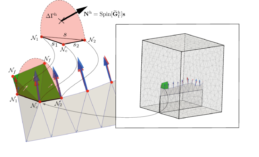
Figure 3: Crack front extension. Green element faces represent admissible crack extension before projection on predicted crack surface extension $\Delta\Gamma^{\textrm{h}}$. Blue arrows represent nodal configurational forces and red arrows represent nodal Griffith-like forces.

To determine which element face will be aligned with the predicted crack front extension and then split in order to create the crack extension, first all nodes on the current crack front are ordered according to the degree with which they violate the discrete crack propagation criterion (57). Taking each of these nodes in turn, we consider a vector $\mathbf{s}=\mathbf{s}_{1}+\mathbf{s}_{2}$ on the crack front associated with node $\mathcal{N}_{c}$, as shown in Fig. 3. Next, the normal of the new crack extension, $\Delta\Gamma^{\textrm{h}}$, is determined as follows:

$$\mathbf{N}^{\textrm{h}}=\textrm{Spin}[\widetilde{\mathbf{G}}^{\textrm{h}}_{\Gamma}]\mathbf{s}$$ (71)

As an example, Fig. 3 illustrates three faces associated with node $\mathcal{N}_{c}$ as well as the predicted crack surface $\Delta\Gamma^{\textrm{h}}$ defined by $\mathbf{N}^{\textrm{h}}$. It is important to emphasise that, in general, there will be more than one admissible set of faces that are associated with node $\mathcal{N}_{c}$, but for simplicity only one set is highlighted in Fig. 3. Only edges and faces which are connected directly to node $\mathcal{N}_{c}$ are considered. Edges and faces which are part of the body’s surface or the existing crack surface are excluded from these considerations as the crack can only propagate in the volume of the body.

For each admissible set of faces, ‘free’ nodes $\mathcal{N}_{f}$ can be identified that can be moved so that the faces are aligned with the predicted crack extension $\Delta\Gamma^{\textrm{h}}$. Each admissible set of faces is tested and that set which results in the least worse element quality (Eq. (62)) is aligned with $\Delta\Gamma^{\textrm{h}}$, nodes are duplicated and the faces are split. The last part of the process is mesh smoothing in the vicinity of the crack front, utilising the methodology described previously.

In the authors’ implementation, the above methodology is achieved by constructing an undirected graph tree for all admissible crack surface extensions for each each node $\mathcal{N}_{c}$. The vertices of the tree represent element edges and lines of the tree represent element faces. The starting vertex is edge $s_{1}$ and the last vertex is edge $s_{2}$. In the case that node $\mathcal{N}_{c}$ is on the surface of the body, it is only associated with one edge, i.e. $\mathbf{s}=\mathbf{s}_{1}$ and the last vertex of the tree can be any edge on the body surface connected to node $\mathcal{N}_{c}$. Each path through the tree represents a possible set of faces that can be realigned and split to form the crack extension.

Once the tree is built, a search over all branches is carried out, i.e. all possible paths which link the two adjacent crack front edges are searched for the set of faces that, when aligned with the predicted crack extension $\Delta\Gamma^{\textrm{h}}$, lead to the least worse quality element (using the volume–length quality measure (Eq. 62)). Thus, this approach is optimal in minimising any possible deterioration in mesh quality as a result of mesh realignment.

Following realignment of the element faces, node $\mathcal{N}_{c}$ and the selected element faces are doubled, creating two new surfaces for the crack extension. Next, mesh smoothing is undertaken for a patch of elements in the vicinity of node $\mathcal{N}_{c}$ utilising the volume-length log-barrier function described in Section 7 to ensure mesh quality. This has been found to be computationally efficient and in practice its execution takes an insignificant fraction of the total solution time. This process was found to be very robust and works well for meshes with varying element size and/or with initially poor quality. It is also worth noting that this procedure of crack extension and mesh smoothing could be implemented in virtually any FE system as an isolated and autonomous procedure since it does not involve any enrichment nor does it change mesh connectivity and only involves doubling of nodes and element faces.

9 Implementation and Numerical Examples

All problems are discretised using 3D tetrahedral elements. An adaptive mesh refinement strategy is adopted that includes both h-refinement, using an edge-based splitting algorithm [14], and p-refinement using hierarchic basis functions identified above [12]. First, all elements $\mathcal{E}_{1}$ adjacent to the crack front are selected, then a larger set of elements $\mathcal{E}_{2}$ adjacent to and including set $\mathcal{E}_{1}$ are selected. All elements in set $\mathcal{E}_{2}$ are subject to edge-based splitting. The spatial nodal positions are discretised using higher-order approximations in the vicinity of the crack front. The spatial nodal positions in all elements in $\mathcal{E}_{2}\backslash\mathcal{E}_{1}$ are discretised using second-order approximation functions and elements in $\mathcal{E}_{1}$ using third-order. This refinement strategy is automated so that the mesh is locally refined while the crack is propagating. This is illustrated in Fig 4. As the crack front moves forward, elements are removed from set $\mathcal{E}_{2}$ and elements revert to their original state.

The solution strategy presented in this paper is implemented for parallel shared memory computers, utilising open-source libraries. MOAB, a mesh-oriented database [18], is used to store mesh data, including input and output operations and information about mesh topology. PETSc (Portable, Extensible Toolkit for Scientific Computation [19]) is used for parallel matrix and vector operations, the solution of linear system of equations and other algebraic operations. ParMetis [20] is used for parallel mesh partitioning, using the PETSc native interface.

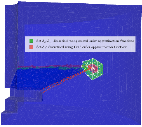
Figure 4: hp-refinement at crack front

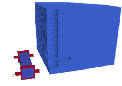
Figure 5: Geometry and relative size comparison for torsion and pull-out test

To demonstrate the proposed modelling framework, two numerical examples are presented: torsion test and pull-out test. For both examples, a quasi-brittle material is considered, i.e. concrete. The torsion test represents the analysis of a relatively small physical sample whereas the pull-out test represents a much larger problem, see Fig. 5. These two tests not only provide a means of verifying the numerical robustness of the presented methodology but also to illustrate the limits of the Griffith-like fracture theory adopted in this paper.

9.1 Pull out test

This problem considers the pull-out of a steel anchor embedded in a concrete cylindrical block, which is surrounded by a steel ring. The problem was simulated by Duan & Areias, Belytschko [8, 9] and Gasser & Holzapfel [10]. All geometrical data has been obtained from [8, 9, 10]. Young’s modulus $E=30000\,\textrm{N/mm}^{2}$, Poison ratio $\nu=0.2$ and Griffith energy $G_{f}=0.106\,\textrm{N/mm}$. Following [8], the anchor itself is not explicitly modelled; instead a uniform prescribed vertical displacement is applied to the concrete face corresponding to the upper face of the anchor’s plate. Only one quarter of the specimen is modelled.

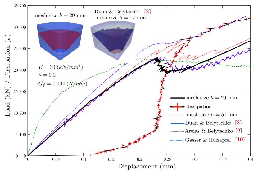
Figure 6: Load-displacement path and energy dissipation for pull-out problem

A coarse mesh comprising $2995$ nodes, with a characteristic mesh size of $51$mm, and a fine mesh comprising $14075$ nodes, with a mesh size of $29$mm, have been used in the analyses. A neo-Hookean material was used initially, but both displacements and strains were found to be small and there was no noticeable difference compared to the solution assuming a linear elastic material was observed. Therefore, all results presented here are for a linear elastic material.

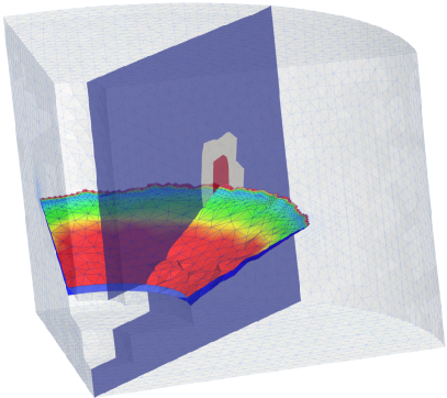
(a)                  (b)

Figure 7: (a) Propagating crack with contour plot on crack surface of strain energy density and contour plot on vertical slice of polynomial order (blue: linear, white: quadratic, red: cubic). (b) Final crack surface. Follow this link for animation of the results for this problem.

Fig. 6 shows the load-displacement response for the two different discretisations. The coarse mesh analysis was undertaken without any mesh refinement at the crack front, whereas the fine mesh analysis included hp-refinement as described earlier. It can be seen that in the latter case, the oscillations in the response are smaller in magnitude.

Fig. 6, also compares the load-displacement paths for simulations of the same problem reported by Gasser & Holzapfel [10], Areias & Belytschko [9] and Duan & Belytschko [8]. All these simulations utilise a cohesive crack methodology together with enrichment functions to approximate displacement discontinuities. The cohesive crack methodology assumes that significant energy is dissipated in the fracture process zone, in the vicinity of the crack front, associated with meso-scale cracking and incorporated into the model by a fictitious extension of the crack front with cohesive forces. The work of these cohesive forces is equal to the work dissipated in the fracture process zone. In cohesive models, energy is dissipated by crack opening; in contrast, in the present work, it is assumed that energy is exclusively dissipated in the process of creating new crack area. The present approach is justified by the assumption that the volume of the fracture process zone (where meso-cracking takes place) is significantly smaller than the total volume of the body and so it can be assumed that energy dissipation is restricted to the crack front (note that aggregates are approximately two orders of magnitude smaller than the diameter of the specimen). This explains the good correlation of the present results with those presented by Duan & Belytschko, see Fig. 6.

It is useful to observe that, in the case of Gasser & Holzapfel [10], the peak strength matches the results of Duan & Belytschko. In the case of Areias & Belytschko [9], the results show an over prediction of strength compared to all other results. It is important to recall that the present model is based only on three material parameters, i.e. two for the elastic solid and the third is the Griffith energy release rate; no additional crack separation law is needed. In spite of this limited number of material parameters, good agreement with the other results is achieved.

9.2 Torsion test

An experimental study by Brokenshire [23] of a torsion test of a plain concrete notched prismatic beam ($400\textrm{mm}\times 100\textrm{mm}\times 100\textrm{mm}$) is considered. The experimental procedure and full details of the boundary conditions and dimensions are described in Jefferson et al. [22]. The notch is placed at an oblique angle across the beam and extends to half the depth. The beam is placed in a steel loading frame, supported at three corners and loaded at the fourth corner. The experiment used aggregates with a maximum size of $10$ mm; the characteristic size of the specimen can be considered to be $100\textrm{mm}$.

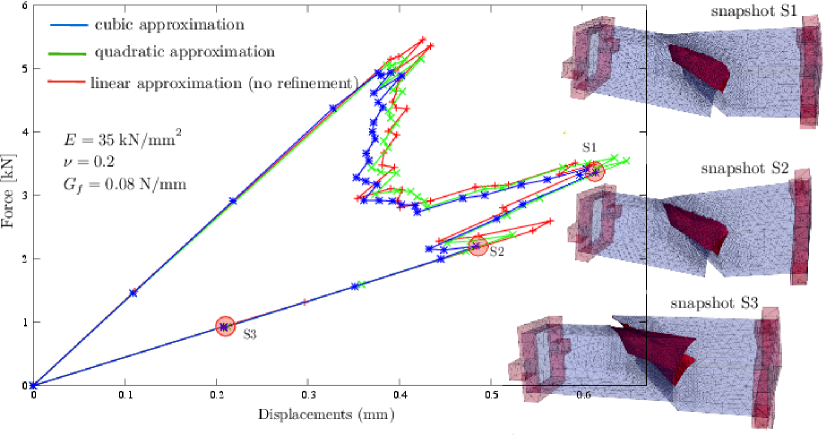
Figure 8: Load-displacement path. Animation for this test is available under this link.

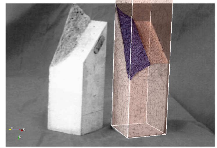
Figure 9: The simulated crack surface superimposed on experimental result  [22].

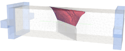
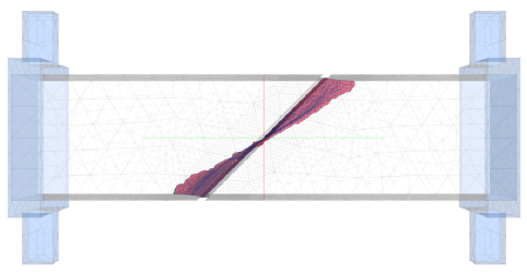
Figure 10: The simulated crack surface viewed from the side and above.

The beam and steel frame are discretized using tetrahedral elements. The mesh consists of $29941$ nodes, see Fig. 8. For this problem, three numerical tests with the same initial mesh are investigated. The first test was without adaptive mesh refinement near the crack front, the second with one level of mesh refinement and a quadratic approximation basis near the crack front and the third with two levels of h-refinement and a cubic hierarchical approximation basis near the crack front. In order to study the rate of convergence associated with refinement, the propagating crack is resolved by splitting the original mesh before refinement (note that in the pull-out test it was the refined mesh that was split). Hence, the mesh refinement improves the approximation quality of the displacements fields, but the resolution of the crack front geometry is the same for all three tests.

Fig. 8 shows the load-displacement response for the three numerical tests. Good numerical convergence is observed with increasing refinement and the arc-length control method is able to track the dissipative loading path. Fig. 9 shows the numerically predicted geometry of the cracked specimen overlain on to the experimentally observed geometry, demonstrating excellent agreement. Despite the good qualitative predictions, the numerical analyses (Fig. 8) over predict the experimental ultimate load by approximately $2.5$ times. This observed difference is a consequence of assuming linear elastic fracture mechanics for a problem where the size of the fracture process zone is significant compared to the size of the problem. This was not an issue in the pull-out test, since the characteristic size of the problem was significantly larger (see Fig. 5). The fracture energy is not only used in the creation of the macroscopic crack surface, but a significant proportion is used to create meso-cracks in the vicinity of the crack front (Bažant [22]). Even though the crack geometry matches the experimental results very well, see Fig. 9, the macro-crack has insufficient surface area to match the total amount of dissipated energy. Dissipation of energy in the macro-cracks is not included in the constitutive model and the meso-cracks are not discretised. An enhancement of the constitutive model to include cohesive cracking is an option for future work.

10 Conclusions

This paper has presented a computational model for quasi-static, three-dimensional, brittle fracture based on configurational mechanics. The model predicts the direction of crack extension based on the principle of energy minimization in conjunction with a node-based Griffith-like crack criterion. The direction of the crack extension is aligned with the nodal configurational forces at the crack front and the crack extension is resolved by locally aligning element faces and then splitting the mesh. Both h- and p-refinement are utilised in the vicinity of the crack front to increase the accuracy of the evolving crack front geometry and the approximation of the spatial displacements. A monolithic solution strategy, simultaneously solving for both the material displacements (i.e. crack extension) and the spatial displacements, is presented. In order to track the dissipative loading path for the ideally brittle material, an arc-length procedure has been derived that is tailored for this model.

A key element of the solution strategy is the control of mesh quality for the evolving problem. A pseudo ‘stress’ for the mesh quality measure is derived as a function of the material gradient of deformation. This mesh quality control is used locally in the vicinity of the crack front following realignment of element faces but it is also used globally to stabilise the Newthon–Raphson method. It is worth noting that this mesh smoothing method could be implemented in any standard FE system using the pseudo ‘stress’, standard shape functions and standard procedures for numerical integration and vector and matrix assembly. A method of selecting the tetrahedral element faces for crack surface approximation is presented. This method is based on an undirected graph (tree) allowing for efficient and robust search among admissible sets of the element faces for crack extension, which leads to minimal mesh distortion.

This formulation can be extended to include the case of anisotropic materials, material heterogeneity and other dissipative processes, for example to capture nonlinear size effect, when the characteristic size of the microstructure needs to be included in the model. To achieve this, thermodynamic constraints on the local state variables can be derived by applying the Coleman procedure [7]. This could potentially allow the model to be extended to include dissipative processes related to crack opening, applying the cohesive crack methodology [3, 4]. In such a situation, the energy dissipation associated with a macroscopic crack and dissipation related to meso-level cracking are quantified independently.

The model has been implemented on parallel shared memory computers using libraries such as PETSc [18] and MOAB [19]. The two numerical examples demonstrated the model’s ability to accurately simulate complex crack paths and to trace the dissipative load-displacement path.

References

- [1] J. Oliver, Modelling strong discontinuities in solid mechanics via strain softening constitutive equations. part 1: fundamentals, International Journal for Numerical Methods in Engineering, 39(21), 3575-3600, 1996.
- [2] G. Wells, Discontinuous modelling of strain localisation and failure, PhD thesis, Technische Universiteit Delft, 2001.
- [3] Ł. Kaczmarczyk, C.J. Pearce, A corotational hybrid-Trefftz stress formulation for modelling cohesive cracks, Computer Methods in Applied Mechanics and Engineering, 198, 1298-1310, 2009.
- [4] Ł. Kaczmarczyk, C.J. Pearce, N. Bićanić, E. de Souza Neto, Numerical multi-scale solution strategy for fracturing heterogeneous materials, Computer Methods in Applied Mechanics and Engineering, 199, 1100-1113, 2010.
- [5] C. Miehe, E. Gürses, M. Birkle,A computational framework of configurational-force-driven brittle fracture propagation based on incremental energy minimization, International Journal of Fracture, 145, 245-259, 2007.
- [6] E. Gürses, C. Miehe, A computational framework of three-dimensional configurational-force-driven brittle crack propagation, Computer Methods in Applied Mechanics and Engineering, 198, 1413-1428, 2009.
- [7] B.D. Coleman and W. Noll. The thermodynamics of elastic materials with heat conduction and viscosity. Arch. Ration. Mech. Anal., 13:167-178, 1963.
- [8] Q. Duan, J.H. Song, T. Menouillard and T. Belytschko, Element-local level set method for three-dimensional dynamic crack growth, International Journal for Numerical Methods in Engineering, 80, 1520-1543, 2009.
- [9] P.M.A. Areias, T. Belytschko, Analysis of three-dimensional crack initiation and propagation using the extended finite element method. International Journal for Numerical Methods in Engineering 2005; 63:760-788.
- [10] T.C. Gasser, G.A. Holzapfel, Modeling 3D crack propagation in unreinforced concrete using PUFEM. Computer Methods in Applied Mechanics and Engineering 2005; 194(25-26):2859-2896.
- [11] A.D. Jeffersonm B.I.G Barr, T. Bennett and S.C. Hee, Three dimensional finite element simulation of fracture test using Craft concrete, Computers and Concrete, 1:3. 261-284, 2004.
- [12] M.A. Ainsworth and J. Coyle, Hierarchic finite element bases on unstructured tetrahedral meshes, International Journal for Numerical Methods in Engineering, International Journal for Numerical Methods in Engineering, 58:14. 2103–2130, 2003.
- [13] M. Scherer, R. Denzer, P. Steinmann, On a solution strategy for energy-based mesh optimization in finite hyperelastostatics, Computer Methods in Applied Mechanics and Engineering. 197 (2008) 609-622.
- [14] D. Ruprecht, H. Müller, A scheme for edge-based adaptive tetrahedron subdivision, Mathematical Visualization, 1994
- [15] J.R. Shewchuk. What Is a Good Linear Finite Element? Interpolation, Conditioning, Anisotropy, and Quality Measures. 2002.
- [16] B. Klingner.Tetrahedral mesh Improvement. PhD thesis, University of California at Berkeley, November 2008.
- [17] E. Kuhl, H. Askes, P. Steinmann, An ALE formulation based on spatial and material settings of continuum mechanics Part 1: Generic hyperelastic formulation, Computer Methods in Applied Mechanics and Engineering, 193 207-4222, 2004.
- [18] S. Balay and J. Brown and K. Buschelman and W.D. Gropp and D. Kaushik and M.G. Knepley and L.C. McInnes and B.F. Smith and H. Zhang, PETSc Web page, http://www.mcs.anl.gov/petsc, 2012.
- [19] Timothy J. Tautges Ray Meyers, Karl Merkley, Clint Stimpson, Corey Ernst, MOAB: A MESH-ORIENTED DATABASE, Sandia Report, Sandia National Laboratories, 2004.
- [20] R. Bender, P. Klinkenberg, Z. Jiang, B. Bauer, G. Karypis, N. Nguyen, M. Perera, B. Nikolau, and C. Carter. Flora: Morphology, Distribution, Function Genomics of Nectar Production in Brassicaceae, Functional Ecology of Plants Volume 207, Issue 7, pp. 491-496, 2012.
- [21] Z. P. Bažant. Size effect on structural strength: a review, Archive of Applied Mechanics 69 703-725, 1999.
- [22] A.D. Jefferson, B.I.G Barr, T. Bennett and S.C. Hee, Three dimensional finite element simulation of fracture test using Craft concrete model, Computers and Concrete, Volume 1, No. 3 261-284, 2004.
- [23] D.R. Brokenshire, A Study of Torsion Fracture Tests, Ph.D. Thesis, Cardiff University, 1996.
- [24] A. Menk, S.P. A. Bordas, A robust preconditioning technique for the extended finite element method, International Journal for Numerical Methods in Engineering Volume 85, Issue 13, pages 1609-1632, 1 April 2011.
- [25] Tian Zhou and Kenji Shimada, An Angle-Based Approach To Two-Dimensional Mesh Smoothing, Proceedings of the 9th international meshing roundtable, 2000.