An Eulerian space-time finite element method for diffusion problems on evolving surfaces

Abstract

In this paper, we study numerical methods for the solution of partial differential equations on evolving surfaces. The evolving hypersurface in $\mathbb{R}^{d}$ defines a $d$-dimensional space-time manifold in the space-time continuum $\mathbb{R}^{d+1}$. We derive and analyze a variational formulation for a class of diffusion problems on the space-time manifold. For this variational formulation new well-posedness and stability results are derived. The analysis is based on an inf-sup condition and involves some natural, but non-standard, (anisotropic) function spaces. Based on this formulation a discrete in time variational formulation is introduced that is very suitable as a starting point for a discontinuous Galerkin (DG) space-time finite element discretization. This DG space-time method is explained and results of numerical experiments are presented that illustrate its properties.

1 Introduction

Partial differential equations (PDEs) posed on evolving surfaces arise in many applications. In fluid dynamics, the concentration of surface active agents attached to an interface between two phases of immiscible fluids is governed by a transport-diffusion equation on the interface [13]. Another example is the diffusion of trans-membrane receptors in the membrane of a deforming and moving cell, which is typically modeled by a parabolic PDE posed on an evolving surface [2].

Recently, several approaches for solving PDEs on evolving surfaces numerically have been introduced. The finite element method of Dziuk and Elliott [6] is based on the Lagrangian description of a surface evolution and benefits from a special invariance property of test functions along material trajectories. If one considers the Eulerian description of a surface evolution, e.g., based on the level set method [19], then the surface is usually defined implicitly. In this case, regular surface triangulations and material trajectories of points on the surface are not easily available. Hence, Eulerian numerical techniques for the discretization of PDEs on surfaces have been studied in the literature. In [1, 21] numerical approaches were introduced that are based on extensions of PDEs off a two-dimensional surface to a three-dimensional neighbourhood of the surface. Then one can apply a standard finite element or (as was done in [1, 21]) finite difference disretization to treat the extended equation in $\mathbb{R}^{3}$. The extension, however, leads to degenerate parabolic PDEs and requires the solution of equations in a higher dimensional domain. For a detailed discussion of this extension approach we refer to [12, 7, 3]. A related approach was developed in  [8], where advection-diffusion equations are numerically solved on evolving diffuse interfaces.

A different Eulerian technique for the numerical solution of an elliptic PDE posed on a hypersurface in $\mathbb{R}^{3}$ was introduced in [17, 15]. The main idea of this method is to use finite element spaces that are induced by the volume triangulations (tetrahedral decompositions) of a bulk domain in order to discretize a partial differential equation on the embedded surface. This method does not use an extension of the surface partial differential equation. It is instead based on a restriction (trace) of the outer finite element spaces to the (approximated) surface. This leads to discrete problems for which the number of degrees of freedom corresponds to the two-dimensional nature of the surface problem, similar to the Lagrangian approach. At the same time, the method is essentially Eulerian as the surface is not tracked by a surface mesh and may be defined implicitly as the zero level of a level set function. For the discretization of the PDE on the surface, this zero level then has to be reconstructed. Optimal discretization error bounds were proved in [17]. The approach was further developed in [4, 18], where adaptive and streamline diffusion variants of this surface finite element were introduced and analysed. These papers [17, 15, 4, 18], however, treated elliptic and parabolic equations on stationary surfaces.

The goal of this paper is to extend the approach from [17] to parabolic equations on evolving surfaces. An evolving surface defines a three-dimensional space-time manifold in the space-time continuum $\mathbb{R}^{4}$. The surface finite element method that we introduce is based on the traces of outer space-time finite element functions on this manifold. The finite element functions are piecewise polynomials with respect to a volume mesh, consisting of four-dimensional prisms (4D prism = 3D tetrahedron $\times$ time interval). For this discretization technique, it is natural to start with a variational formulation of the differential problem on the space-time manifold. To our knowledge such a formulation has not been studied in the literature, yet. One new result of this paper is the derivation and analysis of a variational formulation for a class of diffusion problems on the space-time manifold. For this formulation we prove well-posedness and stability results. The analysis is based on an inf-sup condition and involves some natural, but non-standard, anisotropic function spaces. A second important result is the formulation and analysis of a discrete in time variational formulation that is very suitable as a starting point for a discontinuous Galerkin space-time finite element discretization. Further, we present a finite element method, which then results in discretization (in space and time) of a parabolic equation on an evolving surface.

The discretization approach based on traces of an outer space-time finite element space studied here is also investigated in the recent report [10]. In [10] there is no analysis of the corresponding continuous variational formulation, which is the main topic of this paper. On the other hand, in [10] one finds more information on implementation aspects and an extensive numerical study of properties (accuracy and stability) of this method and some of its variants. Further results of numerical experiments for the example of surfactant transport over two colliding spheres can be found in [11]. We only very briefly comment on implementation aspects and illustrate accuracy and stability properties of the discretization method by results of a few numerical experiments.

In this paper, we do not study discretization error bounds for the presented Eulerian space-time finite element method. This is a topic of current research, first results of which are presented in the follow-up report [16].

The remainder of the paper is organized as follows. In Section 2 we review surface transport-diffusion equations and introduce a space-time weak formulation. Some required results for surface functional spaces are proved in Section 3. A general space-time variational formulation and corresponding well-posedness results are presented in Section 4. A semi-discrete in time method is analyzed in Section 5. A fully discrete space-time finite element method is considered in Section 6. Section 7 contains results of some numerical experiments.

2 Diffusion equation on an evolving surface

Consider a surface $\Gamma(t)$ passively advected by a velocity field $\mathbf{w}=\mathbf{w}(x,t)$, i.e. the normal velocity of $\Gamma(t)$ is given by $\mathbf{w}\cdot\mathbf{n}$, with $\mathbf{n}$ the unit normal on $\Gamma(t)$. We assume that for all $t\in[0,T]$, $\Gamma(t)$ is a smooth hypersurface that is closed ($\partial\Gamma=\emptyset$), connected, oriented, and contained in a fixed domain $\Omega\subset\mathbb{R}^{3}$. To describe the smoothness assumption concerning $\Gamma(t)$ and its evolution more precisely, we introduce the Langrangian mapping from the space-time cylinder $\Gamma_{0}\times[0,T]$, with $\Gamma_{0}:=\Gamma(0)$, to the space-time manifold

$$\mathcal{S}:=\bigcup\limits_{t\in(0,T)}\Gamma(t)\times\{t\},\quad\mathcal{S}\subset\mathbb{R}^{4},$$

see also [8]. We assume that the velocity field $\mathbf{w}$ and $\Gamma_{0}$ are sufficiently smooth such that for all $y\in\Gamma_{0}$ the ODE system

$$\Phi(y,0)=y,\quad\frac{\partial\Phi}{\partial t}(y,t)=\mathbf{w}(\Phi(y,t),t),\quad t\in[0,T],$$

has a unique solution $x:=\Phi(y,t)\in\Gamma(t)$ (recall that $\Gamma(t)$ is transported with the velocity field $\mathbf{w}$). The corresponding inverse mapping is given by $\Phi^{-1}(x,t):=y\in\Gamma_{0}$, $x\in\Gamma(t)$. The Lagrangian mapping $\Phi$ induces a bijection

$$F:\,\Gamma_{0}\times[0,T]\to\mathcal{S},\quad~{}F(y,t):=(\Phi(y,t),t).$$ (1)

We assume this bijection to be a $C^{2}$-diffeomorphism between these manifolds. The conservation of a scalar quantity $u:\mathcal{S}\to\mathbb{R}$ with a diffusive flux on $\Gamma(t)$ leads to the surface PDE (cf. [14]):

$$\dot{u}+({\mathop{\rm div}}_{\Gamma}\mathbf{w})u-{\nu_{d}}\Delta_{\Gamma}u=0\qquad\text{on}~{}~{}\Gamma(t),~{}~{}t\in(0,T],$$ (2)

with initial condition $u(x,0)=u_{0}(x)$ for $x\in\Gamma(0)$. Here

$$\dot{u}=\frac{\partial u}{\partial t}+\mathbf{w}\cdot\nabla u$$

denotes the advective material derivative, ${\mathop{\rm div}}_{\Gamma}:=\operatorname{tr}\left((I-\mathbf{n}\mathbf{n}^{T})\nabla\right)$ is the surface divergence and $\Delta_{\Gamma}$ is the Laplace-Beltrami operator, $\nu_{d}>0$ is the constant diffusion coefficient. Let $H^{1}(\mathcal{S})$ be the usual Sobolev space on $\mathcal{S}$. The following weak formulation of (2) was shown to be well-posed in [6]: Find $u\in H^{1}(\mathcal{S})$ such that $u(\cdot,0)=u_{0}$ and for almost all $t\in(0,T]$

$$\int_{\Gamma(t)}\dot{u}v+uv\,{\mathop{\rm div}}_{\Gamma}\mathbf{w}+\nu_{d}\nabla_{\Gamma}u\cdot\nabla_{\Gamma}v\,ds=0\quad\text{for all}~{}v(\cdot,t)\in H^{1}\big{(}\Gamma(t)\big{)}.$$ (3)

Here $\nabla_{\Gamma}$ is the tangential gradient for $\Gamma(t)$. A similar weak formulation is considered in [20]. The formulation (3) is a natural starting point for the Lagrangian type finite element methods treated in [6, 20]. It is, however, less suitable for the Eulerian finite element method that we introduce in this paper. Our discretization method uses the framework of space-time finite element methods. Therefore, it is natural to consider a space-time weak formulation of (2) as given below. We introduce the space

$$H=\{\,v\in L^{2}(\mathcal{S})~{}|~{}\|\nabla_{\Gamma}v\|_{L^{2}(\mathcal{S})}<\infty\,\}$$

endowed with the scalar product

$$(u,v)_{H}=(u,v)_{L^{2}(\mathcal{S})}+(\nabla_{\Gamma}u,\nabla_{\Gamma}v)_{L^{2}(\mathcal{S})},$$ (4)

and consider the material derivative as a linear functional on $H$. The subspace of all functions $v$ from $H$ such that $\dot{v}$ defines a bounded linear functional form the trial space $W$. A precise definition of the space $W$ is given in Section 3.2. We consider the following weak formulation of (2): Find $u\in W$ such that

$$\begin{split}\left\langle\dot{u},v\right\rangle+\int_{0}^{T}\int_{\Gamma(t)}uv\,{\mathop{\rm div}}_{\Gamma}\mathbf{w}+{\nu_{d}}\nabla_{\Gamma}u\cdot\nabla_{\Gamma}v\,dsdt&=0\qquad\text{for all}~{}v\in H,\\ u(\cdot,0)&=u_{0}.\end{split}$$ (5)

We shall derive certain density properties for the spaces $W$ and $H$, which we need for proving the well-posedness of (5). Actually, we show well-posedness of a slightly more general problem, which includes a possibly nonzero source term and, instead of $({\mathop{\rm div}}_{\Gamma}\mathbf{w})u$, a generic zero order term. Our finite element method will be based on (5) rather than (3).

3 Preliminaries

In this section, we define the trial space $W$ and prove that both the test space $H$ and the trial space $W$ are Hilbert spaces, and that smooth functions are dense in $H$ and $W$. We also prove that a function from $W$ has a well-defined trace as an element of $L^{2}(\Gamma(t))$ for all $[0,T]$. In the setting of a space-time manifold, the spaces $H$ and $W$ are natural ones. In the literature, however, we did not find any analysis of their properties. The necessary results are established with the help of a homeomorphisms between $H$, $W$ and the following standard Bochner spaces $\widehat{H}$ and $\widehat{W}$:

$$\widehat{H}:=L^{2}(0,T;H^{1}(\Gamma_{0})),\qquad\widehat{W}:=\{\,u\in\widehat{H}~{}|~{}\frac{\partial u}{\partial t}\in\widehat{H}^{\prime}\,\},\qquad\Gamma_{0}:=\Gamma(0).$$ (6)

In the next subsection, we collect a few properties of the Bochner spaces $\widehat{H}$ and $\widehat{W}$ that we need in our analysis.

3.1 Properties of the spaces $\widehat{H}$ and $\widehat{W}$

The spaces $\widehat{H}$ and $\widehat{W}$ are endowed with the norms

$$\|u\|_{\widehat{H}}=\left(\int_{0}^{T}\|u(t)\|_{H^{1}(\Gamma_{0})}^{2}\,dt\right)^{\frac{1}{2}}\quad\text{and}\quad\|u\|_{\widehat{W}}=\left(\|u\|_{\widehat{H}}^{2}+\left\|\frac{\partial u}{\partial t}\right\|_{\widehat{H}^{\prime}}^{2}\right)^{\frac{1}{2}}.$$

We start with the following well-known result.

Lemma 1.

The space $C_{0}^{\infty}(\Gamma_{0}\times(0,T))$ is dense in $\widehat{H}$.

Proof.

The inclusion $C_{0}^{\infty}(\Gamma\times(0,T))\subset\widehat{H}$ is trivial. By construction of the Bochner space, the set of simple functions $\left\{\,\sum_{i=1}^{n}\chi_{B_{i}}\phi_{i}~{}|~{}\phi_{i}\in H^{1}(\Gamma_{0}),~{}~{}n\in\mathbb{N}\,\right\}$ is dense in $\widehat{H}$; here $\{B_{i}\}$ is any set of $n$ mutually disjoint measurable subsets of $(0,T)$. For $\chi_{B_{i}}\phi_{i}$ there exists $g_{i}\in C_{0}^{\infty}(0,T)$ and $\widehat{\phi}_{i}\in C^{\infty}(\Gamma_{0})$ such that $\|\chi_{B_{i}}\phi_{i}-g_{i}\widehat{\phi}_{i}\|_{\widehat{H}}$ is arbitrary small. This completes the proof. ∎

For $w\in\widehat{H}$ we define the weak time derivative through the functional

$$\left\langle\frac{\partial w}{\partial t},\phi\right\rangle:=-\int_{0}^{T}\int_{\Gamma_{0}}w(t)\frac{\partial\phi}{\partial t}\,ds\,dt\quad\text{for}~{}~{}\phi\in C^{1}_{0}(\Gamma_{0}\times(0,T)).$$ (7)

Then $\frac{\partial w}{\partial t}\in\widehat{H}^{\prime}$ iff there is a constant $c$ such that

$$\left|\left\langle\frac{\partial w}{\partial t},\phi\right\rangle\right|\leq c\|\phi\|_{\widehat{H}}\quad\text{for all}~{}~{}\phi\in C^{1}_{0}(\Gamma_{0}\times(0,T)).$$

Remark 3.1.

The definition of $\widehat{W}$ in (6), based on the weak time derivative (7), is equivalent to the following more standard one: $w\in\widehat{H}$ is an element of $\widehat{W}$ iff there exists $z\in L^{2}(0,T;H^{-1}(\Gamma_{0}))$ such that

$$\int_{0}^{T}\left\langle z(t),v\right\rangle_{H^{-1}\times H^{1}}\phi(t)\,dt=-\int_{0}^{T}\int_{\Gamma_{0}}w(t)v\phi^{\prime}(t)\,ds\,dt$$ (8)

for all $v\in H^{1}(\Gamma_{0}),~{}\phi\in C_{0}^{\infty}(0,T)$. The definition of $\widehat{W}$ in (6) is more convenient for the analysis that follows.

We recall a few results for the space $\widehat{W}$.

Lemma 2.

The set

$$\mathcal{C}=\left\{\,\sum_{i=1}^{n}t^{i}\phi_{i}~{}|~{}\phi_{i}\in C^{\infty}(\Gamma_{0}),~{}~{}n\in\mathbb{N}\,\right\}$$

is dense in $\widehat{W}$. For $u\in\widehat{W}$ the function $t\to u(t)=u(\cdot,t)$ is continuous from $[0,T]$ into $L^{2}(\Gamma_{0})$. There is a constant $c$ such that

$$\max_{0\leq t\leq T}\|u(t)\|_{L^{2}(\Gamma_{0})}\leq c\|u\|_{\widehat{W}}\quad\text{for all}~{}~{}u\in\widehat{W}.$$ (9)

Proof.

Proofs are given in standard textbooks, e.g., [22] Proposition 23.23. The density result is usually proved with $C^{\infty}(\Gamma_{0})$ replaced by $H^{1}(\Gamma_{0})$ in the definition of $\mathcal{C}$. The result with $C^{\infty}(\Gamma_{0})$ follows from the density of $C^{\infty}(\Gamma_{0})$ in $H^{1}(\Gamma_{0})$. ∎

3.2 The spaces $H$ and $W$

We assume that the space-time surface $\mathcal{S}$ is sufficiently smooth, cf. Section 2. Due to the identity

$$\int_{0}^{T}\int_{\Gamma(t)}f(s,t)\,ds\,dt=\int_{\mathcal{S}}f(\sigma)(1+(\mathbf{w}\cdot\mathbf{n})^{2})^{-\frac{1}{2}}\,d\sigma,$$ (10)

the scalar product $\int_{0}^{T}\int_{\Gamma(t)}vw\,ds\,dt$ induces a norm that is equivalent to the standard norm on $L^{2}(\mathcal{S})$. Therefore, one can equivalently define the norm on $H$ by

$$\|v\|_{H}^{2}:=\int_{0}^{T}\int_{\Gamma(t)}v^{2}+|\nabla_{\Gamma}v|^{2}ds\,dt.$$ (11)

The space $H$ is a Hilbert space, and $H\hookrightarrow L^{2}(\mathcal{S})\hookrightarrow H^{\prime}$ forms a Gelfand triple (cf. Lemma 5 below).

Recall the Leibniz formula

$$\int_{\Gamma(t)}\dot{v}+v{\,\operatorname{div_{\Gamma}}}\mathbf{w}\,ds=\frac{d}{dt}\int_{\Gamma(t)}v\,ds,\quad v\in C^{1}(\mathcal{S}),$$ (12)

which implies the integration by parts identity:

$$\begin{split}&\int_{0}^{T}\int_{\Gamma(T)}\dot{u}v+\dot{v}u+uv{\,\operatorname{div_{\Gamma}}}\mathbf{w}\,ds\,dt\\ &=\int_{\Gamma(T)}u(s,T)v(s,T)\,ds-\int_{\Gamma(0)}u(s,0)v(s,0)\,ds\quad\text{for all}~{}u,v\in C^{1}(\mathcal{S}).\end{split}$$ (13)

Based on (13) we define the material derivative for $u\in H$ as the functional $\dot{u}$:

$$\left\langle\dot{u},\phi\right\rangle=-\int_{0}^{T}\int_{\Gamma(t)}u\dot{\phi}+u\phi{\,\operatorname{div_{\Gamma}}}\mathbf{w}\,ds\,dt\quad\text{for all}~{}~{}\phi\in C_{0}^{1}(\mathcal{S}).$$ (14)

Assume that for some $u\in H$ the norm

$$\|\dot{u}\|_{H^{\prime}}=\sup_{\phi\in C_{0}^{1}(\mathcal{S})}\frac{\left\langle\dot{u},\phi\right\rangle}{\|\phi\|_{H}}$$

is bounded. In Lemma 5 we prove that $C_{0}^{1}(\mathcal{S})$ is dense in $H$ and therefore $\dot{u}$ can be extended to a bounded linear functional on $H$. In this case, we write $\dot{u}\in H^{\prime}$ and define the space

$$W=\{\,u\in H~{}|~{}\dot{u}\in H^{\prime}\,\},\quad\text{with}~{}~{}\|u\|_{W}^{2}:=\|u\|_{H}^{2}+\|\dot{u}\|_{H^{\prime}}^{2}.$$

In Section 3.4 we prove that $W$ is a Hilbert space and $C^{1}(\mathcal{S})$ is dense in $W$. Note that the space $W$ is larger than the standard Sobolev space $H^{1}(\mathcal{S})$. Spaces similar to $H$ and $W$ are introduced and analyzed in [20]. A difference between our aproach and the one used in that paper is that we define $H$ and $W$ directly on the space-time manifold $\mathcal{S}$, whereas in [20] these are defined using a pull back operator to the manifold $\Gamma_{0}\times[0,T]$. We use such a pull back operator in the analysis of the spaces $H$ and $W$ in the next section, but not in their definition.

Remark 3.2.

From the definition of the weak material derivative in (14) and the density result of Lemma 5 it follows that for $u\in C^{1}(\mathcal{S})$ we have

$$\langle\dot{u},v\rangle=\int_{0}^{T}\int_{\Gamma(t)}\dot{u}v\,ds\,dt\quad\text{for all}~{}~{}v\in H.$$

3.3 Homeomorphism between {$\widehat{H}$, $\widehat{W}$} and {$H$, $W$}

Based on the $C^{2}$-diffeomorphism $F$ in (1), for a function $u$ defined on $\mathcal{S}$ we define $\widehat{u}=u\circ F$ on $\Gamma_{0}\times(0,T)$:

$$\widehat{u}(y,t)=u(\Phi(y,t),t)=u(x,t).$$

Vice versa, for a function $\widehat{u}$ defined on $\Gamma_{0}\times(0,T)$ we define $u=\widehat{u}\circ F^{-1}$ on $\mathcal{S}$:

$$u(x,t)=\widehat{u}(\Phi^{-1}(x,t),t)=\widehat{u}(y,t).$$ (15)

By construction we have

$$\dot{u}(x,t)=\frac{\partial\widehat{u}}{\partial t}(y,t).$$ (16)

Now we prove that the mapping $\widehat{u}\to u$ defines a linear homeomorphism between $\widehat{H}$ and $H$, and also between $\widehat{W}$ and $W$.

Lemma 3.

The linear mapping $\widehat{u}\to u$ from (15) defines a homeomorphism between $\widehat{H}$ and $H$.

Proof.

For any fixed $t\in(0,T)$, we obtain $\widehat{u}(t):=\widehat{u}(\cdot,t)\in H^{1}(\Gamma_{0})$ iff $u(t)=u(\cdot,t)\in H^{1}(\Gamma(t))$. Let $\widehat{u}(t)\in H^{1}(\Gamma_{0})$ for all $t\in(0,T)$. Due to the smoothness assumptions on $F$, there are constants $c_{1},c_{0}>0$, independent of $\widehat{u}$ and $t$, such that

$$c_{0}\|\widehat{u}(t)\|_{H^{1}(\Gamma_{0})}\leq\|u(t)\|_{H^{1}(\Gamma(t))}\leq c_{1}\|\widehat{u}(t)\|_{H^{1}(\Gamma_{0})}\quad\text{for all}~{}~{}t\in(0,T).$$ (17)

Hence, $\widehat{u}\in\widehat{H}$ iff $u\in H$ holds, and the linear mapping $\widehat{u}\to u$ is a homeomorphism between $\widehat{H}$ and $H$. ∎

For the further analysis, we need a surface integral transformation formula. For this we consider a local parametrization of $\Gamma_{0}$, denoted by $\mu:\mathbb{R}^{2}\to\Gamma_{0}$, which is at least $C^{1}$ smooth. Then, $\Phi\circ\mu:=\Phi(\mu(\cdot),t)$ defines a $C^{1}$ smooth parametrization of $\Gamma(t)$. For the surface measures $d\,\widehat{s}$ and $ds$ on $\Gamma_{0}$ and $\Gamma(t)$, respectively, we have the relation

$$ds=\frac{|\nabla_{\Gamma}\Phi(\cdot,t)\mu_{x}\times\nabla_{\Gamma}\Phi(\cdot,t)\mu_{y}|}{|\mu_{x}\times\mu_{y}|}\,d\,\widehat{s}=:\gamma(\cdot,t)\,d\,\widehat{s},$$ (18)

with $\mu_{x}=\frac{\partial\mu}{\partial x}\big{(}\mu^{-1}(\cdot)\big{)}$, and similarly for $\mu_{y}$. Recall that $\nabla_{\Gamma}f$ denotes the $\Gamma(t)$-surface gradient of a scalar function $f$ defined on $\Gamma(t)$ for any fixed $t$. Using this integral transformation formula, for $u\in H$ and $\phi\in C_{0}^{1}(\mathcal{S})$ we obtain

$$\left\langle\dot{u},\phi\right\rangle=-\int_{0}^{T}\int_{\Gamma(t)}u\dot{\phi}\,+u\phi{\,\operatorname{div_{\Gamma}}}\mathbf{w}\,ds\,dt=-\int_{0}^{T}\int_{\Gamma_{0}}(\widehat{u}\frac{\partial\widehat{\phi}}{\partial t}+\widehat{u}\widehat{\phi}\widehat{{\,\operatorname{div_{\Gamma}}}\mathbf{w}}\,)\gamma\,d\,\widehat{s}\,dt$$ (19)

Lemma 4.

The linear mapping $\widehat{u}\to u$ from (15) defines a homeomorphism between $\widehat{W}$ and $W$.

Proof.

The proof makes use of the formula (19). Take $u\in H$ with $\widehat{u}\in\widehat{W}$, and $\phi\in C_{0}^{1}(\mathcal{S})$. We use the notation $\lesssim$ if the constant that occurs in the inequality is independent of $u$ and $\phi$, and $\simeq$ if such an inequality holds in two directions. Due to the $C^{2}$-smoothness assumption on $F$ (and thus $\Phi$) the function $\gamma$ defined in (18) is $C^{1}$-smooth on $\Gamma_{0}\times[0,T]$. Define $\widehat{\psi}:=\widehat{\phi}\gamma\in C_{0}^{1}(\Gamma_{0}\times(0,T))$. Due to Lemma 3 we have $\|\widehat{\psi}\|_{\widehat{H}}\lesssim\|\widehat{\phi}\|_{\widehat{H}}\simeq\|\phi\|_{H}$. Therefore, we can estimate

$$\begin{split}|\left\langle\dot{u},\phi\right\rangle|&=\big{|}\int_{0}^{T}\int_{\Gamma_{0}}(\widehat{u}\frac{\partial\widehat{\phi}}{\partial t}+\widehat{u}\widehat{\phi}\widehat{{\,\operatorname{div_{\Gamma}}}\mathbf{w}}\,)\gamma\,d\,\widehat{s}\,dt\big{|}\\ &\leq\big{|}\int_{0}^{T}\int_{\Gamma_{0}}\widehat{u}\frac{\partial\widehat{\psi}}{\partial t}\,d\widehat{s}\,dt\big{|}+\big{|}\int_{0}^{T}\int_{\Gamma_{0}}\widehat{u}\widehat{\phi}\frac{\partial\gamma}{\partial t}\,d\widehat{s}\,dt\big{|}+\big{|}\int_{0}^{T}\int_{\Gamma_{0}}\widehat{u}\widehat{\phi}{\widehat{{\,\operatorname{div_{\Gamma}}}\mathbf{w}}}\,\gamma\,d\widehat{s}\,dt\big{|}\\ &\lesssim\|\widehat{u}\|_{\widehat{W}}\|\widehat{\psi}\|_{\widehat{H}}+\|\widehat{u}\|_{\widehat{H}}\|\widehat{\phi}\|_{\widehat{H}}\lesssim\|\widehat{u}\|_{\widehat{W}}\|\phi\|_{H}.\end{split}$$

Hence, $u\in W$ and $\|u\|_{W}\lesssim\|\widehat{u}\|_{\widehat{W}}$ holds. With similar arguments one can show that if $u\in W$, then $\widehat{u}\in\widehat{W}$ and $\|\widehat{u}\|_{\widehat{W}}\lesssim\|u\|_{W}$ holds. For this, instead of the surface transformation formula (18) one starts with the formula

$$d\,\widehat{s}=\frac{|\mu_{x}\times\mu_{y}|}{|\nabla_{\Gamma}\Phi(\Phi^{-1}(\cdot,t),t)\mu_{x}\times\nabla_{\Gamma}\Phi(\Phi^{-1}(\cdot,t),t)\mu_{y}|}\,ds=:\widetilde{\gamma}(\cdot,t)\,ds,$$ (20)

with $\mu_{x}=\mu_{x}\big{(}(\Phi\circ\mu)^{-1}(\cdot)\big{)}$, and similarly for $\mu_{y}$. For $\widehat{u}\in\widehat{H}$ and $\widehat{\phi}\in C_{0}^{1}(\Gamma_{0}\times(0,T))$ we have

$$\left\langle\frac{\partial\widehat{u}}{\partial t},\widehat{\phi}\right\rangle=-\int_{0}^{T}\int_{\Gamma_{0}}\widehat{u}\frac{\partial\widehat{\phi}}{\partial t}\,d\,\widehat{s}\,dt=-\int_{0}^{T}\int_{\Gamma(t)}u\dot{\phi}\widetilde{\gamma}\,ds\,dt$$

Now we note that $\widetilde{\gamma}$ is $C^{1}$-smooth on $\mathcal{S}$. To check this, due to the $C^{2}$-diffeomorphism property of $\Phi$ it is sufficient to show that the denominator in (20) is uniformly bounded away from zero on $\mathcal{S}$. For ${\tilde{x}}\in\Gamma(t)$ and with ${\tilde{x}}=(\Phi\circ\mu)(z)$ one can rewrite the denominator as

$$\begin{split}|\nabla_{\Gamma}\Phi(\Phi^{-1}(\tilde{x},t),t)\mu_{x}(z)\times\nabla_{\Gamma}\Phi(\Phi^{-1}(\tilde{x},t),t)\mu_{y}(z)|\\ =|\nabla_{\Gamma}\Phi(\mu(z),t)\mu_{x}(z)\times\nabla_{\Gamma}\Phi(\mu(z),t)\mu_{y}(z)|=|\frac{\partial}{\partial x}(\Phi\circ\mu)(z)\times\frac{\partial}{\partial y}(\Phi\circ\mu)(z)|.\end{split}$$ (21)

From the fact that $\Phi\circ\mu$ is a $C^{1}$-smooth parametrization of $\Gamma(t)$ it follows that the quantity on the right-hand side of (21) is uniformly bounded away from zero. Hence, the function $\widetilde{\gamma}$ is $C^{1}$-smooth and we can use the same arguments as above to derive $\|\widehat{u}\|_{\widehat{W}}\lesssim\|u\|_{W}$. This implies that $\widehat{u}\to u$ is a homeomorphism between $\widehat{W}$ and $W$. ∎

3.4 Properties of $H$ and $W$

The homeomorphism established in Section 3.3 helps us to derive density results for the spaces $H$ and $W$ and a trace property similar to the one in (9).

Lemma 5.

$H$ is a Hilbert space. The space $C_{0}^{1}(\mathcal{S})$ is dense in $H$. The spaces $\{H,L^{2}(\mathcal{S}),H^{\prime}\}$ form a Gelfand triple.

Proof.

Let $L\,:\,\widehat{H}\to H$ denote the mapping given in (15). Since $L$ is a linear homeomorphism between, the space $H$ is complete and so this is a Hilbert space. For $\widehat{\phi}\in C_{0}^{1}(\Gamma_{0}\times(0,T))\subset\widehat{H}$ we have, due to the smoothness assumptions on $F$, that $\phi=L\widehat{\phi}\in C^{1}(\mathcal{S})$. Furthermore, from $\phi(x,t)=\widehat{\phi}(\Phi^{-1}(x,t),t)$ it follows that $\phi$ has compact support. Hence, $\phi\in C_{0}^{1}(\mathcal{S})$. From this we get $L\big{[}C_{0}^{1}(\Gamma_{0}\times(0,T))\big{]}\subset C_{0}^{1}(\mathcal{S})$. Since $C_{0}^{1}(\Gamma_{0}\times(0,T))$ is dense in $\widehat{H}$ and $L$ is a homeomorphism, this implies that $C_{0}^{1}(\mathcal{S})$ is dense in $H$. Since $C_{0}^{1}(\mathcal{S})$ is also dense in $L^{2}(\mathcal{S})$, the space $H$ is dense in $L^{2}(\mathcal{S})$. Hence, $\{H,L^{2}(\mathcal{S}),H^{\prime}\}$ is a Gelfand triple. ∎

For $t\in[0,T]$ and $u\in C^{1}(\mathcal{S})$ denote by $u\to u_{|\Gamma(t)}$ a trace operator: $u_{|\Gamma(t)}(x)=u(x,t)$, $x\in\Gamma(t)$. In Section 5 we analyze a discontinuous Galerkin method in time. For such a method, one needs well defined traces of this type. For a smooth function $\widehat{u}(x,t)$ defined on the cylinder $\Gamma_{0}\times[0,T]$, it is obvious that one can define at any time $t\in[0,T)$, the right limit $\widehat{u}_{+}(\cdot,t)=\lim\limits_{\delta\to+0}{\widehat{u}}(\cdot,t+\delta)$ on $\Gamma_{0}$. Similarly a left limit function $\widehat{u}_{-}(\cdot,t)$ is defined for $t\in(0,T]$. For a sufficiently smooth function $u$ on $\mathcal{S}$, due to the fact that the domain $\Gamma(t)$ where the trace has to be defined varies with $t$, it is less straightforward to construct such left and right limit functions. To this end, for $u\in C^{1}(\mathcal{S})$ and a given $t\in[0,T]$ we define $u_{\delta}:\,\Gamma(t)\to\mathbb{R}$ by

$$u_{\delta}(\cdot,t):=u\big{(}F(\Phi^{-1}(\cdot,t),t+\delta)\big{)},~{}~{}\delta~{}\text{such that}~{}~{}t+\delta\in(0,T).$$ (22)

Note that $u_{\delta}=u_{|\Gamma(t)}$ holds when $\delta=0$. Right and left limits on $\Gamma(t)$ are defined as

$${u}_{+}(\cdot,t)=\lim\limits_{\delta\to+0}u_{\delta}(\cdot,t)\quad\text{for}~{}t\in[0,T),\qquad{u}_{-}(\cdot,t)=\lim_{\delta\to-0}u_{\delta}(\cdot,t)\quad\text{for}~{}t\in(0,T].$$ (23)

Below we show that for functions from $W$ the trace and one-sided limits are well-defined and can be considered as elements of $L^{2}(\Gamma(t))$.

The next theorem gives several important properties for our trial space.

Theorem 6.

$W$ is a Hilbert space and has the following properties:

(i) $C^{1}(\mathcal{S})$ is dense in $W$.

(ii) For every $t\in[0,T]$ the trace operator $u\to u_{|\Gamma(t)}$ can be extended to a bounded linear operator from $W$ to $L^{2}(\Gamma(t))$. Moreover, the inequality

$$\max_{0\leq t\leq T}\|u_{|\Gamma(t)}\|_{L^{2}(\Gamma(t))}\leq c\|u\|_{W}\quad\text{for all}~{}~{}u\in W,$$ (24)

holds with a constant $c$ independent of $u$.

(iii) Take $t\in[0,T)$ and let $\varepsilon>0$ be sufficiently small, such that $t+\varepsilon\leq T$. For any $u\in W$ the mapping $\delta\to u_{\delta}(\cdot,t)$ defined in (22) is continuous from $[0,\varepsilon]$ into $L^{2}(\Gamma(t))$. The same assertion is true for $t\in(0,T]$ and suitable $\varepsilon<0$. For $u\in W$ the one-sided limits (23) are well-defined.

Proof.

Since the mapping $L:\widehat{u}\to u$ given by (15) is a linear homeomorphism between $\widehat{W}$ and $W$, the space $W$ is complete and so this is a Hilbert space.

(i) Let $\mathcal{C}$ be the set as in Lemma 2, which is dense in $\widehat{W}$. One easily checks $L(\mathcal{C})\subset C^{1}(\mathcal{S})$. Since $L(\mathcal{C})$ is dense in $W$, this implies that $C^{1}(\mathcal{S})$ is dense in $W$.

(ii) Take $u\in C^{1}(\mathcal{S})$ and define $u_{|\Gamma(t)}:=u(\cdot,t)\in L^{2}(\Gamma(t))$. Using (18), Lemma 2 and Lemma 4 we get

$$\|u_{|\Gamma(t)}\|_{L^{2}(\Gamma(t))}\leq c\|\widehat{u}(t)\|_{L^{2}(\Gamma_{0})}\leq c\|\widehat{u}\|_{\widehat{W}}\leq c\|u\|_{W},$$

where the constant $c$ can be assumed to be independent of $t$ due to the smoothness of $\gamma$ in (18). From this, the result in (24) follows by a density argument.

(iii) Take a fixed $t\in[0,T)$ and sufficiently small $\varepsilon>0$. Take $\delta_{1},\delta_{2}\in[0,\varepsilon]$. For $x\in\Gamma(t)$ we use the substitution $y:=\Phi^{-1}(x,t)\in\Gamma_{0}$ and the integral transformation formula as in the proof of Lemma 3, resulting in:

$$\|u_{\delta_{1}}(\cdot,t)-u_{\delta_{2}}(\cdot,t)\|_{L^{2}(\Gamma(t))} =\|u\big{(}F(\Phi^{-1}(\cdot,t),t+\delta_{1})\big{)}-u\big{(}F(\Phi^{-1}(\cdot,t),t+\delta_{2})\big{)}\|_{L^{2}(\Gamma(t))}$$

$$\leq c\|\widehat{u}(\cdot,t+\delta_{1})-\widehat{u}(\cdot,t+\delta_{2})\|_{L^{2}(\Gamma_{0})},$$

with a constant $c$ independent of $t$. Hence, the continuity of the mapping $\delta\to u_{\delta}(\cdot,t)$ follows from the continuity result for $\widehat{u}$ in Lemma 2. Due to the continuity of the mappings, the one-sided limits are well-defined. ∎

Corollary 7.

For all $u,v\in W$, the integration by parts identity holds:

$$\begin{split}\left\langle\dot{u},v\right\rangle&+\left\langle\dot{v},u\right\rangle+\int_{0}^{T}\int_{\Gamma(T)}uv{\,\operatorname{div_{\Gamma}}}\mathbf{w}\,ds\,dt\\ &=\int_{\Gamma(T)}u(s,T)v(s,T)\,ds-\int_{\Gamma(0)}u(s,0)v(s,0)\,ds.\end{split}$$ (25)

Proof.

Follows from the identity (13) and Theorem 6. ∎

4 Well-posedness of weak formulation

Using the properties of $H$ and $W$ derived above, we prove a well-posedness result for the weak space-time formulation (5) of the surface transport-diffusion equation (2). The analysis uses the LBB approach and is along the same lines as presented for a parabolic problem on a fixed Euclidean domain in [9] (Section 6.1). As usual, we first transform the problem (2) to ensure that the initial condition is homogeneous. To this end, consider the decomposition of the solution $u=\widetilde{u}+u^{0}$, where $u^{0}:\ \mathcal{S}\to\mathbb{R}$ is chosen sufficiently smooth and such that

$$u^{0}(x,0)=u_{0}(x)\quad\text{{on $\Gamma_{0}$,} and}\quad\frac{d}{dt}\int_{\Gamma(t)}u^{0}\,ds=0.$$

One can set, e.g., $u^{0}=(u_{0}\circ\Phi^{-1})(\gamma\circ F^{-1})^{-1}$, with $\gamma$ from (18). Since the solution of (2) has the mass conservation property $\frac{d}{dt}\int_{\Gamma(t)}u\,ds=0$, and $\int_{\Gamma(0)}u^{0}\,ds=\int_{\Gamma(0)}u\,ds$ by the choice of $u^{0}$, the new unknown function $\widetilde{u}$ satisfies $\tilde{u}(\cdot,0)=0$ on $\Gamma_{0}$ and

$$\int_{\Gamma(t)}\widetilde{u}\,ds=0\quad\text{for all}~{}t\in[0,T].$$ (26)

For this transformed function the diffusion equation takes the form

$$\dot{\widetilde{u}}+({\mathop{\rm div}}_{\Gamma}\mathbf{w})\widetilde{u}-{\nu_{d}}\Delta_{\Gamma}\widetilde{u} =f\qquad\text{on}~{}~{}\Gamma(t),~{}~{}t\in(0,T],$$ (27)

$$\widetilde{u}(\cdot,0) =0\qquad\text{on}~{}~{}\Gamma_{0}.$$

The right-hand side is now non-zero: $f:=-\dot{u^{0}}-({\mathop{\rm div}}_{\Gamma}\mathbf{w})u^{0}+{\nu_{d}}\Delta_{\Gamma}u^{0}\in H^{\prime}$. Using (25) and the integration by parts over $\Gamma(t)$, one immediately finds $\left\langle f,\phi\right\rangle=0$ for $\phi\in C_{0}^{1}(0,T)$. For a more regular source function, $f\in L^{2}(\mathcal{S})$, this implies $\int_{\Gamma(t)}f\,ds=0$ for almost all $t\in[0,T]$.

In the analysis below, instead of the (transformed) diffusion problem (27) we consider the following slightly more general surface PDE:

$$\dot{u}+\alpha\,{u}-{\nu_{d}}\Delta_{\Gamma}{u} =f\qquad\text{on}~{}~{}\Gamma(t),~{}~{}t\in(0,T],$$ (28)

$${u} =0\qquad\text{on}~{}~{}\Gamma_{0},$$

with $\alpha\in L^{\infty}(\mathcal{S})$ and a generic right-hand side $f\in H^{\prime}$, not necessarily satisfying the zero integral condition. We use the notation $\alpha_{\infty}:=\|\alpha\|_{L^{\infty}(\mathcal{S})}$.

We define the inner product and symmetric bilinear form

$$(u,v)_{0}=\int_{0}^{T}\int_{\Gamma(t)}uv\,ds\,dt,\quad a(u,v)=\nu_{d}(\nabla_{\Gamma}u,\nabla_{\Gamma}v)_{0}+(\alpha u,v)_{0},\quad u,v\in H.$$

This bilinear form is continuous on $H\times H$:

$$a(u,v)\leq(\nu_{d}+\alpha_{\infty})\|u\|_{H}\|v\|_{H}.$$ (29)

Consider the subspace of $W$ of all function vanishing for $t=0$:

$$\overset{\circ}{W}:=\{\,v\in W~{}|~{}v(\cdot,0)=0\quad\text{on}~{}\Gamma_{0}\,\}.$$

The space $\overset{\circ}{W}$ is well-defined, since functions from $W$ have well-defined traces on $\Gamma(t)$ for any $t\in[0,T]$, see Theorem 6. The weak space-time formulation of (28) reads: Given $f\in H^{\prime}$, find $u\in\overset{\circ}{W}$ such that

$$\left\langle\dot{u},v\right\rangle+a(u,v)=\left\langle f,v\right\rangle\quad\text{for all}~{}~{}v\in H.$$ (30)

In the remainder of this section we prove that this variational problem is well-posed. Our analysis is based on the continuity and inf-sup conditions, cf. [9]. The continuity property is straightforward:

$$|\left\langle\dot{u},v\right\rangle+a(u,v)|\leq(1+\nu_{d}+\alpha_{\infty})\|u\|_{W}\|v\|_{H}\quad\text{for all}~{}~{}u\in W,~{}v\in H.$$

The next two lemmas are crucial for proving the well-posedness of (30).

Lemma 8.

The inf-sup inequality

$$\inf_{0\neq u\in\overset{\circ}{W}}~{}\sup_{0\neq v\in\overset{\phantom{.}}{H}}\frac{\left\langle\dot{u},v\right\rangle+a(u,v)}{\|u\|_{W}\|v\|_{H}}\geq c_{s}$$ (31)

holds with some $c_{s}>0$.

Proof.

Take $u\in\overset{\circ}{W}$. In (30) we take a test function $v=u_{\gamma}:=e^{-\gamma t}u\in\overset{\circ}{W}$, with $\gamma:=2(\nu_{d}+\|\alpha-\frac{1}{2}{\,\operatorname{div_{\Gamma}}}\mathbf{w}\|_{L^{\infty}(\mathcal{S})})$. We note the identity:

$$\left\langle\dot{u}_{\gamma},u\right\rangle=\left\langle\dot{u},u_{\gamma}\right\rangle-\gamma(u,u_{\gamma})_{0}.$$ (32)

From (32), (25), and condition $u(0)=0$, we infer

$$\left\langle\dot{u},u_{\gamma}\right\rangle=\frac{1}{2}\big{(}\left\langle\dot{u},u_{\gamma}\right\rangle+\left\langle\dot{u}_{\gamma},u\right\rangle\big{)}+\frac{1}{2}\gamma(u,u_{\gamma})_{0}\geq-\frac{1}{2}(u,u_{\gamma}{\,\operatorname{div_{\Gamma}}}\mathbf{w})_{0}+\frac{1}{2}\gamma(u,u_{\gamma})_{0}.$$

This and the choice of $\gamma$ implies $\left\langle\dot{u},u_{\gamma}\right\rangle+(\alpha u,u_{\gamma})_{0}\geq\nu_{d}(u,u_{\gamma})_{0}\geq\nu_{d}e^{-\gamma T}\|u\|_{0}^{2}.$ Combining this with $(\nabla_{\Gamma}u,\nabla_{\Gamma}u_{\gamma})_{0}\geq e^{-\gamma T}\|\nabla_{\Gamma}u\|_{0}^{2}$, we get

$$\left\langle\dot{u},u_{\gamma}\right\rangle+a(u,u_{\gamma})\geq\nu_{d}e^{-\gamma T}\|u\|_{H}^{2}.$$ (33)

This establishes the control of $\|u\|_{H}$ on the right-hand side of the inf-sup inequality. We also need control of $\|\dot{u}\|_{H^{\prime}}$ to bound the full norm $\|u\|_{W}$. This is achieved by using a duality argument between the Hilbert spaces $H$ and $H^{\prime}$.

By Riesz’ representation theorem, there is a unique $z\in H$ such that $\left\langle\dot{u},v\right\rangle=(z,v)_{H}$ for all $v\in H$, and $\|z\|_{H}=\|\dot{u}\|_{H^{\prime}}$ holds. Thus we obtain

$$\left\langle\dot{u},z\right\rangle=(z,z)_{H}=\|\dot{u}\|_{H^{\prime}}^{2}.$$

Therefore, with the help of (29), we get

$$\begin{split}\left\langle\dot{u},z\right\rangle+a(u,z)&=\|z\|_{H}^{2}+a(u,z)\geq\|z\|_{H}^{2}-\frac{c_{1}}{2}\|u\|_{H}^{2}-\frac{1}{2}\|z\|_{H}^{2}\\ &=\frac{1}{2}\|\dot{u}\|_{H^{\prime}}^{2}-\frac{c_{1}}{2}\|u\|_{H}^{2},\qquad\text{with}~{}c_{1}=(\nu_{d}+\alpha_{\infty})^{2}.\end{split}$$ (34)

This establishes control of $\|\dot{u}\|_{H^{\prime}}$ at the expense of the $H$-norm, which is controlled in (33). Therefore, we make the ansatz $v=z+\mu u_{\gamma}\in H$ for some sufficiently large parameter $\mu\geq 1$. We have the estimate

$$\|v\|_{H}\leq\|z\|_{H}+\mu\|u_{\gamma}\|_{H}\leq\|\dot{u}\|_{H^{\prime}}+\mu\|u\|_{H}\leq\mu\sqrt{2}\|u\|_{W}.$$ (35)

From (33), (34), and (35) we conclude

$$\left\langle\dot{u},v\right\rangle+a(u,v)\geq\frac{1}{2}\|\dot{u}\|_{H^{\prime}}^{2}+(\mu\nu_{d}e^{-\gamma T}-\frac{c_{1}}{2})\|u\|_{H}^{2}.$$

Taking $\mu:=\frac{1}{2\nu_{d}}(c_{1}+1)e^{\gamma T}$, we get

$$\left\langle\dot{u},v\right\rangle+a(u,v)\geq\frac{1}{2}\|u\|_{W}^{2}\geq\frac{\sqrt{2}}{4}\mu^{-1}\|u\|_{W}\|v\|_{H}.$$

This completes the proof. ∎

Remark 4.1.

A closer look at the proof reveals that the stability constant $c_{s}$ in the inf-sup condition (31) can be taken as

$$c_{s}=\frac{\nu_{d}}{\sqrt{2}}(1+\nu_{d}+\alpha_{\infty})^{-2}e^{-2T(\nu_{d}+\tilde{c})},\quad\tilde{c}=\|\alpha-\frac{1}{2}{\,\operatorname{div_{\Gamma}}}\mathbf{w}\|_{L^{\infty}(\mathcal{S})}.$$

This stability constant deteriorates if $\nu_{d}\downarrow 0$ or $T\to\infty$. We do not consider the singularly perturbed case of vanishing diffusion. Without assumptions on the sign of $\alpha$ and the size of the velocity field $\mathbf{w}$ (which is part of the material derivative), there may be (exponentially) growing components in the solution and thus the exponential decrease of the stability constant as a function of $T$ can not be avoided. In special cases, the behavior of the stability constant may be better, e.g. bounded away from zero uniformly in $T$. We comment on this further after Theorem 10.

Lemma 9.

If $\left\langle\dot{u},v\right\rangle+a(u,v)=0$ for some $v\in H$ and all $u\in\overset{\circ}{W}$, then $v=0$.

Proof.

Take $v\in H$ such that $\left\langle\dot{u},v\right\rangle=-a(u,v)$ for all $u\in\overset{\circ}{W}$. For all $u\in C_{0}^{1}(\mathcal{S})\subset\overset{\circ}{W}$ we have by definition

$$\left\langle\dot{v},u\right\rangle =-\int_{0}^{T}\int_{\Gamma(t)}v\dot{u}\,ds\,dt-\int_{0}^{T}\int_{\Gamma(t)}uv{\,\operatorname{div_{\Gamma}}}\mathbf{w}\,ds\,dt$$

$$=-\left\langle\dot{u},v\right\rangle-\int_{0}^{T}\int_{\Gamma(t)}uv{\,\operatorname{div_{\Gamma}}}\mathbf{w}\,ds\,dt=a(u,v)-(u,v{\,\operatorname{div_{\Gamma}}}\mathbf{w})_{0}.$$

Since the functional $u\to a(u,v)-(u,v{\,\operatorname{div_{\Gamma}}}\mathbf{w})_{0}$ is in $H^{\prime}$, we conclude $\dot{v}\in H^{\prime}$, and thus $v\in W$ holds. From a density argument it follows that

$$\left\langle\dot{v},u\right\rangle=a(u,v)-(u,v{\,\operatorname{div_{\Gamma}}}\mathbf{w})_{0}\quad\text{for all}~{}~{}u\in H$$ (36)

holds. For all $u\in\overset{\circ}{W}\subset H$ we get

$$\left\langle\dot{v},u\right\rangle=a(u,v)-(u,v{\,\operatorname{div_{\Gamma}}}\mathbf{w})_{0}=-\left\langle\dot{u},v\right\rangle-(u,v{\,\operatorname{div_{\Gamma}}}\mathbf{w})_{0}.$$

This and (25) yield

$$0=\left\langle\dot{v},u\right\rangle+\left\langle\dot{u},v\right\rangle+(u,v{\,\operatorname{div_{\Gamma}}}\mathbf{w})_{0}=\int_{\Gamma(T)}u(s,T)v(s,T)\,ds\quad\text{for all}~{}~{}u\in\overset{\circ}{W}.$$

This implies that $v(\cdot,T)=0$ on $\Gamma(T)$. We proceed as in the first step of the proof of Lemma 8. We take in (36) $u=v_{\gamma}=e^{-\gamma t}v$, with $\gamma:=-2(1+\|\alpha-\frac{1}{2}{\,\operatorname{div_{\Gamma}}}\mathbf{w}\|_{L^{\infty}(\mathcal{S})})\leq 0$, and use (32) and (25). We obtain

$$0 =\left\langle\dot{v},v_{\gamma}\right\rangle-a(v_{\gamma},v)+(v_{\gamma},v{\,\operatorname{div_{\Gamma}}}\mathbf{w})_{0}$$

$$=\frac{1}{2}(\left\langle\dot{v},v_{\gamma}\right\rangle+\left\langle\dot{v}_{\gamma},v\right\rangle)+\frac{1}{2}\gamma(v,v_{\gamma})_{0}-a(v_{\gamma},v)+(v_{\gamma},v{\,\operatorname{div_{\Gamma}}}\mathbf{w})_{0}$$

$$\leq\frac{1}{2}\gamma(v,v_{\gamma})_{0}+\frac{1}{2}(v_{\gamma},v{\,\operatorname{div_{\Gamma}}}\mathbf{w})_{0}-a(v_{\gamma},v)$$

$$\leq-(v,v_{\gamma})_{0}-\nu_{d}(\nabla_{\Gamma}v_{\gamma},\nabla_{\Gamma}v)\leq-(\|v\|_{0}^{2}+\nu_{d}\|\nabla_{\Gamma}v\|_{0}^{2}).$$

We conclude $v=0$. ∎

As a direct consequence of the preceding two lemmas we obtain the following well-posedness result.

Theorem 10.

For any $f\in H^{\prime}$, the problem (30) has a unique solution $u\in\overset{\circ}{W}$. This solution satisfies the a-priori estimate

$$\|u\|_{W}\leq c_{s}^{-1}\|f\|_{H^{\prime}}.$$

We consider two special cases in which the inf-sup stability constant $c_{s}$ can be shown to be bounded away from zero uniformly in $T$, cf. Remark 4.1.

Proposition 11.

Assume that there is $c_{0}>0$ such that

$$\alpha-\frac{1}{2}{\,\operatorname{div_{\Gamma}}}\mathbf{w}\geq c_{0}\quad\text{on}~{}~{}\mathcal{S}$$ (37)

holds. Then the inf-sup property (31) holds with $c_{s}=\frac{\min\{\nu_{d},c_{0}\}}{\sqrt{2}({1+\nu_{d}+\alpha_{\infty}})^{2}}$.

Proof.

We follow the arguments as in the proof of Lemma 8. Instead of $v=u_{\gamma}$ we take $v=u$ as a test function. This yields

$$\left\langle\dot{u},u\right\rangle+a(u,u)\geq\hat{c}\|u\|_{H}^{2},\quad\hat{c}:=\min\{\nu_{d},c_{0}\}.$$ (38)

We set $v=z+\mu u$ ($z$ as in the proof of Lemma 8). Taking $\mu:=\frac{c_{1}+1}{2\hat{c}}\geq 1$ we get

$$\left\langle\dot{u},v\right\rangle+a(u,v)\geq\frac{1}{2}\|u\|_{W}^{2}\geq\frac{\sqrt{2}}{4}\mu^{-1}\|u\|_{W}\|v\|_{H}=\frac{\min\{\nu_{d},c_{0}\}}{\sqrt{2}({1+\nu_{d}+\alpha_{\infty}})^{2}}\|u\|_{W}\|v\|_{H}.$$

This completes the proof. ∎

As a second special case, we consider the diffusion equation on a moving surface (27). A smooth solution to this problem satisfies the zero average condition (26). Functions $u$ from $H$ satisfying (26) obey the Friedrichs inequality

$$\int_{\Gamma(t)}|\nabla_{\Gamma}u|^{2}\,ds\geq c_{F}(t)\int_{\Gamma(t)}u^{2}\,ds\quad\text{for all}~{}t\in[0,T],$$ (39)

with $c_{F}(t)>0$. The Friedrichs inequality helps us to get additional control on the $L^{2}$ -norm of $u$ in proving the inf-sup inequality and so to improve the stability constant $c_{s}$. Below we shall make more precise when a solution to (30) satisfies a zero average condition, and how the stability estimate is improved.

We introduce the following subspace of $\overset{\circ}{W}$:

$$\widetilde{W}_{0}:=\{\,u\in\overset{\circ}{W}~{}|~{}\int_{\Gamma(t)}u(\cdot,t)\,ds=0\quad\text{for all}~{}~{}t\in[0,T]\,\}.$$

Proposition 12.

Assume $\alpha={\mathop{\rm div}}_{\Gamma}\mathbf{w}$, $f\in H^{\prime}$ is such that $\left\langle f,\phi\right\rangle=0$ for all $\phi\in C_{0}^{1}(0,T)$. Then the solution $u\in\overset{\circ}{W}$ of (30) belongs to $\widetilde{W}_{0}$. Additionally assume that there exists a $c_{0}>0$ such that

$${\,\operatorname{div_{\Gamma}}}\mathbf{w}(x,t)+\nu_{d}c_{F}(t)\geq c_{0}\quad\text{for all}~{}~{}x\in\Gamma(t),~{}t\in[0,T]$$ (40)

holds. Then the inf-sup property (31) holds, with $c_{s}=\frac{\min\{\nu_{d},c_{0}\}}{2\sqrt{2}(1+\nu_{d}+\alpha_{\infty})^{2}}$ and $\overset{\circ}{W}$ replaced by the subspace $\widetilde{W}_{0}$.

Proof.

Let $u\in\overset{\circ}{W}$ be the solution of (30). Define $U(t):=\int_{\Gamma(t)}u(\cdot,t)\,ds$. Using Theorem 6 (ii) we get

$$\int_{0}^{T}U(t)^{2}\,dt\leq\int_{0}^{T}\|u_{|\Gamma(t)}\|_{L^{2}(\Gamma(t))}^{2}|\Gamma(t)|\,dt\leq c\|u\|_{W}^{2}.$$

Hence, $U\in L^{2}(0,T)$ holds. Take $\phi\in C_{0}^{1}(0,T)$, and thus $\phi\in C_{0}^{1}(\mathcal{S})$. Note that

$$-\int_{0}^{T}U(t)\phi^{\prime}(t)\,dt =-\int_{0}^{T}\int_{\Gamma(t)}u\phi^{\prime}(t)\,dsdt=-\int_{0}^{T}\int_{\Gamma(t)}u\dot{\phi}\,dsdt$$

$$=\left\langle\dot{u},\phi\right\rangle+(u,\phi{\,\operatorname{div_{\Gamma}}}\mathbf{w})_{0}\leq c\|u\|_{W}\|\phi\|_{H}\leq c\|u\|_{W}\|\phi\|_{L^{2}(0,T)}.$$

This implies that $U\in H^{1}(0,T)$ holds. Using $\left\langle f,\phi\right\rangle=0$ for arbitrary $\phi\in C_{0}^{1}(0,T)$, we obtain:

$$\int_{0}^{T}U^{\prime}\phi\,dt=-\int_{0}^{T}U\phi^{\prime}\,dt=\left\langle\dot{u},\phi\right\rangle+(u,\phi{\,\operatorname{div_{\Gamma}}}\mathbf{w})_{0}=\left\langle\dot{u},\phi\right\rangle+a(u,\phi)=\left\langle f,\phi\right\rangle=0.$$

Thus, $U$ is a constant function. From $U(0)=\int_{\Gamma_{0}}u(\cdot,0)\,ds=0$ it follows that $U(t)=0$ for all $t\in[0,T]$ and thus $u\in\widetilde{W}_{0}$ holds.

For the proof of the inf-sup property, we follow the arguments as in the proof of Lemma 8. Take $u\in\widetilde{W}_{0}$. Instead of $v=u_{\gamma}$ we take $v=u$ as a test function. Using the Friedrichs inequality (39) and the assumption in (40), we get

$$\left\langle\dot{u},u\right\rangle+a(u,u) \geq\frac{1}{2}({\,\operatorname{div_{\Gamma}}}\mathbf{w},u^{2})_{0}+\nu_{d}\|\nabla_{\Gamma}u\|_{0}^{2}\geq\frac{1}{2}({\,\operatorname{div_{\Gamma}}}\mathbf{w}+\nu_{d}c_{F},u^{2})_{0}+\frac{1}{2}\nu_{d}\|\nabla_{\Gamma}u\|_{0}^{2}$$

$$\geq\frac{1}{2}c_{0}\|u\|_{0}^{2}+\frac{1}{2}\nu_{d}\|\nabla_{\Gamma}u\|_{0}^{2}\geq\hat{c}\|u\|_{H}^{2},\quad\hat{c}:=\frac{1}{2}\min\{\nu_{d},c_{0}\}.$$

Take $v:=z+\mu u$ ($z$ as in the proof of Lemma 8). Taking $\mu:=\frac{c_{1}+1}{2\hat{c}}\geq 1$ we get

$$\left\langle\dot{u},v\right\rangle+a(u,v)\geq\frac{1}{2}\|u\|_{W}^{2}\geq\frac{\sqrt{2}}{4}\mu^{-1}\|u\|_{W}\|v\|_{H}=\frac{\min\{\nu_{d},c_{0}\}}{2\sqrt{2}(1+(\nu_{d}+\alpha_{\infty})^{2})}\|u\|_{W}\|v\|_{H}.$$

This completes the proof. ∎

5 Time-discontinuous weak formulation

In this section, we study a time-discontinuous variant of the weak formulation in (30). This new variational formulation is even weaker than (30). However, it can be seen as a time-stepping discretization method for (30) and is better suited for the discontinuous Galerkin discretization framework.

Consider a partitioning of the time interval: $0=t_{0}<t_{1}<\ldots<t_{N}=T$, with a uniform time step $\Delta t=T/N$. The assumption of a uniform time step is made to simplify the presentation, but is not essential for the results derived below. A time interval is denoted by $I_{n}:=(t_{n-1},t_{n}]$. The symbol $\mathcal{S}^{n}$ denotes the space-time interface corresponding to $I_{n}$, i.e., $\mathcal{S}^{n}:=\cup_{t\in I_{n}}\Gamma(t)\times\{t\}$, and $\mathcal{S}:=\cup_{1\leq n\leq N}\mathcal{S}^{n}$. We introduce the following subspaces of $H$:

$$H_{n}:=\{\,v\in H~{}|~{}v=0\quad\text{on}~{}~{}\mathcal{S}\setminus\mathcal{S}^{n}\,\}.$$

For $u\in H$ we use the notation $u_{n}:=u_{|\mathcal{S}^{n}}\in H_{n}$. Corresponding to the space $H_{n}$, we define a material weak derivative as in Section 3.2. For $u\in H_{n}$:

$$\left\langle\dot{u},\phi\right\rangle_{I_{n}}:=-\int_{t_{n-1}}^{t_{n}}\int_{\Gamma(t)}u\dot{\phi}+u\phi{\,\operatorname{div_{\Gamma}}}\mathbf{w}\,ds\,dt\quad\text{for all}~{}~{}\phi\in C_{0}^{1}(\mathcal{S}^{n}).$$

If for $u\in H_{n}$ the norm

$$\|\dot{u}\|_{H_{n}^{\prime}}=\sup_{\phi\in C_{0}^{1}(\mathcal{S}^{n})}\frac{\left\langle\dot{u},\phi\right\rangle_{I_{n}}}{\|\phi\|_{H}}$$

is bounded, then by a density argument, cf. Lemma 5, $\dot{u}$ can be extended to a bounded linear functional on $H_{n}$. We define the spaces

$$W_{n}=\{\,v\in H_{n}~{}|~{}\dot{v}\in H_{n}^{\prime}\,\},\quad\|v\|_{W_{n}}^{2}=\|v\|_{H}^{2}+\|\dot{v}\|_{H_{n}^{\prime}}^{2}.$$

Finally, we define the broken space

$$W^{b}:=\oplus_{n=1}^{N}W_{n},~{}~{}\text{with norm}~{}~{}\|v\|_{W^{b}}^{2}=\sum_{n=1}^{N}\|v\|_{W_{n}}^{2}=\|v\|_{H}^{2}+\sum_{n=1}^{N}\|\dot{v}_{n}\|_{H_{n}^{\prime}}^{2}.$$

Note the embeddings $W\subset W^{b}\subset H$, and furthermore:

$$\left\langle\dot{u},v\right\rangle=\left\langle\dot{u}_{n},v\right\rangle_{I_{n}}\quad\text{for}~{}~{}u\in W,v\in H_{n}.$$ (41)

For $u\in W_{n}$, we define the one-sided limits $u_{+}^{n}=u_{+}(\cdot,t_{n})$ and ${u}_{-}^{n}=u_{-}(\cdot,t_{n})$ based on (23). The limits are well-defined in $L^{2}(\Gamma(t_{n}))$ thanks to Theorem 6 (item (iii)). At $t_{0}$ and $t_{N}$ only $u_{+}^{0}$ and $u_{-}^{N}$ are defined. For $v\in W^{b}$, a jump operator is defined by $[v]^{n}=v_{+}^{n}-v_{-}^{n}\in L^{2}(\Gamma(t_{n}))$, $n=1,\dots,N-1$. For $n=0$, we define $[v]^{0}=v_{+}^{0}$.

On the cross sections $\Gamma(t_{n})$, $0\leq n\leq N$, of $\mathcal{S}$ the $L^{2}$ scalar product is denoted by

$$(\psi,\phi)_{t_{n}}:=\int_{\Gamma(t_{n})}\psi\phi\,ds$$

and for the corresponding norm we use the notation $\|\cdot\|_{t_{n}}$. In addition to $a(\cdot,\cdot)$, we define on the broken space $W^{b}$ the following bilinear forms:

$$d(u,v)=\sum_{n=1}^{N}d^{n}(u,v),\quad d^{n}(u,v)=([u]^{n-1},v_{+}^{n-1})_{t_{n-1}},\quad\left\langle\dot{u},v\right\rangle_{b}=\sum_{n=1}^{N}\left\langle\dot{u}_{n},v_{n}\right\rangle_{I_{n}}$$

Instead of (30), we now consider the following variational problem in the broken space: Given $f\in H^{\prime}\subset(W^{b})^{\prime}$, find $u\in W^{b}$ such that

$$\left\langle\dot{u},v\right\rangle_{b}+a(u,v)+d(u,v)=\left\langle f,v\right\rangle\quad\text{for all}~{}~{}v\in W^{b}.$$ (42)

This formulation is similar to a repeated application of the formulation (30) on a sequence of time subintervals. The bilinear form $d(\cdot,\cdot)$ transfers information between neigboring time intervals in the usual DG weak sense. We use $W^{b}$ for the test space, since the term $d(u,v)$ is not well-defined for an arbitrary $v\in H$. From an algorithmic point of view this formulation has the advantage that due to the use of the broken space $W^{b}=\oplus_{n=1}^{N}W_{n}$ it can be solved in a time stepping manner. The final discrete method (Section 6) is obtained by combining the variational formulation (42) and a Galerkin approach in which the space $W^{b}$ is replaced by a finite element subspace. Before we turn to such a discretization method we first study consistency and stability of the weak formulation (42).

Lemma 13.

Let $u\in\overset{\circ}{W}$ be the solution of (30). Then $u$ solves the variational problem (42).

Proof.

Let $u\in\overset{\circ}{W}$ be the solution of (30). Take a test function $v\in W_{n}$. Since for $u\in\overset{\circ}{W}$ and for any $t\in[0,T]$ the mapping (22) is continuous as a mapping from a sufficiently small interval $[-\varepsilon,0]$ or $[0,\varepsilon]$ to $L^{2}(\Gamma(t))$, it follows that $[u]^{n}=0$ for all $n=0,\dots,N-1$. Hence we get $d(u,v)=0$. From (30) and (41) we get

$$\left\langle\dot{u}_{n},v\right\rangle_{I_{n}}+a(u_{n},v)=\left\langle f,v\right\rangle\quad\text{for all}~{}~{}v\in W^{n}.$$

and thus $\left\langle\dot{u},v\right\rangle_{b}+a(u,v)+d(u,v)=\left\langle f,v\right\rangle$ holds. ∎

For the stability analysis, we introduce the following norm on $W^{b}$:

$$|\!|\!|u|\!|\!|^{2}:=\|u\|_{W^{b}}^{2}+\frac{1}{2}\|u_{-}^{N}\|_{T}^{2}+\frac{1}{2}\sum_{n=1}^{N}\|[u]^{n-1}\|_{t_{n-1}}^{2},\quad u\in W^{b}.$$

Since the trace norms $\|u_{+}^{n-1}\|_{t^{n-1}}$ and $\|u_{-}^{n}\|_{t^{n}}$ are bounded by $\|u\|_{W_{n}}$, the norm $|\!|\!|u|\!|\!|$ is equivalent to the $\|\cdot\|_{W^{b}}$ norm, but slightly more convenient for the analysis. Stability of the time-discontinuous formulation is based on the next lemma.

Lemma 14.

Set $\gamma:=2(\nu_{d}+\|\alpha-\frac{1}{2}{\,\operatorname{div_{\Gamma}}}\mathbf{w}\|_{L^{\infty}(\mathcal{S})})$. The following inf-sup inequality holds:

$$\inf_{0\neq u\in W^{b}}~{}\sup_{0\neq v\in W^{b}}\frac{\left\langle\dot{u},v\right\rangle_{b}+d(u,v)+a(u,v)}{|\!|\!|u|\!|\!|\,\|v\|_{H}}\geq c_{\rm st}\,{e^{-\gamma T}},$$

where $c_{\rm st}$ is independent of $T$ and $N$.

Proof.

We follow the arguments as in the first part of the proof of Lemma 8. Let $u=\sum_{n=1}^{N}u_{n}\in W^{b}$ be given. As a test function we use $v=u_{\gamma}=e^{-\gamma t}u\in W^{b}$, and let $u_{\gamma,n}=e^{-\gamma t}u_{n}\in W_{n}$. From the definition of the weak material derivative we get

$$\left\langle\dot{u}_{\gamma,n},u_{n}\right\rangle_{I_{n}}=\left\langle\dot{u}_{n},u_{\gamma,n}\right\rangle_{I_{n}}-\gamma(u_{n},u_{\gamma,n})_{0},$$

and using (25) and the choice of $\gamma$, this yields

$$\begin{split}\left\langle\dot{u},u_{\gamma}\right\rangle_{b}&=\frac{1}{2}\sum_{n=1}^{N}\Big{(}\left\langle\dot{u}_{n},u_{\gamma,n}\right\rangle_{I_{n}}+\left\langle\dot{u}_{\gamma,n},u_{n}\right\rangle_{I_{n}}+\gamma(u_{n},u_{\gamma,n})_{0}\Big{)}\\ &=\frac{1}{2}\sum_{n=1}^{N}\Big{(}(u_{-}^{n},u_{\gamma}^{n})_{t_{n}}-(u_{+}^{n-1},u_{\gamma,+}^{n-1})_{t_{n-1}}\Big{)}-\frac{1}{2}(u,u_{\gamma}{\,\operatorname{div_{\Gamma}}}\mathbf{w})_{0}+\frac{1}{2}\gamma(u,u_{\gamma})_{0}.\end{split}$$

Setting $\gamma:=2(\nu_{d}+\|\alpha-\frac{1}{2}{\,\operatorname{div_{\Gamma}}}\mathbf{w}\|_{L^{\infty}(\mathcal{S})})$, we obtain

$$\begin{split}\left\langle\dot{u},u_{\gamma}\right\rangle_{b}+(\alpha u,u_{\gamma})_{0}&\geq\frac{1}{2}\sum_{n=1}^{N}\Big{(}e^{-\gamma t_{n}}\|u_{-}^{n}\|_{t_{n}}^{2}-e^{-\gamma t_{n-1}}\|u_{+}^{n-1}\|_{t_{n-1}}^{2}\Big{)}+\nu_{d}(u,u_{\gamma})_{0}\\ &\geq\frac{1}{2}\sum_{n=1}^{N}\Big{(}e^{-\gamma t_{n}}\|u_{-}^{n}\|_{t_{n}}^{2}-e^{-\gamma t_{n-1}}\|u_{+}^{n-1}\|_{t_{n-1}}^{2}\Big{)}+\nu_{d}e^{-\gamma T}\|u\|_{0}^{2}.\end{split}$$ (43)

We also have (with $u^{0}:=0$):

$$\begin{split}d(u,u_{\gamma})&=\sum_{n=1}^{N}([u]^{n-1},u_{\gamma,+}^{n-1})_{t_{n-1}}=\sum_{n=1}^{N}e^{-\gamma t_{n-1}}([u]^{n-1},u_{+}^{n-1})_{t_{n-1}}\\ &=\frac{1}{2}\sum_{n=1}^{N}e^{-\gamma t_{n-1}}\big{(}\|[u]^{n-1}\|_{t_{n-1}}^{2}+\|u_{+}^{n-1}\|_{t_{n-1}}^{2}-\|u^{n-1}\|_{t_{n-1}}^{2}\big{)}\\ &=-\frac{1}{2}\sum_{n=1}^{N}\Big{(}e^{-\gamma t_{n}}\|u_{-}^{n}\|_{t_{n}}^{2}-e^{-\gamma t_{n-1}}\|u_{+}^{n-1}\|_{t_{n-1}}^{2}\Big{)}\\ &\quad+\frac{1}{2}e^{-\gamma T}\|u_{-}^{N}\|_{T}^{2}+\frac{1}{2}\sum_{n=1}^{N}e^{-\gamma t_{n-1}}\|[u]^{n-1}\|_{t_{n-1}}^{2}.\end{split}$$ (44)

Combining the results in (43), (44) with $(\nabla_{\Gamma}u,\nabla_{\Gamma}u_{\gamma})\geq e^{-\gamma T}\|\nabla_{\Gamma}u\|_{0}^{2}$ we obtain

$$\left\langle\dot{u},u_{\gamma}\right\rangle_{b}+d(u,u_{\gamma})+a(u,u_{\gamma})$$

$$\geq\nu_{d}e^{-\gamma T}\|u\|_{H}^{2}+\frac{1}{2}e^{-\gamma T}\|u_{-}^{N}\|_{T}^{2}+\frac{1}{2}\sum_{n=1}^{N}e^{-\gamma t_{n-1}}\|[u]^{n-1}\|_{t_{n-1}}^{2}$$

$$\geq\min\{\nu_{d},1\}{e^{-\gamma T}}\big{(}\|u\|_{H}^{2}+\frac{1}{2}\|u_{-}^{N}\|_{T}^{2}+\frac{1}{2}\sum_{n=1}^{N}\|[u]^{n-1}\|_{t_{n-1}}^{2}\big{)}.$$

Note that $\|u_{\gamma}\|_{H}\leq\|u\|_{H}\leq|\!|\!|u|\!|\!|$ holds.

In remains to control the $\sum_{n=1}^{N}\|\dot{u}_{n}\|_{H_{n}^{\prime}}^{2}$ term in $|\!|\!|u|\!|\!|^{2}$. From the definition of the $H_{n}^{\prime}$ norm and the density of $C_{0}^{1}(\mathcal{S}^{n})$ in $H_{n}$ it follows that for any $\varepsilon\in(0,1)$, there exists $\phi_{n}\in C_{0}^{1}(\mathcal{S}^{n})$ such that

$$\left\langle\dot{u}_{n},\phi_{n}\right\rangle_{I_{n}}\geq(1-\varepsilon)\|\dot{u}_{n}\|_{H_{n}^{\prime}}\|\phi_{n}\|_{H}.$$

We can scale $\phi_{n}$ such that $\|\phi_{n}\|_{H}=\|\dot{u}_{n}\|_{H_{n}^{\prime}}$. Setting $z=\sum_{n=1}^{N}\phi_{n}$ we find

$$\left\langle\dot{u},z\right\rangle_{b}\geq(1-\varepsilon)\sum_{n=1}^{N}\|\dot{u}_{n}\|_{H_{n}^{\prime}}^{2},\quad\|z\|_{H}^{2}=\sum_{n=1}^{N}\|\dot{u}_{n}\|_{H_{n}^{\prime}}^{2}\leq|\!|\!|u|\!|\!|^{2}.$$

Furthermore, $d(u,z)=0$ and $a(u,z)\leq c\|u\|_{H}\|z\|_{H}$ hold. We let $v=z+\mu u_{\gamma}$ for sufficiently large $\mu$ and complete the proof using same arguments as in the proof of Lemma 8. ∎

We conclude that the weak formulations in (30) and (42) are equivalent in the sense that the unique solution of the former is the unique solution of the latter. As a direct consequence of lemmas 13 and 14 we obtain the following theorem.

Theorem 15.

For any $f\in H^{\prime}$, the problem (42) has a unique solution $u\in W^{b}$ satisfying the a priori estimate

$$|\!|\!|u|\!|\!|\leq c^{-1}_{\rm st}\,e^{\gamma T}\|f\|_{H^{\prime}},$$

with $\gamma$ defined in Lemma 14.

In the previous section, we noted that for the diffusion equation, which is a special special case of the surface equation (28), the stability constant can be improved, cf. Proposition 12. An analog holds for the discontinuous time-space problem (42).

Proposition 16.

Assume $\alpha={\mathop{\rm div}}_{\Gamma}\mathbf{w}$, $f\in H^{\prime}$ is such that $\left\langle f,\phi\right\rangle=0$ for all $\phi\in C_{0}^{1}(0,T)$, and there exists a $c_{0}>0$ such that

$${\,\operatorname{div_{\Gamma}}}\mathbf{w}(x,t)+\nu_{d}c_{F}(t)\geq c_{0}\quad\text{for all}~{}~{}x\in\Gamma(t),~{}t\in[0,T].$$

Then the unique solution $u\in W^{b}$ of the problem (42) satisfies the a priori estimate

$$|\!|\!|u|\!|\!|\leq c\,\|f\|_{H^{\prime}},$$ (45)

with some $c$ independent of $T$ and $N$.

Proof.

Thanks to assumptions and Proposition 12 we know that the solution $u$ to (30) is from $\widetilde{W}_{0}$. Thus, $u$ satisfies zero average condition (26) and due to Lemma 13 and Theorem 15 this is also the unique solution to (42). Therefore, we may make use of the Friedrichs inequality (39) and prove the a priori estimate (45) following the lines of the proofs of Lemma 14 with $\gamma=0$. ∎

6 Finite element method

We introduce a conforming finite element method with respect to the time-discontinuous formulation (42). The method extends the Eulerian finite element approach from [17, 15, 18] and uses traces of volume space-time finite element functions on $\mathcal{S}$ (the practical implementation uses a piecewise linear approximation of $\mathcal{S}$, as explained below).

To define our finite element space $W_{h,\Delta t}\subset W^{b}$, consider the partitioning of the space-time volume domain $Q=\Omega\times(0,T]\subset\mathbb{R}^{d+1}$ into time slabs $Q_{n}:=\Omega\times I_{n}$. Corresponding to each time interval $I_{n}:=(t_{n-1},t_{n}]$ we assume a given shape regular simplicial triangulation $\mathcal{T}_{n}$ of the spatial domain $\Omega$. The corresponding spatial mesh size parameter is denoted by $h$. For convenience we use a uniform time step $\Delta t=t_{n}-t_{n-1}$. Then $\mathcal{Q}_{h}=\bigcup\limits_{n=1,\dots,N}\mathcal{T}_{n}\times I_{n}$ is a subdivision of $Q$ into space-time prismatic nonintersecting elements. We shall call $\mathcal{Q}_{h}$ a space-time triangulation of $Q$. Note that this triangulation is not necessarily fitted to the surface $\mathcal{S}$. We allow $\mathcal{T}_{n}$ to vary with $n$ (in practice, during time integration one may wish to adapt the space triangulation depending on the changing local geometric properties of the surface) and so the elements of $\mathcal{Q}_{h}$ may not match at $t=t_{n}$.

For any $n\in\{1,\dots,N\}$, let $V_{n}$ be the finite element space of continuous piecewise linear functions on $\mathcal{T}_{n}$. In Section 8, we comment on the case of higher order finite element spaces. First we define the volume time-space finite element space:

$$V_{h,\Delta t}:=\{\,v:Q\to\mathbb{R}~{}|~{}v(x,t)=\phi_{0}(x)+t\phi_{1}(x)~{}\text{on every}~{}Q_{n},~{}\text{with}~{}\phi_{0},\,\phi_{1}\in V_{n}\,\}.$$

Thus, $V_{h,\Delta t}$ is a space of piecewise bilinear functions with respect to $\mathcal{Q}_{h}$, continuous in space and discontinuous in time. Now we define our surface finite element space as a space of traces of functions from $V_{h,\Delta t}$ on $\mathcal{S}$:

$$W_{h,\Delta t}:=\{\,w:\mathcal{S}\to\mathbb{R}~{}|~{}w=v_{|\mathcal{S}},~{}~{}v\in V_{h,\Delta t}\,\}.$$

The finite element method reads: Given $f\in H^{\prime}$, find $u_{h}\in W_{h,\Delta t}$ such that

$$\left\langle\dot{u}_{h},v_{h}\right\rangle_{b}+a(u_{h},v_{h})+d(u_{h},v_{h})=\left\langle f,v_{h}\right\rangle\quad\text{for all}~{}~{}v_{h}\in W_{h,\Delta t}.$$ (46)

As usual in time-DG methods, the initial condition for $u_{h}(\cdot,0)$ is treated in a weak sense and is part of the $d(\cdot,\cdot)$-term. Since, $u_{h}\in C^{1}(Q_{n})$ for all $n=1,\dots,N$, the first term in (46) can be written as

$$\left\langle\dot{u}_{h},v_{h}\right\rangle_{b}=\sum_{n=1}^{N}\int_{t_{n-1}}^{t_{n}}\int_{\Gamma(t)}(\frac{\partial u_{h}}{\partial t}+\mathbf{w}\cdot\nabla u_{h})v_{h}ds\,dt.$$

Note that this formulation allows one to solve the space-time problem in a time marching way, time slab by time slab.

At this moment, we have no proof of an inf-sup stability result for the fully discrete problem (46), similar to the one in Lemma 14. A specific technical difficulty in adopting the proof of Lemma 14 to the discrete case is that an exponentially scaled trial function $u_{\gamma}=e^{\gamma t}u_{h}$ does not belong to the space of test functions anymore. One way out would be to modify the discrete space of test functions accordingly. Then, the required stability result easily follows, but this leads to a finite element method dependent on the parameter $\gamma$. This is not what we use in practice.

Clearly, in the special case of condition (37), one can prove the inf-sup inequality in the discrete case by following the arguments of Lemma 14 with $\gamma=0$ and using the condition (37) to control the $H$-norm of a trial function, cf. Proposition 11. Since for $\gamma=0$ the test function is taken the same as the trial function, the inf-sup inequality becomes the ellipticity result

$$\left\langle\dot{u}_{h},u_{h}\right\rangle_{b}{+a(u_{h},u_{h})+d(u_{h},u_{h})}\\ \geq\min\{1,c_{0}\}(\nu_{d}\|u\|_{H}^{2}+\frac{1}{2}\|u_{-}^{N}\|_{T}^{2}+\frac{1}{2}\sum_{n=1}^{N}\|[u]^{n-1}\|_{t_{n-1}}^{2})\quad\text{for all}~{}u_{h}\in W_{h,\Delta t}.$$ (47)

The space $W_{h,\Delta t}$ has a finite dimension, and hence the ellipticity result (47) is sufficient for existence of a unique solution. We summarize this in the form of the following proposition.

Proposition 17.

Assume (37), then for any $f\in H^{\prime}$ the problem (46) has a unique solution $u_{h}\in W_{h,\Delta t}$ satisfying the a priori estimate

$$\left(\nu_{d}\|u\|_{H}^{2}+\frac{1}{2}\|u_{-}^{N}\|_{T}^{2}+\frac{1}{2}\sum_{n=1}^{N}\|[u]^{n-1}\|_{t_{n-1}}^{2}\right)^{\frac{1}{2}}\leq\nu_{d}^{-\frac{1}{2}}\max\{1,c_{0}^{-1}\}\|f\|_{H^{\prime}}.$$

The special case of the diffusion surface problem as described in propositions 12 and  16 is less straightforward to handle, since in the discrete setting, the method is not pointwise conservative, i.e. the zero average condition (26) can be satisfied only approximately. Stability analysis of the finite element problem (46) in this interesting case is presented in the recent report [16].

Before presenting numerical results, we comment on a few implementation aspects of our surface finite element method. More details are found in the recent report [10].

By choosing the test functions $v_{h}$ in (46) per time slab, as in standard space-time DG methods, one obtains an implicit time stepping algorithm. Two implementation issues are the approximation of the space-time integrals in the bilinear form $\left\langle\dot{u}_{h},v_{h}\right\rangle_{b}+a(u_{h},v_{h})$ and the representation of the the finite element trace functions in $W_{h,\Delta t}$. To approximate the integrals, we first make use of the transformation formula (10) converting space-time integrals to surface integrals over $\mathcal{S}$, and next we approximate $\mathcal{S}$ by a ‘discrete’ surface $\mathcal{S}^{h}$. In our implementation, the approximate surface $\mathcal{S}^{h}$ is the zero level of $\phi_{h}\in W_{\hat{h},\hat{\Delta t}}$, where $\phi_{h}$ is the nodal interpolant of a level set function $\phi(x,t)$, the zero level of which is the surface $\mathcal{S}$. In the experiments considered in the next section, for $\phi$ we use the signed distance function of $\mathcal{S}$. To reduce the “geometric error”, the interpolation $\phi_{h}\in W_{\hat{h},\hat{\Delta t}}$ can be done in a finite element space with mesh size $\hat{h}<h$, $\hat{\Delta t}<\Delta t$. In the the next section examples, we use $\hat{h}=\frac{1}{2}h$, $\hat{\Delta t}=\frac{1}{2}\Delta t$ (one regular refinement of the given outer space-time mesh).

For the representation of the finite element functions in $W_{h,\Delta t}$, we consider traces of the standard nodal basis functions in the volume space $V_{h,\Delta t}$. Obviously, only nodal functions corresponding to elements $P\in\mathcal{Q}$ such that $P\cap\mathcal{S}^{h}\neq 0$ should be taken into account. In general, these trace functions form a frame in $W_{h,\Delta t}$. A finite element surface solution is represented as a linear combination of the elements from this frame. Linear systems resulting in every time step may have more than one solution, but every solution yields the same trace function, which is the unique solution of (46). In the numerical experiments below we used a direct solver for computing the discrete solution. Linear algebra aspects of the surface finite element method have been addressed in [15] and will be further investigated in future work.

7 Numerical experiment

In this section, we present results of a few numerical experiments to illustrate properties of the space-time finite element method introduced in Section 6.

Example 1. First, we consider a shrinking sphere, represented as the zero level $\Gamma(t)$ of the level set function $\phi(x,t)=x_{1}^{2}+x_{2}^{2}+x_{3}^{2}-1.5^{2}e^{-t}.$ The initial sphere has a radius of $1.5$ at $t=0$. The corresponding velocity field is given by $\mathbf{w}={-{\frac{3}{4}e^{-t/2}}}\mathbf{n},$ where $\mathbf{n}$ is the unit outward normal on $\Gamma(t)$. Hence ${\mathop{\rm div}}_{\Gamma}\mathbf{w}=-1$. Hence, the coefficient $\alpha$ is negative and the condition (37) is not satisfied. We choose a solution $u(x,t)=(1+x_{1}x_{2}x_{3})e^{t}$ and thus the right-hand side is given by $f(x,t)=(-1.5e^{t}+\frac{16}{3}e^{2t})x_{1}x_{2}x_{3}.$ The problem is solved by the space-time DG method in the time interval $0\leq t\leq 1$.

The outer domain is chosen as $\Omega=[-2,2]^{3}$. The outer spatial triangulation $\mathcal{T}$ is a uniform tetrahedral triangulation of $\Omega$ with mesh size $h=h_{k}=2^{-k}$, $k=1,\ldots,4$. This triangulation is chosen independent of $n$. The time step is taken as $\Delta t=\Delta t_{\ell}=2^{-\ell}$, $\ell=0,\ldots,4$. The outer space-time finite element space $V_{h,\Delta t}$ and the induced trace space are defined as explained in the previous section. The smooth space-time manifold $\mathcal{S}=\cup_{t\in[0,1]}\Gamma(t)\times\{t\}$ is approximated as follows. To a given outer space-time mesh one regular refinement (in space and time) is applied. The approximate, piecewise affine, surface $\mathcal{S}^{h}=\cup_{t\in[0,1]}\Gamma_{h}(t)$ is defined as the zero level set of the nodal interpolant of the level set function $\phi(t)$ on this refined outer mesh. This approximate space-time manifold is constructed per time step.

For the computation of discretization errors the continuous solution $u$ is extended by constant values in normal direction. This extension is denoted by $u^{e}$. The initial condition $u_{h}(t_{0})$ is the trace of the nodal interpolant to $u^{e}(t_{0})$. We compute two approximate discrete errors as follows.

$$err_{L^{2}(t_{N})}=\|u^{e}-u_{h}\|_{L^{2}(\Gamma_{h}(t_{N}))},$$

and

$$err_{L^{2}(H^{1})} =\Big{\{}\frac{\Delta t}{2}\|\nabla_{\Gamma_{h}}(u^{e}-u^{e})\|_{L^{2}(\Gamma_{h}(t_{0}))}^{2}+\sum_{i=1}^{N-1}\Delta t\|\nabla_{\Gamma_{h}}(u^{e}-u_{h})\|_{L^{2}(\Gamma_{h}(t_{i}))}^{2}$$

$$+\frac{\Delta t}{2}\|\nabla_{\Gamma_{h}}(u^{e}-u_{h})\|_{L^{2}(\Gamma_{h}(t_{N}))}^{2}\Big{\}}^{1/2}.$$

Figure 1 shows the convergence behavior of $L^{2}(\Gamma(t_{N}))$-error with respect to space (in the left subfigure) and time (in the right subfigure). We observe that the $L^{2}$ error is of order $O(h^{2})$ in space and of $O(\Delta t^{2})$ in time.

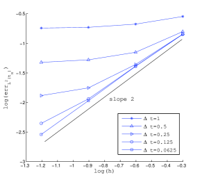
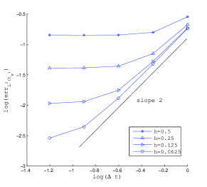
Fig. 1: Convergence w.r.t. $L^{2}(\Gamma(t_{N}))$ norm in Example 1.

Figure 2 shows the convergence behavior of the $L^{2}(H^{1})$-error with respect to space (in the left subfigure) and time (in the right subfigure). From the left subfigure it can be seen that the $L^{2}(H^{1})$-error is of order $O(h)$ in space. The results in the right subfigure indicate that on the meshes used in this experiment the $L^{2}(H^{1})$-error is dominated by the space error. Note that (very) large timesteps, even $\Delta t=1$, can be used (even for small $h$), which indicates that the method has good stability properties.

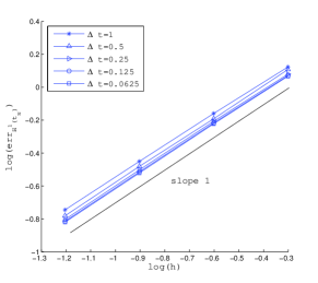
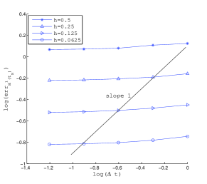
Fig. 2: Convergence w.r.t. $L^{2}(H^{1})$ norm in Example 1.

To illustrate the convergence behavior of $H^{1}$-errors with respect to time, we consider an experiment on the shrinking sphere, where the solution is given by $u(x,t)=e^{t},$ i.e. the function has maximal smoothness w.r.t. the spatial variable. A simple computation yields $f=\frac{\partial u}{\partial t}+\mathbf{w}\cdot\nabla_{\Gamma}u+({\,\operatorname{div_{\Gamma}}}\mathbf{w})u+\Delta_{\Gamma}u=\frac{\partial u}{\partial t}-u=0.$ The $L^{2}(H^{1})$-errors for this example are shown in Figure 3. From the left subfigure, we see that again the $L^{2}(H^{1})$-error is of order $O(h)$ in space, just as in the previous case. In the right subfigure we observe that the error converges in time with order $O(\Delta t)$.

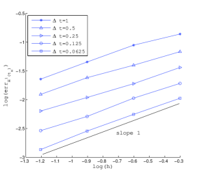
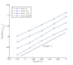
Fig. 3: Convergence w.r.t. $L^{2}(H^{1})$ norm for $u(x,t)=e^{t}$.

Example 2. In this example, we consider a surface diffusion problem as in (2) on a moving manifold. The initial manifold is given (as in [5]) by $\Gamma(0)=\{\,x\in\mathbb{R}^{3}~{}|~{}(x_{1}-x_{3}^{2})^{2}+x_{2}^{2}+x_{3}^{2}=1\,\}.$ The velocity field that transports the surface is

$$\mathbf{w}(x,t)=\big{(}0.1x_{1}\cos(t),0.2x_{2}\sin(t),0.2x_{3}\cos(t)\big{)}^{T}.$$

The initial concentration $u_{0}$ is chosen as $u_{0}(x)=1+x_{1}x_{2}x_{3}.$

We set $\Delta t=0.1$ and compute the problem until $T=8$. The mesh size of the spatial outer mesh is $h=0.125$. An approximate surface $\mathcal{S}^{h}$ is constructed in the same way as in Example 1. In Figure 4 we show the (aproximated) manifold and the discrete solution $u_{h}$ for different points in time.

\begin{overpic}[width=195.12767pt]{surf0000.eps} \end{overpic}

\begin{overpic}[width=195.12767pt]{surf0002.eps} \end{overpic}

\begin{overpic}[width=195.12767pt]{surf0010.eps} \end{overpic}

\begin{overpic}[width=195.12767pt]{surf0020.eps} \end{overpic}

\begin{overpic}[width=195.12767pt]{surf0030.eps} \end{overpic}

\begin{overpic}[width=195.12767pt]{surf0040.eps} \end{overpic}

Fig. 4: Example 2: solutions for $t=0,0.4,2,4,6,8$.

In this problem the total mass $M(t)=\int_{\Gamma(t)}u(\cdot,t)\,ds$ is conserved and equal to $M(0)=|\Gamma(0)|\approx 13.6083.$ We check how well the discrete analogon $M_{h}(t)=\int_{\Gamma_{h}(t)}u_{h}(\cdot,t)\,ds$ is conserved. In Figure 5, for $t\in[0,T]$ this quantity is illustrated for different mesh sizes $h$ and a fixed time step $\Delta t=0.1$. In Figure 5, the quantity is shown for different time steps $\Delta t$ and a fixed mesh size $h=0.125$. If we compute the average discrete mass $M_{h}:=\frac{1}{m}\sum_{j=1}^{m}M_{h}(t_{j})$, with $t_{1},\ldots,t_{m}$ the discrete time points (as shown in Fig. 5) we obtain for the absolute error $|M(0)-M_{h}|$ the numbers 0.2302, 0.0562, 0.0129, 0.0020 (corresponding to Fig. 5) and 0.4973, 0.1126, 0.0208, 0.0052 (corresponding to Fig. 5). These results indicate that the method has a satisfactory discrete mass conservation property with a rate of convergence that is second order both with respect to $h$ and $\Delta t$.

Finally we note that the errors in the discretization are caused not only by the space-time finite element discretization but also by the geometric errors caused by the approximation of $\mathcal{S}$ by $\mathcal{S}^{h}$.

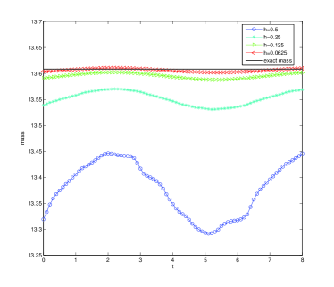
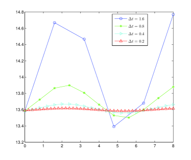
Fig. 5: Example 2: Discrete mass conservation.

8 Conclusions

In this paper we develop a mathematical framework for a new Eulerian finite element method for parabolic equations posed on evolving surfaces. The discretization method uses space-time elements. The space-time finite element method naturally relies on a space-time weak formulation. Such a formulation is introduced and shown to be well-posed. The analysis uses a smooth diffeomorphism between the space-time manifold and a reference domain. This theoretical framework does not allow to treat surfaces that undergo topological changes such as merging or splitting. The numerical method, however, can be applied in such situations. Stabiliy of the discrete method is derived only for a special case. Numerical experiments demonstrate stable behaviour and optimal convergence results in a more general setting. Extension of the finite element error analysis to more general problems is a topic of current research. In this paper, we consider only the case of piecewise linear (in space and time) finite elements. The method, however, is directly applicable with higher order finite elements. To benefit from the higher order approximation one needs a sufficiently accurate approximation of the continuous space-time manifold.

Acknowledgement

Funding by the National Science Foundation through the project DMS-1315993, the German Science Foundation (DFG) through the project RE 1461/4-1, and by the Russian Foundation for Basic Research through the projects 12-01-91330, 12-01-33084 is acknowledged. The authors thank Jörg Grande for his contribution to the implementation of the finite element method.

References

- [1] D. Adalsteinsson and J. A. Sethian, Transport and diffusion of material quantities on propagating interfaces via level set methods, J. Comput. Phys., 185 (2003), pp. 271–288.
- [2] B. Alberta, A. Johnson, J. Lewis, M. Raff, K. Roberts, and P. Walter, Molecular Biology of the Cell, Garland Science, New York, fouth ed., 2002.
- [3] A.Y. Chernyshenko and M.A. Olshanskii, Non-degenerate Eulerian finite element method for solving PDEs on surfaces, Rus. J. Num. Anal. Math. Model., 28 (2013), pp. 101–124.
- [4] A. Demlow and M.A. Olshanskii, An adaptive surface finite element method based on volume meshes, SIAM J. Numer. Anal., 50 (2012), pp. 1624–1647.
- [5] G. Dziuk, Finite elements for the Beltrami operator on arbitrary surfaces, in Partial differential equations and calculus of variations, S. Hildebrandt and R. Leis, eds., vol. 1357 of Lecture Notes in Mathematics, Springer, 1988, pp. 142–155.
- [6] G. Dziuk and C. Elliott, Finite elements on evolving surfaces, IMA J. Numer. Anal., 27 (2007), pp. 262–292.
- [7] , An Eulerian approach to transport and diffusion on evolving implicit surfaces, Comput Visual Sci, 13 (2010), pp. 17–28.
- [8] C. M. Elliott, B. Stinner, V Styles, and R. Welford, Numerical computation of advection and diffusion on evolving diffuse interfaces, IMA J. Numer. Anal., 31 (2011), pp. 786–812.
- [9] A. Ern and J.-L. Guermond, Theory and practice of finite elements, Springer, New York, 2004.
- [10] J. Grande, Finite element methods for parabolic equations on moving surfaces, Preprint 360, IGPM RWTH Aachen University, 2013. To appear in SIAM J. Sci. Comp.
- [11] J. Grande, M. A. Olshanskii, and A. Reusken, A space-time FEM for PDEs on evolving surfaces, in Proceedings of 11th World Congress on Computational Mechanics, E. Onate, J. Oliver, and A. Huerta, eds., Eccomas, 2014.
- [12] J. B. Greer, An improvement of a recent Eulerian method for solving PDEs on general geometries, J. Sci. Comput., 29 (2008), pp. 321–352.
- [13] S. Groß and A. Reusken, Numerical Methods for Two-phase Incompressible Flows, Springer, Berlin, 2011.
- [14] A.J. James and J. Lowengrub, A surfactant-conserving volume-of-fluid method for interfacial flows with insoluble surfactant, J. Comp. Phys., 201 (2004), pp. 685–722.
- [15] M. Olshanskii and A. Reusken, A finite element method for surface PDEs: matrix properties, Numer. Math., 114 (2009), pp. 491–520.
- [16] M.A. Olshanskii and A. Reusken, Error analysis of a space-time finite element method for solving PDEs on evolving surfaces, Preprint 376, IGPM RWTH Aachen University, 2013. submitted.
- [17] M. Olshanskii, A. Reusken, and J. Grande, A finite element method for elliptic equations on surfaces, SIAM J. Numer. Anal., 47 (2009), pp. 3339–3358.
- [18] M. Olshanskii, A. Reusken, and X. Xu, A stabilized finite element method for advection-diffusion equations on surfaces, IMA J. Numer. Anal., doi:10.1093/imanum/drt016 (2013).
- [19] J. A. Sethian, Theory, algorithms, and applications of level set methods for propagating interfaces, Acta Numerica, 5 (1996), pp. 309–395.
- [20] M. Vierling, Control-constrained parabolic optimal control problems on evolving surfaces - theory and variational discretization, Hamburger Beiträge zur Angewandten Mathematik 2011-10, University Hamburg, Department of Mathematics, 2011. arXiv:1106.0622v4.
- [21] Jian-Jun Xu and Hong-Kai Zhao, An Eulerian formulation for solving partial differential equations along a moving interface, Journal of Scientific Computing, 19 (2003), pp. 573–594.
- [22] E. Zeidler, Nonlinear Functional Analysis and its Applications, II/A, Springer, New York, 1990.