Surface waves in a stretched and sheared
incompressible elastic material

Abstract

In this paper we analyze the effect of a combined pure homogeneous strain and simple shear in a principal plane of the latter on the propagation of surface waves for an incompressible isotropic elastic half-space whose boundary is normal to the glide planes of the shear. This generalizes previous work in which, separately, pure homogeneous strain and simple shear were considered. For a special class of materials the secular equation is obtained in explicit form and then specialized to recover results obtained previously for the two cases mentioned above. A method for obtaining the secular equation for a general form of strain-energy function is then outlined. In general this is very lengthy and the result is not listed, but, for the case in which there is no normal stress on the half-space boundary, the result is given, for illustration, in respect of the so-called generalized Varga material. Numerical results are given to show how the surface wave speed depends on both the underlying pure homogeneous strain and the superimposed simple shear. Further numerical results are provided for the Gent model of limiting chain extensibility.

1 Introduction

The vibration and wave propagation characteristics of rubberlike solids are important for practical applications in, for example, engine mountings and seismic isolators, and an understanding of these characteristics is therefore of crucial importance. There have been many contributions in recent years to the analysis of, in particular, vibrations and surface and interfacial waves in finitely deformed elastic bodies, but relatively little attention has been given to shearing deformations, for which the orientation of the principal axes of deformation depends on the magnitude of the shear. In this paper we are concerned with the influence of a simple shear combined with a pure homogeneous strain on the propagation of surface waves.

Analysis of surface waves in a half-space subject to pure homogeneous deformation dates back to the classic paper of Hayes and Rivlin [1], which was concerned primarily with compressible materials, while Flavin [2] considered the same problem for an incompressible material, specifically the Mooney-Rivlin material (for completeness, mention should be made of early and noteworthy articles by Biot [3] and by Buckens [4] and the related work of Biot summarized in [5]). A more detailed analysis was provided for general incompressible elastic materials by Dowaikh and Ogden [6], who also examined the connection between surface wave propagation and stability of the half-space, again for the case of pure homogeneous strain. We refer to this latter paper, that by Chadwick [7] and the recent contribution by Fu [8], for pointers to the relevant literature. The only paper thus far that deals with the influence of shear on surface wave propagation appears to be that by Connor and Ogden [9], and the closely related paper [10]. These are concerned with simple shear and give explicit results for a certain class of incompressible materials, of which the best known representative is the Mooney-Rivlin model for rubberlike solids.

The purpose of this paper is to extend the analysis in the above papers to the situation in which a simple shear is combined with a pure homogeneous deformation and for a general incompressible isotropic hyperelastic material. These extensions are motivated by several factors. First, one can easily picture situations of practical interest where a solid is stretched and sheared: for instance, a rubber isolator under a bridge is subjected to a vertical compression and is then sheared as a result of thermal extensions and contractions of the roadway. Also, the combination of stretch and shear theoretically allows a square block of incompressible material to be maintained in a deformed state with no shear tractions nor normal tractions on its faces [11], in contrast to simple shear and its associated Poynting effect. Finally, the quite recent application of nonlinear elasticity to the modelling of some biological tissues (see Humphrey [12] or Holzapfel and Ogden [13]) has highlighted the need for solutions valid for more general strain-energy functions because the functions used for biomaterials are usually more complicated than those used for rubberlike materials.

In Section 2 the basic equations for the (static) finite deformation consisting of a pure homogeneous strain (or triaxial stretch) followed by a simple shear in a principal plane of the pure homogeneous strain are summarized for an incompressible isotropic elastic material. The corresponding equations for infinitesimal surface waves superimposed on this finite deformation are then outlined. The equations and zero incremental traction boundary conditions are applied to surface waves propagating in the direction of shear and parallel to a half-space whose normal lies within the plane of shear. The secular equation for the wave speed is then obtained in implicit form in respect of a general strain-energy function.

This equation in examined in detail in Section 3. For a class of materials that includes the Mooney-Rivlin strain energy, the secular equation is given in simple explicit form, which relates the wave speed to the material parameters, the deformation and the normal stress on the half-space associated with the underlying finite deformation. Next, an alternative approach is outlined, which enables the secular equation to be made explicit in the more general case. However, since this is very complicated we illustrate the results by considering a generalized form of the Varga material model. Specifically, in the absence of normal loads on the half-space boundary we obtain the secular equation in relatively simple explicit form as a quartic for the squared wave speed. On the other hand, in the presence of normal loads we give the corresponding explicit form of bifurcation condition (corresponding to zero wave speed), which consists of two separate equations. For each of the material models considered numerical results are described in Section 4, illustrating the dependence of the wave speed separately on the stretching and shearing parts of the underlying deformation. Finally, for comparison, some limited results are given for a model of finite chain extensibility of rubberlike solids originally due to Gent [14], and recently used by Horgan and Saccomandi [15] to model strain-hardening arterial walls.

In closing this Introduction, we note that the method and the results presented in the paper are easily extended to a generic type of homogeneous pre-strain having a plane of symmetry, and to unconstrained (compressible) solids. The assumptions of combined stretch and shear and of incompressibility lead to some simplifications and to neat algebraic expressions, but they are inessential and should not be viewed as restrictive.

2 Basic equations

2.1 Finite static deformations

Let $(X_{1},X_{2},X_{3})$ be a rectangular Cartesian coordinate system. Consider a homogeneous semi-infinite body occupying the region $X_{2}\geq 0$ in its natural (unstressed) configuration. Suppose that the body is composed of an incompressible isotropic elastic material characterized by a constant mass density $\rho$ and a strain-energy function $W(\lambda_{1},\lambda_{2},\lambda_{3})$ (per unit volume) written as a (symmetric) function of the (positive) principal stretches $(\lambda_{1},\lambda_{2},\lambda_{3})$, which satisfy the incompressibility constraint

$$\lambda_{1}\lambda_{2}\lambda_{3}=1.$$ (2.1)

The body is subjected first to a finite pure homogeneous triaxial stretch with principal stretch ratios $\mu_{1},\mu_{2},\mu_{3}$ ($\mu_{1}\mu_{2}\mu_{3}=1$) and then to a finite simple shear of amount $\kappa$, so that a particle initially at ($X_{1},X_{2},X_{3}$) is displaced to ($\hat{x}_{1},\hat{x}_{2},\hat{x}_{3}$) according to

$$\hat{x}_{1}=\mu_{1}X_{1}+\kappa\mu_{2}X_{2},\quad\hat{x}_{2}=\mu_{2}X_{2},\quad\hat{x}_{3}=\mu_{3}X_{3}.$$ (2.2)

     

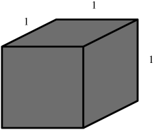
(a) Unit cube

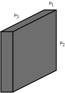
(b) Triaxial stretch

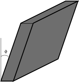
(c) Simple shear

Figure 1: Triaxial stretch followed by simple shear of a unit cube.

Figure 1 shows the successive deformations of a unit cube in the half-space; in Figure 1(c) the angle $\phi$ is the angle of shear, which is given by $\tan\phi=\kappa$.

The deformation gradient $\mathbf{F}$ associated with the deformation (2.2) has components

$$\begin{bmatrix}\mu_{1}&\kappa\mu_{2}&0\\ 0&\mu_{2}&0\\ 0&0&\mu_{3}\end{bmatrix}.$$ (2.3)

Let $x_{1},x_{2},x_{3}$, be the rectangular Cartesian coordinates associated with the (orthogonal) principal axes of $\mathbf{FF}^{T}$ (the left Cauchy-Green deformation tensor), one of which is the $\hat{x}_{3}$ direction, so that $x_{3}=\hat{x}_{3}$. Within the $(x_{1},x_{2})$ plane let the $x_{1}$ principal axis make an angle $\theta$ with the $\hat{x}_{1}$ axis measured in the anticlockwise sense. Then the coordinates ($\hat{x}_{1},\hat{x}_{2},\hat{x}_{3}$) are related to ($x_{1},x_{2},x_{3}$) through a rotation according to

$$\hat{x}_{i}=\Omega_{ij}x_{j},\quad[\Omega_{ij}]=\begin{bmatrix}\cos\theta&-\sin\theta&0\\ \sin\theta&\cos\theta&0\\ 0&0&1\end{bmatrix}.$$ (2.4)

The principal stretches, subject to (2.1), and the angle $\theta$ are given in terms of the components (2.3) by

$$\lambda_{1}^{2}\cos^{2}\theta+\lambda_{2}^{2}\sin^{2}\theta=\mu_{1}^{2}+\mu_{2}^{2}\kappa^{2},$$

$$(\lambda_{1}^{2}-\lambda_{2}^{2})\cos\theta\sin\theta=\mu_{2}^{2}\kappa,$$

$$\lambda_{1}^{2}\sin^{2}\theta+\lambda_{2}^{2}\cos^{2}\theta=\mu_{2}^{2},$$ (2.5)

from which we obtain

$$\lambda_{1}\pm\lambda_{2}=\sqrt{(\mu_{1}\pm\mu_{2})^{2}+\kappa^{2}\mu_{2}^{2}},\quad\lambda_{3}=1/(\mu_{1}\mu_{2}),$$ (2.6)

and

$$\tan 2\theta=2\mu_{2}^{2}\kappa/(\mu_{1}^{2}-\mu_{2}^{2}+\kappa^{2}\mu_{2}^{2})$$ (2.7)

(see, for example, [16, 11, 17]). When the material is sheared but not stretched ($\mu_{1}=\mu_{2}=\mu_{3}=1$), for example, the well-known formulas

$$\lambda_{1,2}=(\sqrt{4+\kappa^{2}}\pm\kappa)/2,\quad\lambda_{3}=1,\quad\tan 2\theta=2/\kappa,$$ (2.8)

are recovered.

Let $\sigma_{1},\sigma_{2},\sigma_{3}$ denote the principal Cauchy stresses. Since the material is isotropic the principal axes of Cauchy stress coincide with those of $\mathbf{FF}^{T}$, and hence, analogously to (2.1), we may express the components of the Cauchy stress on the axes associated with the coordinates ($\hat{x}_{1},\hat{x}_{2},\hat{x}_{3}$), denoted by $\hat{\sigma}_{ij}$, as

$$\hat{\sigma}_{11}=\sigma_{1}\cos^{2}\theta+\sigma_{2}\sin^{2}\theta,$$

$$\hat{\sigma}_{12}=(\sigma_{1}-\sigma_{2})\sin\theta\cos\theta,$$

$$\hat{\sigma}_{22}=\sigma_{1}\sin^{2}\theta+\sigma_{2}\cos^{2}\theta,$$ (2.9)

with $\hat{\sigma}_{13}=\hat{\sigma}_{23}=0,\,\hat{\sigma}_{33}=\sigma_{3}$.

In terms of the strain-energy function, the principal Cauchy stresses are given by

$$\sigma_{i}=\lambda_{i}\frac{\partial W}{\partial\lambda_{i}}-p,\quad i\in\{1,2,3\}\quad\mbox{no sum over $i$},$$ (2.10)

where $p$ is a Lagrange multiplier associated with the constrain (2.1).

The initial half-space $X_{2}\geq 0$ becomes the half-space $\hat{x}_{2}\geq 0$ after the deformation described above, and the load on its boundary $\hat{x}_{2}=0$ has normal component $\hat{\sigma}_{22}$ and shear component $\hat{\sigma}_{12}$. We now consider the propagation of surface waves in this half-space.

2.2 Superimposed infinitesimal surface waves

Now consider a surface (Rayleigh) wave propagating with speed $v$ and wave number $k$ in the $\hat{x}_{1}$ direction in the considered deformed half-space ($\hat{x}_{2}\geq 0$), with attenuation in the $\hat{x}_{2}$ direction. We emphasize, as noted above and in contrast to many previous studies of surface waves in deformed materials, these directions do not coincide with the principal directions $(x_{1},x_{2})$ of strain for the underlying pre-deformation. It seems that the only paper considering the propagation of non-principal surface waves over a non-principal plane is that by Connor and Ogden [9], where the problem was solved for a sheared half-space ($\mu_{1}=\mu_{2}=\mu_{3}=1$) and for a specific class of materials (see also the related paper by Connor and Ogden [10]).

Let the incremental displacement $\mathbf{u}$ associated with the wave have components $\hat{u}_{i},\,i\in\{1,2,3\}$ in the coordinates system ($\hat{x}_{1},\hat{x}_{2},\hat{x}_{3}$), with dependence, in general, on $(\hat{x}_{1},\hat{x}_{2},\hat{x}_{3},t)$, where $t$ is time. The corresponding components $\hat{s}_{ij}$ of the incremental nominal stress tensor are then given by

$$\hat{s}_{ij}=\hat{B}_{ijkl}\frac{\partial\hat{u}_{l}}{\partial\hat{x}_{k}}+p\frac{\partial\hat{u}_{i}}{\partial\hat{x}_{j}}-\hat{p}\delta_{ij},$$ (2.11)

where $\hat{B}_{ijkl}$ are the components of $\mathbf{B}$, the tensor of first-order elastic moduli associated with the underlying deformation, and $\hat{p}$ is the incremental counterpart of $p$. The non-vanishing components of the elasticity tensor $\mathbf{B}$, denoted $B_{ijkl}$, in the coordinate system ($x_{1},x_{2},x_{3}$) are given by

$$B_{iijj}=\lambda_{i}\lambda_{j}W_{ij},$$

$$B_{ijij}=(\lambda_{i}W_{i}-\lambda_{j}W_{j})\lambda_{i}^{2}/(\lambda_{i}^{2}-\lambda_{j}^{2})\quad i\neq j,$$

$$B_{ijji}=B_{jiij}=B_{ijij}-\lambda_{i}W_{i}\quad i\neq j$$ (2.12)

(see, for example, [18, 6, 19]), where $W_{i}:=\partial W/\partial\lambda_{i},\,W_{ij}:=\partial^{2}W/\partial\lambda_{i}\partial\lambda_{j}$. Note that expressions for $B_{ijij}$ in the case $\lambda_{i}=\lambda_{j},\,i\neq j$, may be obtained by a limiting process.

The two sets of components of $\mathbf{B}$ are related by

$$\hat{B}_{ijkl}=\Omega_{ip}\Omega_{jq}\Omega_{kr}\Omega_{ls}B_{pqrs}$$ (2.13)

and they satisfy the symmetry properties

$$B_{ijkl}=B_{klij},\quad\hat{B}_{ijkl}=\hat{B}_{klij}.$$ (2.14)

Also, note that for $i,j\in\{1,2\}$, in particular, $\mathbf{B}$ has six non-zero entries in the $(x_{1},x_{2},x_{3})$ system, namely $B_{1111}$, $B_{2222}$, $B_{1122}$, $B_{1221}$, $B_{1212}$, and $B_{2121}$, whereas in the $(\hat{x}_{1},\hat{x}_{2},\hat{x}_{3})$ system it has ten: $\hat{B}_{1111}$, $\hat{B}_{2222}$, $\hat{B}_{1122}$, $\hat{B}_{1221}$, $\hat{B}_{1212}$, $\hat{B}_{2121}$, the counterparts of those above, together with $\hat{B}_{1112}$, $\hat{B}_{1121}$, $\hat{B}_{1222}$, and $\hat{B}_{2122}$.

For surface waves propagating on a half-space subject to a pure homogeneous stretch and no shear ($\kappa=0$), Dowaikh and Ogden [6] found it convenient to introduce the shorthand notations

$$\alpha=B_{1212},\quad\gamma=B_{2121}=\lambda_{1}^{-2}\lambda_{2}^{2}\alpha,\quad 2\beta=B_{1111}+B_{2222}-2B_{1122}-2B_{1221}.$$ (2.15)

The corresponding quantities in the $(\hat{x}_{1},\hat{x}_{2},\hat{x}_{3})$ system are obtained by using (2.13) in the form

$$\hat{\alpha} :=\hat{B}_{1212}=\alpha\cos^{4}\theta+2\beta\sin^{2}\theta\cos^{2}\theta+\gamma\sin^{4}\theta,$$

$$\hat{\gamma} :=\hat{B}_{2121}=\alpha\sin^{4}\theta+2\beta\sin^{2}\theta\cos^{2}\theta+\gamma\cos^{4}\theta,$$

$$2\hat{\beta} :=\hat{B}_{1111}+\hat{B}_{2222}-2\hat{B}_{1122}-2\hat{B}_{1221}=2\beta-6(2\beta-\alpha-\gamma)\sin^{2}\theta\cos^{2}\theta.$$ (2.16)

It is easily checked that neither $\alpha$, $\gamma$, $\beta$ nor $\hat{\alpha}$, $\hat{\gamma}$, $\hat{\beta}$ depend separately on the constant Cauchy stress components ($\sigma_{1},\sigma_{2},\sigma_{3}$) (or equivalently on $\hat{\sigma}_{ij}$). It follows from (2.2) that

$$\hat{\alpha}-\hat{\gamma}=(\alpha-\gamma)\cos 2\theta,\quad\hat{\alpha}+\hat{\gamma}-2\hat{\beta}=(\alpha+\gamma-2\beta)\cos 4\theta.$$ (2.17)

From the latter it follows that if the equality $\alpha+\gamma-2\beta=0$ is satisfied, as it is for certain forms of the strain-energy function, then we also have $\hat{\alpha}+\hat{\gamma}-2\hat{\beta}=0$ for any angle $\theta$. In such a case the equality is said to be ‘structurally invariant’ [20].

Finally in this section, we note that the strong ellipticity condition may be expressed in the form

$$\alpha>0,\quad\beta+\sqrt{\alpha\gamma}>0$$ (2.18)

(see, for example, Dowaikh and Ogden [6] and Chadwick [7]). It follows immediately that $\hat{\alpha}>0$, but the counterpart of the second inequality in (2.18) for the $(\hat{x}_{1},\hat{x}_{2},\hat{x}_{3})$ system is not so simple, and is not therefore given here.

2.3 Equations of motion and boundary conditions

We now restrict attention to waves of the form

$$\mathbf{u}(\hat{x}_{1},\hat{x}_{2},t)=\mathbf{U}(k\hat{x}_{2})e^{{\rm i}k(\hat{x}_{1}-vt)},$$ (2.19)

independent of $\hat{x}_{3}$, where $\mathbf{U}$ is a function of $k\hat{x}_{2}$, $k$ is the wave number and $v$ the wave speed. This must satisfy the incremental equations of motion and the incremental incompressibility constraint. Respectively, these are

$$\frac{\partial\hat{s}_{ji}}{\partial\hat{x}_{j}}=\rho\frac{\partial^{2}\hat{u}_{i}}{\partial t^{2}},\quad\hat{u}_{i,i}=0\quad\text{in}\ \hat{x}_{2}>0.$$ (2.20)

Additionally, we impose the condition of zero incremental traction on the plane boundary, so that

$$\hat{s}_{2i}=0\quad\text{on}\ \hat{x}_{2}=0,\quad i=1,2,3.$$ (2.21)

In view of equations (2.19) and (2.11), $\hat{s}_{ij}$ and $\hat{p}$ take forms similar to that of the displacement $\mathbf{u}$, that is

$$\{\hat{s}_{ij}(\hat{x}_{1},\hat{x}_{2},t),\hat{p}(\hat{x}_{1},\hat{x}_{2},t)\}=\{kS_{ij}(k\hat{x}_{2}),{\rm i}kP(k\hat{x}_{2})\}e^{{\rm i}k(\hat{x}_{1}-vt)},$$ (2.22)

where we have introduced the functions $S_{ij}$ and $P$ of $k\hat{x}_{2}$ It is a straightforward exercise to check that the in-plane equations decouple from the out-of-plane equations, so that there is no loss of generality in taking $U_{3}=0$. The incremental equations of motion and incompressibility (2.20) and (2.21) then specialize to

$${\rm i}S_{11}+S^{\prime}_{21}=-XU_{1},\quad{\rm i}S_{12}+S^{\prime}_{22}=-XU_{2},\quad{\rm i}U_{1}+U^{\prime}_{2}=0,$$ (2.23)

where $X:=\rho v^{2}$ and a prime signifies differentiation with respect to the argument $k\hat{x}_{2}$.

It is convenient to introduce the quantities

$$\tau_{1}=-{\rm i}S_{21},\quad\tau_{2}=-{\rm i}S_{22},$$ (2.24)

which are functions of $\hat{x}_{2}$ proportional to the incremental tractions on the planes parallel to the boundary. Thus, from the incremental boundary conditions (2.21), we have

$$\tau_{1}(0)=\tau_{2}(0)=0.$$ (2.25)

The expressions

$$S_{11}={\rm i}(\hat{B}_{1111}+p)U_{1}+{\rm i}\hat{B}_{1112}U_{2}+\hat{B}_{1121}U_{1}^{\prime}+\hat{B}_{1122}U_{2}^{\prime}-{\rm i}P,$$

$${\rm i}\tau_{2}={\rm i}\hat{B}_{1122}U_{1}+{\rm i}\hat{B}_{1222}U_{2}+\hat{B}_{2122}U_{1}^{\prime}+(\hat{B}_{2222}+p)U_{2}^{\prime}-{\rm i}P,$$

$${\rm i}\tau_{1}={\rm i}\hat{B}_{1121}U_{1}+{\rm i}(\hat{B}_{1221}+p)U_{2}+\hat{\gamma}U_{1}^{\prime}+\hat{B}_{2122}U_{2}^{\prime},$$

$$S_{12}={\rm i}\hat{B}_{1112}U_{1}+{\rm i}\hat{\alpha}U_{2}+(\hat{B}_{1221}+p)U_{1}^{\prime}+\hat{B}_{1222}U_{2}^{\prime}$$ (2.26)

may be derived from equations (2.19), (2.22) and (2.11).

The short-hand notations defined by

$$\hat{\nu}_{12}=\hat{B}_{1222}-\hat{B}_{1112}=\textstyle{\frac{1}{2}}[\gamma-\alpha+(2\beta-\alpha-\gamma)\cos 2\theta]\sin 2\theta,$$

$$\hat{\nu}_{21}=\hat{B}_{1121}-\hat{B}_{2122}=\textstyle{\frac{1}{2}}[\gamma-\alpha-(2\beta-\alpha-\gamma)\cos 2\theta]\sin 2\theta,$$ (2.27)

prove useful in rewriting the equations of motion in a convenient form. Indeed, a few manipulations and use of (2.23), (2.3) and (2.3) lead to the first-order differential system

$${\bf\mbox{\boldmath$\xi$}^{\prime}}={\rm i}\mathbf{N}\mbox{\boldmath$\xi$},\quad\mbox{\boldmath$\xi$}:=[U_{1},U_{2},\tau_{1},\tau_{2}]^{T},$$ (2.28)

where

$$\mathbf{N}=\begin{bmatrix}\mathbf{N}_{1}&\mathbf{N}_{2}\\ \mathbf{K}^{(1)}&\mathbf{N}_{1}^{T}\end{bmatrix},\quad\mathbf{N}_{1}=\begin{bmatrix}-\hat{\nu}_{21}/\hat{\gamma}&-(\hat{\gamma}-\hat{\sigma}_{22})/\hat{\gamma}\\ -1&0\end{bmatrix},\quad\mathbf{N}_{2}=\begin{bmatrix}1/\hat{\gamma}&0\\ 0&0\end{bmatrix},$$

$$\mathbf{K}^{(1)}=\begin{bmatrix}X-2(\hat{\beta}+\hat{\gamma}-\hat{\sigma}_{22})+\hat{\nu}^{2}_{21}/\hat{\gamma}&\hat{\nu}_{12}+\hat{\nu}_{21}(\hat{\gamma}-\hat{\sigma}_{22})/\hat{\gamma}\\ \hat{\nu}_{12}+\hat{\nu}_{21}(\hat{\gamma}-\hat{\sigma}_{22})/\hat{\gamma}&X-\hat{\alpha}+(\hat{\gamma}-\hat{\sigma}_{22})^{2}/\hat{\gamma}\end{bmatrix}.$$ (2.29)

The classical approach to solving the equations of motion (2.28) subject to (2.25) consists of writing the solution as a decaying exponential function, such as

$$\mbox{\boldmath$\xi$}(kx_{2})=\mbox{\boldmath$\xi$}^{0}e^{{\rm i}qkx_{2}},\quad\Im(q)>0,$$ (2.30)

and then solving the eigenvalue problem $\mathbf{N}\mbox{\boldmath$\xi$}^{0}=q\mbox{\boldmath$\xi$}^{0}$. Its solution is of the form

$$\mbox{\boldmath$\xi$}(kx_{2})=A_{1}\mbox{\boldmath$\xi$}^{1}e^{{\rm i}q_{1}kx_{2}}+A_{2}\mbox{\boldmath$\xi$}^{2}e^{{\rm i}q_{2}kx_{2}},$$ (2.31)

where $A_{1}$, $A_{2}$ are constants such that (2.25) is satisfied. Explicitly, $q_{1}$ and $q_{2}$ are the complex roots of the propagation condition $\det(\mathbf{N}-q\mathbf{I})=0$ with positive imaginary parts, where I is the fourth-order identity. The resulting equation is the quartic

$$\hat{\gamma}q^{4}+2\hat{\nu}_{21}q^{3}+(2\hat{\beta}-X)q^{2}+2\hat{\nu}_{12}q+\hat{\alpha}-X=0$$ (2.32)

for $q$, while $\mbox{\boldmath$\xi$}^{i}$, $i=1,2$ may be taken as proportional to any column vector of the matrix adjoint to $\mathbf{N}-q_{i}\mathbf{I}$. If we take the third such column, for example, then

$$\mbox{\boldmath$\xi$}^{i}=[q_{i}^{2},-q_{i},q_{i}(\hat{\gamma}q_{i}^{2}+\hat{\nu}_{21}q_{i}-\hat{\gamma}+\hat{\sigma}_{22}),-(\hat{\gamma}-\hat{\sigma}_{22})q_{i}^{2}+\hat{\nu}_{12}q_{i}+\hat{\alpha}-X]^{T}.$$ (2.33)

The boundary conditions $\mbox{\boldmath$\xi$}(0)=[U_{1}(0),U_{2}(0),0,0]^{T}$ then yield a homogeneous system of two linear equations for the two unknowns $A_{1}$, $A_{2}$, whose determinant must be zero. This leads to the secular equation for the surface wave speed, written in the implicit form

$$\hat{\gamma}(\hat{\alpha}-X)(q_{1}^{2}+q_{1}q_{2}+q_{2}^{2})-(\hat{\gamma}-\hat{\sigma}_{22})(\hat{\gamma}q_{1}^{2}q_{2}^{2}+\hat{\alpha}-X)\\ +[\hat{\nu}_{12}\hat{\nu}_{21}-(\hat{\gamma}-\hat{\sigma}_{22})^{2}]q_{1}q_{2}+[\hat{\nu}_{12}\hat{\gamma}q_{1}q_{2}+\hat{\nu}_{21}(\hat{\alpha}-X)](q_{1}+q_{2})=0.$$ (2.34)

It remains implicit as long as $q_{1}$ and $q_{2}$ are not expressed explicitly.

3 Explicit secular equations

Here the problem of an incremental surface wave propagating over the surface of a stretched and sheared incompressible half-space is solved, up to the explicit derivation of the secular equation giving the speed of the Rayleigh wave.

3.1 Secular equation for materials with $2\beta=\alpha+\gamma$

Consider the Mooney-Rivlin strain-energy function

$$W=\textstyle{\frac{1}{2}}C(\lambda_{1}^{2}+\lambda_{2}^{2}+\lambda_{3}^{2}-3)+\textstyle{\frac{1}{2}}D(\lambda_{1}^{2}\lambda_{2}^{2}+\lambda_{2}^{2}\lambda_{3}^{2}+\lambda_{3}^{2}\lambda_{1}^{2}-3),$$ (3.1)

where $C$ and $D$ are constant material parameters. For (3.1), $\alpha$, $\gamma$ and $\beta$ reduce to

$$\alpha=\lambda_{1}^{2}(C+D\lambda_{3}^{2}),\quad\gamma=\lambda_{2}^{2}(C+D\lambda_{3}^{2}),\quad 2\beta=(\lambda_{1}^{2}+\lambda_{2}^{2})(C+D\lambda_{3}^{2}),$$ (3.2)

and so it is apparent that Mooney-Rivlin materials belong to the general class of materials with energy function such that

$$2\beta=\alpha+\gamma.$$ (3.3)

This class has the remarkable property that the propagation condition for inhomogeneous plane waves with displacement proportional to $\Re\{\exp[{\rm i}k(\hat{x}_{1}+q\hat{x}_{2}-vt)]\}$ always admits $q^{2}+1$ as a factor when the body is maintained in an arbitrary state of static homogeneous deformation. In fact, Pichugin [21] proved that this class is the most general one admitting this factorization.

Returning to the propagation condition (2.32) and using (2.1), we find that when (3.3) holds the quantities appearing in the quartic (2.32) simplify to

$$\hat{\alpha}=\gamma\lambda_{2}^{-2}\left(\mu_{1}^{2}+\mu_{2}^{2}\kappa^{2}\right),\quad\hat{\gamma}=\gamma\lambda_{2}^{-2}\mu_{2}^{2},\quad\hat{\nu}_{21}=\hat{\nu}_{12}=-\gamma\lambda_{2}^{-2}\mu_{2}^{2}\kappa,$$

$$2\hat{\beta}=\gamma\lambda_{2}^{-2}\left[\mu_{1}^{2}+\mu_{2}^{2}\left(1+\kappa^{2}\right)\right],\quad X=\gamma\lambda_{2}^{-2}\mu_{2}^{2}\left(\mu_{1}^{2}/\mu_{2}^{2}-\eta^{2}\right),$$ (3.4)

where the quantity

$$\eta:=\dfrac{\mu_{1}}{\mu_{2}}\sqrt{1-\dfrac{\lambda_{2}^{2}}{\mu_{1}^{2}}\dfrac{X}{\gamma}}$$ (3.5)

has been introduced in the last equality. Then, after removal of the factor $\hat{\gamma}\neq 0$, the quartic (2.32) factorizes as expected to give

$$(q^{2}+1)(q^{2}-2\kappa q+\kappa^{2}+\eta^{2})=0,$$ (3.6)

and its roots with positive imaginary parts are

$$q_{1}={\rm i},\quad q_{2}=\kappa+{\rm i}\eta.$$ (3.7)

In passing, we note that the condition $\Im(q_{i})>0$ for decay of the wave yields an upper bound on the admissible wave speed, such that

$$0\leq X=\rho v^{2}\leq\mu_{1}^{2}\lambda_{2}^{-2}\gamma,$$ (3.8)

with the limiting value $\mu_{1}^{2}\lambda_{2}^{-2}\gamma$ corresponding to a body wave not a surface wave (which requires strict inequality).

Finally, substituting the values (3.7) for $q_{1}$ and $q_{2}$ into (2.34), we arrive at the explicit secular equation

$$\eta^{3}+\eta^{2}+(3+\kappa^{2}-2\bar{\sigma}_{22})\eta-(1-\bar{\sigma}_{22})^{2}=0,$$ (3.9)

where $\bar{\sigma}_{22}:=\lambda_{2}^{2}\hat{\sigma}_{22}/(\mu_{2}^{2}\gamma)$. This secular equation is identical (apart from notational differences) to that obtained when the material is stretched but not sheared ($\kappa=0$) [2, 6] or when the material is sheared but not stretched ($\mu_{i}=1$) [9].

In the case of the Mooney-Rivlin strain energy (3.1), $\gamma\lambda_{2}^{-2}=C+D/(\mu_{1}\mu_{2})^{2}$, so that both $\eta$ and $\bar{\sigma}_{22}$ are independent of the amount of shear $\kappa$. Of course $\eta_{R}$, the positive real root of the cubic (3.9), depends on $\kappa$. By differentiation we find that $\partial\eta_{R}/\partial(\kappa^{2})=-\eta_{R}^{2}/[2\eta_{R}^{3}+\eta_{R}^{2}+(1-\bar{\sigma}_{22})^{2}]<0$ and so that, by (3.1)₄, the surface wave speed is a monotone increasing function of the amount of shear. Hence for Mooney-Rivlin materials subject to a given triaxial stretch $\mu_{1},\mu_{2},\mu_{3}$, the greater the subsequent shear is, the faster the Rayleigh wave propagates.

In the limit $X=0$ the secular equation (3.9) reduces to the bifurcation equation. This defines a curve in ($\mu_{i},\kappa,\bar{\sigma}_{22}$)-space that separates the region where the surface wave exists (and is unique) and the half-space is stable from the region where the surface wave does not exist and the half-space might become unstable (see Chadwick and Jarvis [22] or Dowaikh and Ogden [6]). The bifurcation equation is

$$\left(\dfrac{\mu_{1}}{\mu_{2}}\right)^{3}+\left(\dfrac{\mu_{1}}{\mu_{2}}\right)^{2}+(3+\kappa^{2}-2\bar{\sigma}_{22})\left(\dfrac{\mu_{1}}{\mu_{2}}\right)-(1-\bar{\sigma}_{22})^{2}=0.$$ (3.10)

When there is no normal Cauchy pre-stress in the $\hat{x}_{2}$ direction ($\bar{\sigma}_{22}=0$), the bifurcation criterion becomes universal with respect to the entire class of incompressible materials satisfying (3.3) since it does not depend on the material parameters associated with a specific strain energy, but only on the pre-stretch and the amount of shear.

3.2 Secular equation for a general strain energy

For a general (incompressible, isotropic) strain-energy function ($2\beta\neq\alpha+\gamma$), the propagation condition (2.32) does not factorize as in (3.6) and it is difficult in general to use the quartic (2.32) for the derivation of an explicit secular equation. Instead, we employ the method of the ‘polarization vector’ devised by Currie [23] and based on the fundamental equations

$$\overline{\mathbf{U}}(0)\cdot[\mathbf{K}^{(n)}\mathbf{U}(0)]=0.$$ (3.11)

Here, the symmetric $2\times 2$ matrix $\mathbf{K}^{(n)}$ is the lower left block of $\mathbf{N}^{n}$, where $n$ is any positive or negative integer. Thus, for instance, $\mathbf{K}^{(1)}$ is given by (2.3)₄, and we find that $\mathbf{K}^{(-1)}$ and $\mathbf{K}^{(2)}$ are given by

$$\frac{1}{X-\hat{\alpha}}\begin{bmatrix}\hat{\gamma}(X-\hat{\alpha})+(\hat{\gamma}-\hat{\sigma}_{22})^{2}&-\hat{\nu}_{21}(X-\hat{\alpha})+\hat{\nu}_{12}(\hat{\gamma}-\hat{\sigma}_{22})\\ -\hat{\nu}_{21}(X-\hat{\alpha})+\hat{\nu}_{12}(\hat{\gamma}-\hat{\sigma}_{22})&\hat{\nu}_{12}^{2}-(X-\hat{\alpha})(X-2\hat{\beta}-2\hat{\gamma}+2\hat{\sigma}_{22})\end{bmatrix},$$ (3.12)

and

$$-\begin{bmatrix}2\hat{\nu}_{21}K^{(1)}_{11}/\hat{\gamma}+2K^{(1)}_{12}&\hat{\nu}_{21}K^{(1)}_{12}/\hat{\gamma}+K^{(1)}_{22}+(\hat{\gamma}-\hat{\sigma}_{22})K^{(1)}_{11}/\hat{\gamma}\\ \hat{\nu}_{21}K^{(1)}_{12}/\hat{\gamma}+K^{(1)}_{22}+(\hat{\gamma}-\hat{\sigma}_{22})K^{(1)}_{11}/\hat{\gamma}&2(\hat{\gamma}-\hat{\sigma}_{22})K^{(1)}_{12}/\hat{\gamma}\end{bmatrix},$$ (3.13)

respectively. Here $K^{(2)}_{11}$ and $K^{(2)}_{12}$ are linear in $X$ and $K^{(2)}_{22}$ is independent of $X$.

Now, the fundamental equations (3.11), written in turn for $n=1,-1,2$, yield the homogeneous system

$$\begin{bmatrix}K^{(1)}_{11}&K^{(1)}_{12}&K^{(1)}_{22}\\ K^{(-1)}_{11}&K^{(-1)}_{12}&K^{(-1)}_{22}\\ K^{(2)}_{11}&K^{(2)}_{12}&K^{(2)}_{22}\end{bmatrix}\begin{bmatrix}U_{1}(0)\overline{U}_{1}(0)\\ U_{1}(0)\overline{U}_{2}(0)+\text{c.c.}\\ U_{2}(0)\overline{U}_{2}(0)\end{bmatrix}=\begin{bmatrix}0\\ 0\\ 0\end{bmatrix},$$ (3.14)

where c.c. denotes the complex conjugate of the preceding term. The determinant of the left-hand matrix in (3.14) must be zero, and the resulting equation is the explicit secular equation for surface waves in a stretched and sheared incompressible material. It is a quartic in $X$, but since its explicit expression is very lengthy we do not give it here, although it has been obtained using Maple and Mathematica. We note, however, that in the stress-free configuration ($\hat{\sigma}_{22}=0,\mu_{i}=1,\kappa=0$) it factorizes into the product of a term linear in $X$ and the cubic of Rayleigh [24] for isotropic incompressible elastic solids, namely

$$\zeta^{3}-8\zeta^{2}+24\zeta-16=0,\quad\zeta:=\rho v^{2}/\check{\gamma},$$ (3.15)

which has a unique real root $\zeta_{R}\approx 0.9126$. Here $\check{\gamma}>0$ is the shear modulus of the incompressible material in that configuration.

As an illustration, we consider the generalized Varga strain-energy function

$$W=C(\lambda_{1}+\lambda_{2}+\lambda_{3}-3)+D(\lambda_{1}\lambda_{2}+\lambda_{2}\lambda_{3}+\lambda_{3}\lambda_{1}-3),$$ (3.16)

where again $C$ and $D$ are constant material parameters, but different from those in (3.1). For discussions of (3.16) see, for example, Carroll [25], Haughton [26], or Hill [27]. For (3.16), $\alpha$, $\gamma$ and $\beta$ reduce to

$$\alpha=\dfrac{\lambda_{1}^{2}(C+D\lambda_{3})}{\lambda_{1}+\lambda_{2}},\quad\gamma=\dfrac{\lambda_{2}^{2}(C+D\lambda_{3})}{\lambda_{1}+\lambda_{2}},\quad\beta=\dfrac{\lambda_{1}\lambda_{2}(C+D\lambda_{3})}{\lambda_{1}+\lambda_{2}},$$ (3.17)

and it is then apparent that (3.16) belongs to the class of materials with energy function such that

$$\beta=\sqrt{\alpha\gamma}.$$ (3.18)

For such materials we find first that, on use of (2.1),

$$\hat{\alpha}=\dfrac{\gamma}{\lambda_{2}^{2}(\lambda_{1}+\lambda_{2})^{2}}(\mu_{1}^{2}+\mu_{1}\mu_{2}+\mu_{2}^{2}\kappa^{2})^{2},\quad\hat{\gamma}=\dfrac{\gamma}{\lambda_{2}^{2}(\lambda_{1}+\lambda_{2})^{2}}(\mu_{1}\mu_{2}+\mu_{2}^{2})^{2},$$

$$\hat{\beta}=\dfrac{\gamma}{\lambda_{2}^{2}(\lambda_{1}+\lambda_{2})^{2}}[\mu_{1}\mu_{2}(\mu_{1}+\mu_{2})^{2}+\mu_{2}^{2}\kappa^{2}(\mu_{1}\mu_{2}+3\mu_{2}^{2})],$$

$$\hat{\nu}_{12}=-2\dfrac{\gamma}{\lambda_{2}^{2}(\lambda_{1}+\lambda_{2})^{2}}\mu_{2}^{2}\kappa(\mu_{1}^{2}+\mu_{1}\mu_{2}+\mu_{2}^{2}\kappa^{2}),$$

$$\hat{\nu}_{21}=-2\dfrac{\gamma}{\lambda_{2}^{2}(\lambda_{1}+\lambda_{2})^{2}}\mu_{2}^{2}\kappa(\mu_{1}\mu_{2}+\mu_{2}^{2}).$$ (3.19)

Secondly, we find that, in the absence of normal load ($\hat{\sigma}_{22}=0$) on the plane boundary in the underlying configuration, the secular equation simplifies to

$$2(\mu_{1}+\mu_{2})x^{4}-(3\mu_{1}+7\mu_{2})\mu^{4}x^{3}+[(\mu_{1}+5\mu_{2})\mu^{2}+2\mu_{2}(3\mu_{1}^{2}+5\mu_{2}^{2})]\mu^{6}x^{2}$$

$$-4(\mu_{1}+\mu_{2})^{2}\mu_{2}\mu^{10}x+(3\mu_{1}-\mu_{2})(\mu_{1}+\mu_{2})^{2}\mu_{2}^{2}\mu^{12}=0,$$ (3.20)

where

$$x:=\lambda_{2}^{2}(\lambda_{1}+\lambda_{2})^{2}X/\gamma,\quad\mu^{2}:=(\mu_{1}+\mu_{2})^{2}+\mu_{2}^{2}\kappa^{2}.$$ (3.21)

The bifurcation equation becomes simply

$$3\mu_{1}-\mu_{2}=0,$$ (3.22)

which is universal for the class of materials satisfying (3.17), and is independent of the amount of shear, i.e. it is the same bifurcation equation as for a material subject only to a triaxial stretch [28]. When the material is stretched but not sheared ($\kappa=0$), the secular equation factorizes into the product of a term linear in $x$ and the cubic in the secular equation for principal surface waves [6]. When the material is sheared but not stretched ($\mu_{i}=1$), on the other hand, it reduces to

$$2x^{4}-5\mu^{4}x^{3}+(8+3\mu^{2})\mu^{6}x^{2}-8\mu^{10}x+4\mu^{12}=0,\quad\mu^{2}=4+\kappa^{2},$$ (3.23)

with $x$ appropriately specialized.

Finally, we find that, in the presence of normal load ($\hat{\sigma}_{22}\neq 0$) on the plane boundary in the underlying configuration, the secular equation is too lengthy to reproduce here, but the bifurcation equation is relatively simple and consists of the two possibilities

$$\overline{\sigma}_{22}+\mu_{2}(3\mu_{1}-\mu_{2})[(\mu_{1}+\mu_{2})^{2}+\mu_{2}^{2}\kappa^{2}]=0,\quad\overline{\sigma}_{22}=\mu^{2}\mu_{2}(\mu_{1}+\mu_{2}),$$ (3.24)

where $\overline{\sigma}_{22}=\lambda_{2}^{2}(\lambda_{1}+\lambda_{2})^{2}\hat{\sigma}_{22}/\gamma$. For stability $\overline{\sigma}_{22}$ must lie between the values specified by these two equations. This result generalizes that in Dowaikh and Ogden [6] (their equation (7.15)), which is applicable for $\kappa=0$, and recovers their result in this case.

4 Numerical results

4.1 Mooney-Rivlin materials

For materials such as the neo-Hookean or Mooney-Rivlin models satisfying $2\beta=\alpha+\gamma$, the secular equation (3.9) for stretched and sheared bodies has been written in a form which is formally identical to that obtained by Connor and Ogden [10] for sheared (but not stretched) bodies, with the difference that their $\eta$ and $\overline{\sigma}_{22}$ are a specialization of ours to the case $\mu_{1}=\mu_{2}=\mu_{3}=1$. As a result the ($\eta,\overline{\sigma}_{22}$) dispersion curves are common to those in [10] and there is little interest in reproducing them here.

Instead we concentrate on the bifurcation condition (3.10). For a Mooney-Rivlin material subject to a pure homogeneous deformation ($\kappa=0$) and no normal load ($\hat{\sigma}_{22}=0$), Biot [5] found that (linearized) surface instability occurs at a critical stretch of $(\mu_{1})_{\text{cr}}=0.544$ for the plane strain $\mu_{3}=1$ and of $(\mu_{1})_{\text{cr}}=0.444$ for the equibiaxial pre-strain $\mu_{2}=\mu_{3}$, and Green and Zerna [29] found a critical stretch of $(\mu_{1})_{\text{cr}}=0.666$ for the equibiaxial pre-strain $\mu_{1}=\mu_{3}$. For a stretched ($\mu_{i}\neq 1$) and sheared ($\kappa\neq 0$) Mooney-Rivlin material subject to a pre-load $\hat{\sigma}_{22}\neq 0$ we find from (3.10) that $\mu_{1}/\mu_{2}$ is a monotonic decreasing function of the amount of shear $\kappa$. Hence, in the cases where $\mu_{1}/\mu_{2}$ is a monotonic increasing function of $\mu_{1}$, we conclude that if the half-space is stable in the stretched configuration, then it will remain stable in the stretched and sheared configuration whatever the amounts of pre-load and of shear are applied. These cases include the plane strain $\mu_{3}=1$ (because then $\mu_{1}/\mu_{2}=\mu_{1}^{2}$) and the equibiaxial pre-strains $\mu_{2}=\mu_{3}$, $\mu_{1}=\mu_{3}$ (because then $\mu_{1}/\mu_{2}=\mu_{1}^{3/2},\mu_{1}^{3}$, respectively). Figures 2(a) and 2(b) show indeed this behaviour for $(\mu_{1})_{\text{cr}}$ in the plane strain case, for different values of the scaled normal load $\overline{\sigma}_{22}$.

  

Figure 2: Plot of $(\mu_{1})_{\text{cr}}$ as a function of $\kappa$ for a Mooney-Rivlin material in plane strain under the normal loads (from top curve to bottom curve) (a) $\overline{\sigma}_{22}=1.5,1.75,2,2.25,2.5,2.75,3$; and (b) $\overline{\sigma}_{22}=-2.5,-2,-1.5,-1,-0.5,0$ (thick curve) $0.5$.

4.2 Varga materials

Now we turn our attention to a half-space made of generalized Varga material (3.16), subject to large stretches and shear such that no extension occurs in the direction normal to the plane of shear. Hence $\mu_{3}=\lambda_{3}=1$ and $\mu_{2}=\mu_{1}^{-1}$. When there is no normal load ($\hat{\sigma}_{22}=0$), then the critical stretch found from (3.22) is $(\mu_{1})_{\text{cr}}=0.577$ [28]. As $\mu_{1}$ is increased we find that the wave speed first increases and then decreases, whatever the amount of superposed shear, with $c_{s}:=\sqrt{(C+D)/(2\rho)}$, the speed of shear waves in the undeformed material, as an asymptotic limit. In contrast to Mooney-Rivlin materials, the presence of shear decreases the surface wave speed in Varga materials subject to a given (fixed) amount of triaxial stretch $\mu_{1},\mu_{2},\mu_{3}$. Figure 3(a) illustrates these features, with a plot of the squared surface wave speed, scaled with respect to $c_{s}^{2}$, and traced as a function of $\mu_{1}$ for different values of $\kappa$. At $\kappa=0$, $\mu_{1}=1$, the material is unstressed and we recover $v^{2}/c_{s}^{2}=0.9126$, as indicated by the dotted lines. We record here that for some values of the parameters equation (3.2) may have two solutions for $x$. However, because of the rationalization implicit in the derivation of (3.2), the second solution is spurious and is not associated with a surface wave.

Next we exploit the remarkable property of the deformation (2.2) that it allows a square block made of a hyperelastic material to be stretched and sheared without either shear tractions or normal tractions applied on its faces [11]. This possibility arises when $\mu_{1}^{2}=(1+\kappa^{2})\mu_{2}^{2}$. The actual dependence of the $\mu_{i}$ on $\kappa$ is then found from the constitutive equation of a given material. For the neo-Hookean model, Rajagopal and Wineman [11] found that

$$\mu_{1}=(1+\kappa^{2})^{\frac{1}{3}},\quad\mu_{2}=\mu_{3}=(1+\kappa^{2})^{-\frac{1}{6}}.$$ (4.1)

It can be checked that the same condition applies for Mooney-Rivlin and for generalized Varga materials. We computed the speed of a surface wave travelling over such a block, made of a classical Varga material ($D=0$ in (3.16)). Figure 3(b) displays the variation of the squared wave speed, scaled with respect to the squared shear wave speed $c_{s}^{2}=C/(2\rho)$ in the undeformed material, as a function of the amount of shear. As $\kappa$ increases, the $\mu_{i}$ vary according to (4.1), and the wave speed increases in a monotone manner, at least within the ‘reasonable’ range $[0,5]$ for $\kappa$. For greater, but unrealistic, values of $\kappa$ we found that the wave speed $v$ eventually decreases, with $c_{s}$ as an asymptotic limit.

  

Figure 3: Plot of $v^{2}/c_{s}^{2}$ (a) against $\mu_{1}$ for (from top curve to bottom curve) $\kappa=0,1,2,3$, and (b) against $\kappa$ in plane strain for a square block of Varga material.

4.3 Sheared Gent materials

We conclude with the study of the strain-energy function proposed by Gent [14], namely

$$W=\textstyle{\frac{1}{2}}CJ_{m}\ln\left(1-\dfrac{\lambda_{1}^{2}+\lambda_{2}^{2}+\lambda_{3}^{2}-3}{J_{m}}\right),\quad\lambda_{1}^{2}+\lambda_{2}^{2}+\lambda_{3}^{2}<3+J_{m},$$ (4.2)

that accounts for the limiting chain extensibility of some elastic materials such as rubber or soft biological tissue. Here $C$ is the infinitesimal shear modulus and $J_{m}$ is a constant. Recently, Horgan and Saccomandi [15] showed how and to what extent this model could be used to describe finite deformations of strain-stiffening biological tissues, such as aortas and arteries. Typically, these biomaterials can be subjected to quite large deformations (within certain limitations) and exhibit highly nonlinear constitutive equations. These features are quite well accounted for by the strain-energy function (4.2): it is nonlinear in the stretches, the limiting condition (4.2)₂ imposes an upper bound on the value of the stretch, and the two parameters $C$ and $J_{m}$ can be adjusted to render a satisfactory picture of many deformations and of the strain-hardening process (see [15] and the references therein to other works by Horgan and collaborators for extensive discussion of and justification for the use of the Gent strain energy-function for the modelling of stress-hardening biological tissues). Using classical experimental data [30] on the aorta of a 21 year old male and on the aorta of a 70 year old male, Horgan and Saccomandi computed values of $J_{m}=2.289,0.422$ for the younger and older aorta, respectively.

Here we focus on a body composed of Gent material subject to a finite shear ($\mu_{i}=1$, $\kappa>0$ in (2.2)). We see at once from (2.7) that the limiting chain extensibility condition (4.2)₂ yields an upper bond for the amount of shear and thus for the angle of shear,

$$\kappa^{2}<J_{m},\quad\phi<\tan^{-1}(\sqrt{J_{m}}).$$ (4.3)

Hence, using the values of $J_{m}$ given above, we find that the younger aorta cannot be sheared beyond an amount of shear of approximately 1.513, corresponding to an angle of shear of about 56.54^∘. For the older (stiffer) aorta, the corresponding values are: 0.650 and 33.01^∘, respectively.

Now turning back to small amplitude motions superposed on a large homogeneous deformation with principal stretches $\lambda_{1},\lambda_{2},\lambda_{3}$, we find that for Gent materials the elastic moduli (2.14) are given by

$$\alpha=C\dfrac{J_{m}}{J_{m}+3-\lambda_{1}^{2}-\lambda_{2}^{2}-\lambda_{3}^{2}}\lambda_{1}^{2},\quad\gamma=C\dfrac{J_{m}}{J_{m}+3-\lambda_{1}^{2}-\lambda_{2}^{2}-\lambda_{3}^{2}}\lambda_{2}^{2},$$

$$2\beta=C\dfrac{J_{m}}{J_{m}+3-\lambda_{1}^{2}-\lambda_{2}^{2}-\lambda_{3}^{2}}\left[\lambda_{1}^{2}+\lambda_{2}^{2}+\dfrac{2(\lambda_{1}^{2}-\lambda_{2}^{2})^{2}}{J_{m}+3-\lambda_{1}^{2}-\lambda_{2}^{2}-\lambda_{3}^{2}}\right].$$ (4.4)

When the homogeneous deformation is a shear with amount $\kappa$, they reduce to

$$\alpha=\dfrac{C}{4}\dfrac{J_{m}}{J_{m}-\kappa^{2}}(\sqrt{4+\kappa^{2}}+\kappa)^{2},\quad\gamma=\dfrac{C}{4}\dfrac{J_{m}}{J_{m}-\kappa^{2}}(\sqrt{4+\kappa^{2}}-\kappa)^{2},$$

$$2\beta=C\dfrac{J_{m}}{J_{m}-\kappa^{2}}\left[2+\kappa^{2}+\dfrac{2\kappa^{2}(4+\kappa^{2})}{J_{m}-\kappa^{2}}\right].$$ (4.5)

These expressions, together with the relations (2.1), evaluated for $\mu_{1}=\mu_{2}=1$, allow for the explicit computation of the quantities $\hat{\alpha}$, $\hat{\gamma}$, $\hat{\beta}$ appearing in the secular equation. By (2.2), we have

$$\hat{\alpha}=C\dfrac{J_{m}}{J_{m}-\kappa^{2}}\left[1+\kappa^{2}+\dfrac{2\kappa^{2}}{J_{m}-\kappa^{2}}\right], 2\hat{\beta}=C\dfrac{J_{m}}{J_{m}-\kappa^{2}}\left[2+\kappa^{2}-\dfrac{2\kappa^{2}(2-\kappa^{2})}{J_{m}-\kappa^{2}}\right],$$

$$\hat{\gamma}=C\dfrac{J_{m}}{J_{m}-\kappa^{2}}\left[1+\dfrac{2\kappa^{2}}{J_{m}-\kappa^{2}}\right], \hat{\nu}_{12},\,\hat{\nu}_{21}=-C\dfrac{J_{m}}{J_{m}-\kappa^{2}}\kappa\left[1\mp\dfrac{2\kappa^{2}}{J_{m}-\kappa^{2}}\right].$$ (4.6)

Now $\sqrt{\rho v^{2}/C}$, the surface wave speed scaled with respect to the speed of a (bulk) shear wave propagating in the undeformed material, can be plotted as a function of the amount of shear $\kappa\in\left[0,\sqrt{J_{m}}\,\right)$. Figure 3 shows that the surface wave speed increases monotonically with the amount of shear, mildly for small shears and then dramatically as the limiting amount of shear is approached (vertical asymptotes at $\kappa=1.513,0.650$ for the younger and older aorta, respectively). The curves are plotted in the absence of normal load ($\hat{\sigma}_{22}=0$); for a discussion on the influence of normal load on the wave speed and on the surface stability of sheared incompressible materials, see Connor and Ogden [9].

Figure 4: Plot of the surface wave speed $\sqrt{\rho v^{2}/C}$ as a function of the amount of shear $\kappa\in\left[0,\sqrt{J_{m}}\,\right)$ for a Gent material: $\sqrt{J_{m}}=0.650$ (left curve); $\sqrt{J_{m}}=1.513$ (right curve).

References

• [1] M.A. Hayes, R.S. Rivlin, Surface waves in deformed elastic materials, Arch. ration. Mech. Anal. 8 (1961) 358–380.
• [2] J.N. Flavin, Surface waves in pre-stressed Mooney material, Q. J. Mech. Appl. Math. 16 (1963) 441–449.
• [3] M.A. Biot, The influence of initial stress on elastic waves, J. Appl. Phys. 11 (1940) 522–530.
• [4] F. Buckens, The velocity of Rayleigh waves along prestressed semi-infinite medium assuming a two-dimensional anisotropy, Ann. Geofis. 11 (1958) 99–112.
• [5] M.A. Biot, Mechanics of Incremental Deformations (John Wiley, New York, 1965).
• [6] M.A. Dowaikh, R.W. Ogden, On surface waves and deformations in a pre-stressed incompressible elastic solid, IMA J. Appl. Math. 44 (1990) 261–284.
• [7] P. Chadwick, The application of the Stroh formalism to prestressed elastic media, Math. Mech. Solids 2 (1997) 379–403.
• [8] Y.B. Fu, An explicit expression for the surface-impedance matrix of a generally anisotropic incompressible elastic material in a state of plane strain, Int. J. Non-Linear Mech. (submitted).
• [9] P. Connor, R.W. Ogden, The effect of shear on the propagation of elastic surface waves, Int. J. Engng Sci. 33 (1995) 973–982.
• [10] P. Connor, R.W. Ogden, The influence of shear strain and hydrostatic stress on stability and elastic waves in a layer, Int. J. Engng Sci. 34 (1996) 375–397.
• [11] K.R. Rajagopal, A. Wineman, New universal relations for nonlinear isotropic elastic materials, J. Elasticity 17 (1987) 75–83.
• [12] J.D. Humphrey, Cardiovascular Solid Mechanics: Cells, Tissues, and Organs, (Springer-Verlag, New York, 2002).
• [13] G.A. Holzapfel, R.W. Ogden, eds., Biomechanics of Soft Tissue in Cardiovascular Systems, CISM Courses and Lectures No. 441 (Springer-Verlag, New York, 2003).
• [14] A.N. Gent, A new constitutive relation for rubber, Rubber Chem. Technol. 69 (1996) 59–61.
• [15] C.O. Horgan, G. Saccomandi, A description of arterial wall mechanics using limiting chain extensibility constitutive models, Biomechan. Model. Mechanobiol. 1 (2003) 251–266.
• [16] A. Wineman, M. Ghandi, On local and global universal relations in elasticity, J. Elasticity 14 (1984) 97–102.
• [17] M.F. Beatty, M.A. Hayes, Deformations of an elastic, internally constrained material. I. Homogeneous deformations, J. Elasticity 29 (1992) 1–84.
• [18] R.W. Ogden, Non-Linear Elastic Deformations (Ellis Horwood, Chichester, 1984).
• [19] P. Chadwick, A.M. Whitworth, P. Borejko, Basic theory of small-amplitude waves in a constrained elastic body, Arch. ration. Mech. Anal. 87 (1985) 339–354.
• [20] T.C.T. Ting, Anisotropic elastic constants that are structurally invariant, Q. J. Mech. Appl. Math. 53 (2000) 511–523.
• [21] A.V. Pichugin, Asymptotic models for long wave motion in a pre-stressed incompressible elastic plate, Ph.D. Thesis (University of Salford, 2001).
• [22] P. Chadwick, D.A. Jarvis, Surface waves in a pre-stressed elastic body, Proc. R. Soc. London A366 (1979) 517–536.
• [23] P.K. Currie, The secular equation for Rayleigh waves on elastic crystals, Q. J. Mech. Appl. Math. 32 (1979) 163–173.
• [24] Lord Rayleigh, On waves propagated along the plane surface of an elastic solid, Proc. R. Soc. London 17 (1885) 4–11.
• [25] M.M. Carroll, Finite strain solutions in compressible isotropic elasticity, J. Elasticity 20 (1988) 65–92.
• [26] D.M. Haughton, Circular shearing of compressible elastic cylinders, Q. J. Mech. Appl. Math. 46 (1993) 471–486.
• [27] J.M. Hill, Exact integrals and solutions for finite deformations of the incompressible Varga elastic materials, in: Nonlinear Elasticity: Theory and Applications, Y.B. Fu, R.W. Ogden, eds., LMS lecture notes No.283 (University Press, Cambridge, 2001) pp. 160–200.
• [28] M. Destrade, N.H. Scott, Surface waves in a deformed isotropic hyperelastic material subject to an isotropic internal constraint, Wave Motion (to appear).
• [29] A.E. Green, W. Zerna, Theoretical Elasticity (Dover, New York, 1992).
• [30] R.W. Lawton, A.L. King, Free longitudinal vibrations of rubber and tissue strips, J. Appl. Phys. 22 (1951) 1340–1343.