Incorporating external information in analyses of clinical trials with binary outcomes

Abstract

External information, such as prior information or expert opinions, can play an important role in the design, analysis and interpretation of clinical trials. However, little attention has been devoted thus far to incorporating external information in clinical trials with binary outcomes, perhaps due to the perception that binary outcomes can be treated as normally-distributed outcomes by using normal approximations. In this paper we show that these two types of clinical trials could behave differently, and that special care is needed for the analysis of clinical trials with binary outcomes. In particular, we first examine a simple but commonly used univariate Bayesian approach and observe a technical flaw. We then study the full Bayesian approach using different beta priors and a new frequentist approach based on the notion of confidence distribution (CD). These approaches are illustrated and compared using data from clinical studies and simulations. The full Bayesian approach is theoretically sound, but surprisingly, under skewed prior distributions, the estimate derived from the marginal posterior distribution may not fall between those from the marginal prior and the likelihood of clinical trial data. This counterintuitive phenomenon, which we call the “discrepant posterior phenomenon,” does not occur in the CD approach. The CD approach is also computationally simpler and can be applied directly to any prior distribution, symmetric or skewed.

, , and

t1Supported in part by NSF Grants DMS-11-07012, DMS-09-15139, SES-0851521 and NSA-H98230-08-1-0104. t2Supported in part by NSF Grants DMS-10-07683, DMS-07-07053 and NSA-H98230-11-1-0157.

1 Introduction

In pharmaceutical fields as well as many others, there is great interest in conducting randomized trials with designs that can enable combining external information, such as prior information or expert opinions, with trial data to enhance the interpretation of the findings. In early landmark works Spiegelhalter, Freedman and Parmar (1994) and Parmar, Spiegelhalter and Freedman (1994) provided an interesting illustration of integrating expert opinions with data from cancer trials using a Bayesian framework. Parmar, Spiegelhalter and Freedman (1994) noted that the added flexibility to such trials to stop for efficacy, futility or safety can greatly increase the efficiency of clinical research. Designs for incorporating external information are also useful in drug development when a pilot study, also known as a hypothesis generating study, is conducted with a sample size that may be inadequate for detecting clinically meaningful treatment effects. In this case, relevant information including trial results and expert opinions can be used to help decision makers with whether to proceed with a larger confirmatory study and, if so, how to design it.

Although the applications have drawn increasing interest in recent years, little attention has been devoted to the special yet commonly seen clinical trials with binary outcomes, partly due to an inaccurate common belief that little is new regarding the trials with binary outcomes. In this paper, motivated by a case study of a clinical trial with binary outcomes in a migraine therapy, we develop and compare statistical methods which can effectively combine information from clinical trials of binary outcomes with information from surveys of expert opinions. The results show that clinical trials with binary outcomes can behave quite differently. Thus, special care is warranted for such trials.

The Bayesian paradigm has played a dominant role in combining expert opinions with clinical trial data. Almost all methods currently used are Bayesian; see, for example, Berry and Stangl (1996), Spiegelhalter, Abrams and Myles (2004), Carlin and Louis (2009) and Wijeysundera et al. (2009). In the Bayesian paradigm, as illustrated in Spiegelhalter, Freedman and Parmar (1994), a prior distribution is first formed to express the initial beliefs concerning the parameter of interest based on either some objective evidence or some subjective judgment or a combination of the two. Subsequently, clinical trial evidence is summarized by a likelihood function, and a posterior distribution is then formed by combining the prior distribution with the likelihood function. Although this general Bayesian paradigm also applies to the special case of clinical trials with binary outcomes, the simple univariate Bayesian approach developed in Spiegelhalter, Freedman and Parmar (1994) for clinical trials with normally distributed outcomes cannot be applied directly to clinical trials with binary outcomes. The latter point is contrary to the common belief which we elaborate below.

Univariate Bayesian approach.

Consider a clinical trial of binary outcomes with a treatment group and a control group. Denote by $X_{1i}$ $\sim$ $\operatorname{Bernoulli}(p_{1}),\mbox{ for }i=1,\ldots,n_{1}$, the responses from the treatment group and by $X_{0i}\sim\operatorname{Bernoulli}(p_{0}),\mbox{ for }i=1,\ldots,\break n_{0}$, the responses from the control group. Assume that the parameter of interest is the difference of the success rates between the two treatments, $\delta\equiv p_{1}-p_{0}$, and its prior distribution $\pi(\delta)$ is formed based on some objective evidence and/or some subjective judgment. Let $\hat{\delta}={\bar{X}}_{1}-{\bar{X}}_{0}$ and ${\hat{C}}_{d}^{2}={{{\bar{X}}_{1}(1-{\bar{X}}_{1})}/{n_{1}}}+{{{\bar{X}}_{0}(1-{\bar{X}}_{0})}/{n_{0}}}$, where ${\bar{X}}_{1}=\sum_{i=1}^{n_{1}}X_{1i}/n_{1}$ and ${\bar{X}}_{0}=\sum_{i=1}^{n_{0}}X_{0i}/n_{0}$. Note that ${\hat{C}}_{d}^{2}$ is an estimator of $C_{d}^{2}=\operatorname{var}({\hat{\delta}})={{p_{1}(1-p_{1})}/{n_{1}}}+{{p_{0}(1-p_{0})}/{n_{0}}}.$ A popular univariate Bayesian approach, as seen in Spiegelhalter, Freedman and Parmar [(1994), pages 360–361], would then treat

$$\hat{\ell}(\delta|\hat{\delta})=\exp\bigl{\{}-\tfrac 12\log\bigl{(}2\pi\hat{C}_{d}^{2}\bigr{)}-\tfrac 1{2}(\delta-\hat{\delta})^{2}/\hat{C}_{d}^{2}\bigr{\}}$$ (1)

as the “likelihood function” of $\delta$, and proceed to compute the posterior distribution of $\delta$, $\hat{\pi}(\delta|\mathrm{data})$, according to

$$\hat{\pi}(\delta|\mathrm{data})\propto\pi(\delta)\hat{\ell}(\delta|\hat{\delta}).$$

When the prior $\pi(\cdot)$ is modeled as a normal distribution, the approach involves an explicit posterior and is straightforward. Although this univariate Bayesian approach has been used in practice, it has in fact a theoretical flaw. Strictly speaking, (1) is not a likelihood function of $\delta$, even in the context of estimated likelihood [see, e.g., Boos and Monahan (1986)]. In particular, in the clinical trial motioned above, a conditional density function $f(\mathrm{data}|\delta)$ solely depending on a single parameter $\delta=p_{1}-p_{0}$ does not exist, and, thus, it is not possible to find a “marginal likelihood” of $\delta$. Therefore, $\pi(\delta|\mathrm{data})\propto\pi(\delta)f(\mathrm{data}|\delta)$ is not well defined and any univariate Bayesian approach focusing directly on $\delta$ is not supported by the Bayesian theory.

The point above is alluded to in the argument made by Efron (1986) and Wasserman (2007) that a Bayesian approach is not good for “division of labor” in the sense that “statistical problems need to be solved as one coherent whole in a Bayesian approach,” including “assigning priors and conducting analyses with nuisance parameters.” This observation suggests that a sound Bayesian solution in the current context is a full Bayesian model that can jointly model $p_{0}$ and $p_{1}$ or their reparametrizations. Joseph, du Berger and Belisle (1997) presented such a full Bayesian approach using (mostly) a set of independent beta priors for $p_{0}$ and $p_{1}$. However, the paper focused mainly on the utility of the approach in sample size determination rather than on its general performance in the context of clinical trials with binary outcomes. In the present paper, in addition to the independent beta priors, we broaden the scope of the full Bayesian approach to include three more flexible priors, namely, independent hierarchical beta priors, dependent bivariate beta (BIBETA) priors [Olkin and Liu (2003)] and dependent hierarchical bivariate beta priors.

We also develop a Markov Chain Monte Carlo (MCMC) algorithm for implementing these full Bayesian approaches, since most resulting posteriors do not assume explicit forms. The full Bayesian approaches are theoretically sound, and intuitively would have been expected to provide a systematic solution to the problems in our case study. However, a close examination of the situation with skewed priors reveals a surprising phenomenon in which the estimate derived from the posterior distribution may not be between those from the prior distribution and the likelihood function of the observed data (details in Section 4.2). We shall refer to this phenomenon as the “discrepant posterior phenomenon.” To the best of our knowledge, this discrepant posterior phenomenon has not been reported elsewhere. This observation indicates that clinical trials of binary outcomes can behave differently from the normal clinical trails studied in Spiegelhalter, Freedman and Parmar (1994). It also shows an inherent difficulty in the modeling of trials with binary outcomes, especially if $p_{0}$ and $p_{1}$ are potentially correlated. This discrepant posterior phenomenon manifests itself in settings beyond binary outcomes, and it has far reaching implications in Bayesian applications in general, as we discuss in Section 5.

In addition to studying the full Bayesian approach, we also propose a new frequentist approach for combining external information with clinical trial data. Efron (1986) and Wasserman (2007) argued that a frequentist approach has “the edge of division of labor” over a Bayesian approach. They illustrated this point by using the example of population quantile, which can be directly estimated in a frequentist setting by its corresponding sample quantile without any modeling effort or involving other (nuisance) parameters. In our context, this indicates that we can use a univariate frequentist approach to model directly the parameter of interest $\delta$, without having to model jointly the treatment effects $(p_{0},p_{1})$. On the other hand, it is clear that a standard frequentist approach is not equipped to deal with external information such as expert opinions, which are not actual observed data from the clinical trials. To overcome this difficulty, we take advantage of the confidence distribution (CD), which uses a sample-dependent distribution function to estimate a parameter of interest [see, e.g., Schweder and Hjort (2002) and Singh, Xie and Strawderman (2005)]. In particular, we use a CD to summarize external information or expert opinions, and then combine it with the estimates from the clinical trial. This alternative scheme can be viewed as a compromise between the Bayesian and frequentist paradigms. It is a frequentist approach, since the parameter is treated as a fixed value and not a random entity. It nonetheless also has a Bayesian flavor, since the prior expert opinions represent only the relative experience or prior knowledge of the experts but not any actual observed data. The CD approach is easy to implement and can be a useful data analysis tool for the type of studies considered in the present paper.

The main emphasis of the paper is on the study and comparison of the methods for incorporating expert opinions with clinical trial data in the binary outcome setting, and not the methods for pooling together individual expert opinions. The latter have been discussed extensively by Genest and Zidek (1986). The goal of this research is to raise awareness of the complexity of the practice of incorporating external information. Although it draws attention to a difference between Bayesian and non-Bayesian approaches in practice, it is not meant to either promote or criticize any of the Bayesian or frequentist approaches.

The rest of this section describes a pilot clinical study in a migraine therapy by Johnson and Johnson, Inc. In Section 2 we develop full Bayesian approaches with four different priors and implement the approaches through an MCMC algorithm. In Section 3 we present the alternative approach of frequentist Bayes compromise using CDs. In Section 4 we illustrate the approaches discussed in Sections 2 and 3 using the data presented in Section 1.1. We also conduct a simulation study to compare the performance of these approaches in situations where the prior distributions are skewed. Finally, we provide in Section 5 some concluding remarks and discussions.

1.1 Application: The pilot study on migraine therapy, background and data

Our data are collected from a recent clinical study on patients with migraine headaches. The objective was to determine the potential impact of a preventive migraine therapy, topiramate, on the therapeutic efficacy of the acute migraine therapy, almotriptan.

The study consisted of a 6-week open-label phase followed by a randomized double-blind phase that lasted 20 weeks. Patients received topiramate during the open-label run-in period that enabled the selection for randomization of patients who could tolerate a dosing regimen of 100 mg$/$day and who met the eligibility criteria based on migraine rate. Those found eligible were randomly assigned to receive topiramate (Treatment A) or placebo (Treatment B$/$Control). Throughout the study, almotriptan 12.5 mg was used as an acute treatment for symptomatic relief of migraine headaches. The patients recorded assessments of migraine activity, associated symptoms and other relevant details into an electronic daily diary (Personal Digital Assistant [PDA]). The numbers of patients in the treatment and the control groups are $n_{1}=59$ and $n_{0}=68$, respectively. The slight difference in the group size reflects the dropout of a handful of patients during the double-blind phase. The most common reason for these dropouts was subject choice/withdrawal of consent. Few patients discontinued treatment due to limiting adverse event during the double-blind phase.

Table 1: Opinion survey of 11 experts on the treatment improvement $\delta$

	Expert opinions for achievement of pain relief at 2 hours (PR2)
	Worse (%)						Better (%)
Investigator	$\bolds{20{+}}$	$\bolds{20{\sim}17}$	$\bolds{16{\sim}13}$	$\bolds{12{\sim}9}$	$\bolds{8{\sim}5}$	$\bolds{4{\sim}0}$	$\bolds{0{\sim}4}$	$\bolds{5{\sim}8}$	$\bolds{9{\sim}12}$	$\bolds{13{\sim}16}$	$\bolds{17{\sim}20}$	$\bolds{20{+}}$
1			$5$	$5$	$10$	$30$	$30$	$15$	$5$
2				$3$	$7$	$20$	$25$	$20$	$15$	$7$	$3$
3					$10$	$15$	$20$	$20$	$20$	$10$	$5$
4			$2$	$3$	$5$	$5$	$50$	$20$	$10$	$5$
5				$5$	$10$	$15$	$15$	$30$	$20$	$5$
6						$10$	$20$	$30$	$30$	$10$
7					$5$	$20$	$50$	$20$	$5$
8						$5$	$50$	$40$	$5$
9					$5$	$5$	$20$	$30$	$20$	$10$	$10$
10					$5$	$15$	$15$	$20$	$15$	$15$	$10$	$5$
11						$5$	$10$	$30$	$25$	$15$	$10$	$5$
Group mean			$0.64$	$1.45$	$5.18$	$13.18$	$27.73$	$25.00$	$15.46$	$7.00$	$3.45$	$0.91$

The trial objectives and study design were presented at an investigator meeting prior to the start of the study. At the meeting, following the design of Parmar, Spiegelhalter and Freedman (1994), the study sponsor sought the individual opinions of each investigator expert regarding the expected improvement of Treatment A over Treatment B for a series of clinical outcomes. For illustration we focus on a specific outcome, pain relief at two hours (PR2) after dosing with almotriptan, one of 16 outcomes investigated in the trial. During the meeting, each expert was asked to use the 12 intervals shown in Table 1 to assign a “weight of belief,” based on his/her experience, in the difference in the percentage of patients expected to achieve PR2 in the two treatment groups. In other words, each expert was given 100 “virtual patients” to be assigned to one of the 12 possible intervals of difference between the two treatments (from $-20\%$ to $20\%$) in Table 1. Table 1 shows the belief distributions for each of the 11 experts and the group mean. The histogram in Figure 1 shows the group means of the 11 experts’ beliefs of the improvement of Treatment A over Treatment B.

The histogram in Figure 1, derived from the arithmetic means in the last row of Table 1, is to be used as a (marginal) prior in our Bayesian analysis for the improvement of Treatment A over Treatment B. This practice effectively assumes that the heterogeneity of expert opinions could be averaged out by arithmetic means [cf. Genest and Zidek (1986)]. A similar assumption is also used in Spiegelhalter, Freedman and Parmar (1994) and the development of the frequentist approach in Section 3. Further discussion on heterogeneity among experts can be found in Section 5.

The goal of our project is to incorporate the information in Figure 1, solicited from experts, with the data from the pilot clinical trial, and make inference about the improvement of the treatment effect. Findings from the inference are intended for generating hypotheses to be tested in future studies.

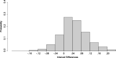
Figure 1: Distribution of experts’ beliefs (group mean) on the difference in success rates between topiramate and control in achieving pain relief at 2 hours in migraine headaches.

2 A full Bayesian solution: Methodology, theory and algorithm

2.1 Summarize external/prior information using an informative prior distribution

Beta distributions are often conventional choices for modeling the prior of the Bernoulli parameter $p_{0}$ or $p_{1}$. They are sufficiently flexible for capturing distributions of different shapes. In particular, we consider four forms of joint beta distributions for the prior of $(p_{0},p_{1})$.

• Independent Beta prior. Joseph, du Berger and Belisle (1997) used independent beta priors to summarize “pre-experimental information” about “two independent binomial parameters” $p_{0}$ and $p_{1}$ as follows: $\pi(p_{0},p_{1})=\pi(p_{0})\pi(p_{1})$ with $\pi(p_{0})\sim\operatorname{BETA}(q_{0},r_{0})$ and $\pi(p_{1})\sim\operatorname{BETA}(q_{1},r_{1})$. Here, $(q_{0},r_{0},q_{1},r_{1})$ are unknown prior parameters (hyperparameters) which can be estimated using the method of moments, following Lee (1992) and Joseph, du Berger and Belisle (1997). Specifically, for our clinical study, the average treatment effect and its standard deviation, $\mu_{d}$ and $\sigma_{d}$, can be obtained (estimated) from the mean and standard deviation of the histogram of Figure 1. Based on previous clinical trials [cf. Silberstein et al. (2004) and Brandes et al. (2004)], the average effectiveness $\mu_{0}$ of Treatment B and its standard deviation $\sigma_{0}$ can also be obtained. We can estimate the prior parameters $(q_{0},r_{0},q_{1},r_{1})$ by solving the equations $\mu_{0}\stackrel{{\scriptstyle\mathrm{set}}}{{=}}\mathrm{E}(p_{0})={q_{0}/{(q_{0}+r_{0})}}$, $\mu_{0}+\mu_{d}\stackrel{{\scriptstyle\mathrm{set}}}{{=}}\mathrm{E}(p_{1})={q_{1}/{(q_{1}+r_{1})}}$, $\sigma_{0}^{2}\stackrel{{\scriptstyle\mathrm{set}}}{{=}}\operatorname{var}(p_{0})={q_{0}r_{0}/\{(q_{0}+r_{0})^{2}(q_{0}+r_{0}+1)\}}$ and $\sigma_{d}^{2}-\sigma_{0}^{2}\stackrel{{\scriptstyle\mathrm{set}}}{{=}}\operatorname{var}(p_{1})=q_{1}r_{1}/\{(q_{1}+r_{1})^{2}(q_{1}+$ $r_{1}+1)\}$.

• Independent hierarchical Beta prior. Gelman et al. [(2004), Chapter 5] suggested that hierarchical priors are more flexible and can avoid “problems of over-fitting” in Bayesian models. We modify their approach to reflect the informative prior in our problem setting with two sets of independent Bernoulli experiments. Specifically, we still model the prior of $(p_{0},p_{1})$ independently with $\pi(p_{0},p_{1})=\pi(p_{0})\pi(p_{1})$, but each $\pi(p_{i})$, for $i=0,1$, assumes two levels of hierarchies as follows:

  $$p_{i}|q_{i},r_{i} \sim \operatorname{BETA}(q_{i},r_{i}),$$

  $$\xi_{i} = \frac{q_{i}}{q_{i}+r_{i}}\sim\operatorname{BETA}(\alpha_{i},\beta_{i})\quad\mbox{and}\quad\eta_{i}=q_{i}+r_{i}\sim\operatorname{GAMMA}(\alpha_{i}+\beta_{i}).$$

  Here, $\xi_{i}$ is the mean and $\eta_{i}$ is the “sample size” of $\operatorname{BETA}(q_{i},r_{i})$, following Gelman et al. (2004), and $\operatorname{GAMMA}(t)$ refers to the standard gamma distribution whose shape parameter is $t$ and scale parameter is 1. Again, we use the method of moments to estimate the unknown parameters in this (hyper) prior distribution. In this case, the first two marginal moments of $p_{i}$ are $\mathrm{E}(p_{i})=\alpha_{i}/(\alpha_{i}+\beta_{i})$ and $\operatorname{var}(p_{i})=\alpha_{i}/\{(\alpha_{i}+\beta_{i})(\alpha_{0}+\beta_{0}+1)\}[\alpha_{i}+\beta_{i}+\int\{(x+1)^{-1}x^{\alpha_{i}+\beta_{i}}e^{-x}/\Gamma(\alpha_{i}+\beta_{i})\}\,dx]$, for $i=0,1$. The prior parameters $(\alpha_{0},\beta_{0},\alpha_{1},\beta_{1})$ are obtained by solving the equations $\mu_{0}\stackrel{{\scriptstyle\mathrm{set}}}{{=}}\mathrm{E}(p_{0})$, $\mu_{0}+\mu_{d}\stackrel{{\scriptstyle\mathrm{set}}}{{=}}\mathrm{E}(p_{1})$, $\sigma_{0}^{2}\stackrel{{\scriptstyle\mathrm{set}}}{{=}}\operatorname{var}(p_{0})$ and $\sigma_{d}^{2}-\sigma_{0}^{2}\stackrel{{\scriptstyle\mathrm{set}}}{{=}}\operatorname{var}(p_{1})$.

• Dependent bivariate Beta (BIBETA) prior. Although most of the analysis in Joseph, du Berger and Belisle (1997) was based on the independent beta prior, a dependent beta prior, with $\pi(p_{0})$ and $\pi(p_{1}|p_{0})=\pi(p_{0},p_{1})/\pi(p_{0})$ both being beta distributions, was considered in a numerical example there. Joseph, du Berger and Belisle (1997) commented that “it is often desirable to allow dependence between $p_{0}$ and $p_{1}$.” This point is particularly relevant to our case study, since almotriptan is used in both groups. However, the constraint $\mathrm{E}(p_{1})=\mathrm{E}(p_{0})$, required in the formulation in Joseph, du Berger and Belisle (1997), does not fit our case. Instead, we use a more flexible bivariate beta distribution (BIBETA), introduced in Olkin and Liu (2003), to model $(p_{0},p_{1})$ in our prior function. This BIBETA distribution ensures that the marginal prior distributions of $p_{0}$ and $p_{1}$ are both beta distributions. More importantly, it also allows modeling the correlation between $p_{0}$ and $p_{1}$ in the range [0,1]. This BIBETA distribution, with parameters $q_{0}$, $q_{1}$ and $r$, has a nice latent structure, that is, $p_{0}={U/(U+W)}$ and $p_{1}={V/(V+W)}$, where $U,V$ and $W$ are standard gamma random variables with respective shape parameters $q_{0},q_{1}$ and $r$. It follows that the joint density (prior distribution) of $p_{0}$ and $p_{1}$ is

  $$\pi(p_{0},p_{1})\propto\frac{p_{0}^{q_{0}-1}p_{1}^{q_{1}-1}(1-p_{0})^{q_{1}+r-1}(1-p_{1})^{q_{0}+r-1}}{(1-p_{0}p_{1})^{q_{0}+q_{1}+r}}.$$

  We obtain the prior parameter values $(q_{0},q_{1},r)$ by the method of moments, solving equations $\mu_{0}\stackrel{{\scriptstyle\mathrm{set}}}{{=}}$ $\mathrm{E}(p_{0})={q_{0}/{(q_{0}+r)}}$, $\mu_{d}\stackrel{{\scriptstyle\mathrm{set}}}{{=}}$ $\mathrm{E}(p_{1}-p_{0})={q_{1}/{(q_{1}+r)}}-{q_{0}/{(q_{0}+r)}}$ and $\sigma_{d}^{2}+\mu_{d}^{2}\stackrel{{\scriptstyle\mathrm{set}}}{{=}}$ $\mathrm{E}(p_{1}-p_{0})^{2}=\{q_{0}(q_{0}+1)\}/\{(q_{0}+r)$ $(q_{0}+r+1)\}+{\{q_{1}(q_{1}+1)\}/\{(q_{1}+r)(q_{1}+r+1)\}}-2_{3}F_{2}(q_{0}+1,q_{1}+1,q_{0}+q_{1}+r;q_{0}+q_{1}+r+1,q_{0}+q_{1}+r+1;1).$ Here ${}_{3}F_{2}(\cdot)$ denotes a hypergeometric function, which can be calculated using the software Mathematica, as mentioned in Olkin and Liu (2003).

• Dependent hierarchical BIBETA prior. We also consider a hierarchical BIBETA prior in which we assign hyperprior distributions on the parameters of the BIBETA distribution:

  $$(p_{0},p_{1})|q_{0},q_{1},r \sim \operatorname{BIBETA}(q_{0},q_{1},r),$$

  $$q_{0} \sim \operatorname{GAMMA}(\alpha_{0}),q_{1}\sim\operatorname{GAMMA}(\alpha_{1})\quad\mbox{and}$$

  $$r \sim \operatorname{GAMMA}(\beta).$$

  The second level of the hyperprior model implies that $\xi_{i}={q_{i}/{(q_{i}+r)}}\sim\operatorname{BETA}(\alpha_{i},$ $\beta)$ and $\eta_{i}=q_{i}+r\sim\operatorname{GAMMA}(\alpha_{i}+\beta)$, for $i$ = 0,1, which matches the conventional parameterization of hierarchical beta priors. This hierarchical BIBETA prior is more flexible than the regular BIBETA distribution. To obtain the prior parameter values $(\alpha_{0},\alpha_{1},\beta)$, we solve equations $\mu_{0}\stackrel{{\scriptstyle\mathrm{set}}}{{=}}\mathrm{E}(p_{0})$, $\mu_{d}\stackrel{{\scriptstyle\mathrm{set}}}{{=}}\mathrm{E}(p_{1}-p_{0})$ and $\sigma_{d}^{2}\stackrel{{\scriptstyle\mathrm{set}}}{{=}}\operatorname{var}(p_{1}-p_{0}).$ Here, the marginal means of $p_{0}$ and $p_{1}$ are simply $\mathrm{E}(p_{0})=\alpha_{0}/(\alpha_{0}+\beta)$ and $\mathrm{E}(p_{1})=\alpha_{1}/(\alpha_{1}+\beta)$. The marginal variance $\operatorname{var}(p_{1}-p_{0})=\mathrm{E}\{\operatorname{var}(p_{1}-p_{0}|q_{0},q_{1},r)\}+\operatorname{var}\{\mathrm{E}(p_{1}-p_{0}|q_{0},q_{1},r)\}$ involves three integrations which can be obtained by numerical integration.

2.2 Summarize trial data of binary outcomes as a likelihood function

For the clinical trial with binary outcomes, the likelihood function of $(p_{0},p_{1})$ is

$$\qquad{\ell}(p_{0},p_{1}|n_{0},{\bar{X}}_{0},n_{1},{\bar{X}}_{1})\propto p_{0}^{n_{0}{\bar{X}}_{0}}p_{1}^{n_{1}{\bar{X}}_{1}}(1-p_{0})^{n_{0}(1-{\bar{X}}_{0})}(1-p_{1})^{n_{1}(1-{\bar{X}}_{1})}.$$ (2)

2.3 Combine prior information and trial data as a posterior distribution

Following the Bayes formula, each of the four prior distributions can be incorporated with the likelihood function (2) to produce a joint posterior distribution of $(p_{0},p_{1})$,

$$\pi(p_{0},p_{1}|n_{0},{\bar{X}}_{0},n_{1},{\bar{X}}_{1})\propto\pi(p_{0},p_{1})\ell(p_{0},p_{1}|n_{0},{\bar{X}}_{0},n_{1},{\bar{X}}_{1}).$$ (3)

The marginal posterior distribution for the parameter of interest $\delta(\equiv p_{1}-p_{0})$ is then

$$\qquad\pi(\delta|n_{0},{\bar{X}}_{0},n_{1},{\bar{X}}_{1})=\int_{\max(0,-\delta)}^{\min(-\delta+1,1)}f(p_{0},p_{0}+\delta|n_{0},{\bar{X}}_{0},n_{1},{\bar{X}}_{1})\,dp_{0},$$ (4)

from which exact Bayesian inferences for $\delta$ can be drawn.

In the case where the prior is modeled by two independent beta distributions, the posterior distribution (3) is simply a product of two independent beta distributions, $\operatorname{BETA}(n_{0}\bar{X}_{0}+q_{0},n_{0}(1-\bar{X}_{0})+r_{0})$ and $\operatorname{BETA}(n_{1}\bar{X}_{1}+q_{1},n_{1}(1-\bar{X}_{1})+r_{1})$. However, in the other three cases both (3) and (4) are not of any known form of distributions and thus are difficult to manipulate. To this end, we propose a Metropolis–Hastings algorithm to simulate random samples from the posterior distributions (3) and (4). See Appendix I [Xie et al. (2013)] for the proposed Metropolis–Hastings algorithm.

The resulting marginal posterior density of $\delta$ in (4) incorporates the prior evidence of expert opinions on the treatment improvement $\delta$ with the evidence from clinical data. The full Bayesian approaches are theoretically sound and should provide a systematic solution to our problem in the Bayesian paradigm. However, as observed in Section 4.2, in the case of a skewed prior, the approaches may lead to the discrepant posterior phenomenon in that the posterior distributions of $\delta$ can yield an estimate that is not between the two estimates derived from the corresponding prior distribution and the likelihood evidence! Further examination suggests that this phenomenon is quite general. See Section 4.2 for details.

3 A frequentist Bayes compromise: A CD approach

In this section we use the so-called confidence distribution (CD) to develop a new approach for incorporating expert opinions with the trial data of binary outcomes. This approach follows frequentist principles and treats parameters as fixed nonrandom values. It provides an attractive alternative to Bayesian methods. In Section 3.1 we provide a definition and a brief review of the CD concept. In Sections 3.2–3.4 we develop the proposed CD approach. This approach can be simply outlined as follows: use a CD to summarize the prior information or expert opinions (Section 3.2), use another CD (often from a likelihood function) to summarize the observed data from the clinical trial (Section 3.3), and then combine these two CDs into one CD (Section 3.4). This combined CD can be used to derive various inferences. Its role in frequentist inference is similar to that of a posterior distribution in Bayesian inference. This development provides yet another example in which a CD can provide useful statistical inference tools for problems where frequentist methods with desirable properties were previously unavailable. Bickel (2006) gives a similar development for normal clinical trials using an objective Bayes argument. The review article by Xie and Singh (2012) contains further discussion.

3.1 A brief review of confidence distribution (CD)

The CD concept is a simple one. For practical purposes, a CD is simply a distribution estimator for a parameter of interest. More specifically, instead of the usual point estimators or interval estimators (i.e., confidence intervals), CD uses a distribution function to estimate the parameter. The development of the CD has a long history; see, for example, Fisher (1930), Neyman (1941) and Lehmann (1993). But its associated inference schemes and applications have not received much attention until recently; see, for example, Efron (1998), Schweder and Hjort (2002, 2003, 2012), Singh, Xie and Strawderman (2001, 2005, 2007), Lawless and Fredette (2005), Tian et al. (2011), Xie, Singh and Strawderman (2011) and Singh and Xie (2012). Although the CD approach is closely related to Fisher’s fiducial approach, as seen in the classical literature, the new CD developments are purely frequentist tools involving no fiducial reasoning. Further discussion of this point as well as the relations between CD-based inference and fiducial and Bayesian inferences can be found in the comprehensive review by Xie and Singh (2012).

The following CD definition is formulated in Schweder and Hjort (2002) and Singh, Xie and Strawderman (2005) under the framework of frequentist inference. Singh, Xie and Strawderman (2005) demonstrated that this new version is consistent with the classical CD definition, and it is easier to use in practice. In the definition, $\theta$ (fixed/nonrandom) is the unknown parameter of interest, $\Theta$ is its parameter space, ${\mathbf{X}}_{n}=(X_{1},\ldots,$ $X_{n})^{T}$ is the sample data set, and $\mathcal{X}$ is the corresponding sample space.

Definition A.

A function $H_{n}(\cdot)=H_{n}({\mathbf{X}}_{n},\cdot)$ on $\mathcal{X}\times\Theta\to[0,1]$ is a confidence distribution (CD) for a parameter $\theta$, if it meets the following two requirements: (R1) For each given ${\mathbf{X}}_{n}\in\mathcal{X}$, $H_{n}(\cdot)$ is a continuous cumulative distribution function; (R2) At the true parameter value $\theta=\theta_{0}$, $H_{n}(\theta_{0})\equiv H_{n}({\mathbf{X}}_{n},\theta_{0})$, as a function of the sample ${\mathbf{X}}_{n}$, follows the uniform distribution $U[0,1]$.

The function $H_{n}(\cdot)$ is an asymptotic confidence distribution (aCD), if the $U[0,1]$ requirement holds only asymptotically, and the continuity requirement on $H_{n}(\cdot)$ is dropped. Also, when it exists, $h_{n}(\theta)=H_{n}^{\prime}(\theta)$ is called a CD density or confidence density.

The CD is a function of both the parameter and the random sample. It is also a sample-dependent distribution function on the parameter space, following requirement R1. Conceptually, it estimates the parameter by a distribution function. As an estimation instrument, it is not much different from a point estimator or a confidence interval. For example, for point estimation, any single point (a real value or a statistic) can, in principle, be an estimate for a parameter, and we often impose additional restrictions to ensure that the point estimator has certain desired properties, such as unbiasedness, consistency, etc. The two requirements in Definition A play roles similar to those restrictions. Specifically, R1 suggests that a sample-dependent distribution function on the parameter space can potentially be used as an estimate for the parameter. The $U[0,1]$ requirement in R2 ensures that the statistical inferences (e.g., point estimates, confidence intervals, $p$-values) derived from the CD have desired frequentist properties.

Like a posterior distribution function, a CD contains a wealth of information for inference. It is a useful device for constructing all types of frequentist statistical inferences, including point estimates, confidence intervals and $p$-values. For instance, it is evident from requirement R2 that intervals obtained from a confidence distribution such as $(H_{n}^{-1}(\alpha_{1}),H_{n}^{-1}(1-\alpha_{2}))$ can always maintain the nominal level of $100(1-\alpha_{1}-\alpha_{2})\%$ for coverage of $\theta$. See Section 4 of Xie and Singh (2012) and references therein for more details. Also, the CD concept is rather general. In fact, recent research has shown that Definition A encompasses a wide range of existing examples, including most examples in the classical development of Fisher’s fiducial distributions, bootstrap distributions, significance functions [$p$-value functions, Fraser (1991)], standardized likelihood functions, and certain Bayesian prior and posterior distributions; see, for example, Schweder and Hjort (2002), Singh, Xie and Strawderman (2005, 2007) and Xie and Singh (2012).

Two examples of CDs which are relevant to the exposition of this paper are provided in Appendix II [Xie et al. (2013)]. Further, Singh, Xie and Strawderman (2005) and Xie, Singh and Strawderman (2011) developed a general method for combining CDs from independent studies, which is utilized in Section 3.4.

3.2 Summarize external/prior information using a CD

A key task in our CD approach in this paper is to construct a CD which summarizes the treatment improvement $\delta$, using only the information obtained prior to the clinical trial. In the following few paragraphs we use a set of modeling arguments to justify that the distribution underlying the histogram in Figure 1 is a CD for the prior information. Some of these arguments are similar to those used in Genest and Zidek (1986) for Bayesian approaches, and our concluded prior CD matches in form the prior distribution suggested by Spiegelhalter, Freedman and Parmar (1994). This match of our prior CD with the commonly used Bayesian prior allows a comparison of the CD approach and the Bayesian approach on an equal footing. Note that what we show here is only one of many possible modeling approaches to achieve our purpose. We will not dwell on this topic since the main goal of the paper is to study and compare inference approaches of incorporating expert opinions with clinical trial data.

Example A.2 in Appendix II [Xie et al. (2013)] shows that an informative prior could be viewed as a CD, provided that a sample space of the prior knowledge or past experiments can be defined. In the same spirit, we assume that the expert opinions are based on past knowledge or experiments about the improvement $\delta$ (the knowledge could be from experience or from similar, or informal, or even virtual experiments, but no actual data are available). This assumption ensures an informative prior and allows us to have a prior CD for the improvement $\delta$. In particular, let ${\mathbf{Y}}_{0}$ be a statistic (with the sample realization $\mathbf{y}_{0}$) that summarizes the information on $\delta$ gathered from past experience or experiments. Let $\hat{\delta}({\mathbf{Y}}_{0})$ be an estimator of $\delta$ and also let $F(t)=P\{\hat{\delta}({\mathbf{Y}}_{0})-\delta\leq t\}$ be the cumulative distribution function of $(\hat{\delta}({\mathbf{Y}}_{0})-\delta)$. We assume for simplicity that $F(t)$ does not involve unknown nuisance parameters or, if it does, that they are replaced by their respective consistent estimates (in this case the development here holds only asymptotically). The prior knowledge then gives rise to the following CD (or asymptotic CD) for $\delta$:

$$H_{0}(\delta)=1-F\bigl{(}\hat{\delta}(\mathbf{y}_{0})-\delta\bigr{)},$$ (5)

since the two requirements in Definition A hold for $H_{0}(\delta)$. For illustration, consider the case in which $\{\hat{\delta}({\mathbf{Y}}_{0})-\delta\}/s_{0}\to N(0,1)$, where $s_{0}^{2}$ is an estimate of $\operatorname{var}(\hat{\delta}({\mathbf{Y}}_{0}))$. In this case, (5) is $H_{0}(\cdot)=\Phi(\{\cdot-\hat{\delta}(\mathbf{y}_{0})\}/s_{0})$. Equivalently, $N(\hat{\delta}(\mathbf{y}_{0}),s_{0}^{2})$ is a distribution estimate of $\delta$.

In practice, the realization $\mathbf{y}_{0}$ of the prior trials is unobserved or only vaguely perceived. We rely on a survey of expert opinions to recover this prior information and $H_{0}(\delta)$, as in our case study in Section 1.1. For simplicity, we assume that the $I$ experts in the survey are randomly selected from a large pool of experts on the subject matter. We also assume that the experts are randomly exposed to some pre-existing experiments or knowledge, which in fact resembles a bootstrapping procedure. Denote by ${\mathbf{Y}}_{i}^{*}$ the summary statistic of the pre-existing knowledge on $\delta$ which the $i$th expert is exposed to and upon which his/her opinion is based. It follows that ${\mathbf{Y}}_{i}^{*}$ is a bootstrap copy of ${\mathbf{Y}}_{0}$. Following Example 2.4 of Singh, Xie and Strawderman (2005), a CD for $\delta$ from the bootstrap sample ${\mathbf{Y}}_{i}^{*}$ is

$$H_{0,i}^{*}(\delta)=1-P\bigl{\{}\hat{\delta}\bigl{(}{\mathbf{Y}}_{i}^{*}\bigr{)}-\hat{\delta}(\mathbf{y}_{0})\leq\hat{\delta}({\mathbf{Y}}_{0})-\delta|{\mathbf{Y}}_{0}\bigr{\}}.$$ (6)

This $H_{0,i}^{*}(\cdot)$ is usually the same as $H_{0}(\cdot)$ with probability 1 under some mild conditions, such as those required for standard bootstrap theory.

However, the function $H_{0,i}^{*}(\delta)$ only summarizes the prior knowledge which the $i$th expert is exposed to. We need to associate it with his/her “reported” opinion in the survey table such as in Table 1. Let us define, from the $i$th row of Table 1, an (empirical) cumulative distribution function

$$H_{0,i}^{**}(\delta)=\sum_{k=1}^{12}g_{i,k}^{**}\mathbf{1}_{(\delta\geq L_{k})},$$

where $100g_{i,k}^{**}$ is the $k$th number reported in the $i$th row of Table 1, $L_{k}$ is the lower bound of the $k$th interval and ${\bf 1}_{(\cdot)}$ is the indicator function. This $H_{0,i}^{**}(\delta)$ is the “reported” distribution for the improvement $\delta$ by the $i$th expert.

In the ideal case, if the “reported” expert opinion faithfully recorded the “true” expert opinion and the “true” expert opinion truly reflects the “true” prior knowledge, $H_{0,i}^{*}(\delta)$ and $H_{0,i}^{**}(\delta)$ would be the same. But, there are often variations in reality. A detailed discussion on how to model such variations is provided in Section 5 as a concluding remark. We proceed with the popular “arithmetic pooling” approach, which is also articulated in Spiegelhalter, Freedman and Parmar (1994). An underlying assumption of arithmetic pooling is that the average of the “observed” expert opinions is an unbiased representation of the “true” prior knowledge. In our case, this is equivalent to assuming the additive error model, $H_{0,i}^{**}(\delta)=H_{0,i}^{*}(\delta)+e_{i}$ such that $I^{-1}\sum_{i=1}^{I}e_{i}\approx 0$ uniformly in $\delta$, where $e_{i}=e_{i}(\delta)$ is defined as the difference between $H_{0,i}^{**}(\delta)$ and $H_{0,i}^{*}(\delta)$ and is viewed as a random error for both the discrepancies between the “true” prior knowledge, the “true” expert opinion and the “reported” opinion of the $i$th expert. Under this error model, where the heterogeneous deviation among experts are “averaged out,” it follows that

$$H_{0}(\delta)\approx I^{-1}\sum_{i=1}^{I}H_{0,i}^{**}(\delta)\approx\sum_{k=1}^{12}\bar{g}_{k}\mathbf{1}_{(\delta\geq L_{k})},$$ (7)

where $100\bar{g}_{k}=100I^{-1}\sum_{i=1}^{I}g_{i,k}^{**}$ are the group means reported in the last row of Table 1. From (7), the (standardized) histogram in Figure 1, that is, $f_{\mathrm{hist}}(\delta)=\sum_{k=1}^{12}$ $\{\bar{g}_{k}/{(L_{k+1}-L_{k})}\}$ $\mathbf{1}_{(L_{k+1}>\delta\geq L_{k})}$, is clearly a suitable approximation for the underlying confidence density function $h_{0}(\delta)=H_{0}^{\prime}(\delta)$. Here, the word “standardized” refers to scaling the histogram so that its area is 1. In our calculations in Section 4, we have used $L_{13}=0.24$ as the upper bound of the $12$th interval.

3.3 Summarize clinical trial data as a CD

The task to summarize the clinical trial results into a CD is relatively easier. The maximum likelihood estimator of $\delta$ is ${\hat{\delta}}={\bar{X}}_{1}-{\bar{X}}_{0}$ with variance $C_{d}^{2}=\operatorname{var}({\hat{\delta}})={{p_{1}(1-p_{1})}/{n_{1}}}+{{p_{0}(1-p_{0})}/{n_{0}}}.$ An estimator of $C_{d}^{2}$ is ${\hat{C}}_{d}^{2}={{{\bar{X}}_{1}(1-{\bar{X}}_{1})}/{n_{1}}}+{{{\bar{X}}_{0}(1-{\bar{X}}_{0})}/{n_{0}}}.$ If both $n_{i}$’s tend to $\infty$, we have ${{({\hat{\delta}}-\delta)}/{{\hat{C}}_{d}}}\to N(0,1)$. Therefore, an asymptotic CD for the parameter $\delta$ from the clinical trial is

$$H_{T}(\delta)=\Phi\bigl{(}{({\delta-{\hat{\delta}}})/{{\hat{C}}_{d}}}\bigr{)}.$$ (8)

In other words, the distribution $N({\hat{\delta}},{\hat{C}}_{d}^{2})$ can be used to estimate $\delta$. An alternative approach is to use the profile likelihood function of $\delta$. Specifically, let $\ell_{\mathrm{prof}}(\delta)$ be the log profile likelihood function of $\delta$, and let $\ell_{n}^{*}(\delta)=\ell_{\mathrm{prof}}(\delta)-\ell_{\mathrm{prof}}(\hat{\delta})$. Following Singh, Xie and Strawderman (2007), we can show that

$$H_{T}(\delta)=\int_{-1}^{\delta}h_{T}(\theta)\,d\theta\qquad\mbox{with }h_{T}(\theta)=\frac{e^{\ell_{n}^{*}(\theta)}}{\int_{-1}^{1}e^{\ell_{n}^{*}(\theta)}\,d\theta}\propto e^{\ell_{\mathrm{prof}}(\delta)}$$ (9)

is an asymptotic CD for $\delta$. The two $H_{T}(\cdot)$ above are asymptotically equivalent when the $n_{i}$’s tend to $\infty$.

3.4 Combine prior information and trial data as a combined CD

We can incorporate the prior CD $H_{0}(\delta)$ with the CD $H_{T}(\delta)$ from the clinical trial using a general CD combination method developed by Singh, Xie and Strawderman (2005). Xie, Singh and Strawderman (2011) showed that this general method and its extension can provide a unifying framework for most information combination methods used in current practice, including both the classical approach of combining $p$-values and the modern model-based (fixed and random effects models) meta-analysis approach. In our context, we are combining two CDs. Specifically, we let $G_{c}(t)=P(g_{c}(U_{1},U_{2})\leq t)$, where $U_{1}$ and $U_{2}$ are independent U$[0,1]$ random variables, and $g_{c}(u_{1},u_{2})$ is a continuous function from $[0,1]\times[0,1]$ to $\mathbb{R}$ which is monotonic (say, increasing) in each coordinate. Then,

$$H^{(c)}(\delta)=G_{c}\bigl{\{}g_{c}\bigl{(}H_{0}(\delta),H_{T}(\delta)\bigr{)}\bigr{\}}$$ (10)

is a combined CD for $\delta$ which contains information from both expert opinions and the clinical trial. One simple choice is

$$g_{c}(u_{1},u_{2})=w_{1}\Phi^{-1}(u_{1})+w_{2}\Phi^{-1}(u_{2}),$$ (11)

with weights $w_{1}=1/{\hat{\sigma}_{d}}$ and $w_{2}=1/\hat{C}_{d}$, where $\hat{\sigma}_{d}$ is an estimate of the standard deviation of $H_{0}(\delta)$ (specifically, $\hat{\sigma}_{d}$ is the standard deviation of the histogram in Figure 1 in our application, and it is also an estimate of the standard deviation of $\hat{\delta}$ in the normal case). In this case, $G_{c}(t)$ can be expressed as $\Phi(t/\{(1/\hat{\sigma}_{d}^{2}+1/\hat{C}_{d}^{2})^{1/2}\})$, and thus gives rise to the following combined CD for $\delta$: $H^{(c)}(\delta)=\Phi(\{\Phi^{-1}(H_{0}(\delta))/\hat{\sigma}_{d}+\Phi^{-1}(H_{T}(\delta))$ $/\hat{C}_{d}\}/\{(1/\hat{\sigma}_{d}^{2}+1/\hat{C}_{d}^{2})^{1/2}\})$.

When both $H_{0}(\delta)$ and $H_{T}(\delta)$ are normal (or asymptotically normal) CDs, the normal combination in (11) is the most efficient in terms of preserving Fisher information. In nonnormal cases, Singh, Xie and Strawderman (2005) studied several choices of the function $g_{c}$ and their Bahadur efficiency. But it remains an open question what choice of $g_{c}$ is most efficient in preserving Fisher information in a general nonnormal setting. Although we use the simple normal combination in (11) in this paper mostly for simplicity, our experience with the numerical studies has shown this combination to be quite adequate in most applications. In fact, in many nonnormal cases, it incurs very little loss of efficiency in terms of preserving Fisher information from both $H_{0}(\delta)$ and $H_{T}(\delta)$.

In a Bayesian approach, it is a conventional practice to fit a prior density curve to the histogram in Figure 1. Although this step is not needed in the proposed CD approach, we may sometimes also fit a density function to $f_{\mathrm{hist}}(\delta)$. For example, we may fit a normal curve to the histogram of Figure 1 by matching its first two moments, say, mean $\hat{\mu}_{d}$ and variance $\hat{\sigma}_{d}^{2}$. In this case, we have a normal CD from the expert opinions $H_{0}(\delta)\approx\Phi((\delta-\hat{\mu}_{d})/\hat{\sigma}_{d})$. Incorporating it with $H_{T}(\delta)$ in (8), we have the combined CD $H^{(c)}(\delta)=\Phi((\delta-\tilde{\delta})/{\tilde{C}_{d}})$ or $N({\tilde{\delta}},\tilde{C}_{d}^{2}),$ where $\tilde{\delta}=({\hat{\delta}}/{\hat{C}}_{d}^{2}+\hat{\mu}_{d}/\hat{\sigma}_{d}^{2})/(1/{\hat{C}}_{d}^{2}+1/\hat{\sigma}_{d}^{2})$ and $\tilde{C}_{d}^{2}=(1/{\hat{C}}_{d}^{2}+1/\hat{\sigma}_{d}^{2})^{-1}.$ This combined CD turns out to be the same as the posterior distribution function obtained from the univariate Bayesian approach described in the Introduction when the normal prior $\pi(\delta)\sim N(\hat{\mu}_{d},\hat{\sigma}_{d}^{2})$ is used. Because Bayes’s formula requires that we know $f(\mathrm{data}|\delta)$ in the univariate Bayesian approach and this conditional density function $f(\mathrm{data}|\delta)$ does not exist in our clinical setting, we have argued that the univariate Bayesian approach is not supported by Bayesian theory. The CD development, interestingly, provides theoretical support for using the posterior distribution $N(\tilde{\delta},\tilde{C}_{d}^{2})$ from a non-Bayesian point of view if the prior distribution of expert opinions can be approximated by a normal distribution. In this case, the univariate Bayesian approach can also produce a result that “makes sense,” and practically we can use either the CD approach or the univariate Bayesian approach. But this statement is not true in general.

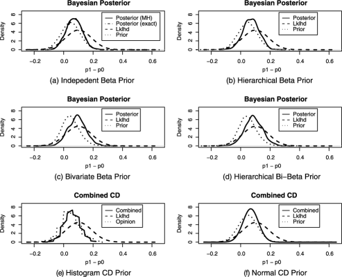
Figure 2: Outcomes of data analysis from the migraine pain data.

Table 2: Numerical results from incorporating expert opinions on PR2 (summarized in Figure 1) with clinical data on PR2: mode, median, mean, $I_{80\%}$, $I_{90\%}$ and $I_{95\%}$ of the marginal prior, (normalized) profile likelihood function and marginal posterior of the parameter $\delta$. Here, $I_{80\%}$, $I_{90\%}$ and $I_{95\%}$ denote the interval [$100\alpha$%-tile, $100(1-\alpha)$%-tile] for $\alpha=10\%$, $5\%$ and $2.5\%$, respectively. Included in the comparison are four full Bayesian approaches and two approaches based on confidence distributions (CDs)

		Mode	Median	Mean	$\bolds{I_{80\%}}$	$\bolds{I_{90\%}}$	$\bolds{I_{95\%}}$
Bayesian approaches
Ind Beta prior	Prior	0.049	0.047	0.048	$-0.037\ 0.130$	$-0.060\ 0.153$	$-0.080\ 0.173$
	Likelihood	0.104	0.104	0.103	$-0.007\ 0.214$	$-0.043\ 0.251$	$-0.062\ 0.269$
	Posterior	0.069	0.070	0.071	$0.000\ 0.138$	$-0.015\ 0.156$	$-0.029\ 0.174$
Hierarchical	Prior	0.048	0.047	0.048	$-0.036\ 0.130$	$-0.059\ 0.154$	$-0.080\ 0.175$
Beta prior	Likelihood	0.104	0.104	0.103	$-0.007\ 0.214$	$-0.043\ 0.251$	$-0.062\ 0.269$
	Posterior	0.082	0.071	0.070	$0.000\ 0.143$	$-0.021\ 0.159$	$-0.037\ 0.171$
Bi-Beta prior	Prior	0.040	0.044	0.048	$-0.029\ 0.125$	$-0.050\ 0.151$	$-0.069\ 0.174$
	Likelihood	0.104	0.104	0.103	$-0.007\ 0.214$	$-0.043\ 0.251$	$-0.062\ 0.269$
	Posterior	0.093	0.091	0.091	$0.015\ 0.165$	$-0.004\ 0.190$	$-0.025\ 0.209$
Hierarchical	Prior	0.043	0.045	0.048	$-0.028\ 0.127$	$-0.049\ 0.154$	$-0.068\ 0.178$
Bi-Beta prior	Likelihood	0.104	0.104	0.103	$-0.007\ 0.214$	$-0.043\ 0.251$	$-0.062\ 0.269$
	Posterior	0.082	0.086	0.087	$0.013\ 0.162$	$-0.01\ \phantom{0}0.189$	$-0.031\ 0.207$
CD approaches
CD with	Prior CD	0.020	0.060	0.048	$-0.023\ 0.142$	$-0.068\ 0.145$	$-0.070\ 0.182$
histogram prior	Likelihood	0.104	0.104	0.103	$-0.007\ 0.214$	$-0.043\ 0.251$	$-0.062\ 0.269$
	Comb. CD	0.060	0.065	0.058	$0.013\ 0.141$	$-0.022\ 0.145$	$-0.025\ 0.182$
CD with	Prior CD	0.048	0.048	0.048	$-0.034\ 0.132$	$-0.058\ 0.156$	$-0.078\ 0.177$
normal prior	Likelihood	0.104	0.104	0.103	$-0.007\ 0.214$	$-0.043\ 0.251$	$-0.062\ 0.269$
	Comb. CD	0.068	0.068	0.068	$0.001\ 0.135$	$-0.018\ 0.154$	$-0.035\ 0.171$

4 Application: Numerical results and comparisons

We now provide numerical studies to illustrate and compare the Bayesian and CD approaches discussed in Sections 2 and 3. In Section 4.1 we focus on the data from the migraine pain study outlined in Section 1.1. In Section 4.2 we simulate a skewed distribution of expert opinions and combine the simulated prior information with the clinical trial data.

4.1 Normal priors: A case study of the migraine pain data

For the outcome PR2, the clinical data report that 31 out of 68 patients in the control group and 33 out of 59 patients in the treatment group achieved pain relief at 2 hours. Our goal is to incorporate the expert inputs reported in Figure 1 with these observed outcomes.

We apply the full Bayesian approach described in Section 2 to analyze the PR2 data, using each of the four beta priors for $(p_{0},p_{1})$. The numerical results are reported in Figures 2(a)–(d) and also in the first 12 rows of Table 2. The dotted lines in Figures 2(a)–(d) indicate the marginal prior density functions, and the dashed lines indicate the (standardized) profile likelihood function of $\delta$ based only on the clinical trial data. The solid lines in Figures 2(a)–(d) are the marginal posterior distributions of $\delta$. They are obtained by using the density estimation function density($\cdot$) in the R software and from 1000 Metropolis–Hasting samples of $\delta^{*}=p_{1}^{*}-p_{0}^{*}$. In each case and for each of the 1000 replications, the Metropolis–Hastings algorithm is iterated $t=25\mbox{,}000$ times (burn-in). The acceptance rates are on average $0.0379$, $0.0381$, $0.0480$ and $0.0485$, respectively, in (a) to (d). For the independent beta prior, the exact formula of the posterior distribution is available, and it is plotted in Figure 2(a) as the dash-dot broken curve (it is barely visible in the plot, since it is almost identical to the solid curve). The close agreement of these two curves for the posterior distribution indicates that the MCMC chain of the Metropolis–Hastings algorithm has generally converged with $t=25\mbox{,}000$ in this case.

In applying the CD approach, we use both the raw histogram in Figure 1 and the $N(\hat{\mu}_{d},\hat{\sigma}_{d}^{2})$ distribution to approximate the prior CD of expert opinions. Figures 2(e)–(f) and the last six rows of Table 2 contain numerical results. The dotted lines in Figures 2(e)–(f) indicate the prior CDs, the dashed lines indicate the profile likelihood function of $\delta$ based only on the clinical trial data, and the solid lines are for the combined CDs for $\delta$.

In this particular example, all six approaches (four Bayesian and two CD approaches) seem to yield similar posterior or combined CD functions, and thus similar statistical inferences, regardless of which approach is used. Although the six marginal posterior or combined CD distributions are slightly different from one another, the difference appears to all fall within the expected estimation error of the density curves. This result is not surprising, since, although skewed, the degree of skewness of the histogram in Figure 1 does not appear to be great enough to render the normal approximation invalid. In fact, in this case, such a result is expected to hold if the central limit theory is in place for the clinical data of binary outcomes. It is worth noting here that the Bayesian approach implemented through an MCMC method is more demanding computationally.

4.2 Skewed priors: A simulation study

The outcome in the previous subsection begs the question of whether there would be a significant difference among the approaches if the distribution of expert opinions were unambiguously skewed, so that the normal approximation is clearly not valid. Conventional wisdom suggests that full Bayesian approaches based on beta priors, though computationally more intensive, would have advantages due to their flexibility in capturing distributions of various shapes. The CD approaches, allowing skewed priors, may also work. However, the numerical results reveal a surprising finding in the full Bayesian approaches.

In this simulation study, we again use the observed clinical data on PR2, but replace Table 1 and Figure 1 of expert opinions with their simulated counterparts, assuming that the underlying prior distribution function of $(p_{0},p_{1})$ is a bivariate beta distribution, $\operatorname{BIBETA}(6,20,2)$. The marginal means of the $\operatorname{BIBETA}(6,20,2)$ distribution are $\mathrm{E}p_{0}=6/(6+2)=0.75$ and $\mathrm{E}p_{1}=20/(20+2)\approx 0.90$. Thus, the simulated prior represents a treatment effect improvement on average about 75% to 90%, which are similar to those of the real trial in Section 4.1. Specifically, we simulate responses of 100 patients for each of the 11 experts from $\operatorname{BIBETA}(6,20,2)$, tally the results in the format of Table 1 (not shown), and then plot them as a histogram in Figure 3. For a direct visual comparison, Figure 3 includes the curve of the $\operatorname{BIBETA}(6,20,2)$ density. Also plotted in Figure 3 is, as a common approach to fitting a skewed distribution, the following fitted log-normal density $\phi(\{\log(\delta)-\log(\hat{\mu}_{d}-c)\}/\{1+\hat{\sigma}_{d}^{2}/(\hat{\mu}_{d}-c)^{2}\}^{1/2}-\frac{1}{2}\sqrt{1+\hat{\sigma}_{d}^{2}/(\hat{\mu}_{d}-c)^{2}})/\{\delta(1+\hat{\sigma}_{d}^{2}/(\hat{\mu}_{d}-c)^{2})^{1/2}\}$. Here, $\hat{\mu}_{d}$ and $\hat{\sigma}_{d}$ are the mean and the standard deviation computed from the histogram, and $c$ is a constant used to capture the shift of the log-normal distribution from $0$.

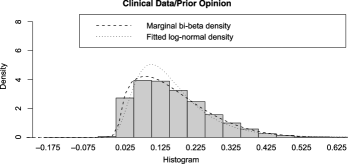
Figure 3: Simulated prior distribution of $\delta=p_{1}-p_{0}$ using $\operatorname{BIBETA}(6,20,2)$ distribution.

We apply the same four full Bayesian approaches used in Section 4.1 to incorporate the simulated expert opinions represented in Figure 3 with the clinical trial data on PR2. The four sets of prior parameters used in these four approaches are $(q_{0},r_{0},q_{1},r_{1})=(14.66,4.88,46.81,4.68)$, $(\alpha_{0},\beta_{0},\alpha_{1},\beta_{1})=\break(30.19,10.06,96.43,9.43)$, $(q_{0},q_{1},r)=(6,20,2)$ and $(\alpha_{0},\alpha_{1},\beta)=(17.88,$ $59.60,$ $5.96)$, respectively. In the third approach, we directly use the true set of prior parameters $(q_{0},q_{1},r)=(6,20,2)$; in the other three, the prior parameters are obtained by the method of moments outlined in Section 2. In the simulation example, the Metropolis–Hasting algorithm is again iterated $t=25,000$ times (burn-in), and it is repeated 1000 times to obtain 1000 independent Metropolis–Hasting samples of $(p_{0}^{*},p_{1}^{*})$ in each case. The acceptance rates are on average $0.0019$, $0.0027$, $0.0057$ and $0.0036$, respectively.

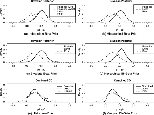
Figure 4: Outcomes of data analysis from simulated data with a skewed prior.

Table 3: Numerical results from incorporating the simulated expert opinions (summarized in Figure 3) with clinical data on PR2: the mode, median, mean, $I_{80\%}$, $I_{90\%}$ and $I_{95\%}$ of the marginal prior, (normalized) profile likelihood function, and marginal posteriorof the parameter $\delta$. Here, $I_{80\%}$, $I_{90\%}$ and $I_{95\%}$ denote the interval [$100\alpha$%-tile, $100(1-\alpha)$%-tile] for $\alpha=10\%$, $5\%$ and $2.5\%$, respectively. The prior parametersin the four full Bayesian approaches are $(q_{0},r_{0},q_{1},r_{1})=(14.66,4.88,46.81,4.68)$, $(\alpha_{0},\beta_{0},\alpha_{1},\beta_{1})=(30.19,10.06,96.43,9.43)$, $(q_{0},q_{1},r)=(6,20,2)$ and$(\alpha_{0},\alpha_{1},\beta)=(17.88,59.60,5.96)$, respectively

		Mode	Median	Mean	$\bolds{I_{80\%}}$	$\bolds{I_{90\%}}$	$\bolds{I_{95\%}}$
Bayesian approaches
Independent	Prior	0.128	0.153	0.159	$0.033\ 0.297$	$0.003\ 0.340$	$-0.023\ 0.379$
Beta prior	Likelihood	0.104	0.104	0.103	$-0.007\ 0.214$	$-0.043\ 0.251$	$-0.062\ 0.269$
	Posterior	0.211	0.212	0.212	$0.120\ 0.306$	$0.089\ 0.330$	$0.066\ 0.346$
Hierarchical	Prior	0.145	0.152	0.159	$0.031\ 0.295$	$-0.001\ 0.337$	$-0.027\ 0.375$
Beta prior	Likelihood	0.104	0.104	0.103	$-0.007\ 0.214$	$-0.043\ 0.251$	$-0.062\ 0.269$
	Posterior	0.214	0.212	0.212	$0.122\ 0.302$	$0.094\ 0.329$	$0.078\ 0.348$
Independent	Prior	0.095	0.140	0.159	$0.042\ 0.306$	$0.027\ 0.360$	$0.017\ 0.407$
Bi-Beta prior	Likelihood	0.104	0.104	0.103	$-0.007\ 0.214$	$-0.043\ 0.251$	$-0.062\ 0.269$
	Posterior	0.202	0.203	0.201	$0.112\ 0.288$	$0.084\ 0.315$	$0.061\ 0.339$
Hierarchical	Prior	0.120	0.146	0.159	$0.056\ 0.281$	$0.039\ 0.326$	$0.028\ 0.366$
Bi-Beta prior	Likelihood	0.104	0.104	0.103	$-0.007\ 0.214$	$-0.043\ 0.251$	$-0.062\ 0.269$
	Posterior	0.232	0.225	0.222	$0.138\ 0.305$	$0.116\ 0.329$	$0.101\ 0.340$
CD approaches
CD with	Prior CD	0.075	0.125	0.159	$0.025\ 0.275$	$-0.025\ 0.325$	$-0.025\ 0.375$
histogram	Likelihood	0.104	0.104	0.103	$-0.007\ 0.214$	$-0.043\ 0.251$	$-0.062\ 0.269$
prior	Comb. CD	0.100	0.110	0.118	$0.035\ 0.200$	$0.000\ 0.225$	$-0.005\ 0.250$
CD with	Prior CD	0.095	0.140	0.159	$0.042\ 0.306$	$0.027\ 0.360$	$0.017\ 0.407$
marginal	Likelihood	0.104	0.104	0.103	$-0.007\ 0.214$	$-0.043\ 0.251$	$-0.062\ 0.269$
Bi-Beta prior	Comb. CD	0.099	0.099	0.119	$0.026\ 0.191$	$0.007\ 0.209$	$-0.011\ 0.246$

We also apply two CD combination approaches to incorporate the simulated expert opinions in Figure 3 with the clinical trial data on PR2. Similar to that in Section 4, the first CD approach directly uses the raw histogram in Figure 3. The second CD approach, in order to have a direct comparison with the Bayesian approach using the underlying prior $\operatorname{BIBETA}(6,20,2)$, combines the underlying marginal density function of $\delta$ with the CD from the clinical trial data. Of course, in reality we do not know the underlying prior distribution or the underlying marginal density function of $\delta$. Thus, the second CD approach has only theoretical value. Without relying on the underlying CD prior, we also consider the CD approach which combines the fitted log-normal distribution in Figure 3 with the CD from the clinical trial data. However, since the log-normal curve is evidently a poor fit for the histogram in Figure 3, the result for this CD approach, though not too far off, does not seem well justified and is thus omitted.

Figures 4(a)–(d) show the results on the improvement $\delta$ using the full Bayesian approaches, and Figures 4(e)–(f) show the results using the CD combination approaches. Figure 4 adopts the same notation and symbols used in Figure 2. Again, for the independent beta prior, the posterior density from the algorithm closely matches the one using its exact formula (dashed-dotted line), indicating that the MCMC chain of the Metropolis–Hasting algorithm has generally converged in this case. Also, we report in Table 3 the numerical results from the six approaches: the mode, median, mean and confidence/credible intervals of the marginal priors, the profile likelihood function and the marginal posteriors of $\delta$.

The CD approaches perform exactly as anticipated. However, examining the modes of the three curves in each of Figures 4(a)–(d), we notice that the mode of the marginal posterior distribution (solid curve) lies to the right of the peaks of both the marginal prior distribution (dotted curve) and the profile likelihood function (dashed curve). The numerical results in Table 3 also confirm that the mode, median and mean of the marginal posterior distributions of $\delta$ from all four full Bayesian approaches are much larger than their counterparts from the corresponding marginal priors and profile likelihood functions. This discrepant posterior phenomenon is counterintuitive! For instance, if we use the means as our point estimators, we would report from Figure 4(c) that the experts suggest about $15.9\%$ improvement and the clinical evidence suggests about $10.3\%$ improvement but, incorporating them together, the overall estimator of the treatment effect is $20.1\%$, which is bigger than either that reported by the experts or that suggested by the clinical data. This result is certainly not easy to explain to clinicians or general practitioners of statistics. In any event, it seems worthwhile to investigate further and see what ramifications this intriguing phenomenon may have.

To further examine the phenomenon, we compare the percentiles of the marginal priors, the profile likelihood function and the marginal posterior distributions of the treatment effect $\delta$ in Table 3. In each of the four Bayesian approaches, the 95% posterior credible interval lies inside the corresponding 95% interval from the prior and has substantial overlap with the corresponding 95% interval from the profile likelihood. But this is not always the case at the 80% and 90% levels, where several posterior credible intervals do not lie within the boundaries of the corresponding intervals from the priors and the likelihood functions. The outcome of whether the posterior credible interval lies within the boundaries of the other two depends on the choice of the credible level. Thus, using credible intervals as our primary inferential instrument cannot completely avoid the discrepant posterior phenomenon either.

To better understand this phenomenon, we plot in Figures 5(a)–(d) the contours of the joint prior distribution $\pi(p_{0},p_{1})$, the likelihood function of $(p_{0},p_{1})$ and the joint posterior distribution of $(p_{0},p_{1})$ for each of the four full Bayesian approaches. We show that certain projections of Figures 5(a)–(d) lead to the marginal distributions and plots in Figures 4(a)–(d). As marked in Figure 5, the center (mode) of each contour plot is on a line $\delta=p_{1}-p_{0}$ (or $p_{1}=p_{0}+\delta$). Varying $\delta$ in $\delta=p_{1}-p_{0}$ produces a family of parallel lines, all making a $45^{o}$ angle with the horizontal axis. The projections of the three distributions along these parallel lines onto the interval of possible values of $\delta$, $-1<\delta<1$, lead to the plots of marginal distributions in Figures 4(a)–(d). The yellow curves in (a) are a posterior contour plot from the exact formula. Although the contour plots of the posterior distributions sit between those of the prior distributions and the likelihood function, their projected peaks (modes) are more to the upper-left than those of the marginal priors and the profile likelihood function. Further investigation indicates that this is a genuine mathematical phenomenon which holds for all four Bayesian approaches and not merely an aberration due to some special circumstances. In fact, when the center (mode) of a posterior distribution is not in the interval joining the two centers (modes) of the joint prior and likelihood functions, as is often the case with skewed distributions (and even sometimes with nonskewed distributions), there always exists a linear direction, say, $ap_{0}+bp_{1}$ with some coefficients a and b, along which the marginal posterior fails to fall between the marginal prior and likelihood functions of the same parameter. Reparametrization, if done carefully, such as considering joint distribution of $(\delta,\theta)=(p_{1}-p_{0},p_{1}+p_{0})$ or others, may sometimes help hide the discrepant posterior phenomenon on the $\delta$ direction, but cannot eliminate it systematically. We have found no discussion of such a geometric finding on marginalization in the Bayesian literature. See further discussion in Section 5.

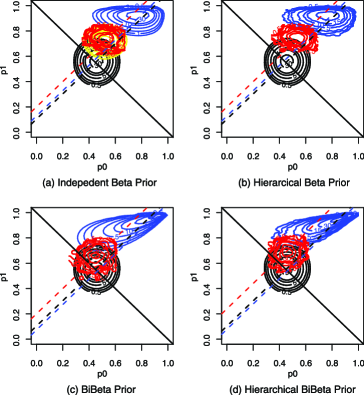
Figure 5: Contour plots: joint prior distribution (in blue), joint likelihood function (in black) and estimated posterior distribution (in red) of $(p_{0},p_{1})$. These two-dimensional distributions are projected along the $45^{o}$ lines of $\delta=p_{1}-p_{0}$ onto the interval of possible values of $\delta$, $-1<\delta<1$, leading to Figures 4(a)–(d). The yellow curves in (a) are a posterior contour plot from the exact formula.

5 Conclusions and additional remarks

To incorporate expert opinions in the analysis of a clinical trial with binary outcomes in a meaningful way, we have developed and studied several bivariate full Bayesian approaches as well as a CD approach. We show that both the Bayesian and the proposed CD approaches may provide viable solutions. Although the paper focuses on expert opinions in pharmaceutical studies, the methodologies developed here can be applied to incorporating other types of priors or external information, for example, historical knowledge. These methodologies should also be useful in many other fields, including finance, social science studies and even homeland security, where prior knowledge, expert opinions and historical information are much valued and need to be incorporated with observed data in an effective and justifiable manner.

In this paper we have examined and compared both Bayesian and CD approaches. Although there does not exist the usual theoretical platform for a direct comparison on efficiency or lengths of intervals, the comparison can be summarized in three aspects: empirical results, computational effort and theoretical consideration. The empirical findings from Figure 2 show that, as long as the histogram of the expert opinions can be well approximated by a normal distribution, all approaches considered in this paper perform comparably, in terms of the posterior distribution or the combined CD and their corresponding inferences. However, if the histogram is skewed, the full Bayesian approach may produce the discrepant posterior phenomenon, which is difficult to avoid in theory and difficult to explain in applications. The CD approach avoids such a phenomenon.

In terms of the computational effort, the bivariate full Bayesian approach is demanding since it requires running a large-scale simulation using an MCMC algorithm, while the proposed CD approach is both explicit and straightforward to compute. In addition, the CD approach can directly incorporate the histogram of expert opinions without an additional effort of curve fitting.

Theoretically, since it is not possible to find a “marginal” likelihood of $\delta$ [i.e., a conditional density function $f(\mathrm{data}|\delta)$], any univariate Bayesian approach focusing on the parameter of interest $\delta$ is not supported by Bayesian theory. A full Bayesian solution is to jointly model $(p_{0},p_{1})$ [or a reparameterization of the pair $(p_{0},p_{1})$] and, subsequently, make inferences using the marginal posterior of $\delta$. The full Bayesian approaches developed in the paper follow exactly this procedure and are theoretically sound. The proposed CD approach is developed strictly under the frequentist paradigm and is also theoretically sound. Unlike the full Bayesian approaches, the CD approach can focus directly on the parameter of interest $\delta$ without the additional burden of modeling other parameters or the correlation between $p_{0}$ and $p_{1}$, and thus appears to have some advantage in this application.

A surprising finding in this research is the discrepant posterior phenomenon occurring in the full Bayesian approaches under skewed priors. Although it may be mitigated if the prior is only slightly skewed or is in accordance with the likelihood function, the phenomenon is intrinsically mathematical. How much skewness is required to produce the phenomenon depends on all elements involved, including shapes and locations of both the likelihood and the prior. The reactions to this phenomenon we have encountered thus far fall roughly into two groups. One group views the discrepant posterior as a mathematical truth and, if one has faith in the choice of the prior, one should proceed to make inference using this marginal posterior, even though the outcome is counterintuitive. The other worries about the counterintuitive result and would try to find alternative approaches of a good operating characteristic for the particular problem at hand, even at the cost of abandoning the mathematically solid full Bayesian approach in favor of less rigorous approaches such as the univariate Bayesian approach described in Section 1. In any case, the lesson learned from the Bayesian analysis here is that the choice of the prior really matters and it needs to be in some agreement with the likelihood function, which is similar in spirit to what was referred to as “model dependent” in Berger (2006). We also consider this a manifestation of an inherent difficulty in modeling accurately the joint effects of the two treatments as reflected in $p_{0}$ and $p_{1}$ and their correlation. This difficulty illustrates again the complexity of the practice of incorporating external information in trials with binary outcomes.

The discrepant posterior phenomenon is caused by “marginalization,” but it is different from the “marginalization paradox” discussed in Dawid, Stone and Zidek (1973) and Berger (2006). In particular, the marginalization paradox in Dawid, Stone and Zidek (1973) refers to the phenomenon that the marginal posterior of $\pi(\theta|\mathrm{data})$ obtained from the joint prior $\pi(\theta,\phi)$ and its full model $f(\mathrm{data}|\theta,\phi)$ can sometimes be quite different (“incoherent”) from the posterior $\pi(\theta|\mathrm{data})$ obtained by applying the Bayes formula directly to its marginal prior $\pi(\theta)$ and marginal model $f(\mathrm{data}|\theta)$, even though the marginal prior $\pi(\theta)$ and marginal model $f(\mathrm{data}|\theta)$ are consistent (“coherent”) with the joint prior $\pi(\theta,\phi)$ and the full model $f(\mathrm{data}|\theta,\phi)$. Here, $\phi$ represents nuisance parameters. This paradox is different from what we observed here. In our example, it is not possible to have the marginal model $f(\mathrm{data}|\theta)$, and the discrepant posterior phenomenon in the full Bayesian approach is that the estimate derived from the marginal posterior $\pi(\theta|\mathrm{data})$ may not be between the estimates from the marginal prior $\pi(\theta)$ and the profile likelihood function $\ell(\theta|\mathrm{data})$. This is counterintuitive in practical applications.

It is worth noting that the discussion and implications of the discrepant posterior phenomenon extend beyond the setting of binary outcomes to any multivariate setting involving skewed distributions. As long as the center (mode) of a posterior distribution is not in the interval joining the centers (modes) of the joint prior and the likelihood function, there always exists a direction along which the center (mode) of the marginal posterior fails to fall between the centers (modes) of marginal prior and the profile likelihood function. This phenomenon has implications in the general practice of Bayesian analysis. For instance, many researchers in machine learning and other fields routinely draw conclusions solely based on marginal posterior distributions without checking (or it is very difficult to check) the validity of such conclusions. The discrepant posterior phenomenon suggests that further care is needed.

Many methods have been introduced to model “reported” expert opinions, account for their potential errors and heterogeneity, and subsequently pool them; see Genest and Zidek (1986) for an excellent review of this topic. In particular, Spiegelhalter, Freedman and Parmar (1994) described “arithmetic and logarithm pooling” as the “two simplest methods” for pooling expert opinions, and articulated a “strong preference” “for arithmetic pooling to obtain an estimated opinion of a typical participating clinician.” The underlying assumption of arithmetic pooling is that the average of the “observed” expert opinions is an unbiased representation of the “true” prior knowledge. This assumption naturally facilitates the additive error model used in Section 3.2 for summarizing “reported” expert opinions in a CD. Clearly, the modeling principle and development we used to summarize the expert opinions in a CD are similar in spirit to those discussed in Genest and Zidek (1986) and Spiegelhalter, Freedman and Parmar (1994) for Bayesian approaches.

The modeling framework developed in Section 3.2 is sufficiently flexible and can be modified to accommodate various ways of aggregating expert opinions. In particular, it can incorporate weighting schemes to develop a robust method against extreme expert opinions, introduce additional terms to reflect biased opinions or additional uncertainties, or use the geometric mean as a way to pool the expert opinions. Some of these extensions (e.g., the robust method) by themselves could be attractive choices to produce priors in the context of traditional Bayesian approaches. Due to space limitations, we will not pursue these extensions in this paper.

In a different direction, we have also considered modeling the survey data of expert opinions using a traditional random effects approach. In such a model, we provide a regression model for the responses of the 100 “virtual patients” of each expert (as described in Section 1.1) and add a random effect term to account for the expert-to-expert variation. However, it seems nontrivial to overcome the technical difficulty in making the modeling process free of the number (100) of “virtual patients.” In fact, this difficulty led us to the bootstrap argument in Section 3.2, in which we mimic a potential model of expert exposure to pre-existing experiments. Clearly, there remain many challenging issues in modeling the survey data of expert opinions, even for the seemingly simple binary setting.

References

- Berger (2006) {barticle}[mr] \bauthor\bsnmBerger, \bfnmJames\binitsJ. (\byear2006). \btitleThe case for objective Bayesian analysis. \bjournalBayesian Anal. \bvolume1 \bpages385–402 (electronic). \bidmr=2221271 \bptnotecheck related\bptokimsref \endbibitem
- Berry and Stangl (1996) {bbook}[auto:STB—2012/09/04—06:46:48] \bauthor\bsnmBerry, \bfnmD. A.\binitsD. A. and \bauthor\bsnmStangl, \bfnmD.\binitsD. (\byear1996). \btitleBayesian Biostatistics. \bpublisherDekker, \blocationNew York. \bptokimsref \endbibitem
- Bickel (2006) {bmisc}[auto:STB—2012/09/04—06:46:48] \bauthor\bsnmBickel, \bfnmD. R.\binitsD. R. (\byear2006). \bhowpublishedIncorporating expert knowledge into frequentist inference by combining generalized confidence distributions. Unpublished manuscript. \bptokimsref \endbibitem
- Boos and Monahan (1986) {barticle}[auto:STB—2012/09/04—06:46:48] \bauthor\bsnmBoos, \bfnmD. D.\binitsD. D. and \bauthor\bsnmMonahan, \bfnmJ. F.\binitsJ. F. (\byear1986). \btitleBootstrap methods using prior information. \bjournalBiometrika \bvolume73 \bpages77–83. \bptokimsref \endbibitem
- Brandes et al. (2004) {barticle}[pbm] \bauthor\bsnmBrandes, \bfnmJan Lewis\binitsJ. L., \bauthor\bsnmSaper, \bfnmJoel R.\binitsJ. R., \bauthor\bsnmDiamond, \bfnmMerle\binitsM., \bauthor\bsnmCouch, \bfnmJames R.\binitsJ. R., \bauthor\bsnmLewis, \bfnmDonald W.\binitsD. W., \bauthor\bsnmSchmitt, \bfnmJennifer\binitsJ., \bauthor\bsnmNeto, \bfnmWalter\binitsW., \bauthor\bsnmSchwabe, \bfnmStefan\binitsS. and \bauthor\bsnmJacobs, \bfnmDavid\binitsD. (\byear2004). \btitleTopiramate for migraine prevention: A randomized controlled trial. \bjournalJAMA \bvolume291 \bpages965–973. \biddoi=10.1001/jama.291.8.965, issn=1538-3598, pii=291/8/965, pmid=14982912 \bptokimsref \endbibitem
- Carlin and Louis (2009) {bbook}[mr] \bauthor\bsnmCarlin, \bfnmBradley P.\binitsB. P. and \bauthor\bsnmLouis, \bfnmThomas A.\binitsT. A. (\byear2009). \btitleBayesian Methods for Data Analysis, \bedition3rd ed. \bpublisherCRC Press, \blocationBoca Raton, FL. \bidmr=2442364 \bptokimsref \endbibitem
- Dawid, Stone and Zidek (1973) {barticle}[mr] \bauthor\bsnmDawid, \bfnmA. P.\binitsA. P., \bauthor\bsnmStone, \bfnmM.\binitsM. and \bauthor\bsnmZidek, \bfnmJ. V.\binitsJ. V. (\byear1973). \btitleMarginalization paradoxes in Bayesian and structural inference. \bjournalJ. Roy. Statist. Soc. Ser. B \bvolume35 \bpages189–233. \bidissn=0035-9246, mr=0365805 \bptnotecheck related\bptokimsref \endbibitem
- Efron (1986) {barticle}[auto:STB—2012/09/04—06:46:48] \bauthor\bsnmEfron, \bfnmB.\binitsB. (\byear1986). \btitleWhy isn’t everyone a Bayesian? \bjournalAmer. Statist. \bvolume40 \bpages1–11. \bidmr=0828575 \bptokimsref \endbibitem
- Efron (1998) {barticle}[mr] \bauthor\bsnmEfron, \bfnmBradley\binitsB. (\byear1998). \btitleR. A. Fisher in the 21st century (invited paper presented at the 1996 R. A. Fisher Lecture). \bjournalStatist. Sci. \bvolume13 \bpages95–122. \biddoi=10.1214/ss/1028905930, issn=0883-4237, mr=1647499 \bptnotecheck related\bptokimsref \endbibitem
- Fisher (1930) {barticle}[auto:STB—2012/09/04—06:46:48] \bauthor\bsnmFisher, \bfnmR. A.\binitsR. A. (\byear1930). \btitleInverse probability. \bjournalProc. Cambridge Philos. Soc. \bvolume26 \bpages528–535. \bptokimsref \endbibitem
- Fraser (1991) {barticle}[mr] \bauthor\bsnmFraser, \bfnmD. A. S.\binitsD. A. S. (\byear1991). \btitleStatistical inference: Likelihood to significance. \bjournalJ. Amer. Statist. Assoc. \bvolume86 \bpages258–265. \bidissn=0162-1459, mr=1137116 \bptokimsref \endbibitem
- Gelman et al. (2004) {bbook}[mr] \bauthor\bsnmGelman, \bfnmAndrew\binitsA., \bauthor\bsnmCarlin, \bfnmJohn B.\binitsJ. B., \bauthor\bsnmStern, \bfnmHal S.\binitsH. S. and \bauthor\bsnmRubin, \bfnmDonald B.\binitsD. B. (\byear2004). \btitleBayesian Data Analysis, \bedition2nd ed. \bpublisherChapman & Hall/CRC, \blocationBoca Raton, FL. \bidmr=2027492 \bptokimsref \endbibitem
- Genest and Zidek (1986) {barticle}[mr] \bauthor\bsnmGenest, \bfnmChristian\binitsC. and \bauthor\bsnmZidek, \bfnmJames V.\binitsJ. V. (\byear1986). \btitleCombining probability distributions: A critique and an annotated bibliography. \bjournalStatist. Sci. \bvolume1 \bpages114–148. \bidissn=0883-4237, mr=0833278 \bptnotecheck related\bptokimsref \endbibitem
- Joseph, du Berger and Bélisle (1997) {barticle}[pbm] \bauthor\bsnmJoseph, \bfnmL.\binitsL., \bauthor\bparticledu \bsnmBerger, \bfnmR.\binitsR. and \bauthor\bsnmBélisle, \bfnmP.\binitsP. (\byear1997). \btitleBayesian and mixed Bayesian/likelihood criteria for sample size determination. \bjournalStat. Med. \bvolume16 \bpages769–781. \bidissn=0277-6715, pii=10.1002/(SICI)1097-0258(19970415)16:7¡769::AID-SIM495¿3.0.CO;2-V, pmid=9131764 \bptokimsref \endbibitem
- Lawless and Fredette (2005) {barticle}[mr] \bauthor\bsnmLawless, \bfnmJ. F.\binitsJ. F. and \bauthor\bsnmFredette, \bfnmMarc\binitsM. (\byear2005). \btitleFrequentist prediction intervals and predictive distributions. \bjournalBiometrika \bvolume92 \bpages529–542. \biddoi=10.1093/biomet/92.3.529, issn=0006-3444, mr=2202644 \bptokimsref \endbibitem
- Lee (1992) {bbook}[mr] \bauthor\bsnmLee, \bfnmPeter M.\binitsP. M. (\byear1992). \btitleBayesian Statistics: An Introduction, \bedition3rd ed. \bpublisherWiley, \baddressNew York. \bidmr=1182312 \bptokimsref \endbibitem
- Lehmann (1993) {barticle}[mr] \bauthor\bsnmLehmann, \bfnmE. L.\binitsE. L. (\byear1993). \btitleThe Fisher, Neyman–Pearson theories of testing hypotheses: One theory or two? \bjournalJ. Amer. Statist. Assoc. \bvolume88 \bpages1242–1249. \bidissn=0162-1459, mr=1245356 \bptokimsref \endbibitem
- Neyman (1941) {barticle}[mr] \bauthor\bsnmNeyman, \bfnmJ.\binitsJ. (\byear1941). \btitleFiducial argument and the theory of confidence intervals. \bjournalBiometrika \bvolume32 \bpages128–150. \bidissn=0006-3444, mr=0005582 \bptokimsref \endbibitem
- Olkin and Liu (2003) {barticle}[mr] \bauthor\bsnmOlkin, \bfnmIngram\binitsI. and \bauthor\bsnmLiu, \bfnmRuixue\binitsR. (\byear2003). \btitleA bivariate beta distribution. \bjournalStatist. Probab. Lett. \bvolume62 \bpages407–412. \biddoi=10.1016/S0167-7152(03)00048-8, issn=0167-7152, mr=1973316 \bptokimsref \endbibitem
- Parmar, Spiegelhalter and Freedman (1994) {bmisc}[auto:STB—2012/09/04—06:46:48] \bauthor\bsnmParmar, \bfnmM. K. B.\binitsM. K. B., \bauthor\bsnmSpiegelhalter, \bfnmD. J.\binitsD. J. and \bauthor\bsnmFreedman, \bfnmL. S.\binitsL. S. (\byear1994). \bhowpublishedThe chart trials: Bayesian design and monitoring in practice. Stat. Med. 13 1297–1312. \bptokimsref \endbibitem
- Schweder and Hjort (2002) {barticle}[mr] \bauthor\bsnmSchweder, \bfnmTore\binitsT. and \bauthor\bsnmHjort, \bfnmNils Lid\binitsN. L. (\byear2002). \btitleConfidence and likelihood. \bjournalScand. J. Statist. \bvolume29 \bpages309–332. \biddoi=10.1111/1467-9469.00285, issn=0303-6898, mr=1909788 \bptokimsref \endbibitem
- Schweder and Hjort (2003) {bincollection}[auto:STB—2012/09/04—06:46:48] \bauthor\bsnmSchweder, \bfnmT.\binitsT. and \bauthor\bsnmHjort, \bfnmN. L.\binitsN. L. (\byear2003). \btitleFrequentist analogues of priors and posteriors. In \bbooktitleEconometrics and the Philosophy of Economics (\beditor\binitsB. P. \bsnmStigum, ed.) \bpages285–317. \bpublisherPrinceton Univ. Press, \blocationPrinceton, NJ. \bptokimsref \endbibitem
- Schweder and Hjort (2012) {bbook}[auto:STB—2012/09/04—06:46:48] \bauthor\bsnmSchweder, \bfnmT.\binitsT. and \bauthor\bsnmHjort, \bfnmN. L.\binitsN. L. (\byear2012). \btitleConfidence, Likelihood and Probability. \bpublisherCambridge Univ. Press, \blocationCambridge. \bptokimsref \endbibitem
- Silberstein et al. (2004) {barticle}[pbm] \bauthor\bsnmSilberstein, \bfnmStephen D.\binitsS. D., \bauthor\bsnmNeto, \bfnmWalter\binitsW., \bauthor\bsnmSchmitt, \bfnmJennifer\binitsJ., \bauthor\bsnmJacobs, \bfnmDavid\binitsD. and \bauthor\bsnmMIGR-001 Study Group (\byear2004). \btitleTopiramate in migraine prevention: Results of a large controlled trial. \bjournalArch. Neurol. \bvolume61 \bpages490–495. \biddoi=10.1001/archneur.61.4.490, issn=0003-9942, pii=61/4/490, pmid=15096395 \bptokimsref \endbibitem
- Singh, Xie and Strawderman (2001) {bmisc}[auto:STB—2012/09/04—06:46:48] \bauthor\bsnmSingh, \bfnmK.\binitsK., \bauthor\bsnmXie, \bfnmM.\binitsM. and \bauthor\bsnmStrawderman, \bfnmW. E.\binitsW. E. (\byear2001). \bhowpublishedConfidence distributions—concept, theory and applications. Technical Report, Dept. Statistics, Rutgers Univ., Piscataway, NJ. \bptokimsref \endbibitem
- Singh, Xie and Strawderman (2005) {barticle}[mr] \bauthor\bsnmSingh, \bfnmKesar\binitsK., \bauthor\bsnmXie, \bfnmMinge\binitsM. and \bauthor\bsnmStrawderman, \bfnmWilliam E.\binitsW. E. (\byear2005). \btitleCombining information from independent sources through confidence distributions. \bjournalAnn. Statist. \bvolume33 \bpages159–183. \biddoi=10.1214/009053604000001084, issn=0090-5364, mr=2157800 \bptokimsref \endbibitem
- Singh, Xie and Strawderman (2007) {bincollection}[mr] \bauthor\bsnmSingh, \bfnmKesar\binitsK., \bauthor\bsnmXie, \bfnmMinge\binitsM. and \bauthor\bsnmStrawderman, \bfnmWilliam E.\binitsW. E. (\byear2007). \btitleConfidence distribution (CD)—distribution estimator of a parameter. In \bbooktitleComplex Datasets and Inverse Problems (\beditor\binitsR. \bsnmLiu \betalet al., eds.). \bseriesInstitute of Mathematical Statistics Lecture Notes—Monograph Series \bvolume54 \bpages132–150. \bpublisherIMS, \blocationBeachwood, OH. \biddoi=10.1214/074921707000000102, mr=2459184 \bptokimsref \endbibitem
- Singh and Xie (2012) {bincollection}[auto:STB—2012/09/04—06:46:48] \bauthor\bsnmSingh, \bfnmK.\binitsK. and \bauthor\bsnmXie, \bfnmM.\binitsM. (\byear2012). \btitleCD posterior—combining prior and data through confidence distributions. In \bbooktitleContemporary Developments in Bayesian Analysis and Statistical Decision Theory: A Festschrift in Honor of William E. Strawderman (\beditor\binitsD. \bsnmFourdrinier \betalet al., eds.). \bseriesIMS Collection \bvolume8 \bpages200–214. \bpublisherIMS, \blocationBeachwood, OH. \bptokimsref \endbibitem
- Spiegelhalter, Abrams and Myles (2004) {bbook}[auto:STB—2012/09/04—06:46:48] \bauthor\bsnmSpiegelhalter, \bfnmD. J.\binitsD. J., \bauthor\bsnmAbrams, \bfnmK. R.\binitsK. R. and \bauthor\bsnmMyles, \bfnmJ. P.\binitsJ. P. (\byear2004). \btitleBayesian Approaches to Clinical Trials and Health-Care Evaluation. \bpublisherWiley, \blocationNew York. \bptokimsref \endbibitem
- Spiegelhalter, Freedman and Parmar (1994) {barticle}[mr] \bauthor\bsnmSpiegelhalter, \bfnmDavid J.\binitsD. J., \bauthor\bsnmFreedman, \bfnmLaurence S.\binitsL. S. and \bauthor\bsnmParmar, \bfnmMahesh K. B.\binitsM. K. B. (\byear1994). \btitleBayesian approaches to randomized trials. \bjournalJ. Roy. Statist. Soc. Ser. A \bvolume157 \bpages357–416. \biddoi=10.2307/2983527, issn=0964-1998, mr=1321308 \bptnotecheck related\bptokimsref \endbibitem
- Tian et al. (2011) {barticle}[mr] \bauthor\bsnmTian, \bfnmLu\binitsL., \bauthor\bsnmWang, \bfnmRui\binitsR., \bauthor\bsnmCai, \bfnmTianxi\binitsT. and \bauthor\bsnmWei, \bfnmLee-Jen\binitsL.-J. (\byear2011). \btitleThe highest confidence density region and its usage for joint inferences about constrained parameters. \bjournalBiometrics \bvolume67 \bpages604–610. \biddoi=10.1111/j.1541-0420.2010.01486.x, issn=0006-341X, mr=2829029 \bptokimsref \endbibitem
- Wasserman (2007) {bincollection}[auto:STB—2012/09/04—06:46:48] \bauthor\bsnmWasserman, \bfnmL.\binitsL. (\byear2007). \btitleWhy isn’t everyone a Bayesian. In \bbooktitleThe Science of Bradley Efron (\beditor\bfnmC. N.\binitsC. N. \bsnmMorris and \beditor\bfnmR.\binitsR. \bsnmTibshirani, eds.) \bpages260–261. \bpublisherSpringer, \blocationNew York. \bptokimsref \endbibitem
- Wijeysundera et al. (2009) {barticle}[pbm] \bauthor\bsnmWijeysundera, \bfnmDuminda N.\binitsD. N., \bauthor\bsnmAustin, \bfnmPeter C.\binitsP. C., \bauthor\bsnmHux, \bfnmJanet E.\binitsJ. E., \bauthor\bsnmBeattie, \bfnmW. Scott\binitsW. S. and \bauthor\bsnmLaupacis, \bfnmAndreas\binitsA. (\byear2009). \btitleBayesian statistical inference enhances the interpretation of contemporary randomized controlled trials. \bjournalJ. Clin. Epidemiol. \bvolume62 \bpages13–21.e5. \biddoi=10.1016/j.jclinepi.2008.07.006, issn=1878-5921, pii=S0895-4356(08)00209-6, pmid=18947971 \bptokimsref \endbibitem
- Xie, Singh and Strawderman (2011) {barticle}[mr] \bauthor\bsnmXie, \bfnmMinge\binitsM., \bauthor\bsnmSingh, \bfnmKesar\binitsK. and \bauthor\bsnmStrawderman, \bfnmWilliam E.\binitsW. E. (\byear2011). \btitleConfidence distributions and a unifying framework for meta-analysis. \bjournalJ. Amer. Statist. Assoc. \bvolume106 \bpages320–333. \biddoi=10.1198/jasa.2011.tm09803, issn=0162-1459, mr=2816724 \bptokimsref \endbibitem
- Xie and Singh (2012) {bmisc}[auto:STB—2012/09/04—06:46:48] \bauthor\bsnmXie, \bfnmM.\binitsM. and \bauthor\bsnmSingh, \bfnmK.\binitsK. (\byear2012). \bhowpublishedConfidence distribution, the frequentist distribution estimator of a parameter—a review (with discussion). Internat. Statist. Rev. To appear. \bptokimsref \endbibitem
- Xie et al. (2013) {bmisc}[auto:STB—2012/09/04—06:46:48] \bauthor\bsnmXie, \bfnmM.\binitsM., \bauthor\bsnmLiu, \bfnmR. Y.\binitsR. Y., \bauthor\bsnmDamaraju, \bfnmC. V.\binitsC. V. and \bauthor\bsnmOlson, \bfnmW. H.\binitsW. H. (\byear2013). \bhowpublishedSupplement to “Incorporating external information in analyses of clinical trials with binary outcomes.” DOI:\doiurl10.1214/12-AOAS585SUPP. \bptokimsref \endbibitem