Coulomb control of polygonal linkages

Abstract.

Equilibria of polygonal linkage with respect to Coulomb potential of point charges placed at the vertices of linkage are considered. It is proved that any convex configuration of a quadrilateral linkage is the point of global minimum of Coulomb potential for appropriate values of charges of vertices. Similar problems are treated for the equilateral pentagonal linkage. Some corollaries and applications in the spirit of control theory are also presented.

1. Introduction

Preliminary remarks

Motivated by the famous Maxwell conjecture on equilibria of point charges [8] (cf. also [3]) we deal with the the Coulomb potential of a system of point charges placed at the vertices of a (flexible) planar polygonal linkage. We consider Coulomb potential of a vertex-charged linkage as a meromorphic function on the planar moduli space of the linkage and investigate its critical points.

The scenario we have in mind is suggested by some recent research concerned with the control of nanosystems [7]. As an abstract analog of a real physical situation we suggest the following setting which can be described as controlling the shape of linkage by the values of charges at its vertices. The basic implicit assumption and motivation is that a vertex-charged linkage subject only to Coulomb interaction of its charged vertices should take the shape with the minimal Coulomb potential.

This setting suggests several aspects and problems. In the present paper, we concentrate on the following scenario. Given a planar configuration of linkage we wish to find the vertex charges such that the global minimum of the arising Coulomb potential is achieved at the given configuration. Such a collection of charges will be said to stabilize the given configuration. If any configuration of linkage has a stabilizing system of charges we will say that this linkage admits a complete Coulomb control.

Assuming that a stabilizing collection of charges exists what does the set of all stabilizing charges look like? How many minima and other critical points has a system of stabilizing charges?

An interesting special case of the previous problem arises if one asks if any convex configuration can be stabilized by a system of charges of the same sign. This problem will be called Coulomb control of convex configurations.

It should be noted that this research arose as a natural continuation of our previous joint results on Morse functions on moduli spaces of polygonal linkages [4], [5], [6]. The present paper was completed during a ”Research in Pairs” session in CIRM (Luminy) in January of 2013. The authors acknowledge the hospitality and excellent working conditions at CIRM.

Definitions and results

A polygonal linkage $L$ is defined by a collection of positive numbers $l=(l_{1},...,l_{n})$, called sidelengths, which we express by writing $L=L(l)$.

Physically, a polygonal linkage is a collection of rigid bars of lengths $l_{i}$ joined in a cycle by revolving joints. It is a flexible mechanism which can admit different shapes, with or without intersections.

By $M(L)$ we denote the moduli space of planar configurations, that is, the space of all polygons with the prescribed edge lengths factorized by isometries of $\mathbb{R}^{2}$:

$$M(L)=\{(p_{1},...,p_{n})|p_{i}\in\mathbb{R}^{2},|p_{i}p_{i+1}|=l_{i},\ |p_{n}p_{1}|=l_{n}\}/Iso(\mathbb{R}^{2}).$$

This is not exactly the moduli space $\mathcal{M}(L)$ treated in [4] and [2], where the space of polygons is factorized by orientation preserving isometries. However, there is a two-fold covering $\mathcal{M}(L)\rightarrow M(L).$

By $M^{C}(L)$ we denote the set of all convex configurations. We allow here non-strictly convex polygons, that is, those having (at least) one angle equal to $\pi$. The latters obviously form the boundary $\partial M^{C}(L)$. The set of all strictly convex configurations (all angles are less than $\pi$) is the interior $IntM^{C}$. It is known (see [9]) that $M^{C}(L)$ is homeomorphic to a ball. In this paper we only deal with $n=4,\ 5$. For a 4-bar polygonal linkage, $M(L)$ is a (topological) circle, whereas $M^{C}(L)$ is homeomorphic to a segment. For a 5-bar polygonal linkage, $M(L)$ is (generically) a surface, whereas $M^{C}(L)$ is the disk $D^{2}$.

Putting a collection of charges $q_{i}$ at the vertices $p_{i}$ of a configuration and considering the Coulomb potential of these charges we get a function defined on $M(L)$. We will refer to this setting by speaking of a vertex-charged linkage with the system of charges $q_{i}$.

Recall that the Coulomb potential $\tilde{E}$ of a system of point charges $q_{i}\in\mathbb{R}$ placed at the points $p_{i}$ of Euclidean plane $\mathbb{R}^{2}$ is defined as

$$\tilde{E}=\sum_{i\neq j}\frac{q_{i}q_{j}}{x_{ij}},$$ (1)

where $x_{ij}=|p_{i}-p_{j}|$ is the distance between $i$th and $j$th charges.

Since we are only interested in critical points of Coulomb potential, addition of a constant makes no difference. By the very definition of polygonal linkage, the distances corresponding to two consequent vertices in formula (1) remain the same for all configurations of linkage. Hence their sum is constant for any fixed collection of charges and for our purposes it is sufficient to work with the effective Coulomb potential $E$ of configuration defined as

$$E=\sum\frac{q_{i}q_{j}}{x_{ij}},$$ (2)

where $x_{ij}$ is the length of diagonal between (non-neighboring) $i$th and $j$th vertex of the configuration. We say that a collection of charges stabilizes the configuration $P$ if $E$ attains at $P$ its minimal value. In this case we say that $P$ is the minimum point of $E$.

We explicate now the setting and notation. For $n=4$, we put one positive charge $t$ at the first vertex. The rest three vertex-charges are $+1$.

For $n=5$, we put two positive charges $s$ and $t$ at any two non-neighboring vertices and say that $s$ and $t$ are controlling charges. The rest three charges, called non-controlled charges, are again equal to $+1$.

Remark 1.

If all the pairs of consecutive sidelengths are different, $E$ is a smooth function without poles. If not, in our setting we have only the poles with positive residues, which do not affect our study of minima points of $E$.

Our main results are:

1. For any 4-bar linkage, and any positive charge $t$, there exists a unique convex configuration which is a critical point of $E$. This is the global minimum of $E$, and it depends continuously on $t$.

2. For any 4-bar linkage, and each convex configuration $P$, there exists a unique charge $t$ which (together with the non-controlled charges) stabilize $P$. In this case, $t$ is positive, and $P$ is the global minimum point.

3. We have a complete Coulomb control for convex quadrilaterals. This means a two-step navigating algorithm bringing any 4-bar configuration to an in advance prescribed convex position ruling by a positive charge $t$.

4. For any convex equilateral pentagon $P$, there exists a unique pair of positive charges $(s,t)$ for which $P$ is a critical point of $E$. However, it is unclear whether $P$ is the global minimum point.

2. Coulomb control problem of convex quadrilaterals

We begin with considering Coulomb control for convex configurations of a non-degenerate $4$-bar linkage $L$ with one positive controlling charge $t>0$ at the first vertex and three equal charges $+1$ at the other three vertices. For a convex configuration $P$ of $L$, we denote by $x$ and $y$ the lengths of its two diagonals, and by $E$ its (effective) Coulomb potential with controlling charge $t$:

$$E=\frac{t}{x}+\frac{1}{y}.$$ (3)

Lemma 1.

For a given convex quadrilateral $P\in M(L)$, there exists a unique $t$ such that $P$ is a critical point of $E$ on $M(L)$. In this case, $t$ is positive.

Proof. In a neighborhood of $P$ in $M(L)$, we have a relation of the form $y=y(x)$. Then the condition that $P$ is a critical point of $E$ is

$$y^{2}/x^{2}=-ty^{\prime}(x),$$

which defines $t$ uniquely. For a convex configuration $P$, each flex of $P$ which increases one of diagonals, shortens the other one. This means that $y^{\prime}(x)$ is negative. Hence $t$ is positive.∎

Proposition 1.

For a 4-bar linkage and a positive charge $t$,

1. $E$ has a unique minimum in the interior of $M^{C}(L)$ (that is, among strictly convex configurations), which depends on $t$ continuously.

2. $E$ has no critical points among non-convex non-intersecting 4-gons.

3. There is at least one critical point of $E$, which is a self-intersecting 4-gon.

Proof.

(1) First, we show that all the points $(x^{2},y^{2})$ lie on an elliptic curve.

Indeed, let

$$M(x,y)=\left(\begin{array}[]{ccccc}0&1&1&1&1\\ 1&0&a^{2}&x^{2}&d^{2}\\ 1&a^{2}&0&b^{2}&y^{2}\\ 1&x^{2}&b^{2}&0&c^{2}\\ 1&d^{2}&y^{2}&c^{2}&0\end{array}\right).$$

Put

$$F(x,y)=\det(M(x,y))=-2x^{4}y^{2}-2x^{2}y^{4}+2x^{2}(d^{2}-a^{2})(b^{2}-c^{2})+2y^{2}(b^{2}-a^{2})(d^{2}-c^{2})$$

$$-2(ac-bd)(ac+bd)(a^{2}-b^{2}+c^{2}-d^{2}),$$

which is the Cayley-Menger determinant. The equation $F(x,y)=0$ defines a real algebraic curve of degree 6, which depends only on $x^{2}$ and $y^{2}$. In fact it is a cubic $g(w,z)$ with $w=x^{2},\ z=y^{2}$. The configuration space $M(L)$ maps bijectively to the compact convex component (oval) of the curve (inside a box bounded by squared maximal length of diagonals), see Fig. 1. This component has has not more than two intersection points with any straight line.

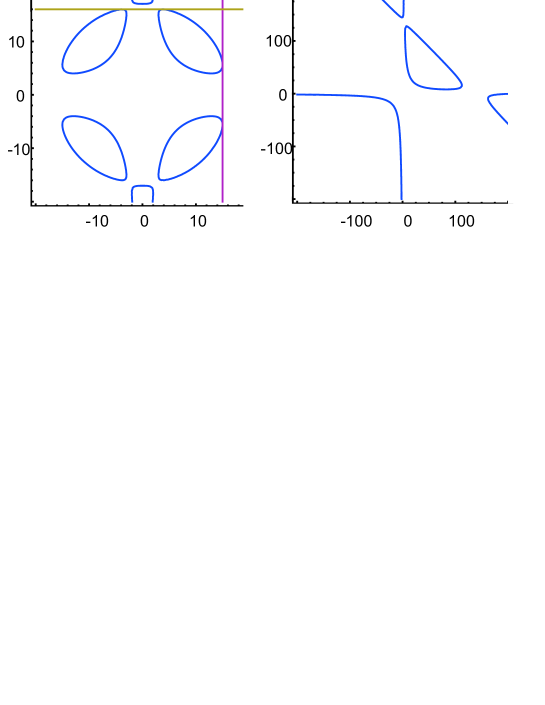
Figure 1. Diagonal relation in $x,y$ (left) and in $x^{2},y^{2}$ (right)

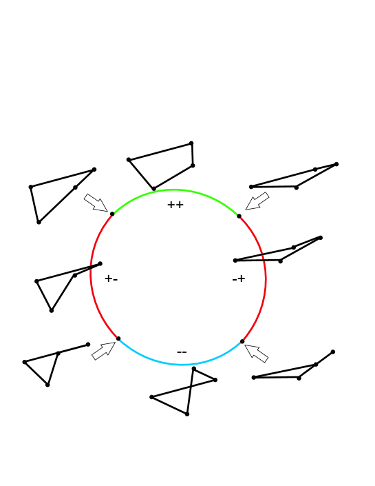
Figure 2. The configuration space $M(L)$ is divided into four parts

Consequently, the oval contains exactly 2 points where $\frac{\partial F}{\partial x}=0$ and two other points where $\frac{\partial F}{\partial y}=0$. These points divide the oval into 4 segments, each determined by the signs of partial derivatives (see Fig. 2).

1. Convex 4-gons (that is, $M^{C}$) correspond to the ”$++$” case. A vertex of configuration is aligned if the angle adjacent to it is $\pi$. For a non-degenerate 4-bar linkage, there exist exactly 2 vertices which can be aligned. The corresponding configurations are the boundary points of $M^{C}$.

2. Non-convex and non-self-intersecting 4-gons correspond to ”$+-$” and ”$-+$” parts.

3. Self-intersecting 4-gons correspond to the ”$--$” part.

We prove now that, for a convex $P$, we have $y^{\prime\prime}_{xx}<0$.

Indeed, locally $w$ is a function in $z$. We have $w=w(z)$, therefore $y^{2}=w(x^{2})$, which implies

$$y=w^{1/2}(x^{2})$$

$$y^{\prime}_{x}=w^{-1/2}xw_{z}^{\prime}.$$

We know from convexity of the elliptic curve that $w^{\prime\prime}_{zz}<0$.

$$y^{\prime\prime}_{xx}=\frac{w^{\prime}_{z}}{w^{2}}-\frac{x^{2}(w^{\prime}_{z})^{2}}{w^{3/2}}+\frac{2x^{2}w^{\prime\prime}_{zz}}{w^{1/2}}<0.$$

Assume that $P$ is a convex configuration which is critical for $E$.

$$E=\frac{t}{x}+\frac{1}{y}\ \ \hbox{ implies}$$

$$E^{\prime}_{x}=\frac{-t}{x^{2}}-\frac{y^{\prime}_{x}}{y^{2}},\ \hbox{ and}$$

$$E^{\prime\prime}_{xx}=\frac{2t}{x^{3}}+\frac{2[y^{\prime}(x)]^{2}}{y^{3}}-\frac{y^{\prime\prime}(x)}{y^{2}},\ \ \ \hbox{which is positive}.$$

Therefore, each critical point in the convex part is a local minimum.

So the statement (1) of the proposition is now straightforward: if there are two local minima, there should be a local maximum in between, which is impossible.

(2) For a non-intersecting 4-gon there is a flex strictly increasing both diagonals.

(3) There should be a maximum point of $E$ in $M(L)$. By what is proven above, the domain of self-intersecting 4-gons is the only possibility for it. ∎

Theorem 1.

1. We have a continuous bijection

   $$\varphi:(0,\infty)\rightarrow IntM^{C}(L)$$

   which maps a charge $t$ to the minimum point of $E$.

2. The mapping $\varphi$ extends to a bijection $\varphi:[0,\infty]\rightarrow M^{C}(L)$.

Proof. Point (1) follows from Proposition 1, (1) and Lemma 1. Point (2) follows from (1) and the above remark. ∎

Lemma 2.

Assume that $L$ is a 4-bar linkage, and the charge $t$ is zero. Then $E$ has exactly two critical points on $M(L)$: one minimum and one maximum.

Proof. The problem is reduced to finding the critical values of the diagonal $x$.∎

The lemma means that if we start at any configuration of any 4-gon $L$ and put zero charge at the ruling vertex, the gradient flow will bring us to the global minimum.

However, for other values of $t$, there might be extra local minima:

Example 1.

For $a=6,\ b=6.5,\ c=6.2,\ d=5.8$ and $t=2$, numerical computations show that there are four critical points of $E$ in total (see Fig. 3). The lengths of the diagonals and the values of $E$ (up to two decimals) are:

1. $x=0.50,\ y=3.24,\ E=2.61$ (local minimum)

2. $x=4.11,\ y=0.30,\ E=6.90$ (maximum)

3. $x=1.24,\ y=0.58,\ E=4.24$ (local maximum)

4. $x=9.59,\ y=7.60,\ E=0.36$ (minimum)

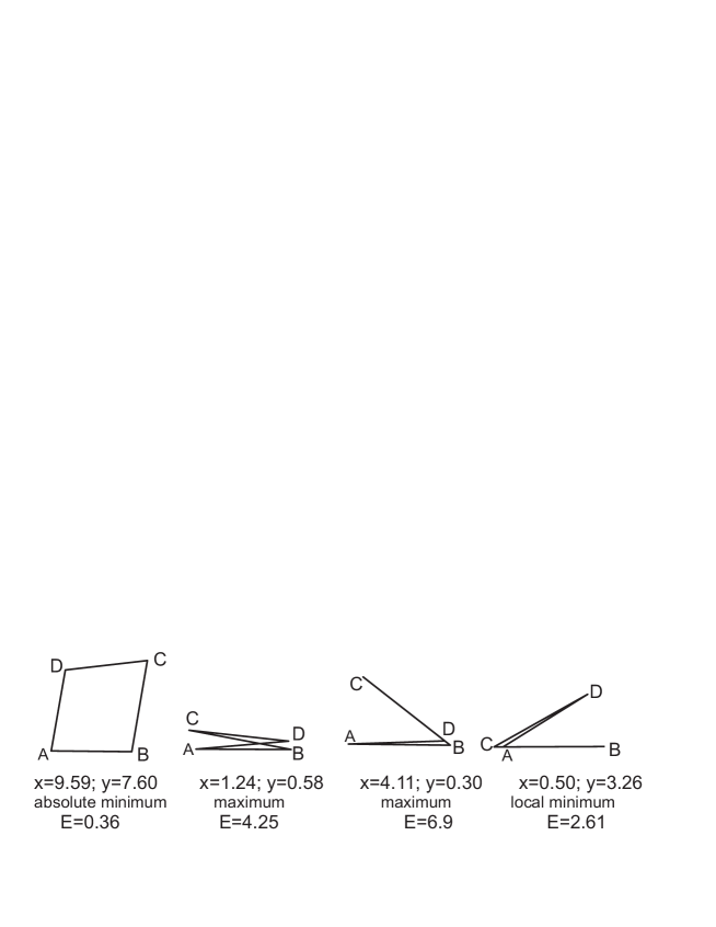
Figure 3. Critical configurations from Example 1

The above leads us to the following navigating algorithm.

Algorithm 1.

Assume we are given a 4-bar linkage $L$, its unknown starting configuration $P$ and a target convex configuration $P^{\prime}$. The following algorithm tells us how to reach $P^{\prime}$ by altering the ruling charge $t$.

1. Put the ruling charge $t=0$.

2. Compute the stabilizing charge $t^{\prime}$ of the configuration $P^{\prime}$.

3. Put the ruling charge $t=t^{\prime}$.

Remark 2.

If we allow non-positive charge and aim at non-convex configurations, the situation becomes more complicated. Example 1 shows that the number of (local) minima is greater than 1.

Remark 3.

If we put the same charged 4-bar linkage in 3D, we can skip step 1 in the above algorithm. Indeed, all critical points of $E$ are obviously planar configurations. Besides, unlike the 2D case, a local minimum cannot be self-intersecting: the unfolding flex increases both of the diagonals. Therefore, in 3D the potential $E$ has exactly one local minimum which is the global minimum.

Remark 4.

All above lemmata and Theorem 1 remain valid if we replace the Coulomb potential $E$ either by

$$E^{\alpha}=\sum\frac{q_{i}q_{j}}{(x_{ij})^{\alpha}},\ \ \alpha>0,$$ (4)

or by the limit version of (4)

$$E^{ln}=\sum q_{i}q_{j}\ln(x_{ij}).$$ (5)

3. Coulomb control of convex equilateral pentagons

Let $L$ be a equilateral $5$-bar linkage. In our setting we put two positive charges $s$ and $t$ at a pair of non-neighbouring vertices, say, at the third and fifth vertex of configuration. The charges of other vertices are constant and equal to $+1$. Then the (effective) Coulomb potential $E:M(L)\rightarrow\mathbb{R}$ is defined by the formula

$$E=\frac{1}{x_{14}}+\frac{1}{x_{24}}+\frac{t}{x_{13}}+\frac{s}{x_{25}}+\frac{st}{x_{35}},$$ (6)

where $x_{ij}$ are the lengths of diagonals of the configuration $V$.

We wish to understand whether two non-adjacent charges can provide a full control (in the same sense as for quadrilateral linkages) on convex configurations of $L$.

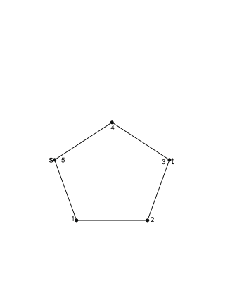
Figure 4.

Lemma 3.

Let $P\in\partial{M^{C}}$ be a critical point of $E$ for some charges $(s,t)$. Then $(s,t)$ never belongs to $(0,\infty)\times(0,\infty)$.

Proof. Assume the contrary: the charges $s$ and $t$ are both from $(0,\infty)$. A configuration is a boundary point of $M^{C}(L)$ whenever one of the vertices is aligned. Then by pulling the aligned vertex orthogonally to the adjacent edges (see Fig. 5) we get an infinitesimal flex which yields a first-order decrease of $E$.∎

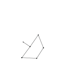
Figure 5.

Lemma 4.

For $s<0,\ t>0$, a convex pentagon is never a critical point of $E$.

Proof. Assume the contrary. Fix $x_{13}$ and compress $x_{25}$, see Figure 6. This yields an infinitesimal flex such that $E^{\prime}<0$. ∎

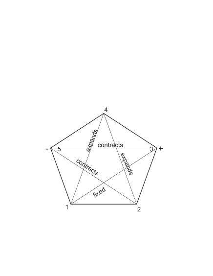
Figure 6.

Theorem 2.

For each strictly convex configuration $P$ of an equilateral pentagonal linkage, there exists exactly one $(s,t)\in(0,\infty)\times(0,\infty)$ such that $P$ is a critical point of $E$ for the charges $(s,t)$.

Proof. We start by reminding that

$$E=1/x_{14}+1/x_{24}+t/x_{13}+s/x_{25}+st/x_{35}.$$

Take the diagonals $x_{35}$ and $x_{13}$ as local coordinates in a neighborhood of $P$.

The polygon $P$ is a critical point of $E$ means that $dE$ vanishes:

$$-\partial E/\partial x_{35}=\alpha_{1}/x_{14}^{2}+\beta_{1}/x_{24}^{2}+s\gamma_{1}/x_{25}^{2}+\frac{st}{x_{35}^{2}}=0,$$

and

$$-\partial E/\partial x_{13}=\alpha_{2}/x_{14}^{2}+\beta_{2}/x_{24}^{2}+t/x_{13}^{2}+\frac{s\gamma_{2}}{x_{25}^{2}}=0,$$

where

$$\alpha_{1}=\partial x_{14}/\partial x_{35},\ \beta_{1}=\partial x_{24}/\partial x_{35},\ \ \gamma_{1}=\partial x_{25}/\partial x_{35},\hbox{ \ and}$$

$$\alpha_{2}=\partial x_{14}/\partial x_{13},\ \beta_{1}=\partial x_{24}/\partial x_{13},\ \ \gamma_{1}=\partial x_{25}/\partial x_{13}$$

We get a system in two variables $s$ and $t$ which reduces to the following quadratic equation in $s$:

$$A+Bs+Cs^{2}=0$$

with

$$A=\frac{\alpha_{1}}{x_{14}^{2}}+\frac{\beta_{1}}{x_{24}^{2}},$$

$$B=\frac{\gamma_{1}}{x_{25}^{2}}-\frac{x_{13}}{x_{35}^{2}}(\frac{\alpha_{2}}{x_{14}^{2}}+\frac{\beta_{2}}{x_{24}^{2}}),$$

$$\hbox{and \ \ \ }C=-\frac{x_{13}^{2}\gamma_{2}}{x_{35}^{2}x_{25}^{2}}.$$

It is sufficient to prove that $AC$ is negative. Then the equation has exactly one real positive solution $s$. By Lemma 4, $t$ is also positive.

Indeed, $AC$ is negative (and the proof is completed) because of the following sign analysis.

1. Consider the flex of $P$ which fixes $x_{13}$ and stretches $x_{35}$.

   $x_{14}$ compresses, therefore $\alpha_{1}=\partial x_{14}/\partial x_{35}<0$.

   $x_{24}$ compresses, therefore $\beta_{1}=\partial x_{24}/\partial x_{35}<0$.

   $x_{25}$ compresses, therefore $\gamma_{1}=\partial x_{25}/\partial x_{35}<0$.

2. Similarly, fixing $x_{35}$ and stretching $x_{13}$, we obtain that $\alpha_{2}<0$, $\beta_{2}<0$, and $\gamma_{2}<0$.

Let us give a more detailed explanation why the above inequalities hold. As an example, let us prove that if the diagonal $x_{13}$ is fixed, and the diagonal $x_{35}$ gets longer, then $x_{24}$ compresses (see Fig. 7).

We can assume that the three points 1,2,3 are fixed and that the points 4 and 5 are moving with infinitesimal velocities $v_{4}$ and $v_{5}$. The vector $v_{4}$ is orthogonal to the edge $43$. By convexity, the angle between $v_{4}$ and the diagonal $24$ is smaller than $\pi/2$, which implies the claim. ∎

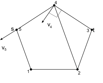
Figure 7.

Remark 5.

If we try to rule by putting charges at adjacent vertices (say, at the vertices 1 and 2), the situation gets worse: we reach not all of the convex polygons. For instance, we will never be able to have simultaneously the vertices 5 and 3 aligned. By continuity, an entire neighborhood of such a polygon becomes unreachable.

4. Concluding remarks

Our results suggest several natural problems and conjectures concerned with the Coulomb control scenario for $n$-bar linkages with arbitrary $n$. In particular, there is good evidence that, for equilateral linkages, the complete Coulomb control of convex configurations is valid if we are permitted to choose controlling charges at ALL vertices.

Assuming that this conjecture is true, what is the minimal number of controlling charges sufficient to provide complete Coulomb control? For dimension reasons, one may await that it should be sufficient to have $n-3$ controlling charges. Is this amount of controlling charges indeed sufficient for any $n$-bar linkage?

Several interesting problems in the spirit of the famous Maxwell conjecture [8] are concerned with estimating the amount and possible types of critical points of Coulomb potential in the moduli space of linkage. In particular, what is the exact upper bound for the number of critical points of Coulomb potential in the planar moduli space of generic $n$-bar linkage? We conjecture that, for a generic $4$-bar linkage, the Coulomb potential can have not more than four critical points and their types are the same as in Example 1.

Analogous problems are also meaningful and interesting for all potentials of the form (4), (5). These and further aspects of the Coulomb control scenario will be addressed in forthcoming publications of the authors.

References

- [1] R.Connelly, E.Demaine, Geometry and topology of plygonal linkages, Handbook of discrete and computational geometry, 2nd ed. CRC Press, Boca Raton, 2004, 197-218.
- [2] M. Farber, Invitation to Topological Robotics, Zuerich Lectures in Advanced Mathematics. European Mathematical Society (EMS), Zuerich, 2008.
- [3] A.Gabrielov, D.Novikov, B.Shapiro, Mystery of point charges, Proc. Lond. Math. Soc. 95, 2007, 443-472.
- [4] G. Khimshiashvili, G. Panina, Cyclic polygons are critical points of area. Zap. Nauchn. Sem. S.-Peterburg. Otdel. Mat. Inst. Steklov. (POMI), 2008, 360, 8, 238–245.
- [5] G.Khimshiashvili, D.Siersma, Cyclic configurations of planar multiple penduli, ICTP Preprint IC/2009/047. 11 p.
- [6] G. Khimshiashvili, G. Panina, D. Siersma, A. Zhukova, Critical configurations of planar robot arms, Centr. Europ. J. Math., 2013, 11, 3, 519–529.
- [7] T. Kudernac,N. Ruangsupapichat, M. Parschau, B. Mac, N. Katsonis, S. Harutyunyan, K.-H. Ernst, B. Feringa, (2011). Electrically driven directional motion of a four-wheeled molecule on a metal surface”. Nature 479 (7372): 208–11.
- [8] J.C.Maxwell, A Treatise on Electricity and Magnetism, London, 1853.
- [9] G. Panina, Moduli space of a planar polygonal linkage: a combinatorial description. arXiv:1209.3241