Stoneley waves and interface stability
of Bell materials in compression;
Comparison with rubber.

Abstract

Two semi-infinite bodies made of prestressed, homogeneous, Bell-constrained, hyperelastic materials are perfectly bonded along a plane interface. The half-spaces have been subjected to finite pure homogeneous predeformations, with distinct stretch ratios but common principal axes, and such that the interface is a common principal plane of strain. Constant loads are applied at infinity to maintain the deformations and the influence of these loads on the propagation of small-amplitude interface (Stoneley) waves is examined. In particular, the secular equation is found and necessary and sufficient conditions to be satisfied by the stretch ratios to ensure the existence of such waves are given. As the loads vary, the Stoneley wave speed varies accordingly: the upper bound is the ‘limiting speed’ (given explicitly), beyond which the wave amplitude cannot decay away from the interface; the lower bound is zero, where the interface might become unstable. The treatment parallels the one followed for the incompressible case and the differences due to the Bell constraint are highlighted. Finally, the analysis is specialized to specific strain energy densities and to the case where the bimaterial is uniformly deformed (that is when the stretch ratios for the upper half-space are equal to those for the lower half-space.) Numerical results are given for ‘simple hyperelastic Bell’ materials and for ‘Bell’s empirical model’ materials, and compared to the results for neo-Hookean incompressible materials.

1 INTRODUCTION

This paper is a prolongation of a series of articles concerned with the propagation of small-amplitude waves in deformed Bell materials. Beatty and Hayes [1] wrote the incremental equations of motion for a hyperelastic body maintained in a state of static finite homogeneous deformation and subject to the constraint of Bell [2]: tr $\mathbf{V}=3$, where $\mathbf{V}$ is the left stretch tensor associated with the finite deformation. They studied plane [1] as well as torsional [3] waves. Then this author [4] found the secular equation for surface (Rayleigh) waves propagating on a semi-infinite deformed body made of Bell-constrained material. Next [5] the surface stability of such a half-space under compression was analyzed and compared with that of incompressible rubber. Now the propagation of interface (Stoneley) waves is considered for two rigidly bonded semi-infinite bodies made of distinct Bell materials. Each half-space was subjected to a finite homogeneous predeformation and the principal axes of each deformation are assumed to coincide at the interface, which is a common principal plane. Moreover, the interfacial wave is assumed to propagate in a principal direction. These common [6, 7] restrictions aside, a general necessary and sufficient condition of existence of a Stoneley wave is established, together with the corresponding secular equation.

These general results are obtained in Section 3, after the basic equations of the problem have been written in Section 2. For purposes of comparison and contrast, these latter equations are written in a manner which is similar to those governing the propagation of interfacial waves in deformed hyperelastic materials subject to the constraint of incompressibility, det $\mathbf{V}=1$. Then in Section 4, the analysis is specialized to the case where the infinite body made of the two bonded half-spaces is uniformly prestrained, that is when the principal stretch ratios of strain are the same for the upper half-space and for the lower half-space. For “simple hyperelastic Bell” materials, the influence of the initial deformation on the wave speed is highlighted. As the half-spaces are more and more compressed, this speed tends to zero and the secular equation gives the “neutral equation”. The critical stretch ratios, at which the neutral equation is reached, are obtained. In the case of a plane prestrain, these critical stretches, and the corresponding ones for “Bell’s empirical model”, are compared with the critical stretches obtained by Biot [8] for the interfacial stability of (incompressible) neo-Hookean materials, often used to model rubber. The conclusion is that, as far as interfacial stability is concerned, rubber may be compressed more than Bell’s empirical materials, but not as much as Bell simple hyperelastic materials, before the critical stretches are reached.

2 PRELIMINARIES

2.1 Deformed Bell half-spaces

Consider two semi-infinite bodies made of different homogeneous Bell-constrained hyperelastic materials, separated by plane interface $x_{2}=0$. Initially, each body is at rest in a reference configuration, denoted by $\mathcal{B}_{0}$ for the lower half-space $x_{2}\geq 0$, and by $\mathcal{B}^{*}_{0}$ for the upper half-space $x_{2}\leq 0$. The constitutive equation for the lower half-space is [2]

$$\mathbf{T}=p\mathbf{V}+\omega_{0}\mathbf{1}+\omega_{2}\mathbf{V}^{2},$$ (1)

expressing the Cauchy stress tensor $\mathbf{T}$ in terms of the left stretch tensor $\mathbf{V}$. Here $p$ is an undetermined scalar, to be found from the equations of motion or of equilibrium, and from the boundary conditions. The constitutive parameters $\omega_{0}$ and $\omega_{2}$ are defined in terms of the derivatives of the strain energy density $\Sigma=\Sigma(i_{2},i_{3})$ of the hyperelastic body with respect to the principal invariants $i_{2}=[(\text{tr }\mathbf{V})^{2}-\text{tr }(\mathbf{V}^{2})]/2$, $i_{3}=\text{det }\mathbf{V}$, as

$$\omega_{0}=\partial\Sigma/\partial i_{3}\leq 0,\quad\omega_{2}=-i_{3}^{-1}\partial\Sigma/\partial i_{2}>0.$$ (2)

The inequalities above are called the ‘Beatty-Hayes $A$-inequalities’ [2]. Also, the Bell constraint is satisfied at all times:

$$i_{1}\equiv\text{tr }\mathbf{V}=3.$$ (3)

Similar (starred) equalities and inequalities apply for the upper half-space $x_{2}\leq 0$.

Next, consider that each half-space is subject to a finite static pure homogeneous static deformation $\mathcal{B}_{0}\rightarrow\mathcal{B}_{1}$ and $\mathcal{B}^{*}_{0}\rightarrow\mathcal{B}^{*}_{1}$ by the application of suitable loads. The principal axes of these deformations along $x_{2}$, and $x_{1}$ and $x_{3}$, two orthogonal directions in the $x_{2}=0$ plane. Hence the finite deformations are described in the coordinate system of the principal axes by

$$x_{\Gamma}=\lambda_{\Gamma}X_{\Gamma}\quad(x_{2}\geq 0),\quad\text{and}\quad x_{\Gamma}=\lambda^{*}_{\Gamma}X_{\Gamma}\quad(x_{2}\leq 0),\quad(\Gamma=1,2,3;\text{no sum}),$$ (4)

where the $\lambda_{\Gamma}$, $\lambda^{*}_{\Gamma}$ are the principal stretch ratios for each half-space. For the lower half-space we have

$$\mathbf{V}=\text{Diag}(\lambda_{1},\lambda_{2},\lambda_{3}),$$

$$\lambda_{1}+\lambda_{2}+\lambda_{3}=3,\quad i_{2}=\lambda_{1}\lambda_{2}+\lambda_{2}\lambda_{3}+\lambda_{3}\lambda_{1},\quad i_{3}=\lambda_{1}\lambda_{2}\lambda_{3},$$ (5)

and the following constant Cauchy stress tensor

$$T_{\Gamma\Gamma}=p_{o}\lambda_{\Gamma}+\omega_{0}+\omega_{2}\lambda_{\Gamma}^{2}\quad(\Gamma=1,2,3;\text{no sum}),\quad T_{ij}=0\quad(i\neq j),$$ (6)

where $p_{o}$ is constant, and $\omega_{0}$, $\omega_{2}$ are given by (2) and valuated at $i_{2}$, $i_{3}$ given by (2.1)_3,4, clearly satisfies the equilibrium equations $T_{ij,j}=0$. So does $\mathbf{T}^{*}$, the equivalent starred version for the upper half-space. Finally, the half-spaces are rigidly bounded. At the interface $x_{2}=0$, the continuity of the tractions imposes that

$$p_{o}\lambda_{2}+\omega_{0}+\lambda_{2}^{2}\omega_{2}=p_{o}^{*}\lambda^{*}_{2}+\omega^{*}_{0}+\lambda^{*2}_{2}\omega^{*}_{2}.$$ (7)

The half-spaces are maintained in these deformed states $\mathcal{B}_{1}$, $\mathcal{B}^{*}_{1}$ by the application at infinity of the loads $P_{\Gamma}=-T_{\Gamma\Gamma}$, $P^{*}_{\Gamma}=-T^{*}_{\Gamma\Gamma}$. It follows from (7) that $P_{2}=P^{*}_{2}$.

2.2 Small-amplitude interface wave

Now consider that a small amplitude wave travels with speed $v$ and a wave number $k$ at the interface, in the direction of $x_{1}$, with attenuation away from $x_{2}=0$. The following expressions describe this incremental motion $\mathcal{B}_{1}\rightarrow\overline{\mathcal{B}}_{1}$, $\mathcal{B}^{*}_{1}\rightarrow\overline{\mathcal{B}}^{*}_{1}$:

$$\overline{\mathbf{x}}=\mathbf{x}+\varepsilon\Re\{\mathbf{U}(kx_{2})e^{ik(x_{1}-vt)}\},\quad\text{and}\quad\overline{\mathbf{x}}=\mathbf{x}+\varepsilon\Re\{\mathbf{U}^{*}(kx_{2})e^{ik(x_{1}-vt)}\},$$ (8)

for $x_{2}\geq 0$ and for $x_{2}\leq 0$, respectively. Here $\varepsilon$ is small enough to allow linearization and the amplitudes $\mathbf{U}$ and $\mathbf{U}^{*}$ are of the form $\mathbf{U}=[U_{1},U_{2},0]^{\mathrm{T}}$, $\mathbf{U}^{*}=[U^{*}_{1},U^{*}_{2},0]^{\mathrm{T}}$. The remainder of this paper is devoted to the study of these interfacial (Stoneley) waves. Dowaikh and Ogden [6] and Chadwick [7] conducted similar studies for prestrained incompressible and compressible materials, respectively. In both cases, the authors proved that the initial normal traction $T_{22}=T^{*}_{22}$ played no role in the resolution and analysis of the problem. It can be checked that such is also the case for deformed Bell materials and without loss of generality, we choose $T_{22}=T^{*}_{22}=0$, and thus $P_{2}=P_{2}^{*}=0$ (of course, the traction $T_{22}$ might play a role in issues other than the derivation of the secular equation for Stoneley waves.) Hence the following loads $P_{1}=-T_{11}$, $P_{3}=-T_{33}$ and $P^{*}_{1}$, $P^{*}_{3}$ are applied at $x_{1}=\pm\infty$ and $x_{3}=\pm\infty$ in order to sustain the finite homogeneous deformation,

$$P_{\Gamma}=(\lambda_{2}-\lambda_{\Gamma})(-\omega_{0}+\lambda_{\Gamma}\lambda_{2}\omega_{2})/\lambda_{2},$$

$$P^{*}_{\Gamma}=(\lambda^{*}_{2}-\lambda^{*}_{\Gamma})(-\omega^{*}_{0}+\lambda^{*}_{\Gamma}\lambda^{*}_{2}\omega^{*}_{2})/\lambda^{*}_{2},$$

$$(\Gamma=1,3).$$ (9)

Moreover, this assumption enables us to use previously established results for the incremental equations of motion. Specifically, the equations are written as the following system of first order differential equations for the components of the displacements $\mathbf{U}$, $\mathbf{U}^{*}$, and of the tractions $\mathbf{t}$, $\mathbf{t}^{*}$ on the planes $x_{2}=$ const. (see Ref.[4] for details):

$$b_{3}\lambda_{2}^{2}U_{1}^{\prime}+ib_{3}\lambda_{2}^{2}U_{2}-t_{1}=0, t_{1}^{\prime}+i\lambda_{1}\lambda_{2}^{-1}t_{2}-(\lambda_{1}\lambda_{2}^{-1}C-\rho v^{2})U_{1}=0,$$

$$U_{2}^{\prime}+i\lambda_{1}\lambda_{2}^{-1}U_{1}=0, t_{2}^{\prime}+it_{1}-[b_{3}(\lambda_{1}^{2}-\lambda_{2}^{2})-\rho v^{2}]U_{2}=0,$$ (10)

where

$$b_{3}=\frac{-\omega_{0}+\lambda_{1}\lambda_{2}\omega_{2}}{\lambda_{2}(\lambda_{1}+\lambda_{2})},$$

$$C=\lambda_{1}^{-1}\lambda_{2}C_{11}+\lambda_{1}\lambda_{2}^{-1}C_{22}-C_{12}-C_{21}-2\omega_{0}-(\lambda_{1}^{2}+\lambda_{2}^{2})\omega_{2},$$

$$C_{ij}=2\lambda^{2}_{i}\delta_{ij}\omega_{2}-\lambda_{j}^{2}(\omega_{02}+\lambda_{i}^{2}\omega_{22})+\lambda_{1}\lambda_{2}\lambda_{3}(\omega_{03}+\lambda_{i}^{2}\omega_{23}),$$ (11)

for $x_{2}\geq 0$, and a starred version for $x_{2}\leq 0$. Here $\rho$ ($\rho^{*}$) is the mass density of the lower (upper) half-space, and the derivatives $\omega_{0\Gamma}$, $\omega_{2\Gamma}$ ($\Gamma=2,3$) of the material parameters $\omega_{0}$, $\omega_{2}$ are taken with respect to $i_{\Gamma}$ and evaluated at $i_{2}$, $i_{3}$ given by (2.1). The half-spaces are rigidly bonded at $x_{2}=0$ so that the following boundary conditions apply,

$$\mathbf{U}(0)=\mathbf{U}^{*}(0),\quad\mathbf{t}(0)=\mathbf{t}^{*}(0),$$ (12)

together with the requirement that the wave vanishes as $x_{2}\rightarrow\pm\infty$.

3 GENERAL PREDEFORMATIONS AND STRAIN ENERGY FUNCTIONS

Here we solve the problem at hand, that is we solve the equations of motion (2.2) and then apply the boundary conditions (12) in order to derive the secular equation for the speed of Stoneley waves in deformed Bell materials. We adopt an approach reminiscent of that used by Dowaikh and Ogden [6] for Stoneley waves in incompressible materials and show how each constraint leads to different results.

3.1 Secular equation; comparison with incompressible materials

For small-amplitude waves of the form (8)₁, the incremental constraint of incompressibility, $u_{1,1}+u_{2,2}+u_{3,3}=0$, imposes that

$$iU_{1}+U^{\prime}_{2}=0,$$ (13)

suggesting the introduction of the function $\hat{\varphi}$ defined by

$$U_{1}(kx_{2})=i\hat{\varphi}^{\prime}(kx_{2}),\quad U_{2}(kx_{2})=\hat{\varphi}(kx_{2}).$$ (14)

In our context, the incremental constraint of Bell, $\lambda_{1}u_{1,1}+\lambda_{2}u_{2,2}+\lambda_{3}u_{3,3}=0$, imposes Eq.(2.2)₃, that is

$$i\lambda_{1}\lambda_{2}^{-1}U_{1}+U^{\prime}_{2}=0,$$

suggesting the function $\varphi$ defined by

$$U_{1}(kx_{2})=i\varphi^{\prime}(k\lambda_{1}\lambda_{2}^{-1}x_{2}),\quad U_{2}(kx_{2})=\varphi(k\lambda_{1}\lambda_{2}^{-1}x_{2}).$$ (15)

From (2.2)_4,1, the traction components are also expressed in terms of $\varphi$ and its derivatives:

$$t_{1}=ib_{3}\lambda_{2}^{2}(\lambda_{1}\lambda_{2}^{-1}\varphi^{\prime\prime}+\varphi),\quad t_{2}=-b_{3}\lambda_{1}\lambda_{2}\varphi^{\prime\prime\prime}+\lambda_{1}^{-1}\lambda_{2}(\lambda_{1}\lambda_{2}^{-1}C-b_{3}\lambda_{1}\lambda_{2}-\rho v^{2})\varphi^{\prime}.$$ (16)

Finally, Eq.(2.2)₂ reads

$$b_{3}\lambda_{1}^{2}\varphi^{\prime\prime\prime\prime}-(\lambda_{1}\lambda_{2}^{-1}C-2b_{3}\lambda_{1}\lambda_{2}-\rho v^{2})\varphi^{\prime\prime}+(b_{3}\lambda_{1}^{2}-\rho v^{2})\varphi=0.$$ (17)

The same procedure is of course also valid for the upper half-space, with the introduction of a function $\varphi^{*}$.

Dowaikh and Ogden [6] expressed the strain energy density as a function $\hat{W}(\lambda_{1},\lambda_{2},\lambda_{3})$ of the principal stretches of deformation, rather than as a function of the invariants $\hat{\Sigma}(i_{1},i_{2},i_{3})$, a practice also favored by Biot [9]. With this choice, and the introduction of the function $\hat{\varphi}$ in (15), they proved that for incompressible materials, the counterpart to (17) is

$$\hat{\gamma}\hat{\varphi}^{\prime\prime\prime\prime}-(2\hat{\beta}-\rho v^{2})\hat{\varphi}^{\prime\prime}+(\hat{\alpha}-\rho v^{2})\hat{\varphi}=0,$$ (18)

where $\hat{\alpha}$, $\hat{\beta}$, and $\hat{\gamma}$ are defined in terms of $\hat{W}$ and its derivatives with respect to the $\lambda_{i}$ as

$$\hat{\alpha}\lambda_{2}^{2}=\hat{\gamma}\lambda_{1}^{2}=(\lambda_{1}\hat{W}_{1}-\lambda_{2}\hat{W}_{2})\lambda_{1}^{2}\lambda_{2}^{2}/(\lambda_{1}^{2}-\lambda_{2}^{2}),$$

$$2\hat{\beta}+2\hat{\gamma}=\lambda_{1}^{2}\hat{W}_{11}+\lambda_{2}^{2}\hat{W}_{22}-2\lambda_{1}\lambda_{2}\hat{W}_{12}+2\lambda_{2}\hat{W}_{2}.$$ (19)

Also, for incompressible materials, the assumption of strong ellipticity for the equations of motion implies that

$$\hat{\alpha}>0,\quad\hat{\gamma}>0,\quad\hat{\beta}+\sqrt{\hat{\alpha}\hat{\gamma}}>0.$$ (20)

For Bell constrained materials, introduce by analogy $\alpha$, $\beta$, and $\gamma$, defined by

$$\alpha=b_{3}\lambda_{1}^{2},\quad\gamma=b_{3}\lambda_{2}^{2},\quad 2\beta+2\sqrt{\alpha\gamma}=\lambda_{1}\lambda_{2}^{-1}C,$$ (21)

or equivalently, by

$$\alpha\lambda_{2}^{2}=\gamma\lambda_{1}^{2}=(W_{1}-W_{2})\lambda_{1}^{2}\lambda_{2}/[\lambda_{3}(\lambda_{1}^{2}-\lambda_{2}^{2})],$$

$$2\beta+2\sqrt{\alpha\gamma}=(W_{11}+W_{22}-2W_{12})\lambda_{1}/(\lambda_{2}\lambda_{3}).$$ (22)

Now rewrite the equation of motion (17) as

$$\alpha\varphi^{\prime\prime\prime\prime}-(2\beta-\rho v^{2})\varphi^{\prime\prime}+(\alpha-\rho v^{2})\varphi=0.$$ (23)

Using the strong ellipticity condition for the equations of motion in deformed Bell materials (see Appendix) together with Eqs.(2) and (2.2), we also find the following inequalities,

$$\alpha>0,\quad\gamma>0,\quad\beta+\alpha>0.$$ (24)

The contrast between the effects of incompressibility and of the Bell constraint is striking (compare for instance the first term in (18) and in (23).) Now Equation (23) and its starred version for the upper half-space are solved.

Because Stoneley waves vanish with distance from the interface, the solutions $\varphi$ and $\varphi^{*}$ must be of the form

$$\varphi(z)=Ae^{-s_{1}z}+Be^{-s_{2}z}\quad(z\geq 0),\quad\varphi^{*}(z)=A^{*}e^{s_{1}^{*}z}+B^{*}e^{s_{2}^{*}z}\quad(z\leq 0),$$ (25)

where $s_{1}\neq s_{2}$, $\Re(s_{i})>0$, $s^{*}_{1}\neq s^{*}_{2}$, $\Re(s^{*}_{i})>0$, for some constants $A$, $B$, $A^{*}$, $B^{*}$. Explicitly, the $s_{i}$, $s^{*}_{i}$ are roots of the biquadratics

$$\alpha s^{4}-(2\beta-\rho v^{2})s^{2}+\alpha-\rho v^{2}=0, \alpha^{*}s^{*4}-(2\beta^{*}-\rho^{*}v^{2})s^{*2}+\alpha^{*}-\rho^{*}v^{2}=0,$$

$$s_{1}^{2}+s_{2}^{2}=(2\beta-\rho v^{2})/\alpha, s_{1}^{*2}+s_{2}^{*2}=(2\beta^{*}-\rho^{*}v^{2})/\alpha^{*},$$

$$s_{1}^{2}s_{2}^{2}=(\alpha-\rho v^{2})/\alpha, s_{1}^{*2}s_{2}^{*2}=(\alpha^{*}-\rho^{*}v^{2})/\alpha^{*}.$$ (26)

The roots $s_{1}^{2}$ and $s_{2}^{2}$ of the real quadratic (3.1)₁ are either both real or both complex; if they are real, they are non-negative, otherwise $s_{1}$ and $s_{2}$ are purely imaginary in contradiction with the decaying requirement $\Re(s_{i})>0$; if they are complex, they are conjugate, because the coefficients of (3.1)₁ are real. In both cases, $s_{1}^{2}s_{2}^{2}\geq 0$ and similarly, $s_{1}^{*2}s_{2}^{*2}\geq 0$, so that

$$0\leq v\leq\text{min}\{v_{L},v^{*}_{L}\},\quad\text{where}\quad v_{L}=\sqrt{\alpha/\rho},\;v^{*}_{L}=\sqrt{\alpha^{*}/\rho^{*}}.$$ (27)

In fact, the interval of possible values for $v$ for which the wave decays away from the interface (the subsonic interval) might be smaller than the interval defined above. This point is clarified in §3.2. For the time being, we derive an explicit expression for the secular equation. Equations (12) express the continuity of the displacement and traction incremental amplitudes at the interface $x_{2}=0$. Using the expressions (14), (16) of $U_{i}$, $U_{i}^{*}$, $t_{i}$, $t^{*}_{i}$, in terms of $\varphi$, $\varphi^{*}$ and their derivatives, they lead to

$$\varphi(0)=\varphi^{*}(0),\quad\varphi^{\prime}(0)=\varphi^{*^{\prime}}(0),$$

$$\gamma[\sqrt{\frac{\gamma}{\alpha}}\varphi^{\prime\prime}(0)+\varphi(0)]=\gamma^{*}[\sqrt{\frac{\gamma^{*}}{\alpha^{*}}}\varphi^{*^{\prime\prime}}(0)+\varphi^{*}(0)],$$ (28)

$$-\sqrt{\alpha\gamma}\varphi^{\prime\prime\prime}(0)+\sqrt{\frac{\gamma}{\alpha}}(2\beta+\sqrt{\alpha\gamma}-\rho v^{2})\varphi^{\prime}(0)=$$

$$\phantom{-\sqrt{\alpha\gamma}\varphi^{\prime\prime\prime}(0)+\sqrt{\frac{\gamma}{\alpha}}}-\sqrt{\alpha^{*}\gamma^{*}}\varphi^{*^{\prime\prime\prime}}(0)+\sqrt{\frac{\gamma^{*}}{\alpha^{*}}}(2\beta^{*}+\sqrt{\alpha^{*}\gamma^{*}}-\rho v^{2})\varphi^{*^{\prime}}(0).$$

Using (3.1)_3,4 and (25), we rewrite this system as four homogeneous linear equations for the unknowns $A$, $B$, $A^{*}$, $B^{*}$:

$$A+B=A^{*}+B^{*},$$

$$s_{1}A+s_{2}B=-s^{*}_{1}A^{*}-s^{*}_{2}B^{*},$$

$$(\sqrt{\alpha\gamma}s_{1}^{2}+\gamma)A+(\sqrt{\alpha\gamma}s_{2}^{2}+\gamma)B=$$

$$\quad\quad\quad\quad(\sqrt{\alpha^{*}\gamma^{*}}s_{1}^{*2}+\gamma^{*})A^{*}+(\sqrt{\alpha^{*}\gamma^{*}}s_{2}^{*2}+\gamma^{*})B^{*},$$

$$s_{1}(\sqrt{\alpha\gamma}s_{2}^{2}+\gamma)A+s_{2}(\sqrt{\alpha\gamma}s_{1}^{2}+\gamma)B=$$

$$\quad\quad\quad\quad-s^{*}_{1}(\sqrt{\alpha^{*}\gamma^{*}}s_{2}^{*2}+\gamma^{*})A^{*}-s^{*}_{2}(\sqrt{\alpha^{*}\gamma^{*}}s_{1}^{*2}+\gamma^{*})B^{*}.$$ (29)

The vanishing of the corresponding determinant yields the secular equation. Dropping the factor $(s_{1}-s_{2})(s^{*}_{1}-s^{*}_{2})$ and using the quantities $\eta$, $r$ (and $\eta^{*}$, $r^{*}$) defined as follows,

$$\eta=\sqrt{\frac{\alpha-\rho v^{2}}{\alpha}},\quad r=\sqrt{(\eta+1)^{2}+2\frac{\beta-\alpha}{\alpha}},$$ (30)

the secular equation is written compactly as

$$i(v) \equiv\gamma^{2}[\frac{\alpha}{\gamma}\eta r^{2}-(\sqrt{\frac{\alpha}{\gamma}}\eta-1)^{2}]+\gamma^{*2}[\frac{\alpha^{*}}{\gamma^{*}}\eta^{*}r^{*2}-(\sqrt{\frac{\alpha^{*}}{\gamma^{*}}}\eta^{*}-1)^{2}]$$

$$\quad+\gamma\gamma^{*}[\sqrt{\frac{\alpha\alpha^{*}}{\gamma\gamma^{*}}}(\eta+\eta^{*})rr^{*}+2(\sqrt{\frac{\alpha}{\gamma}}\eta-1)(\sqrt{\frac{\alpha^{*}}{\gamma^{*}}}\eta^{*}-1)]$$ (31)

$$=0.$$

The quantities $\eta$, $\eta^{*}$ are real by (27) and so are $r$, $r^{*}$, at least as long as the decaying condition is satisfied. We now elaborate on this last point.

3.2 The subsonic interval

From (3.1) and the definition (30) of $r$, expressions for the squared sum and difference of the roots $s_{i}$ follow:

$$(s_{1}+s_{2})^{2}=r^{2},\quad(s_{1}-s_{2})^{2}=s^{2},$$ (32)

where

$$s^{2}=\frac{2\beta-\rho v^{2}}{\alpha}-2\sqrt{\frac{\alpha-\rho v^{2}}{\alpha}}=(\eta-1)^{2}+2\frac{\beta-\alpha}{\alpha}=r^{2}-4\eta.$$ (33)

Hence the requirement of exponential decay $\Re(s_{i})>0$ is equivalent to

$$\Re(r\pm s)>0.$$ (34)

Now we span the subsonic range, that is the interval $I$ (say) of possible values for $v$ such that (34) is satisfied. This interval is $I=[0,\hat{v}]$ where $\hat{v}$ is called the limiting speed.

Starting at $v=0$, we have, using the strong ellipticity condition (24)₃,

$$v=0,\quad\eta=1,\quad r=\sqrt{2\frac{\beta+\alpha}{\alpha}}>0,\quad r^{2}-s^{2}=4>0,$$ (35)

so that (34) is satisfied.

Now, if $2\beta-\alpha>0$, then we may increase $v$ from $0$ to $v_{L}=\sqrt{\alpha/\rho}$, where

$$v=v_{L},\quad\eta=0,\quad r=\sqrt{\frac{2\beta-\alpha}{\alpha}}>0,\quad r^{2}-s^{2}=0,$$ (36)

and $\eta$, $r$, $r^{2}-s^{2}$, decrease monotonically with $v$ but remain non-negative real numbers, so that (34) is satisfied over the interval $[0,v_{L}]$. Clearly in this situation, the limiting speed is $\hat{v}=v_{L}=\sqrt{\alpha/\rho}$.

However, in the situation where $2\beta-\alpha<0$, we may increase $v$ from $0$ only up to $\tilde{v}$ (where $r=0$) in order to satisfy (34), where $\tilde{v}$ is defined by

$$\rho\tilde{v}^{2}=2[\beta-\alpha+\sqrt{2\alpha(\alpha-\beta)}]<\alpha=\rho v_{L}^{2}.$$ (37)

Clearly the limiting speed is then $\hat{v}=\tilde{v}$.

Conducting a similar analysis for the upper half-space, we conclude that the limiting speed is

$$\hat{v}=\left\{\begin{array}[]{lll}&\text{min}\{v_{L},v^{*}_{L}\},&\text{when}\quad 2\beta>\alpha,2\beta^{*}>\alpha^{*},\\ &\text{min}\{\tilde{v},v^{*}_{L}\},&\text{when}\quad 2\beta<\alpha,2\beta^{*}>\alpha^{*},\\ &\text{min}\{v_{L},\tilde{v}^{*}\},&\text{when}\quad 2\beta>\alpha,2\beta^{*}<\alpha^{*},\\ &\text{min}\{\tilde{v},\tilde{v}^{*}\},&\text{when}\quad 2\beta<\alpha,2\beta^{*}<\alpha^{*}.\end{array}\right.$$ (38)

Note that the analysis conducted in this subsection (defining the subsonic interval) and in the following one (defining the conditions of existence of a Stoneley wave) rely directly upon the methods developed by Chadwick [7] for compressible materials, with the modifications required to accommodate the Bell constraint.

3.3 Existence and uniqueness of interfacial (Stoneley) waves; comparison with surface (Rayleigh) waves

Here we derive the conditions of existence for a Stoneley wave at the interface of two deformed Bell-constrained half-spaces, using a “matrix reformulation” of the secular equation (3.1), a method suggested by Chadwick [7] and based on the surface impedance method of Barnett et al. [10]. Indeed, introducing the following symmetric $2\times 2$ matrices

$$\mathbf{M}(v)=\gamma\begin{bmatrix}\sqrt{\frac{\alpha}{\gamma}}\eta r&1-\sqrt{\frac{\alpha}{\gamma}}\eta\\ 1-\sqrt{\frac{\alpha}{\gamma}}\eta&\sqrt{\frac{\alpha}{\gamma}}r\end{bmatrix},\quad\mathbf{M}^{*}(v)=\gamma^{*}\begin{bmatrix}\sqrt{\frac{\alpha^{*}}{\gamma^{*}}}\eta^{*}r^{*}&\sqrt{\frac{\alpha^{*}}{\gamma^{*}}}\eta^{*}-1\\ \sqrt{\frac{\alpha^{*}}{\gamma^{*}}}\eta^{*}-1&\sqrt{\frac{\alpha^{*}}{\gamma^{*}}}r^{*}\end{bmatrix},$$ (39)

we find that the secular equation (3.1) corresponds to

$$i(v)=\text{det }\mathbf{N}(v)=0,\quad\text{where}\quad\mathbf{N}(v)=\mathbf{M}(v)+\mathbf{M}^{*}(v).$$ (40)

From then on, it is an easy matter to transpose Chadwick’s results [7] for incompressible materials to Bell materials, and to show inter alia that the eigenvalues of $\mathbf{N}(v)$ decrease monotonically as $v$ increases in $I$. Then the following results apply (see also Barnett et al. [10] for Stoneley waves in linear anisotropic elasticity): when an interfacial wave exists, it is unique; it propagates at a speed which is greater than the speed of the Raleigh wave associated with either each half-space; it exists if and only if

$$i(0)>0,\quad i(\hat{v})<0.$$ (41)

In the ($\lambda_{1},\lambda_{2},\lambda_{3},\lambda^{*}_{1},\lambda^{*}_{2},\lambda^{*}_{3}$)-space, the curve $i(\hat{v})=0$ is called the limiting equation and the curve $i(0)=0$ is the neutral equation. Dowaikh and Ogden [6] refer to this latter equation as the “exclusion equation” because it rules out the possibility of incremental inhomogeneous static deformations in homogeneously deformed half-spaces. Biot [8] called it the “characteristic equation for instability”, because it “corresponds to the spontaneous appearance of sinusoidal deformations at the interface.” We obtain this equation for Bell materials by taking $\eta=\eta^{*}=1$ in the secular equation (3.1):

$$\sqrt{2\gamma(\beta+\alpha)}+\sqrt{2\gamma^{*}(\beta^{*}+\alpha^{*})}\pm(\sqrt{\alpha\gamma}-\sqrt{\alpha^{*}\gamma^{*}}+\gamma^{*}-\gamma)=0.$$ (42)

4 UNIFORM PREDEFORMATION AND
SPECIFIC STRAIN ENERGY FUNCTIONS

In the preceding section, we covered some ground on the propagation of Stoneley waves in deformed Bell materials. We obtained results for general prestrains and unrestricted strain energy density functions. We now turn our attention to special configurations. First, we assume that the infinite body made of the two bonded Bell-constrained semi-infinite bodies is predeformed uniformly in the whole space, so that the principal stretches are the same for the lower and upper half-spaces:

$$\lambda_{1}^{*}=\lambda_{1},\quad\lambda_{2}^{*}=\lambda_{2},\quad\lambda_{3}^{*}=\lambda_{3}.$$ (43)

This deformation is possible with the application of the following loads,

$$P_{\Gamma}=(\lambda_{2}-\lambda_{\Gamma})(-\omega_{0}+\lambda_{\Gamma}\lambda_{2}\omega_{2})/\lambda_{2},$$

$$P^{*}_{\Gamma}=(\lambda_{2}-\lambda_{\Gamma})(-\omega^{*}_{0}+\lambda_{\Gamma}\lambda_{2}\omega^{*}_{2})/\lambda_{2},$$

$$(\Gamma=1,3).$$ (44)

Next, we specialize the analysis to specific forms of the strain energy functions and make the connection with historical results obtained for incompressible materials.

4.1 Simple hyperelastic Bell materials

Here we consider that the lower and upper half-spaces are made of “Simple hyperelastic Bell” materials, for which the strain energy functions are of the form [2],

$$W_{\text{SHB}}=\mathcal{C}_{1}(3-\lambda_{1}\lambda_{2}-\lambda_{2}\lambda_{3}-\lambda_{3}\lambda_{1})+\mathcal{C}_{2}(1-\lambda_{1}\lambda_{2}\lambda_{3}),\\ W^{*}_{\text{SHB}}=\mathcal{C}^{*}_{1}(3-\lambda_{1}\lambda_{2}-\lambda_{2}\lambda_{3}-\lambda_{3}\lambda_{3})+\mathcal{C}^{*}_{2}(1-\lambda_{1}\lambda_{2}\lambda_{3}).$$ (45)

The material constants $\mathcal{C}_{i}$, $\mathcal{C}^{*}_{i}$ satisfy, according to the $A$-inequalities (2),

$$\mathcal{C}_{1}>0,\quad\mathcal{C}_{2}\geq 0,\quad\mathcal{C}^{*}_{1}>0,\quad\mathcal{C}^{*}_{2}\geq 0.$$ (46)

Now, the expressions (3.1) and (30)₂ for $\alpha$, $\beta$, $\gamma$, and $r$ (and for $\alpha^{*}$, $\beta^{*}$, $\gamma^{*}$, and $r^{*}$) reduce to

$$\gamma=(\mathcal{C}_{1}\lambda_{3}^{-1}+\mathcal{C}_{2})\lambda_{2}/(\lambda_{1}+\lambda_{2})>0,\quad\alpha=\beta=\lambda_{1}^{2}\lambda_{2}^{-2}\gamma>0,\quad r=\eta+1.$$ (47)

Because here $2\beta-\alpha=\alpha>0$, we deduce from the discussion undertaken in §3.2 that the limiting speed for two bonded simple hyperelastic Bell materials is

$$\hat{v}=\text{min}\{\sqrt{\alpha/\gamma},\sqrt{\alpha^{*}/\gamma^{*}}\}.$$ (48)

For $v\in I=[0,\hat{v}]$, the secular equation (3.1) reduces to

$$\lambda_{1}^{-2}\lambda_{2}^{2}i(v) \equiv\gamma^{2}[\eta^{3}+\eta^{2}+(1+2\lambda_{1}^{-1}\lambda_{2})\eta-\lambda_{1}^{-2}\lambda_{2}^{2}]$$

$$\quad+\gamma^{*2}[\eta^{*3}+\eta^{*2}+(1+2\lambda_{1}^{-1}\lambda_{2})\eta^{*}-\lambda_{1}^{-2}\lambda_{2}^{2}]$$ (49)

$$\quad\quad+\gamma\gamma^{*}[(\eta+\eta^{*})(\eta+1)(\eta^{*}+1)+2(\lambda_{1}^{-1}\lambda_{2}-\eta)(\lambda_{1}^{-1}\lambda_{2}-\eta^{*})]$$

$$=0.$$

The conditions of existence of a Stoneley wave are (41), with the above simplifications. Explicitly, the neutral condition $i(0)>0$ factorizes to

$$[(3\gamma^{*}+\gamma)\lambda_{1}-(\gamma^{*}-\gamma)\lambda_{2}][(3\gamma+\gamma^{*})\lambda_{1}-(\gamma-\gamma^{*})\lambda_{2}]>0.$$ (50)

The sign of each factor depends on the sign of $\gamma-\gamma^{*}$. Introducing the quantity $\epsilon$ defined by

$$\epsilon=\left\{\begin{array}[]{lll}&\gamma/\gamma^{*}=(\mathcal{C}_{1}+\mathcal{C}_{2}\lambda_{3})/(\mathcal{C}^{*}_{1}+\mathcal{C}^{*}_{2}\lambda_{3})&\text{when}\quad\gamma<\gamma^{*},\\ &\gamma^{*}/\gamma=(\mathcal{C}^{*}_{1}+\mathcal{C}^{*}_{2}\lambda_{3})/(\mathcal{C}_{1}+\mathcal{C}_{2}\lambda_{3})&\text{when}\quad\gamma^{*}<\gamma,\end{array}\right.$$ (51)

we write the neutral condition (50) as

$$(3+\epsilon)\lambda_{1}-(1-\epsilon)\lambda_{2}>0.$$ (52)

Note that the neutral condition (52) gives an implicit relationship between the stretch ratios $\lambda_{1}$ and $\lambda_{2}$ because $\lambda_{3}$ appearing in $\epsilon$ is linked to $\lambda_{1}$ and $\lambda_{2}$ through the Bell constraint: $\lambda_{3}=3-\lambda_{1}-\lambda_{2}$ (explicitly, the relationship between $\lambda_{1}$ and $\lambda_{2}$ is quadratic.) However, for the plane strain $\lambda_{3}=1$ (and $\lambda_{2}=2-\lambda_{1}$), $\epsilon$ is independent of the stretch ratios and the critical stretch $(\lambda_{1})_{\text{cr}}$, at which the neutral equation is reached, is

$$(\lambda_{1})_{\text{cr}}=\textstyle{\frac{1}{2}}(1-\epsilon).$$ (53)

Note also that when one half-space is absent ($\gamma=0$ or $\gamma^{*}=0$) then $\epsilon=0$ in (52) and we recover the relative universal surface stability condition $3\lambda_{1}-\lambda_{2}>0$ for the remaining half-space [5].

Finally we express the limiting condition $i(\hat{v})>0$ in the case where $v^{*}_{L}=\sqrt{\alpha^{*}/\rho^{*}}<v_{L}=\sqrt{\alpha/\rho}$. Then we have

$$\hat{v}=v^{*}_{L}=\sqrt{\frac{\alpha^{*}}{\rho^{*}}},\quad\eta^{*}(\hat{v})=\eta^{*}_{L}=0,\quad\eta(\hat{v})=\eta_{L}=\sqrt{\frac{\alpha-\rho v_{L}^{*2}}{\alpha}}=\sqrt{1-\frac{\rho\alpha^{*}}{\rho^{*}\alpha}},$$ (54)

and the limiting condition $i(\hat{v})>0$ is

$$\eta_{L}(\eta_{L}+1)(\eta_{L}+1+\gamma^{*}/\gamma)-[\eta_{L}-\lambda_{1}^{-1}\lambda_{2}(1-\gamma^{*}/\gamma)]^{2}<0.$$ (55)

In the case where $v_{L}=\sqrt{\alpha/\rho}<v^{*}_{L}=\sqrt{\alpha^{*}/\rho^{*}}$, the starred and unstarred quantities above are interverted.

In his seminal paper, Stoneley [11] showed, by means of numerical examples, that the existence of ‘waves at the surface of separation of two solids’ depended heavily on the material properties of each half-space. We treat two numerical examples below, choosing $\rho$, $\alpha$, $\gamma$, $\rho^{*}$, $\alpha^{*}$, $\gamma^{*}$, such that a connection is made with his results.

Example 1: $\alpha^{*}/\rho^{*}=\alpha/\rho$, with $\rho=8.2$, $\rho^{*}=3.2$.

In this case, we have

$$\epsilon=\frac{\gamma^{*}}{\gamma}=\frac{\alpha^{*}}{\alpha}=\frac{\rho^{*}}{\rho}=\frac{3.2}{8.2}=0.39024.$$ (56)

Important simplifications occur in this special case, as

$$\eta=\eta^{*}=\sqrt{1-\frac{\rho v^{2}}{\alpha}}=\sqrt{1-\frac{\rho^{*}v^{2}}{\alpha^{*}}},$$

$$\hat{v}=v_{L}=v_{L}^{*}=\sqrt{\frac{\alpha}{\rho}}=\sqrt{\frac{\alpha^{*}}{\rho^{*}}},$$

$$\eta_{L}=\eta_{L}^{*}=0.$$ (57)

Hence, the limiting condition $i(\hat{v})>0$ is automatically satisfied, because $\eta_{L}=0$ in (55). The only condition of existence of a Stoneley wave is the neutral condition (52), that is

$$\lambda_{1}-0.17986\lambda_{2}>0.$$ (58)

Finally, the secular equation (4.1) reduces further to

$$(1+\epsilon)^{2}[\eta^{3}+\eta^{2}+(1+2\lambda_{1}^{-1}\lambda_{2})\eta-\lambda_{1}^{-2}\lambda_{2}^{2}]+4\epsilon(\eta-\lambda_{1}^{-1}\lambda_{2})^{2}=0,$$ (59)

with $\epsilon$ given in (56). In particular, when the materials are undeformed in the static state ($\lambda_{1}=\lambda_{2}=\lambda_{3}=1$), the constraint of Bell coincides with the constraint of incompressibility [2], and we recover Stoneley’s result [11]: $v=0.99287\hat{v}$, for linear isotropic incompressible materials with material parameters matching those of this example.

Figure 1(a) shows the intersection of the triangle $\lambda_{1}+\lambda_{2}+\lambda_{3}=3$ of possible values for the stretch ratios in Bell materials with the neutral condition (58) for the combination of simple hyperelastic Bell materials in this example; the visible part of the triangle represents the configurations where a Stoneley wave exists, and where the interface is stable with respect to incremental deformations.

Figure 1(b) illustrates the influence of the loads on the Stoneley wave speed (thick curve) in the case of plane strain $\lambda_{3}=1$. Then $\lambda_{2}=2-\lambda_{1}$, and the critical load obtained from (58) is $(\lambda_{1})_{\text{cr}}=0.30488$. The speed, scaled with respect to the limiting wave speed $\hat{v}=\sqrt{\alpha/\rho}=\sqrt{\alpha^{*}/\rho^{*}}$, is the coordinate on the vertical axis; the stretch ratio $\lambda_{1}$ is the coordinate on the horizontal axis. In tension ($1\leq\lambda_{1}<2$) the Stoneley wave propagates at a speed which is within less than $1\%$ of the limiting speed; under increasing compression ($1\geq\lambda_{1}>(\lambda_{1})_{\text{cr}}$), the speed drops rapidly to zero. The Figure also shows the scaled Rayleigh wave speed associated with either half-space [5], computed by taking $\epsilon=0$ in (59) (thin curve, always below the Stoneley wave speed curve as expected).

    

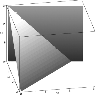
(a) Region of stability

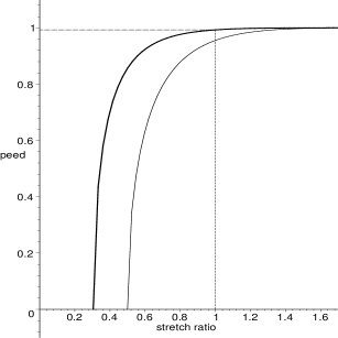
(b) Stoneley wave speed

Figure 1: Simple hyperelastic Bell materials ($\alpha^{*}/\rho^{*}=\alpha/\rho$, $\rho=8.2$, $\rho^{*}=3.2$).

Example 2: $\alpha^{*}/\rho^{*}=\textstyle{\frac{3}{2}}\alpha/\rho$, with $\rho=2$, $\rho^{*}=1$.

In this case, we have

$$\epsilon=\frac{\gamma^{*}}{\gamma}=\frac{\alpha^{*}}{\alpha}=\frac{3\rho^{*}}{2\rho}=\frac{3}{4}.$$ (60)

The limiting speed is

$$\hat{v}=v_{L}=\sqrt{\frac{\alpha}{\rho}}<v_{L}^{*}=\sqrt{\frac{\alpha^{*}}{\rho^{*}}}=\sqrt{\frac{3\alpha}{2\rho}},$$ (61)

and the corresponding $\eta$’s are

$$\eta_{L}=0,\quad\eta_{L}^{*}=\sqrt{1-\frac{\rho^{*}v_{L}^{2}}{\alpha^{*}}}=\sqrt{1-\frac{\rho^{*}\alpha}{\rho\alpha^{*}}}=\frac{1}{\sqrt{3}}.$$ (62)

The limiting condition (55) (with the starred and unstarred quantities interverted) is now satisfied for $\lambda_{1}$, $\lambda_{2}$ such that

$$(\sqrt{10+8\sqrt{3}}-\sqrt{3})\lambda_{1}-\lambda_{2}<0,\quad\text{or}\quad\lambda_{1}-0.31723\lambda_{2}<0.$$ (63)

Here we see that no interface wave may propagate when the materials are undeformed in the static state ($\lambda_{1}=\lambda_{2}=\lambda_{3}=1$), as noted by Stoneley [11] for linear isotropic incompressible materials with material parameters matching those of this example.

The other condition of existence of a Stoneley wave is the neutral condition (52), that is here

$$15\lambda_{1}-\lambda_{2}>0.$$ (64)

Figure 2(a) shows the intersection of the triangle $\lambda_{1}+\lambda_{2}+\lambda_{3}=3$ of possible values for the stretch ratios in Bell materials with the limiting condition (63) and with the neutral condition (64) for the combination of simple hyperelastic Bell materials in this example; the plane of the Figure coincides with the plane of the triangle. We see that the range of possible stretch ratios is far smaller here than in the previous example. For instance, in the case of plane strain $\lambda_{3}=1$, the stretch ratio $\lambda_{1}$ must belong to the (compressive) interval $]0.125,0.48167[$. Note that in this plane strain case, the Stoneley wave exists in a range where Rayleigh waves do not exist (in [5] it is proved that the domain of existence of Rayleigh waves in plane strain is: $\lambda_{1}\in]0.5,2[$.)

Figure 2(b) illustrates the influence of the loads on the Stoneley wave speed (thick curve) in the case of plane strain $\lambda_{3}=1$. The stretch ratio $\lambda_{1}$ is the coordinate on the horizontal axis. The speed, scaled with respect to the limiting wave speed $\hat{v}=\sqrt{\alpha/\rho}$, is the coordinate on the vertical axis; it is computed by solving numerically (4.1) for $y=v/\hat{v}$ with $\eta=\sqrt{1-y^{2}}$, $\eta^{*}=\sqrt{1-\textstyle{\frac{2}{3}}y^{2}}$, and $\gamma^{*}=\textstyle{\frac{3}{4}}\gamma$. Also represented are the Rayleigh wave speeds (thin curves) associated with each half-space, computed by solving numerically (4.1) for $y=v/\hat{v}$ with $\eta=\sqrt{1-y^{2}}$ and $\gamma^{*}=0$ (lower thin curve, with $y=1$ as an horizontal asymptote) or $\eta^{*}=\sqrt{1-\textstyle{\frac{2}{3}}y^{2}}$ and $\gamma=0$ (upper thin curve, with $y=\sqrt{\textstyle{\frac{3}{2}}}$ as an horizontal asymptote).

     

(a) Region of stability

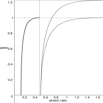
(b) Stoneley wave speed

Figure 2: Simple hyperelastic Bell materials ($\alpha^{*}/\rho^{*}=\textstyle{\frac{3}{2}}\alpha/\rho$, $\rho=2$, $\rho^{*}=1$).

4.2 Bell’s empirical model

For Bell’s empirical model materials [2], the strain energy functions of each half-space are

$$W_{\text{BEM}}=\textstyle{\frac{2}{3}}\nu_{0}[2(3-\lambda_{1}\lambda_{2}+\lambda_{2}\lambda_{3}+\lambda_{3}\lambda_{1})]^{\textstyle{\frac{3}{4}}},$$

$$W^{*}_{\text{BEM}}=\textstyle{\frac{2}{3}}\nu^{*}_{0}[2(3-\lambda_{1}\lambda_{2}+\lambda_{2}\lambda_{3}+\lambda_{3}\lambda_{1})]^{\textstyle{\frac{3}{4}}},$$ (65)

where $\nu_{0}$, $\nu^{*}_{0}$ are positive constants. For these models, the material response functions $\omega_{0}$, $\omega_{2}$, $\omega^{*}_{0}$ and $\omega^{*}_{2}$ provided by (2) are

$$\omega_{0}=\omega^{*}_{0}=0,\quad\omega_{2}=i_{3}^{-1}\nu_{0}[2(3-i_{2})]^{\textstyle{-\frac{1}{4}}},\quad\omega_{2}^{*}=\epsilon\omega_{2},\quad\epsilon=\nu_{0}^{*}/\nu_{0},$$ (66)

with $i_{2}$, $i_{3}$, given by (2.1)_3,4. Then $\alpha$, $\beta$, $\gamma$, $\alpha^{*}$, $\beta^{*}$, $\gamma^{*}$ are computed as:

$$\alpha=\frac{\lambda_{1}^{3}}{\lambda_{1}+\lambda_{2}}\omega_{2}=\frac{\lambda_{1}^{2}}{\lambda_{2}^{2}}\gamma,\quad\beta=\frac{\lambda_{1}^{2}}{2}\Big{[}2-\frac{(\lambda_{1}-\lambda_{2})^{2}}{4(3-i_{2})}\Big{]}\omega_{2}-\frac{\lambda_{1}^{2}\lambda_{2}}{\lambda_{1}+\lambda_{2}}\omega_{2},$$ (67)

$$\alpha^{*}=\epsilon\alpha,\quad\beta^{*}=\epsilon\beta,\quad\gamma^{*}=\epsilon\gamma.$$ (68)

Although the strain energy function of a “Bell’s empirical model” material depends only upon one material constant ($\nu_{0}$), as opposed to two ($\mathcal{C}_{1}$ and $\mathcal{C}_{2}$) for a “simple hyperelastic Bell” material, the full analysis of the Stoneley wave existence is too cumbersome and lengthy to be followed here. Indeed, we saw in §3.2 that the definition of the limiting speed depends on the sign of $2\beta-\alpha$ which, for these materials, is equal to

$$2\beta-\alpha=\omega_{2}\lambda_{1}^{2}[3\lambda_{1}^{3}-(12-5\lambda_{2})\lambda_{1}(\lambda_{1}+\lambda_{2})-\lambda_{2}^{3}]/[4(3-i_{2})(\lambda_{1}+\lambda_{2})].$$ (69)

The sign of this quantity (and hence the definition of $\hat{v}$) depends heavily on the values of the stretches $\lambda_{1}$ and $\lambda_{2}$ (For instance in the equibiaxial case $\lambda_{1}=\lambda_{3}$, we have $2\beta-\alpha=\omega_{2}\lambda_{1}^{2}(7\lambda_{1}-9)/[4(3-\lambda_{1})]$, which changes sign at $\lambda_{1}=\textstyle{\frac{9}{7}}$.) Consequently, the limiting condition is difficult to obtain in general. Moreover, the connection with Stoneley’s results [11] cannot be made because the parameters $\omega_{2}$, $\omega_{2}^{*}$ are singular when the material is isotropic (then $i_{2}=3$), where a different approach must be adopted [2].

Nevertheless, the neutral equation, which is independent of $\hat{v}$ and takes place away from isotropy, can be obtained and compared with Biot’s “stability equation” for rubber-like incompressible materials [8]. We deduce it by specializing (42) to the values (67) of $\alpha$, $\beta$, $\gamma$, $\alpha^{*}$, $\beta^{*}$, $\gamma^{*}$, as

$$\frac{4\lambda_{1}}{\lambda_{1}+\lambda_{2}}-\frac{(\lambda_{1}-\lambda_{2})^{2}}{4(3-i_{2})}-\Big{[}\frac{1-\epsilon}{1+\epsilon}\Big{]}^{2}\frac{(\lambda_{1}-\lambda_{2})^{2}}{\lambda_{1}(\lambda_{1}+\lambda_{2})}=0.$$ (70)

In the case of plane strain $\lambda_{3}=1$, the equation reduces to

$$(2\lambda_{1}-1)\lambda_{1}-2\Big{[}\frac{1-\epsilon}{1+\epsilon}\Big{]}^{2}(\lambda_{1}-1)^{2}=0.$$ (71)

Note that when $\epsilon=0$ in (70), only the lower half-space subsists and we recover the surface bifurcation criterion for Bell’s empirical materials in compression [12],

$$3-\frac{(\lambda_{1}-\lambda_{2})^{2}}{4(3-i_{2})}-\lambda_{1}^{-1}\lambda_{2}=0.$$ (72)

Figure 3 (where the plane of the Figure coincides with the plane of the triangle) shows the intersection between the triangle of possible stretch ratios for Bell materials and the neutral curve in the cases where $\epsilon=0.0$ [5] (thickest curve), $\epsilon=0.2$, $\epsilon=0.4$, $\epsilon=0.6$ (thinnest curve), and $\epsilon=0.8$ (dotted curve).

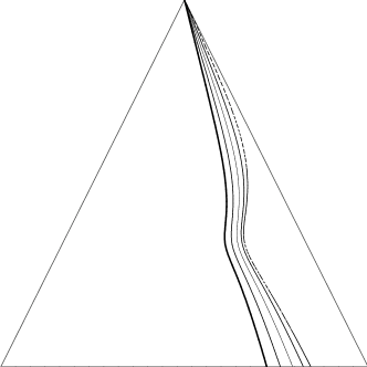
Figure 3: Neutral curves for ‘Bell empirical model’ materials.

4.3 Comparison with neo-Hookean incompressible materials

Biot [8] investigated the surface instability of incompressible materials under finite compression, and obtained the neutral condition, which he called the “characteristic equation for interfacial instability.” He then discussed the equation in the particular case of a neo-Hookean strain energy function,

$$W_{\text{nH}}=\mu_{0}(\lambda_{1}^{2}+\lambda_{2}^{2}+\lambda_{3}^{2}-3),$$ (73)

and expressed it, in the case of plane strain $\lambda_{3}=1$, as:

$$\lambda_{1}^{2}\Big{[}\frac{1+\lambda_{1}^{2}}{1-\lambda_{1}^{2}}\Big{]}^{2}=\Big{[}\frac{1-\epsilon}{1+\epsilon}\Big{]}^{2},\quad\epsilon=\frac{\mu_{0}}{\mu_{0}^{*}}.$$ (74)

He did not mention that the result was also valid for the neo-Hookean strain energy function,

$$W_{\text{MR}}=\mathcal{D}_{1}(\lambda_{1}^{2}+\lambda_{2}^{2}+\lambda_{3}^{2}-3)+\mathcal{D}_{2}(\lambda_{1}^{2}\lambda_{2}^{2}+\lambda_{2}^{2}\lambda_{3}^{2}+\lambda_{3}^{2}\lambda_{1}^{2}-3),$$ (75)

by replacing the rigidity ratio $\epsilon$ with

$$\epsilon=\frac{\mathcal{D}^{*}_{1}-\mathcal{D}^{*}_{2}}{\mathcal{D}_{1}-\mathcal{D}_{2}}.$$ (76)

Table 1 shows the numerical values of the critical stretches for the classes of Bell’s empirical model (2nd column), of neo-Hookean and Mooney-Rivlin incompressible materials (3rd column), and of simple hyperelastic Bell materials (4th column) in the case of plane strain, for different values of the rigidity ratio $\epsilon$. It appears that rubber can be compressed more than Bell’s empirical model but less than simple hyperelastic Bell materials, before the neutral equation is satisfied.

Table 1: Critical stretch ratios for interface instability ($\lambda_{3}=1$) $\epsilon$ Bell empirical rubber simple Bell 0.0 0.6667 0.5437 0.5000 0.2 0.6105 0.4457 0.4000 0.4 0.5625 0.3393 0.3000 0.6 0.5266 0.2257 0.2000 0.8 0.5060 0.1085 0.1000

Appendix

Strong ellipticity conditions for the incremental equations of motion in Bell materials.

For an unconstrained hyperelastic material maintained in a static state of pure homogeneous deformation, the incremental equations of motion are

$$\mathcal{A}_{jilk}u_{k,jl}=\rho u_{i,tt},$$ (1)

where $\mathcal{A}$ is the fourth-order instantaneous linear elasticity tensor. The nonzero components of $\mathcal{A}$ are:

$$\mathcal{A}_{iijj}=\lambda_{i}\lambda_{j}W_{ij},$$

$$\mathcal{A}_{ijij}=(\lambda_{i}W_{i}-\lambda_{j}W_{j})\lambda_{i}^{2}/(\lambda_{i}^{2}-\lambda_{j}^{2}),$$ (2)

$$\mathcal{A}_{ijji}=\mathcal{A}_{ijij}-\lambda_{i}W_{i},$$

(no sum) when the underlying deformation has distinct principal stretch ratios $\lambda_{1}$, $\lambda_{2}$, $\lambda_{3}$. The assumption of strong ellipticity for the equations of motion (1) imposes that

$$\mathcal{A}_{jilk}m_{j}n_{i}m_{l}n_{k}>0,\quad\text{for all nonzero}\quad\mathbf{m},\textbf{n}.$$ (3)

When the material is incompressible, $\text{det }\mathbf{V}=1$, where $\mathbf{V}$ is the left stretch tensor, and an arbitrary pressure $P$ is introduced [13]. Then the equations of motion are strongly elliptic for all values of $P$ when the inequalities (3) hold subject to

$$\mathbf{m}\cdot\mathbf{n}=0.$$ (4)

.

When the material is subject to the Bell constraint $\text{tr }\mathbf{V}=3$, an arbitrary scalar $p$ is introduced [2]. Then the equations of motion are strongly elliptic for all values of $p$ when the inequalities (3) hold subject to

$$\mathbf{m}\cdot\mathbf{Vn}=0.$$ (5)

The unit vectors

$$\mathbf{m}=\lambda_{1}^{-\textstyle{\frac{1}{2}}}\cos\theta\mathbf{i}+\lambda_{2}^{-\textstyle{\frac{1}{2}}}\sin\theta\mathbf{j},\quad\mathbf{n}=-\lambda_{1}^{-\textstyle{\frac{1}{2}}}\sin\theta\mathbf{i}+\lambda_{2}^{-\textstyle{\frac{1}{2}}}\cos\theta\mathbf{j},\quad 0\leq\theta\leq 2\pi,$$ (6)

are two such vectors, and the strong ellipticity condition says that

$$A\cos^{4}\theta+2B\sin^{2}\theta\cos^{2}\theta+C\sin^{4}\theta>0,$$ (7)

for all $\theta$, where $A$, $B$, $C$, are given by

$$A=\lambda_{1}^{-1}\lambda_{2}^{-1}\mathcal{A}_{1212},\quad C=\lambda_{1}^{-1}\lambda_{2}^{-1}\mathcal{A}_{2121},$$

$$B=(\lambda_{1}^{-2}\mathcal{A}_{1111}+\lambda_{2}^{-2}\mathcal{A}_{2222})/2-\lambda_{1}^{-1}\lambda_{2}^{-1}(\mathcal{A}_{1122}+\mathcal{A}_{1221}).$$ (8)

Choosing $\theta=\arctan(A/C)^{-\textstyle{\frac{1}{4}}}$, we arrive at $B+\sqrt{AC}>0$, which is equivalent to

$$\beta+\alpha>0,$$ (9)

where

$$\alpha=(W_{1}-W_{2})\lambda_{1}^{2}/[\lambda_{2}\lambda_{3}(\lambda_{1}^{2}-\lambda_{2}^{2})],$$

$$\beta=(W_{11}+W_{22}-2W_{12})\lambda_{1}/(2\lambda_{2}\lambda_{3})-\alpha\lambda_{2}/\lambda_{1}.$$ (10)

References

• [1] Beatty, M.F. and Hayes, M.A.: Deformations of an elastic, internally constrained material. Part 3: Small superimposed deformations and waves. Zeitschrift für angewandte Mathematik und Physik (ZAMP), 46, S72-S106 (1995).
• [2] Beatty, M.F.and Hayes, M.A.: Deformations of an elastic, internally constrained material. I. Homogeneous deformations. Journal of Elasticity, 29, 1-84 (1992).
• [3] Beatty, M.F. and Hayes, M.A.: Small amplitude torsional waves propagating in a Bell material, in Nonlinear Waves in Solids, pp.67-72, ed., J.L. Wegner & F.R. Norwood, ASME, New York, 1995.
• [4] Destrade, M.: Surface waves in deformed Bell materials. International Journal of Nonlinear Mechanics, 38, 809-814 (2002).
• [5] Destrade, M.: Rayleigh waves and surface stability of Bell materials in compression; comparison with rubber. Quarterly Journal of Mechanics and applied Mathematics, submitted.
• [6] Dowaikh, M.A. and Ogden, R.W.: Interfacial waves and deformations in pre-stressed elastic media. Proceedings of the Royal Society of London, A433, 313-328 (1991).
• [7] Chadwick, P.: Interfacial and surface waves in pre-strained isotropic elastic media. Zeitschrift für angewandte Mathematik und Physik (ZAMP), 46, S51-S71 (1995).
• [8] Biot, M.A.: Interfacial instability in finite elasticity under initial stress. Proceedings of the Royal Society of London, A273, 340-344 (1963).
• [9] Biot, M.A.: Mechanics of incremental deformations, John Wiley, New York (1965).
• [10] Barnett, D.M.; Lothe, J.; Gavazza, S.D.; Musgrave, M.J.P.: Considerations of the existence of interfacial (Stoneley) waves in bonded anisotropic elastic half-spaces. Proceedings of the Royal Society of London, A402, 153-166 (1985).
• [11] Stoneley, R.: Elastic waves at the surface of separation of two solids. Proceedings of the Royal Society of London, A106, 416-428 (1924).
• [12] Beatty, M.F. and Pan, F.X.: Stability of an internally constrained, hyperelastic slab. International Journal of Non-Linear Mechanics, 33, 867-906 (1998).
• [13] Chadwick, P.: The application of the Stroh formalism to prestressed elastic media. Mathematics and Mechanics of Solids, 2, 379-403 (1997).