Cellular buckling in I-section struts

Abstract

An analytical model that describes the interactive buckling of a thin-walled I-section strut under pure compression based on variational principles is presented. A formulation combining the Rayleigh–Ritz method and continuous displacement functions is used to derive a system of differential and integral equilibrium equations for the structural component. Numerical continuation reveals progressive cellular buckling (or snaking) arising from the nonlinear interaction between the weakly stable global buckling mode and the strongly stable local buckling mode. The resulting behaviour is highly unstable and when the model is extended to include geometric imperfections it compares excellently with some recently published experiments.

1 Introduction

The buckling of struts and columns represents the most common type of structural instability problem [1]. However, when the compression member is made from slender metallic plate elements they are well known to suffer from a variety of different elastic instability phenomena. In the current work, the classic problem of a strut under axial compression made from a linear elastic material with an open and doubly-symmetric cross-section – an “I-section” [2, 3] – is studied in detail using an analytical approach. Under this type of loading, long members are primarily susceptible to a global (or overall) mode of instability namely Euler buckling, where flexure about the weak axis occurs once the theoretical Euler buckling load is reached. However, when the individual plate elements of the strut cross-section, namely the flanges and the web, are relatively thin or slender, elastic local buckling of these may also occur; if this happens in combination with the global instability, then the resulting behaviour is usually far more unstable than when the modes are triggered individually. Recent work on the interactive buckling of struts include experimental and finite element studies [4, 5], where the focus was on the behaviour of struts made from stainless steel. However, the more generic finding that the members had an increased sensitivity to imperfections was highlighted. Other structural components that are known to suffer from the interaction of local and global instability modes are thin-walled beams under uniform bending [6], sandwich struts [7, 8], stringer-stiffened and corrugated plates [9, 10] and built-up, compound or reticulated columns [11].

Apart from the aforementioned work where some numerical modelling was presented [5], the formulation of a mathematical model accounting for the nonlinear interactive buckling behaviour has not been forthcoming. The current work presents the development of a variational model that accounts for the mode interaction between global Euler buckling and local buckling of a flange such that the perfect and imperfect elastic post-buckling response of the strut can be evaluated. A system of nonlinear ordinary differential equations subject to integral constraints is derived and is solved using the numerical continuation package Auto [12]. It is indeed found that the system is highly unstable when interactive buckling is triggered; snap-backs in the response, showing sequential destabilization and restabilization and a progressive spreading of the initial localized buckling mode, are also revealed. This latter type of response has become known in the literature as cellular buckling [13] or snaking [14] and it is shown to appear naturally in the numerical results of the current model. As far as the authors are aware, this is the first time this phenomenon has been captured analytically in struts undergoing Euler and local buckling simultaneously. Similar behaviour has been discovered in various other mechanical systems such as in the post-buckling of cylindrical shells [15], the sequential folding of geological layers [16] and most recently in the lateral buckling of thin-walled beams under pure bending [6].

Experimental results from the literature [4, 17] are used for validation purposes. The mechanical destabilization and the nature of the post-buckling deformation compare excellently with the current model. This demonstrates that the fundamental physics of this system is captured by the analytical approach both qualitatively and quantitatively. A brief discussion is presented on how the current model could be enhanced and then conclusions are drawn.

2 Analytical Model

Consider a thin-walled I-section strut of length $L$ made from a linear elastic, homogeneous and isotropic material with Young’s modulus $E$ and Poisson’s ratio $\nu$. It is loaded by an axial force $P$ that is applied at the centroid of the cross-section, as shown in Figure 1(a) and (b) respectively,

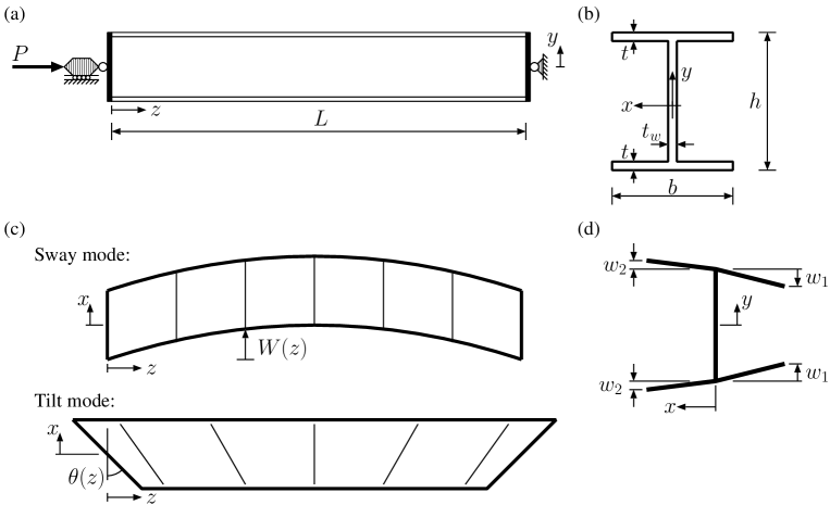
Figure 1: (a) Elevation of an I-section strut of length $L$ that is compressed axially by a force $P$. The lateral and longitudinal coordinates are $y$ and $z$ respectively. (b) Cross-section of strut; the transverse coordinate is $x$. (c) Sway and tilt components of the minor axis global buckling mode. (d) Local buckling mode: out-of-plane flange displacement functions $w_{i}(x,z)$; note the linear distribution in the $x$ direction.

with rigid end plates that transfer the force uniformly to the entire cross-section. The web is assumed to provide a simple support to both flanges and not to buckle locally under the axial compression, an assumption that is justified later. In the current study, the total cross-section depth is $h$ with each flange having width $b$ and thickness $t$. It is assumed currently that the I-section is effectively made up from two channel members connected back-to-back; hence, the assumption is that the web thickness $t_{w}=2t$, a type of arrangement that has been used in recent experimental studies [4, 6, 17]. The strut length $L$ is varied such that in one case, which is presented later, Euler buckling about the weaker $y$-axis occurs before any flange buckles locally and in the other case the reverse is true – flange local buckling is critical.

The formulation begins with the definitions for both the global and the local modal displacements. Timoshenko beam theory is assumed, meaning that the effect of shear is not neglected as in standard Euler–Bernoulli beam theory. Although it turns out that the effect of shear is only minor, it is necessary to account for it since it provides the key terms within the total potential energy that allow buckling mode interaction to be modelled [6, 7]. To account for shear, two generalized coordinates $q_{s}$ and $q_{t}$, defined as the amplitudes of the degrees of freedom known as “sway” and “tilt” [7] are introduced to model the global mode, as shown in Figure 1(c), where the lateral displacement $W$ and the rotation $\theta$ are given by the following expressions:

$$W(z)=q_{s}L\sin\frac{\pi z}{L},\quad\theta(z)=q_{t}\pi\cos\frac{\pi z}{L}.$$ (1)

For the present case, the shear strain in the $xz$ plane, $\gamma_{xz}$, is included and is given by the following expression:

$$\gamma_{xz}=\frac{\mbox{$\,\mathrm{d}$}W}{\mbox{$\,\mathrm{d}$}z}-\theta=\left(q_{s}-q_{t}\right)\pi\cos\frac{\pi z}{L}.$$ (2)

Of course, Euler–Bernoulli beam theory would imply that since $\gamma_{xz}=0$, then $q_{s}=q_{t}$.

The local mode is modelled with appropriate boundary conditions. Moreover, the possibility of a distinct local buckling mode occurring before global buckling implies that the entire flange may deflect. However, if the interaction between local and global modes occurs then the symmetry of the local buckling mode would be broken and the flanges would not buckle with the same displacement. Hence, two separate lateral displacement functions $w_{1}$ and $w_{2}$ need to be defined, as shown in Figure 1(d), to allow for the break in symmetry. Since the outstands of the flanges have free edges, whereas the web is assumed to provide no more than a simple support to the flanges, a linear distribution is assumed in the $x$ direction; Bulson [18] showed this distribution is correct for the local buckling eigenmode for that type of rectangular plate. For the local mode in-plane displacements $u_{i}$, the distributions are also assumed to be linear in $x$, as shown in Figure 2.

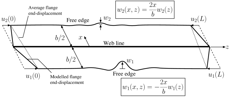
Figure 2: Displacement functions of local buckling mode in flanges. Longitudinal and lateral flange displacements $u_{i}(x,z)$ and $w_{i}(x,z)$ respectively. Note the linear distributions in $x$ direction and the average end-displacement, as opposed to the modelled flange end-displacement, which is used to calculate the local contribution to the work done.

This is in fact another consequence of the Timoshenko beam theory assumption where plane sections are assumed to remain plane. These assumptions lead to the following expressions for the local out-of-plane displacements $w_{i}$ with the in-plane displacements $u_{i}$:

$$w_{i}(x,z)=(-1)^{i}\left(\frac{2x}{b}\right)w_{i}(z),\quad u_{i}(x,z)=(-1)^{i}\left(\frac{2x}{b}\right)u_{i}(z),$$ (3)

where $i=\{1,2\}$ throughout the current article. The transverse in-plane displacement $v(z,x)$ is assumed to be small and is hence neglected for the current case; this reflects the findings from Koiter and Pignataro [9] for rectangular plates with three pinned edges and one free edge.

Since, in practice, perfect geometries do not exist, an initial out-of-straightness in the $x$-direction, $W_{0}$, is introduced as a global imperfection to the web and flanges in the current model. An initial rotation of the plane section $\theta_{0}$ is also introduced to simulate the out-of-straightness in the flanges. The expressions for $W_{0}$ and $\theta_{0}$ are given by:

$$W_{0}=q_{s0}L\sin\frac{\pi z}{L},\quad\theta_{0}=q_{t0}\pi\cos\frac{\pi z}{L},$$ (4)

and are analogous to Equation (1). Note that the assumption of Timoshenko beam theory implies that shear strains in the $xz$ plane due to the initial imperfection are also introduced.

2.1 Total potential energy

The total potential energy, $V$, was determined with the main contributions being the global and local bending energy $U_{bo}$ and $U_{bl}$ respectively, the membrane energy $U_{m}$, and the work done $P\mathcal{E}$. Note that the global bending energy $U_{bo}$ only comprises the bending energy stored in the web, since the membrane energy stored in the flanges accounts for the effect of bending in the flanges through the tilt mode. The initial out-of-straightness $W_{0}(z)$ is stress-relieved [19, 20], implying that the elemental moment $M$ drops to zero as illustrated in Figure 3(a).

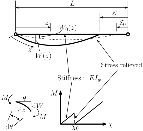
Figure 3: Introduction of geometric imperfections $W_{0}$ and $\theta_{0}$ in (a) the web and (b) the flanges.

The global bending energy involves the second derivative of $W$ and $W_{0}$ and is hence given by:

$$U_{bo}=\frac{1}{2}EI_{w}\int_{0}^{L}\left(\ddot{W}-\ddot{W_{0}}\right)^{2}\mbox{$\,\mathrm{d}$}z=\frac{1}{2}EI_{w}\int_{0}^{L}\left(q_{s}-q_{s0}\right)^{2}\frac{\pi^{4}}{L^{2}}\sin^{2}\frac{\pi z}{L}\mbox{$\,\mathrm{d}$}z,$$ (5)

where dots represent differentiation with respect to $z$ and $I_{w}=t_{w}^{3}(h-2t)/12$ is the second moment of area of the web about the global weak axis. Obviously, for the case where $t_{w}=2t$, the expression becomes $I_{w}=2t^{3}(h-2t)/3$. The local bending energy, accounting for both flanges, is determined as:

$$U_{bl} =D\int_{0}^{L}\left[\int_{-b/2}^{0}B_{1}\mbox{$\mathrm{d}$}x+\int_{0}^{b/2}B_{2}\mbox{$\mathrm{d}$}x\right]\mbox{$\mathrm{d}$}z$$ (6)

$$=D\int_{0}^{L}\left[\frac{b}{6}\left(\ddot{w}_{1}^{2}+\ddot{w}_{2}^{2}\right)+\frac{4\left(1-\nu\right)}{b}\left(\dot{w}_{1}^{2}+\dot{w}_{2}^{2}\right)\right]\mbox{$\mathrm{d}$}z,$$

where $B_{i}$, the contribution from $w_{i}$ to the standard expression for the incremental strain energy from bending a plate [1], is given by:

$$B_{i}=\left(\frac{\partial^{2}w_{i}}{\partial z^{2}}+\frac{\partial^{2}w_{i}}{\partial x^{2}}\right)^{2}-2\left(1-\nu\right)\left[\frac{\partial^{2}w_{i}}{\partial z^{2}}\frac{\partial^{2}w_{i}}{\partial x^{2}}-\left(\frac{\partial^{2}w_{i}}{\partial z\partial x}\right)^{2}\right],$$ (7)

with $D=Et^{3}/[12(1-\nu^{2})]$ being the plate flexural rigidity. The buckled configuration of the flange plate involves double curvature in the $x$ and $z$ directions, indicating the non-developable nature of plate deformation. The so-called membrane strain energy ($U_{m}$) is derived from considering the direct strains ($\varepsilon$) and the shear strains ($\gamma$) in the flanges thus:

$$U_{m}=U_{d}+U_{s}=\int_{0}^{L}\left[\int_{-h/2}^{-h/2+t}F\mbox{$\,\mathrm{d}$}y+\int_{h/2-t}^{h/2}F\mbox{$\,\mathrm{d}$}y\right]\mbox{$\mathrm{d}$}z,$$ (8)

where:

$$\begin{split}F=\frac{1}{2}&\biggl{\{}\int_{-b/2}^{0}\left[E\left(\varepsilon^{2}_{z1}+\varepsilon^{2}_{x1}+2\nu\varepsilon_{z1}\varepsilon_{x1}\right)+G\gamma^{2}_{xz1}\right]\mbox{$\mathrm{d}$}x\\ &\quad+\int_{0}^{b/2}\left[E\left(\varepsilon^{2}_{z2}+\varepsilon^{2}_{x2}+2\nu\varepsilon_{z2}\varepsilon_{x2}\right)+G\gamma^{2}_{xz2}\right]\mbox{$\mathrm{d}$}x\biggl{\}}.\end{split}$$ (9)

The transverse component of strain $\varepsilon_{xi}$ is neglected since it has been shown that it has no effect on the post-buckling behaviour of a long plate with three simply-supported edges and one free edge [9]. The longitudinal strain $\varepsilon_{z}$ has to be modelled separately for different outstand flanges. Recall that the tilt component of the in-plane displacement from the global mode, including the initial imperfection, is given by $u_{t}=-(\theta-\theta_{0})x$ as shown in Figure 3(b); hence:

$$\varepsilon_{z,\mathrm{global}}=\frac{\partial u_{t}}{\partial z}=x\left(q_{t}-q_{t0}\right)\frac{\pi^{2}}{L}\sin\frac{\pi z}{L}.$$ (10)

The local mode contribution is based on von Kármán plate theory. A pure in-plane compressive strain $\Delta$ is also included. The direct strains in the compression and tension side of the flanges, denoted as $\varepsilon_{z1}$ and $\varepsilon_{z2}$ respectively, are given by the general expression:

$$\varepsilon_{zi} =\varepsilon_{z,\mathrm{global}}-\Delta+\frac{\partial u_{i}}{\partial z}+\frac{1}{2}\left(\frac{\partial w_{i}}{\partial z}\right)^{2}$$ (11)

$$=x\left(q_{t}-q_{t0}\right)\frac{\pi^{2}}{L}\sin\frac{\pi z}{L}-\Delta+(-1)^{i}\left(\frac{2x}{b}\right)\dot{u_{i}}+\frac{2x^{2}}{b^{2}}\dot{w}_{i}^{2}.$$

The strain energy from direct strains ($U_{d}$) is thus, assuming that $h\gg t$:

$$U_{d}=Etb\int_{0}^{L} \biggl{\{}\frac{b^{2}}{12}\left(q_{t}-q_{t0}\right)^{2}\frac{\pi^{4}}{L^{2}}\sin^{2}\frac{\pi z}{L}+\Delta^{2}+\frac{1}{6}\left({\dot{u}_{1}}^{2}+{\dot{u}_{2}}^{2}\right)+\frac{1}{40}\left({\dot{w}_{1}}^{4}+{\dot{w}_{2}}^{4}\right)$$ (12)

$$-\left(q_{t}-q_{t0}\right)\frac{b\pi^{2}}{2L}\sin\frac{\pi z}{L}\left[\frac{1}{3}\left({\dot{u}}_{1}-{\dot{u}}_{2}\right)+\frac{1}{8}\left({\dot{w}_{1}}^{2}-{\dot{w}_{1}}^{2}\right)\right]-\frac{1}{2}\Delta\left(\dot{u}_{1}+\dot{u}_{2}\right)$$

$$-\frac{1}{6}\Delta\left({\dot{w}_{1}}^{2}+{\dot{w}_{2}}^{2}\right)+\frac{1}{8}\left(\dot{u}_{1}{\dot{w}_{1}}^{2}+\dot{u}_{2}{\dot{w}_{2}}^{2}\right)+\frac{h}{b}\Delta^{2}\biggr{\}}\mbox{$\,\mathrm{d}$}z,$$

where, apart from the final term which represents the energy stored in the web, the contributions are from the direct strains in both flanges. The shear strain energy $U_{s}$ contains the shear modulus $G$, which is given by $E/[2(1+\nu)]$ for a homogeneous and isotropic material. The shear strain $\gamma_{xz}$ contributions are also modelled separately for the compression and the tension side of the flanges. The expression for each outstand is given by the general expression:

$$\gamma_{xzi} =\frac{\partial}{\partial z}\left(W-W_{0}\right)-\left(\theta-\theta_{0}\right)+\frac{\partial u_{i}}{\partial x}+\frac{\partial w_{i}}{\partial z}\frac{\partial w_{i}}{\partial x}$$ (13)

$$=\left(q_{s}-q_{t}-q_{s0}+q_{t0}\right)\pi\cos\frac{\pi z}{L}+(-1)^{i}\left(\frac{2}{b}\right)u_{i}+\frac{4x}{b^{2}}w_{i}\dot{w_{i}}.$$

The expression for the strain energy from shear is thus:

$$U_{s}=Gtb\int_{0}^{L} \biggl{[}\left(q_{s}-q_{t}-q_{s0}+q_{t0}\right)^{2}\pi^{2}\cos^{2}\frac{\pi z}{L}$$ (14)

$$-\left(q_{s}-q_{t}-q_{s0}+q_{t0}\right)\frac{\pi}{b}\cos\frac{\pi z}{L}\left(2u_{1}-2u_{2}+w_{1}\dot{w}_{1}-w_{2}\dot{w}_{2}\right)$$

$$+\frac{2}{b^{2}}\left({u_{1}}^{2}+{u_{2}}^{2}+\frac{1}{3}{w_{1}}^{2}{\dot{w}_{1}}^{2}+\frac{1}{3}{w_{2}}^{2}{\dot{w}_{2}}^{2}+u_{1}w_{1}\dot{w}_{1}+u_{2}w_{2}\dot{w}_{2}\right)\biggr{]}\mbox{$\mathrm{d}$}z.$$

Finally, the work done by the axial load $P$ is given by:

$$P\mathcal{E}=\frac{P}{2}\int_{0}^{L}\left[q_{s}^{2}\pi^{2}\cos^{2}\frac{\pi z}{L}-\left(\dot{u}_{1}+\dot{u}_{2}\right)+2\Delta\right]\mbox{$\mathrm{d}$}z,$$ (15)

where $\mathcal{E}$ comprises the longitudinal displacement due to global buckling, the in-plane displacement due to local buckling and the initial end shortening. Note that the displacement due to local buckling is taken as the average value between the maximum in-plane displacement in the more compressed outstand $u_{1}$ and the maximum in-plane displacement in the less compressed outstand $u_{2}$, which is illustrated in Figure 2. Moreover, the possible term in $q_{s0}$ has been neglected since it would vanish on differentiation for equilibrium anyway. The total potential energy $V$ is therefore assembled thus:

$$V=U_{bo}+U_{bl}+U_{m}-P\mathcal{E}.$$ (16)

2.2 Variational Formulation

The governing differential equations are obtained by performing the calculus of variations on the total potential energy $V$ following a well established procedure that has been detailed in [7]. The integrand of the total potential energy $V$ can be expressed as the Lagrangian ($\mathcal{L}$) of the form:

$$V=\int_{0}^{L}\mathcal{L}\left(\ddot{w}_{i},\dot{w}_{i},w_{i},\dot{u}_{i},u_{i},z\right)\mbox{$\,\mathrm{d}$}z.$$ (17)

The first variation of $V$, which is denoted as $\delta V$, is given by:

$$\delta V=\int_{0}^{L}\left[\frac{\partial\mathcal{L}}{\partial\ddot{w}_{i}}\delta\ddot{w}_{i}+\frac{\partial\mathcal{L}}{\partial\dot{w}_{i}}\delta\dot{w}_{i}+\frac{\partial\mathcal{L}}{\partial w_{i}}\delta w_{i}+\frac{\partial\mathcal{L}}{\partial\dot{u}_{i}}\delta\dot{u}_{i}+\frac{\partial\mathcal{L}}{\partial u_{i}}\delta u_{i}\right]\mbox{$\,\mathrm{d}$}z.$$ (18)

To find the equilibrium states, $V$ must be stationary, which requires $\delta V$ to vanish for any small change in $w_{i}$ and $u_{i}$. By assuming that $\delta\ddot{w}_{i}=\mbox{$\mathrm{d}$}(\delta\dot{w}_{i})/\mbox{$\,\mathrm{d}$}z$, $\delta\dot{w}_{i}=\mbox{$\mathrm{d}$}(\delta w_{i})/\mbox{$\mathrm{d}$}z$ and similarly $\delta\dot{u}_{i}=\mbox{$\mathrm{d}$}(\delta u_{i})/\mbox{$\mathrm{d}$}z$, integration by parts allows the development of the Euler–Lagrange equations for $w_{i}$ and $u_{i}$; these comprise fourth order ordinary differential equations (ODEs) in terms of $w_{i}$ and second order ODEs in terms for $u_{i}$. For the equations to be solved by the continuation package Auto, the system variables need to be rescaled with respect to the non-dimensional spatial coordinate $\tilde{z}=2z/L$. Non-dimensional out-of-plane displacements $\tilde{w}_{i}$ and in-plane displacements $\tilde{u}_{i}$ are also introduced as $2w_{i}/L$ and $2u_{i}/L$ respectively. Note that these scalings assume symmetry about the midspan and the differential equations are solved for half the length of the strut; this assumption has been shown to be perfectly acceptable for cases where the global buckling is critical [20]. For cases where local buckling is critical, this condition is also acceptable so long as the length of the strut $L$ is much larger than the flange outstand width $b/2$; hence the critical loads for symmetric and antisymmetric modes are sufficiently close for the buckling plate. The non-dimensional differential equations for $w_{i}$ and $u_{i}$ are thus:

$$\begin{split}\tilde{\ddddot{w_{i}}}&-6\phi^{2}\left(1-\nu\right)\tilde{\ddot{w}}_{i}-(-1)^{i}\left(\frac{3\tilde{D}}{8}\right)\biggl{\{}\left(q_{t}-q_{t0}\right)\frac{\pi^{2}}{4\phi}\left(\sin\frac{\pi\tilde{z}}{2}\tilde{\ddot{w}}_{i}+\frac{\pi}{2}\cos\frac{\pi\tilde{z}}{2}\tilde{\dot{w}}_{i}\right)\\ &-(-1)^{i}\biggl{[}\tilde{\ddot{w}}_{i}\left(\frac{2}{3}\Delta-\frac{3}{5}\tilde{\dot{w}}_{i}^{2}\right)-\frac{1}{2}\left(\tilde{\ddot{u}}_{i}\tilde{\dot{w}}_{i}+\tilde{\dot{u}}_{i}\tilde{\ddot{w}}_{i}\right)\biggr{]}\biggr{\}}\\ &-\frac{3\tilde{G}}{8}\phi^{2}\tilde{w}_{i}\biggl{[}\frac{2}{3}{\tilde{\dot{w}}_{i}^{2}}+\frac{2}{3}{\tilde{w}_{i}}\tilde{\ddot{w}}_{i}+\tilde{\dot{u}}_{i}-(-1)^{i}\left(q_{s}-q_{t}-q_{s0}+q_{t0}\right)\frac{\pi^{2}}{2\phi}\sin\frac{\pi\tilde{z}}{2}\biggr{]}=0,\\ \end{split}$$ (19)

$$\begin{split}\tilde{\ddot{u}}_{i}&+\frac{3}{4}\tilde{\dot{w}}_{i}\tilde{\ddot{w}}_{i}+(-1)^{i}\biggl{\{}\left(q_{t}-q_{t0}\right)\frac{\pi^{3}}{4\phi}\cos\frac{\pi\tilde{z}}{2}\\ &-\left(\frac{3\tilde{G}\phi^{2}}{\tilde{D}}\right)\biggl{[}\left(q_{s}-q_{t}-q_{s0}+q_{t0}\right)\frac{\pi}{\phi}\cos\frac{\pi\tilde{z}}{2}+(-1)^{i}\left(\frac{1}{2}\tilde{w}_{i}\tilde{\dot{w}}_{i}+\tilde{u}_{i}\right)\biggr{]}\biggl{\}}=0,\\ \end{split}$$ (20)

where $i=\{1,2\}$ again along with $\tilde{D}=EtL^{2}/D$, $\tilde{G}=GtL^{2}/D$ and $\phi=L/b$. Equilibrium also requires the minimization of the total potential energy with respect to the generalized coordinates $q_{s}$, $q_{t}$ and $\Delta$. This essentially provides three integral conditions, in non-dimensional form:

$$\begin{split}\frac{\partial V}{\partial q_{s}}&=\pi^{2}\left(q_{s}-q_{s0}\right)+\tilde{s}\left(q_{s}-q_{t}-q_{s0}+q_{t0}\right)-\frac{PL^{2}}{EI_{w}}q_{s}\\ &\quad-\frac{\tilde{s}\phi}{\pi}\int_{0}^{1}\cos\frac{\pi\tilde{z}}{2}\left[\frac{1}{2}\left(\tilde{w}_{1}\tilde{\dot{w}}_{1}-\tilde{w}_{2}\tilde{\dot{w}}_{2}\right)+\left(\tilde{u}_{1}-\tilde{u}_{2}\right)\right]\mbox{$\mathrm{d}$}\tilde{z}=0,\\ \frac{\partial V}{\partial q_{t}}&=\pi^{2}\left(q_{t}-q_{t0}\right)-\tilde{t}\left(q_{s}-q_{t}-q_{s0}+q_{t0}\right)+\phi\int_{0}^{1}\biggl{\{}\frac{\tilde{t}}{\pi}\cos\frac{\pi\tilde{z}}{2}\biggl{[}\frac{1}{2}\left(\tilde{w}_{1}\tilde{\dot{w}}_{1}-\tilde{w}_{2}\tilde{\dot{w}}_{2}\right)\\ &\qquad+\left(\tilde{u}_{1}-\tilde{u}_{2}\right)\biggr{]}-\sin\frac{\pi\tilde{z}}{2}\left[2\left(\tilde{\dot{u}}_{1}-\tilde{\dot{u}}_{2}\right)+\frac{3}{4}\left({\tilde{\dot{w}}_{1}^{2}}-{\tilde{\dot{w}}_{2}^{2}}\right)\right]\biggr{\}}\mbox{$\mathrm{d}$}\tilde{z}=0,\\ \frac{\partial V}{\partial\Delta}&=\int_{0}^{1}\left[2\left(1+\frac{h}{b}\right)\Delta-\frac{1}{2}\left(\tilde{\dot{u}}_{1}+\tilde{\dot{u}}_{2}\right)-\frac{1}{6}\left(\tilde{\ddot{w}}_{1}^{2}+\tilde{\ddot{w}}_{2}^{2}\right)-\frac{P}{Etb}\right]\mbox{$\mathrm{d}$}\tilde{z}=0,\end{split}$$ (21)

where $\tilde{s}=2GtbL^{2}/(EI_{w})$ and $\tilde{t}=12G\phi^{2}/E$. Since the strut is an integral member, the expressions in Equation (21) provide a relationship linking $q_{s}$ and $q_{t}$ before any interactive buckling occurs, i.e. when $w_{i}=u_{i}=0$. This relationship is assumed to hold also between $q_{s0}$ and $q_{t0}$, which has the beneficial effect of reducing the number of imperfection amplitude parameters to one. The relationship between $q_{s0}$ and $q_{t0}$ is given by:

$$q_{s0}=\left(\frac{\pi^{2}}{\tilde{t}}+1\right)q_{t0}.$$ (22)

The boundary conditions for $\tilde{w}_{i}$ and $\tilde{u}_{i}$ and their derivatives are for pinned end conditions for $\tilde{x}=0$ and for symmetry at $\tilde{x}=1$:

$$\tilde{w}_{i}(0)=\tilde{\ddot{w}}_{i}(0)=\tilde{\dot{w}}_{i}(1)=\tilde{\dddot{w}}_{i}(1)=\tilde{u}_{i}(1)=0,$$ (23)

with further conditions from matching the in-plane strain:

$$\frac{1}{3}\tilde{\dot{u}}_{i}(0)+\frac{1}{8}\tilde{\dot{w}}_{i}^{2}(0)-\frac{1}{2}\Delta+\frac{P}{2Etb}=0.$$ (24)

Linear eigenvalue analysis for the perfect strut ($q_{s0}=q_{t0}=0$) is conducted to determine the critical load for global buckling $P_{o}^{\mathrm{C}}$. This is achieved by considering that the Hessian matrix $\mathbf{V}_{st}$ at the critical load is singular. Hence:

$$\mathrm{det}\left(\mathbf{V}_{st}\right)=\left|\begin{array}[]{cc}\frac{\partial^{2}V}{\partial q_{s}^{2}}&\frac{\partial^{2}V}{\partial q_{s}\partial q_{t}}\\ \frac{\partial^{2}V}{\partial q_{t}\partial q_{s}}&\frac{\partial^{2}V}{\partial q_{t}^{2}}\end{array}\right|=0,$$ (25)

Recalling of course that in fundamental equilibrium for this case, $q_{s}=q_{t}=w_{i}=u_{i}=0$. Hence, the critical load for global buckling is:

$$\mbox{$P_{o}^{\mathrm{C}}$}=\frac{\pi^{2}EI_{w}}{L^{2}}+\frac{2Gtb}{1+\tilde{t}/\pi^{2}}.$$ (26)

If the limit $G\rightarrow\infty$ is taken, which represents a principal assumption in Euler–Bernoulli bending theory, the critical load expression converges to the Euler buckling load for an I-section strut buckling about the weak axis.

3 Numerical examples of perfect behaviour

The full nonlinear differential equations are obviously complicated to be solved analytically. The continuation and bifurcation software Auto-07p [12] has been shown in the literature [6, 7] to be an ideal tool to solve the equations numerically. For this type of mechanical problem, one of its major attributes is that it has the capability to show the evolution of the solutions to the equations with parametric changes. The solver is very powerful in locating bifurcation points and tracing branching paths as model parameters are varied. To demonstrate this, an example set of cross-section and material properties are chosen which are shown in Table 1.

Flange width $b$	$96~{}\mbox{$\mathrm{mm}$}$
Flange thickness $t$	$1.2~{}\mbox{$\mathrm{mm}$}$
Cross-section depth $h$	$120~{}\mbox{$\mathrm{mm}$}$
Cross-section area $A$	$513~{}\mbox{$\mathrm{mm}$}^{2}$
Young’s modulus $E$	$210~{}\mathrm{kN/mm^{2}}$
Poisson’s ratio $\nu$	0.3

Table 1: Cross-section and material properties of an example strut. Recall that the thickness of the web $t_{w}=2t$. The geometric properties are similar to those tested in [4]. The length $L$ is varied such that the cases where global buckling or local buckling are critical can be presented.

In this example, perfect behaviour is assumed and hence $W_{0}=\theta_{0}=0$. The global critical load $P_{o}^{\mathrm{C}}$ can be calculated using Equation (26), whereas an estimate for the local buckling critical stress $\sigma_{l}^{\mathrm{C}}$ can be evaluated using the well-known plate buckling formula $\sigma_{l}^{\mathrm{C}}=kD\pi^{2}/(b^{2}t)$, where the coefficient $k$ depends on the boundary conditions; approximate values of $k=0.426$ and $k=4$ are chosen for the rectangular plates representing the flange outstands (three edges pinned and one edge free) and the web (all four edges pinned) respectively, assuming that the plates are relatively long [18]. Table 2

$L~{}(\mathrm{m})$	$\sigma_{o}^{\mathrm{C}}~{}(\mathrm{N/mm^{2}})$	$\sigma_{l,\mathrm{flange}}^{\mathrm{C}}~{}(\mathrm{N/mm^{2}})$	$\sigma_{l,\mathrm{web}}^{\mathrm{C}}~{}(\mathrm{N/mm^{2}})$	Critical mode
$3.5$	$58.3$	$51.1$	$2731$	Local (flange)
$4.0$	$44.7$	$51.1$	$2731$	Global

Table 2: Theoretical values of the global and local critical buckling stresses for two separate lengths. The expression for $\sigma_{o}^{\mathrm{C}}=\mbox{$P_{o}^{\mathrm{C}}$}/A$ and the web is obviously not vulnerable to local buckling.

summarizes the critical stresses and shows that the assigned cross-section dimensions satisfy the assumptions that the local mode is critical for one of the lengths and the global mode is critical for the other. Moreover, the critical stress of the web is orders of magnitude higher than that of the flange, which justifies the assumption stated earlier. It should be emphasized that the local buckling critical stress is calculated numerically in Auto and is usually marginally higher than the value given in Table 2, with an error not exceeding $5\%$ with the theoretical expressions given above for the long plates.

Numerical continuation was performed in Auto for the cases where local buckling and global buckling were critical in turn. The principal parameters used in the continuation process were interchangeable, but generally $q_{s}$ was varied for computing the equilibrium paths for the distinct buckling modes and $P$ was varied for evaluating the interactive buckling paths. For the case of local buckling being critical, the continuation process initiated from zero load with the local buckling critical load $P_{l}^{\mathrm{C}}$ being obtained numerically. The post-buckling path was then computed by using the branch switching facility within the software and the distinct local buckling equilibrium path was computed until a secondary bifurcation point $\mathrm{S}$ was found. It was from this point that the interactive buckling path was found, again through the use of branch switching. For the case where global buckling was critical, since the critical load was determined analytically in Equation (26), the initial post-buckling path was computed first from $P_{o}^{\mathrm{C}}$ and many bifurcation points were detected on the weakly stable post-buckling path; the focus being on the one with the lowest value of $q_{s}$, the secondary bifurcation point $\mathrm{S}$. A subsequent run was then necessary starting from $\mathrm{S}$ using the branch switching function, after which the equilibrium path again exhibits the interaction between the global and the local modes. Figure 4 shows the procedures for the cases diagrammatically with (a–b) concerning the perfect cases discussed above and (c), the imperfect case, is considered later in the section on validation.

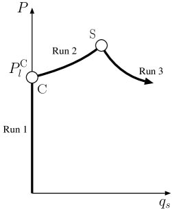
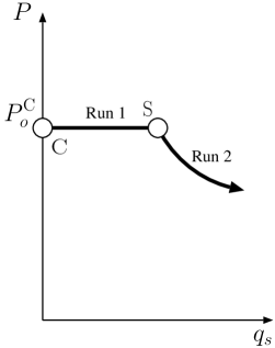
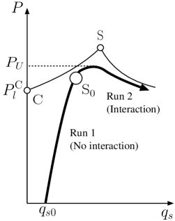
Figure 4: Numerical continuation procedures. (a) Local buckling being critical; (b) Global buckling being critical; (c) Imperfect case – example of local buckling being critical shown. The thicker line shows the actual solution path in each of the examples shown. Points $\mathrm{C}$ and $\mathrm{S}$ represent the critical and secondary bifurcations respectively, whereas the point $\mathrm{S}_{0}$ represents the bifurcation leading to interactive buckling in the imperfect case with the load $P_{U}$ being the ultimate load in the imperfect case.

3.1 Local buckling critical

In this section, the strut with properties given in Table 1 with length $L$ being $3.5~{}\mathrm{m}$ is analysed, where the flanges buckle locally first. Figure 5

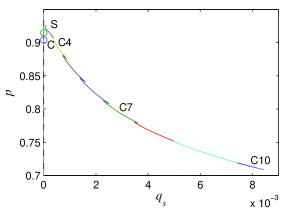
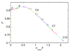
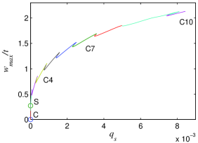
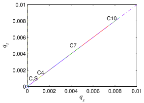
Figure 5: Numerical equilibrium paths for $L=3.5~{}\mathrm{m}$ where local buckling is critical. Graphs of the normalized force ratio $p$ versus (a) the generalized coordinate $q_{s}$ and (b) the maximum out-of-plane displacement of the buckled flange plate, in non-dimensional form, $w_{\mathrm{max}}/t$ are shown. (c) shows $w_{\mathrm{max}}/t$ versus $q_{s}$ and (d) shows the relationship between the generalized coordinates $q_{s}$ and $q_{t}$ defining the global buckling mode during interactive buckling, with the dot-dash line showing the Euler–Bernoulli bending condition $q_{s}=q_{t}$.

shows a plot of the normalized axial load $p=P/\mbox{$P_{o}^{\mathrm{C}}$}$ versus (a) the global mode and (b) the local mode amplitudes; (c) shows the local and global mode relative magnitudes during post-buckling and (d) shows that there is a small but importantly, non-zero shear strain during global buckling. The local critical buckling load is calculated at $p=0.905$, whereas according to Table 2, this value should be $0.877$, which represents a small error of $3\%$, particularly since it is well known that the theoretical expression for the critical buckling stress for the long plate is usually an underestimated value.

One of the most distinctive features of the equilibrium paths, as shown in Figures 5(a)–(c), is the sequence of snap-backs that effectively separates the equilibrium path into $10$ individual parts (or cells) in total as shown. The fourth, seventh and the tenth paths are labelled as $C4$, $C7$ and $C10$ respectively. Each path or cell corresponds to the formation of a new local buckling displacement peak or trough. Figure 6

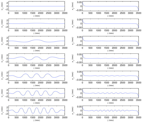
Figure 6: Numerical solutions for the local out-of-plane displacement $w_{1}$ (left) and local in-plane displacement $u_{1}$ (right) for the tip ($x=-b/2$) of the vulnerable flange. Individual solutions on equilibrium paths $C1$ to $C7$ are shown in sequence from top to bottom respectively.

illustrates the corresponding progression of the numerical solutions for the local buckling functions $w_{1}$ and $u_{1}$ from cell $C1$ to $C7$, where $C1$ represents the initial post-buckling equilibrium path generated from $\mathrm{C}$. Once a secondary bifurcation is triggered at $\mathrm{S}$, it is observed that the local buckling mode is contaminated by the global mode and interactive buckling ensues with the buckling deformation spreading towards the supports as new peaks and troughs are formed. Figure 7

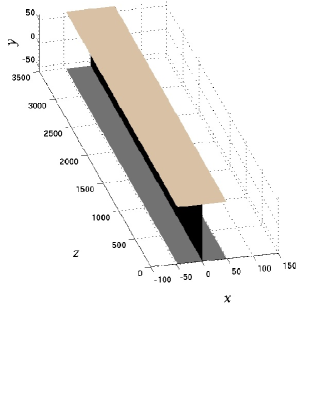
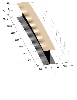
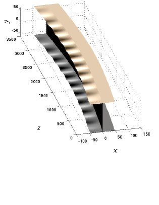
Figure 7: Numerical solutions of the system of equilibrium equations visualized on 3-dimensional representations of the strut. The results are shown for individual points on paths (a) $C1~{}(p=0.9039)$, (b) $C4~{}(p=0.9081)$, (c) $C7~{}(p=0.8111)$ and (d) $C10~{}(p=0.7177)$. All dimensions are in millimetres.

shows a selection of 3-dimensional representations of the deflected strut that comprise the components of global buckling ($W$ and $\theta$) and local buckling ($w_{i}$ and $u_{i}$) at a specific state on paths $C1$, $C4$, $C7$ and $C10$. As the equilibrium path develops to $C10$, the maximum out-of-plane displacement $w_{\mathrm{max}}$ approaches a value of $2.5~{}\mbox{$\mathrm{mm}$}$ which is roughly twice the flange thickness and can be regarded as large in terms of geometric assumptions. The interactive buckling pattern becomes effectively periodic on path $C10$. Any further deformation along the equilibrium path would be expected to cause restabilization to the system since the boundaries would begin to confine the spread of the buckling deformation. It should be stressed of course that any plastic deformation during the loading stage would destabilize the system significantly. Figure 8

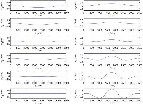
Figure 8: Numerical solutions for the local out-of-plane displacement $w_{2}$ (left) for the tip of the non-vulnerable flange ($x=b/2$) and $w_{1}$ (right) for the tip of the vulnerable flange ($x=-b/2$) for cells 1–3. Note the rapid decay of $w_{2}$ reflecting the reducing compression in that outstand once global buckling is triggered.

shows the comparison between the lateral displacement of the two flange outstands. The local buckling displacement in the non-vulnerable outstand $w_{2}$ decays to zero rapidly as the global mode amplitude increases during interactive buckling; by the third cell, $w_{2}$ has vanished implying that if global buckling occurs first, both $w_{2}$ and $u_{2}$ would be negligible.

The magnitude of direct and shear strains may be calculated once the governing differential equations are solved. The direct strain in the non-vulnerable part of the flange becomes tensile at $C10$ due to bending, whereas the maximum direct strain in the vulnerable part of the flange is approximately $1.3\times 10^{-3}(=0.13\%)$. This level of strain is confined to the ends of the strut and is also well below the yield strain of most structural steels; moreover for the stainless steels given in Becque and Rasmussen [4, 17], significant strain softening only begins from approximately $0.15\%$ strain and so quantitative comparisons can be made for the post-buckling response for the majority of the cells.

Systems that exhibit the phenomenon described above are termed in the literature to show “cellular buckling” [13] or “snaking” [14]. In such systems, progressive destabilization and restabilization is exhibited; currently, the destabilization is caused primarily by the interaction of the global and local instabilities, whereas the restabilization is caused by the stretching of the buckled plates when they bend into double curvature. As the amplitude of the global buckling mode $q_{s}$ increases, the compressive bending stress in the flange outstands increase also, which imply that progressively longer parts of the flange are susceptible to local buckling. Since local buckling is inherently stable, the drop in the load from the unstable mode interaction is limited due to the stretching of the plate when it buckles into progressively smaller wavelengths. Therefore, the cellular buckling occurs due to the complementary effects of the unstable mode interaction and stable local buckling.

3.2 Global buckling critical

The strut with properties given in Table 1 with length $L$ being $4.0~{}\mathrm{m}$ is now analysed; in this case, global Euler buckling occurs first. Figure 9

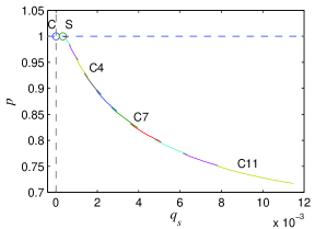
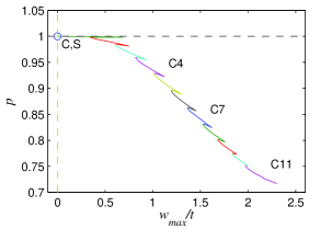
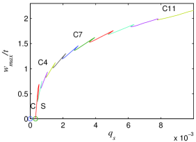
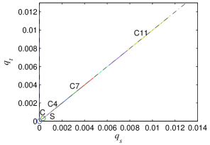
Figure 9: Numerical equilibrium paths for $L=4.0~{}\mathrm{m}$ where global buckling is critical. Graphs of the normalized force ratio $p$ versus (a) the generalized coordinate $q_{s}$ and (b) the maximum out-of-plane displacement of the buckled flange plate, in non-dimensional form $w_{\mathrm{max}}/t$, are shown. (c) shows $w_{\mathrm{max}}/t$ versus $q_{s}$ and (d) shows the relationship between the generalized coordinates $q_{s}$ and $q_{t}$ defining the global buckling mode during interactive buckling, with the dot-dash line showing the Euler–Bernoulli bending condition $q_{s}=q_{t}$.

shows plots of the equilibrium diagrams that correspond directly to Figure 5. This time, cellular buckling is triggered when the pure global mode is contaminated by the local mode. Since the global mode is only weakly stable, no significant post-buckling stiffness is exhibited initially. Moreover, since the global mode places the non-vulnerable flange outstand into less compression before any local buckling occurs, the functions $w_{2}$ and $u_{2}$ can be neglected as a consequence of the observations made in connection with Figure 8; this simplifies the formulation considerably.

The emergence of the buckling cells in sequence is very similar to that shown for the case where local buckling is critical and so it is not presented in detail for brevity. Nevertheless, with the model in place, quantitative comparisons can be made against existing experiments.

4 Validation and discussion

4.1 Comparison with experiments of Becque and Rasmussen

A recent experimental study of thin-walled I-section struts by Becque and Rasmussen [4, 17] focused on the case where local buckling is critical. Although the struts were made from a stainless steel alloy (ferritic AISI404), the compressive stress–strain curve showed that the material remained linearly elastic when the strain was below approximately $0.15\%$. Two specific tests were conducted on struts with material and geometric properties as given in Table 3.

Strut length $L$	$3.0~{}\mathrm{m}$	$2.5~{}\mathrm{m}$
Flange width $b$	$96.64~{}\mbox{$\mathrm{mm}$}$	$96.80~{}\mbox{$\mathrm{mm}$}$
Corner Radius $r$	$3.06~{}\mbox{$\mathrm{mm}$}$	$3.02~{}\mbox{$\mathrm{mm}$}$
Flange thickness $t$	$1.21~{}\mbox{$\mathrm{mm}$}$	$1.21~{}\mbox{$\mathrm{mm}$}$
Section depth $h$	$125.12~{}\mbox{$\mathrm{mm}$}$	$125.24~{}\mbox{$\mathrm{mm}$}$

Table 3: Geometric properties for the strut tests taken directly from [4, 17]. Recall that the thickness of the web $t_{w}=2t$. For both struts the initial Young’s modulus $E=195~{}\mathrm{kN/mm^{2}}$ and Poisson’s ratio $\nu=0.3$.

The initial out-of-straightness mid-length lateral deflections of the specimens of length $L$ being $3~{}\mathrm{m}$ and $2.5~{}\mathrm{m}$ were measured to be $L/3352$ and $L/16234$ respectively [17]. In order to make direct comparisons, numerical runs were conducted in Auto with the initial global buckling mode imperfection amplitude ratio $q_{s0}$ being equal to $3\times 10^{-4}$ and $6\times 10^{-5}$ respectively. The cross-section properties given in Table 3 were adapted slightly to consider the effective width of the flange, $b_{e}=b-2r$; the effective width was used in the numerics for the analytical model, the results of which follow.

The numerical continuation process was initiated from zero load with the process being illustrated in Figure 4(c). The value of $q_{s}$ was increased up to a bifurcation point, shown as $\mathrm{S}_{0}$ in Figure 4(c), after which interactive buckling was introduced. The equilibrium path then progressed to a limit point at which $P$ can be defined as the ultimate load $P_{U}$. Then destabilization and the cellular buckling behaviour was observed as described in the previous section. Figures 10

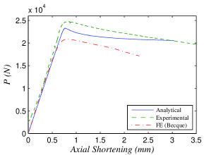
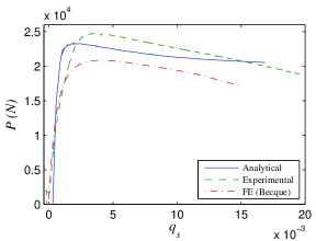
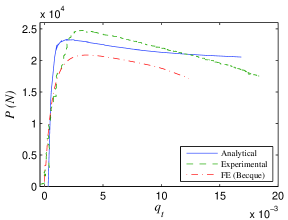
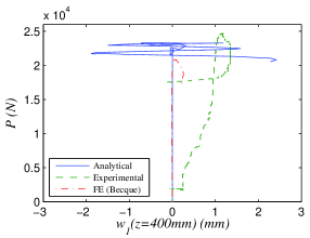
Figure 10: Numerical equilibrium paths comparing with Becque’s experiment with a strut of length $3~{}\mathrm{m}$. Graphs of the applied axial load $P$ versus (a) the total end shortening, (b) the generalized coordinate $q_{s}$, (c) the generalized coordinate $q_{t}$, (d) the out-of-plane displacement of the buckled flange plate $w_{1}$ measured at $z=400~{}\mbox{$\mathrm{mm}$}$ are shown. Solid lines show the current analytical model, whereas the dashed and dot-dashed lines respectively show the experimental and finite element results from [17].

and 11

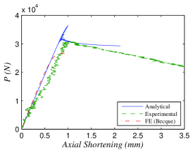
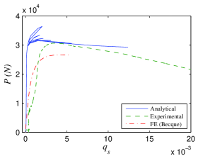
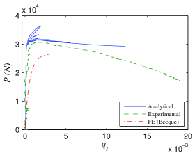
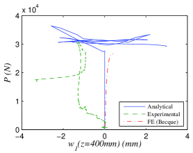
Figure 11: Numerical equilibrium paths comparing with Becque’s experiment with a strut of length $2.5~{}\mathrm{m}$. Graphs of the applied axial load $P$ versus (a) the total end shortening, (b) the generalized coordinate $q_{s}$, (c) the generalized coordinate $q_{t}$, (d) the out-of-plane displacement of the buckled flange plate $w_{1}$ measured at $z=400~{}\mbox{$\mathrm{mm}$}$ are shown. Solid lines show the current analytical model, whereas the dashed and dot-dashed lines respectively show the experimental and finite element results from [17].

show comparisons between the current analytical model, the experimental results from [4, 17] and the numerical models from [5, 17]. The comparisons show strong agreement between the analytical model and the results from the physical experiments, the correlation being clearly superior to the previous numerical results presented in [5, 17].

For the $3~{}\mathrm{m}$ length strut, the ultimate load was found to be $25.2~{}\mbox{$\mathrm{kN}$}$ from the experiment, which is approximately $3\%$ higher than the numerical value from the analytical model where $P_{U}=24.4~{}\mbox{$\mathrm{kN}$}$. It is also observed in Figure 10(d) that the theoretical local out-of-plane displacement $w_{1}$, at a location that was remote from the strut midspan ($z=400~{}\mbox{$\mathrm{mm}$}$), changes from positive to negative and vice versa several times. This is a signature of the cellular behaviour, indicating the progressive change in wavelength of the local buckling mode pattern. The actual experimental response, on the other hand, is always likely to jump to the final cell relatively rapidly once the initial instability is triggered. This was shown in the experiments conducted during work on the interactive buckling of beams [6], particularly in the cases where global and local buckling were triggered at similar load levels. The reason for this is that in a physical experiment, even with displacement control, the mechanical response in the region with snap-backs exhibits dynamic, rather than static, behaviour. Although in the current case the experiment did not pick up the full cellular response, it did show the change from positive to negative for $w_{1}$, which is a clear indication of the changing wavelength in the local buckling mode pattern. The interactive buckling wavelength $\Lambda$ can also be compared, which is defined in Figure 12.

Figure 12: Definition of local buckling wavelength $\Lambda$ from results for $w(\equiv w_{1})$ from the variational model.

The local buckling mode had a plate buckling wavelength that was measured to be $275~{}\mbox{$\mathrm{mm}$}$ with a modulated amplitude for this specific test [4]. The numerical results in the current work show that the value of $\Lambda$ is $280~{}\mbox{$\mathrm{mm}$}$ for the interactive buckling wavelength at the end of the equilibrium paths from the analytical model shown in Figure 10. The close comparison (less than $2\%$ difference) offers further grounds for encouragement for future developments of the current model.

For the $2.5~{}\mathrm{m}$ length strut, the features are similar; the ultimate load $P_{U}$ is $16\%$ higher than the maximum load shown in the experiment. However, this is only a very small part of the global picture. The graphs in Figure 11(a–c) show sequential snap-backs in the theoretical response almost immediately in the post-buckling range that reduce the true load-carrying capacity to levels which practically coincide with the experimental result, demonstrating an excellent overall comparison. In Figure 11(d), a similar response is observed to Figure 10(d). The change in sign of the out-of-plane displacement from the test clearly demonstrates the changing buckling wavelength again. Unfortunately, a numerical measurement of the plate buckling wavelength was not reported for this particular experiment.

Finally, it can be seen that the results from the analytical model and the experiments begin to diverge after a certain level of displacement. This is postulated to be as a result of material softening due to the use of stainless steel in the experiments, whereas linear elasticity is assumed throughout the analytical model. However, for the most part the close comparisons between the analytical model and the experimental results, in the authors’ opinion, validate the current modelling approach both qualitatively and quantitatively.

4.2 Future model enhancements

The success in capturing the interactive buckling behaviour allows for some speculation of how the current work may be extended. The technical difficulty of capturing sharp successive snap-back instabilities numerically most probably explains why the previous finite element models [5], although giving safe predictions for the global strength of the tested struts in [4, 17], showed a relatively indifferent comparison with the experiments. A possible way around this problem in future finite element modelling of such struts could be to introduce in turn a sequence of initial imperfections with different shapes that resemble the modes from each cell. This would allow an envelope of the nonlinear equilibrium solutions to be computed that resemble the actual post-buckling response.

Other issues that can be investigated are those regarding the assumption of the fixity between the elements of the cross-section, namely between the web and the flanges, and the introduction of lipped ends to the flanges. In terms of joint fixity, the flange–web junctions are modelled as pinned and hence are free to rotate. By modelling them as partially to fully rigid, a more extensive range of responses could be captured. With the resultant increase in structural stiffness in the cross-section this would introduce to the system, the local buckling load would definitely increase. However, the early evidence from a pilot study is that the post-buckling becomes less cellular as a result [21]. A similar effect may be obtained by attaching or designing flanges with lips to reduce the vulnerability to local buckling. However, lips introduce the possibility of distortional buckling [22] which, in this context, is known to resemble localized buckling [23, 24] rather than the cellular buckling found presently. Localization, in this context, can be more severely destabilizing than the cellular buckling. Work on this latter enhancement is currently in the early stages and hence the point regarding the potentially greater severity in the post-buckling instability is purely conjecture currently.

5 Concluding remarks

A nonlinear analytical model based on variational principles has been presented for axially-loaded thin-walled I-section struts buckling about the weak axis of bending. The model identifies an important and potentially dangerous interaction between global and local modes of instability, which leads to highly unstable cellular buckling through a series of snap-back instabilities. These result from the increasing contributions of buckling mode amplitudes forcing the flanges in more compression to buckle progressively. This process had also been observed in recent experimental work and in other components that suffer from a nonlinear interaction between global and local buckling. Comparisons with published experiments are excellent and validate the model. Extending the analytical approach would allow further study of the parameters that drive the behaviour and provide a greater and more profound understanding of the underlying phenomena. This, in turn, would provide designers with the information about the sensitivity of thin-walled components to small changes in geometry.

References

- Timoshenko and Gere [1961] Timoshenko, S.P., Gere, J.M.. Theory of elastic stability. New York, USA: McGraw-Hill; 1961.
- van der Neut [1969] van der Neut, A.. The interaction of local buckling and column failure of thin-walled compression members. In: Hetényi, M., Vincenti, W.G., editors. Proceedings of the 12th International Congress on Applied Mechanics. Berlin: Springer; 1969, p. 389–399.
- Hancock [1981] Hancock, G.J.. Interaction buckling in I-section columns. ASCE J Struct Eng 1981;107(1):165–179.
- Becque and Rasmussen [2009a] Becque, J., Rasmussen, K.J.R.. Experimental investigation of the interaction of local and overall buckling of stainless steel I-columns. ASCE J Struct Eng 2009a;135(11):1340–1348.
- Becque and Rasmussen [2009b] Becque, J., Rasmussen, K.J.R.. Numerical investigation of the interaction of local and overall buckling of stainless steel I-columns. ASCE J Struct Eng 2009b;135(11):1349–1356.
- Wadee and Gardner [2012] Wadee, M.A., Gardner, L.. Cellular buckling from mode interaction in I-beams under uniform bending. Proc R Soc A 2012;468:245–268.
- Hunt and Wadee [1998] Hunt, G.W., Wadee, M.A.. Localization and mode interaction in sandwich structures. Proc R Soc A 1998;454(1972):1197–1216.
- Wadee et al. [2010] Wadee, M.A., Yiatros, S., Theofanous, M.. Comparative studies of localized buckling in sandwich struts with different core bending models. Int J Non-Linear Mech 2010;45(2):111–120.
- Koiter and Pignataro [1976] Koiter, W.T., Pignataro, M.. A general theory for the interaction between local and overall buckling of stiffened panels. Tech. rept. WTHD 83; Delft University of Technology, Delft, The Netherlands; 1976.
- Pignataro et al. [2000] Pignataro, M., Pasca, M., Franchin, P.. Post-buckling analysis of corrugated panels in the presence of multiple interacting modes. Thin-Walled Struct 2000;36(1):47–66.
- Thompson and Hunt [1973] Thompson, J.M.T., Hunt, G.W.. A general theory of elastic stability. London: Wiley; 1973.
- Doedel and Oldeman [2009] Doedel, E.J., Oldeman, B.E.. Auto-07P: Continuation and bifurcation software for ordinary differential equations. Tech. Rep.; Department of Computer Science, Concordia University, Montreal, Canada; 2009. Available from http://indy.cs.concordia.ca/auto/.
- Hunt et al. [2000] Hunt, G.W., Peletier, M.A., Champneys, A.R., Woods, P.D., Wadee, M.A., Budd, C.J., et al. Cellular buckling in long structures. Nonlinear Dyn 2000;21(1):3–29.
- Burke and Knobloch [2007] Burke, J., Knobloch, E.. Homoclinic snaking: Structure and stability. Chaos 2007;17(3):037102.
- Hunt et al. [2003] Hunt, G.W., Lord, G.J., Peletier, M.A.. Cylindrical shell buckling: A characterization of localization and periodicity. Discrete Contin Dyn Syst-Ser B 2003;3(4):505–518.
- Wadee and Edmunds [2005] Wadee, M.A., Edmunds, R.. Kink band propagation in layered structures. J Mech Phys Solids 2005;53(9):2017–2035. doi:“bibinfo–doi˝–10.1016/j.jmps.2005.04.005˝.
- Becque [2008] Becque, J.. The interaction of local and overall buckling of cold-formed stainless steel columns. Ph.D. thesis; School of Civil Engineering, University of Sydney; Sydney, Australia; 2008.
- Bulson [1970] Bulson, P.S.. The stability of flat plates. London, UK: Chatto & Windus; 1970.
- Thompson and Hunt [1984] Thompson, J.M.T., Hunt, G.W.. Elastic instability phenomena. London: Wiley; 1984.
- Wadee [2000] Wadee, M.A.. Effects of periodic and localized imperfections on struts on nonlinear foundations and compression sandwich panels. Int J Solids Struct 2000;37(8):1191–1209. doi:“bibinfo–doi˝–10.1016/S0020-7683(98)00280-7˝.
- Wadee et al. [2013] Wadee, M.A., Bai, L., Camotim, D., Basaglia, C.. Behaviour of I-section columns experiencing local–overall mode interaction: Analytical and finite element modelling. In: Zingoni, A., editor. Proceedings of the 5th international conference on structural engineeering, mechanics and computation. 2013,In press.
- Schafer [2002] Schafer, B.W.. Local, distortional, and Euler buckling of thin-walled columns. ASCE J Struct Eng 2002;128(3):289–299.
- Hunt and Wadee [1991] Hunt, G.W., Wadee, M.K.. Comparative lagrangian formulations for localized buckling. Proc R Soc A 1991;434(1892):485–502.
- Wadee et al. [1997] Wadee, M.K., Hunt, G.W., Whiting, A.I.M.. Asymptotic and Rayleigh–Ritz routes to localized buckling solutions in an elastic instability problem. Proc R Soc A 1997;453(1965):2085–2107.