A Weak Galerkin Finite Element Method with Polynomial Reduction

Abstract

The novel idea of weak Galerkin (WG) finite element methods is on the use of weak functions and their weak derivatives defined as distributions. Weak functions and weak derivatives can be approximated by polynomials with various degrees. Different combination of polynomial spaces leads to different weak Galerkin finite element methods, which makes WG methods highly flexible and efficient in practical computation. This paper explores the possibility of optimal combination of polynomial spaces that minimize the number of unknowns in the numerical scheme, yet without compromising the accuracy of the numerical approximation. For illustrative purpose, the authors use second order elliptic problems to demonstrate the basic idea of polynomial reduction. A new weak Galerkin finite element method is proposed and analyzed. This new finite element scheme features piecewise polynomials of degree $k\geq 1$ on each element plus piecewise polynomials of degree $k-1\geq 0$ on the edge or face of each element. Error estimates of optimal order are established for the corresponding WG approximations in both a discrete $H^{1}$ norm and the standard $L^{2}$ norm. In addition, the paper presents a great deal of numerical experiments to demonstrate the power of the WG method in dealing with finite element partitions consisting of arbitrary polygons in two dimensional spaces or polyhedra in three dimensional spaces. The numerical examples include various finite element partitions such as triangular mesh, quadrilateral mesh, honey comb mesh in 2d and mesh with deformed cubes in 3d. The numerical results show a great promise of the robustness, reliability, flexibility and accuracy of the WG method.

1 Introduction

This paper is concerned with weak Galerkin (WG) finite element methods by exploring optimal use of polynomial approximating spaces. In general, weak Galerkin refers to finite element techniques for partial differential equations in which differential operators (e.g., gradient, divergence, curl, Laplacian) are approximated by weak forms as distributions. The main idea of weak Galerkin finite element methods is the use of weak functions and their corresponding discrete weak derivatives in algorithm design. For the second order elliptic equation, weak functions have the form of $v=\{v_{0},v_{b}\}$ with $v=v_{0}$ inside of each element and $v=v_{b}$ on the boundary of the element. Both $v_{0}$ and $v_{b}$ can be approximated by polynomials in $P_{\ell}(T)$ and $P_{s}(e)$ respectively, where $T$ stands for an element and $e$ the edge or face of $T$, $\ell$ and $s$ are non-negative integers with possibly different values. Weak derivatives are defined for weak functions in the sense of distributions. For computing purpose, one needs to approximate the weak derivatives by polynomials. For example, for the weak gradient operator, one may approximate it in the polynomial space $[P_{m}(T)]^{d}$. Various combination of $(P_{\ell}(T),P_{s}(e),[P_{m}(T)]^{d})$ leads to different class of weak Galerkin methods tailored for specific partial differential equations. The goal of this paper is to explore optimal combination of the polynomial spaces $P_{\ell}(T)$ and $P_{s}(e)$ that minimizes the number of unknowns without compromising the rate of convergence for the corresponding WG method.

For simplicity, we demonstrate the idea of optimality for polynomials by using the second order elliptic problem that seeks an unknown function $u$ satisfying

(1) $$-\nabla\cdot(a\nabla u) = f,\quad\mbox{in}\;\Omega,$$

(2) $$u = g,\quad\mbox{on}\;\partial\Omega,$$

where $\Omega$ is a polytopal domain in $\mathbb{R}^{d}$ (polygonal or polyhedral domain for $d=2,3$), $\nabla u$ denotes the gradient of the function $u$, and $a$ is a symmetric $d\times d$ matrix-valued function in $\Omega$. We shall assume that there exists a positive number $\lambda>0$ such that

(3) $$\xi^{t}a\xi\geq\lambda\xi^{t}\xi,\qquad\forall\xi\in\mathbb{R}^{d}.$$

Here $\xi$ is understood as a column vector and $\xi^{t}$ is the transpose of $\xi$.

A weak Galerkin method has been introduced and analyzed in [8] for second order elliptic equations based on a discrete weak gradient arising from local RT [7] or BDM [1] elements. More specifically, in the case of BDM element of order $k\geq 1$, the gradient space is taken as $[P_{m}(T)]^{d}\equiv[P_{k}(T)]^{d}$ and the weak functions are defined by using $(P_{\ell}(T),P_{s}(e))\equiv(P_{k-1}(T),P_{k}(e))$. For the RT element of $k\geq 0$, the gradient space is the usual RT element for the vector component while the weak functions are given by $(P_{\ell}(T),P_{s}(e))\equiv(P_{k}(T),P_{k}(e))$. Due to the use of the RT and BDM elements, the WG finite element formulation of [8] is limited to classical finite element partitions of triangles ($d=2$) or tetrahedra ($d=3$). In addition, the corresponding WG scheme exhibits a close connection with the standard mixed finite element method for (1)-(2).

The main goal of this paper is to investigate the possibility of optimal combination of polynomial spaces that minimize the number of unknowns in the numerical scheme without compromising the order of convergence. The new WG scheme will use the configuration of $(P_{k}(T),P_{k-1}(e),P_{k-1}(T)^{d})$, and the corresponding WG solution converges to the exact solution of (1)-(2) with rate of $O(h^{k})$ in $H^{1}$ and $O(h^{k+1})$ in $L^{2}$ norm, provided that the exact solution of the original problem is sufficiently smooth. It should be pointed out that the unknown $v_{0}$ associated with the interior of each element can be eliminated in terms of the unknown $v_{b}$ defined on the element boundary in practical implementation. This means that, for problems in $\mathbb{R}^{2}$, only edges of the finite element partition shall contribute unknowns ($k$ unknowns from each edge) to the global stiffness matrix problem. The new WG scheme is, therefore, a natural extension of the classical Crouzix-Raviart $P_{1}$ non-conforming triangular element to arbitrary order and arbitrary polygonal partitions.

It have been proved rigorously in [9] that $P_{k}$ type of polynomials can be used in weak Galerkin finite element procedures on any polygonal/polyhedral elements. It contrasts to the use of polynomials $P_{k}$ for triangular elements and tensor products $Q_{k}$ for quadrilateral elements in classic finite element methods. In practice, allowing arbitrary shape in finite element partition provides a great flexibility in both numerical approximation and mesh generation, especially in regions where the domain geometry is complex. Such a flexibility is also very much appreciated in adaptive mesh refinement methods. Another objective of this paper is to study the reliability, flexibility and accuracy of the weak Galerkin method through extensive numerical tests. The first and second order weak Galerkin elements are tested on partitions with different shape of polygons and polyhedra. Our numerical results show optimal order of convergence for $k=1,2$ on triangular, quadrilateral, honey comb meshes in 2d and deformed cube in 3d.

One close relative of the WG finite element method of this paper is the hybridizable discontinuous Galerkin (HDG) method [4]. But these two methods are fundamentally different in concept and formulation. The HDG method is formulated by using the standard mixed method approach for the usual system of first order equations, while the key to WG is the use of discrete weak differential operators. For the second order elliptic problem (1)-(2), these two methods share the same feature of approximating first order derivatives or fluxes through a formula that was commonly employed in the mixed finite element method. For high order PDEs, such as the biharmonic equation [6], the WG method is greatly different from the HDG. It should be emphasized that the concept of weak derivatives makes WG a widely applicable numerical technique for a large variety of partial differential equations which we shall report in forthcoming papers.

The paper is organized as follows. In Section 2, we shall review the definition of the weak gradient operator and its discrete analogues. In Section 3, we shall describe a new WG scheme. Section 4 will be devoted to a discussion of mass conservation for the WG scheme. In Section 5, we shall present some technical estimates for the usual $L^{2}$ projection operators. Section 6 is used to derive an optimal order error estimate for the WG approximation in both $H^{1}$ and $L^{2}$ norms. Finally in Section 7, we shall present some numerical results that confirm the theory developed in earlier sections.

2 Weak Gradient and Discrete Weak Gradient

Let $K$ be any polytopal domain with boundary $\partial K$. A weak function on the region $K$ refers to a function $v=\{v_{0},v_{b}\}$ such that $v_{0}\in L^{2}(K)$ and $v_{b}\in H^{\frac{1}{2}}(\partial K)$. The first component $v_{0}$ can be understood as the value of $v$ in $K$, and the second component $v_{b}$ represents $v$ on the boundary of $K$. Note that $v_{b}$ may not necessarily be related to the trace of $v_{0}$ on $\partial K$ should a trace be well-defined. Denote by $W(K)$ the space of weak functions on $K$; i.e.,

(4) $$W(K)=\{v=\{v_{0},v_{b}\}:\ v_{0}\in L^{2}(K),\;v_{b}\in H^{\frac{1}{2}}(\partial K)\}.$$

Define $(v,w)_{D}=\int_{D}vwdx$ and ${\langle}v,w{\rangle}_{\gamma}=\int_{\gamma}vwds$.

The weak gradient operator, as was introduced in [8], is defined as follows for the completion of the paper.

Definition 2.1.

The dual of $L^{2}(K)$ can be identified with itself by using the standard $L^{2}$ inner product as the action of linear functionals. With a similar interpretation, for any $v\in W(K)$, the weak gradient of $v$ is defined as a linear functional $\nabla_{w}v$ in the dual space of $H(div,K)$ whose action on each $q\in H(div,K)$ is given by

(5) $$(\nabla_{w}v,q)_{K}=-(v_{0},\nabla\cdot q)_{K}+\langle v_{b},q\cdot{\bf n}\rangle_{\partial K},$$

where ${\bf n}$ is the outward normal direction to $\partial K$, $(v_{0},\nabla\cdot q)_{K}=\int_{K}v_{0}(\nabla\cdot q)dK$ is the action of $v_{0}$ on $\nabla\cdot q$, and $\langle v_{b},q\cdot{\bf n}\rangle_{\partial K}$ is the action of $q\cdot{\bf n}$ on $v_{b}\in H^{\frac{1}{2}}(\partial K)$.

The Sobolev space $H^{1}(K)$ can be embedded into the space $W(K)$ by an inclusion map $i_{W}:\ H^{1}(K)\to W(K)$ defined as follows

$$i_{W}(\phi)=\{\phi|_{K},\phi|_{\partial K}\},\qquad\phi\in H^{1}(K).$$

With the help of the inclusion map $i_{W}$, the Sobolev space $H^{1}(K)$ can be viewed as a subspace of $W(K)$ by identifying each $\phi\in H^{1}(K)$ with $i_{W}(\phi)$. Analogously, a weak function $v=\{v_{0},v_{b}\}\in W(K)$ is said to be in $H^{1}(K)$ if it can be identified with a function $\phi\in H^{1}(K)$ through the above inclusion map. It is not hard to see that the weak gradient is identical with the strong gradient (i.e., $\nabla_{w}v=\nabla v$) for smooth functions $v\in H^{1}(K)$.

Denote by $P_{r}(K)$ the set of polynomials on $K$ with degree no more than $r$. We can define a discrete weak gradient operator by approximating $\nabla_{w}$ in a polynomial subspace of the dual of $H(div,K)$.

Definition 2.2.

The discrete weak gradient operator, denoted by $\nabla_{w,r,K}$, is defined as the unique polynomial $(\nabla_{w,r,K}v)\in[P_{r}(K)]^{d}$ satisfying the following equation

(6) $$(\nabla_{w,r,K}v,q)_{K}=-(v_{0},\nabla\cdot q)_{K}+\langle v_{b},q\cdot{\bf n}\rangle_{\partial K},\qquad\forall q\in[P_{r}(K)]^{d}.$$

By applying the usual integration by part to the first term on the right hand side of (6), we can rewrite the equation (6) as follows

(7) $$(\nabla_{w,r,K}v,q)_{K}=(\nabla v_{0},q)_{K}+\langle v_{b}-v_{0},q\cdot{\bf n}\rangle_{\partial K},\qquad\forall q\in[P_{r}(K)]^{d}.$$

3 Weak Galerkin Finite Element Schemes

Let ${\cal T}_{h}$ be a partition of the domain $\Omega$ consisting of polygons in two dimension or polyhedra in three dimension satisfying a set of conditions specified in [9]. Denote by ${\cal E}_{h}$ the set of all edges or flat faces in ${\cal T}_{h}$, and let ${\cal E}_{h}^{0}={\cal E}_{h}\backslash\partial\Omega$ be the set of all interior edges or flat faces. For every element $T\in{\mathcal{T}}_{h}$, we denote by $h_{T}$ its diameter and mesh size $h=\max_{T\in{\mathcal{T}}_{h}}h_{T}$ for ${\cal T}_{h}$.

For a given integer $k\geq 1$, let $V_{h}$ be the weak Galerkin finite element space associated with ${\mathcal{T}}_{h}$ defined as follows

(8) $$V_{h}=\{v=\{v_{0},v_{b}\}:\;v_{0}|_{T}\in P_{k}(T),\ v_{b}|_{e}\in P_{k-1}(e),\ e\in{\partial T},T\in{\mathcal{T}}_{h}\}$$

and

(9) $$V^{0}_{h}=\{v:\ v\in V_{h},\ v_{b}=0\mbox{ on }\partial\Omega\}.$$

We would like to emphasize that any function $v\in V_{h}$ has a single value $v_{b}$ on each edge $e\in{\mathcal{E}}_{h}$.

For each element $T\in{\mathcal{T}}_{h}$, denote by $Q_{0}$ the $L^{2}$ projection from $L^{2}(T)$ to $P_{k}(T)$ and by $Q_{b}$ the $L^{2}$ projection from $L^{2}(e)$ to $P_{k-1}(e)$. Denote by $\mathbb{Q}_{h}$ the $L^{2}$ projection onto the local discrete gradient space $[P_{k-1}(T)]^{d}$. Let $V=H^{1}(\Omega)$. We define a projection operator $Q_{h}:V\to V_{h}$ so that on each element $T\in{\mathcal{T}}_{h}$

(10) $$Q_{h}v=\{Q_{0}v_{0},Q_{b}v_{b}\},\qquad\{v_{0},v_{b}\}=i_{W}(v)\in W(T).$$

Denote by $\nabla_{w,k-1}$ the discrete weak gradient operator on the finite element space $V_{h}$ computed by using (6) on each element $T$; i.e.,

$$(\nabla_{w,k-1}v)|_{T}=\nabla_{w,k-1,T}(v|_{T}),\qquad\forall v\in V_{h}.$$

For simplicity of notation, from now on we shall drop the subscript $k-1$ in the notation $\nabla_{w,k-1}$ for the discrete weak gradient.

Now we introduce two forms on $V_{h}$ as follows:

$$a(v,w) = \sum_{T\in{\cal T}_{h}}(a\nabla_{w}v,\nabla_{w}w)_{T},$$

$$s(v,w) = \rho\sum_{T\in{\cal T}_{h}}h_{T}^{-1}\langle Q_{b}v_{0}-v_{b},Q_{b}w_{0}-w_{b}\rangle_{\partial T},$$

where $\rho$ can be any positive number. In practical computation, one might set $\rho=1$. Denote by $a_{s}(\cdot,\cdot)$ a stabilization of $a(\cdot,\cdot)$ given by

$$a_{s}(v,w)=a(v,w)+s(v,w).$$

Weak Galerkin Algorithm 1.

A numerical approximation for (1) and (2) can be obtained by seeking $u_{h}=\{u_{0},u_{b}\}\in V_{h}$ satisfying both $u_{b}=Q_{b}g$ on $\partial\Omega$ and the following equation:

(11) $$a_{s}(u_{h},v)=(f,v_{0}),\quad\forall\ v=\{v_{0},v_{b}\}\in V_{h}^{0}.$$

Note that the system (11) is symmetric and positive definite for any parameter value of $\rho>0$.

Next, we justify the well-postedness of the scheme (11). For any $v\in V_{h}$, let

(12) $${|||}v{|||}:=\sqrt{a_{s}(v,v)}.$$

It is not hard to see that ${|||}\cdot{|||}$ defines a semi-norm in the finite element space $V_{h}$. We claim that this semi-norm becomes to be a full norm in the finite element space $V_{h}^{0}$. It suffices to check the positivity property for ${|||}\cdot{|||}$. To this end, assume that $v\in V_{h}^{0}$ and ${|||}v{|||}=0$. It follows that

$$(a\nabla_{w}v,\nabla_{w}v)+\rho\sum_{T\in{\mathcal{T}}_{h}}h_{T}^{-1}\langle Q_{b}v_{0}-v_{b},Q_{b}v_{0}-v_{b}\rangle_{\partial T}=0,$$

which implies that $\nabla_{w}v=0$ on each element $T$ and $Q_{b}v_{0}=v_{b}$ on ${\partial T}$. It follows from $\nabla_{w}v=0$ and (7) that for any $q\in[P_{k-1}(T)]^{d}$

$$0 = (\nabla_{w}v,q)_{T}$$

$$= (\nabla v_{0},q)_{T}-\langle v_{0}-v_{b},q\cdot{\bf n}\rangle_{\partial T}$$

$$= (\nabla v_{0},q)_{T}-\langle Q_{b}v_{0}-v_{b},q\cdot{\bf n}\rangle_{\partial T}$$

$$= (\nabla v_{0},q)_{T}.$$

Letting $q=\nabla v_{0}$ in the equation above yields $\nabla v_{0}=0$ on $T\in{\cal T}_{h}$. Thus, $v_{0}=const$ on every $T\in{\mathcal{T}}_{h}$. This, together with the fact that $Q_{b}v_{0}=v_{b}$ on $\partial T$ and $v_{b}=0$ on $\partial\Omega$, implies that $v_{0}=v_{b}=0$.

Lemma 1.

The weak Galerkin finite element scheme (11) has a unique solution.

Proof.

If $u_{h}^{(1)}$ and $u_{h}^{(2)}$ are two solutions of (11), then $e_{h}=u_{h}^{(1)}-u_{h}^{(2)}$ would satisfy the following equation

$$a_{s}(e_{h},v)=0,\qquad\forall v\in V_{h}^{0}.$$

Note that $e_{h}\in V_{h}^{0}$. Then by letting $v=e_{h}$ in the above equation we arrive at

$${|||}e_{h}{|||}^{2}=a_{s}(e_{h},e_{h})=0.$$

It follows that $e_{h}\equiv 0$, or equivalently, $u_{h}^{(1)}\equiv u_{h}^{(2)}$. This completes the proof of the lemma. ∎

4 Mass Conservation

The second order elliptic equation (1) can be rewritten in a conservative form as follows:

$$\nabla\cdot q=f,\quad q=-a\nabla u.$$

Let $T$ be any control volume. Integrating the first equation over $T$ yields the following integral form of mass conservation:

(13) $$\int_{\partial T}q\cdot{\bf n}ds=\int_{T}fdT.$$

We claim that the numerical approximation from the weak Galerkin finite element method (11) for (1) retains the mass conservation property (13) with an appropriately defined numerical flux $q_{h}$. To this end, for any given $T\in{\cal T}_{h}$, we chose in (11) a test function $v=\{v_{0},v_{b}=0\}$ so that $v_{0}=1$ on $T$ and $v_{0}=0$ elsewhere. It follows from (11) that

(14) $$\int_{T}a\nabla_{w}u_{h}\cdot\nabla_{w}vdT+\rho h_{T}^{-1}\int_{\partial T}(Q_{b}u_{0}-u_{b})ds=\int_{T}fdT.$$

Let $\mathbb{Q}_{h}$ be the local $L^{2}$ projection onto the gradient space $[P_{k-1}(T)]^{d}$. Using the definition (6) for $\nabla_{w}v$ one arrives at

(15) $$\int_{T}a\nabla_{w}u_{h}\cdot\nabla_{w}vdT = \int_{T}\mathbb{Q}_{h}(a\nabla_{w}u_{h})\cdot\nabla_{w}vdT$$

$$= -\int_{T}\nabla\cdot\mathbb{Q}_{h}(a\nabla_{w}u_{h})dT$$

$$= -\int_{\partial T}\mathbb{Q}_{h}(a\nabla_{w}u_{h})\cdot{\bf n}ds.$$

Substituting (15) into (14) yields

(16) $$\int_{\partial T}\left\{-\mathbb{Q}_{h}\left(a\nabla_{w}u_{h}\right)+\rho h_{T}^{-1}(Q_{b}u_{0}-u_{b}){\bf n}\right\}\cdot{\bf n}ds=\int_{T}fdT,$$

which indicates that the weak Galerkin method conserves mass with a numerical flux given by

$$q_{h}=-\mathbb{Q}_{h}\left(a\nabla_{w}u_{h}\right)+\rho h_{T}^{-1}(Q_{b}u_{0}-u_{b}){\bf n}.$$

Next, we verify that the normal component of the numerical flux, namely $q_{h}\cdot{\bf n}$, is continuous across the edge of each element $T$. To this end, let $e$ be an interior edge/face shared by two elements $T_{1}$ and $T_{2}$. Choose a test function $v=\{v_{0},v_{b}\}$ so that $v_{0}\equiv 0$ and $v_{b}=0$ everywhere except on $e$. It follows from (11) that

$$\int_{T_{1}\cup T_{2}}a\nabla_{w}u_{h}\cdot\nabla_{w}vdT -\rho h_{T_{1}}^{-1}\int_{\partial T_{1}\cap e}(Q_{b}u_{0}-u_{b})|_{T_{1}}v_{b}ds$$

$$-\rho h_{T_{2}}^{-1}\int_{\partial T_{2}\cap e}(Q_{b}u_{0}-u_{b})|_{T_{2}}v_{b}ds$$

$$=0.$$

Using the definition of weak gradient (6) we obtain

$$\int_{T_{1}\cup T_{2}}a\nabla_{w}u_{h}\cdot\nabla_{w}vdT = \int_{T_{1}\cup T_{2}}\mathbb{Q}_{h}(a\nabla_{w}u_{h})\cdot\nabla_{w}vdT$$

$$= \int_{e}\left(\mathbb{Q}_{h}(a\nabla_{w}u_{h})|_{T_{1}}\cdot{\bf n}_{1}+\mathbb{Q}_{h}(a\nabla_{w}u_{h})|_{T_{2}}\cdot{\bf n}_{2}\right)v_{b}ds,$$

where ${\bf n}_{i}$ is the outward normal direction of $T_{i}$ on the edge $e$. Note that ${\bf n}_{1}+{\bf n}_{2}=0$. Substituting the above equation into (4) yields

$$\int_{e}\left(-\mathbb{Q}_{h}(a\nabla_{w}u_{h})|_{T_{1}}+\rho h_{T_{1}}^{-1}(Q_{b}u_{0}-u_{b})|_{T_{1}}{\bf n}_{1}\right)\cdot{\bf n}_{1}v_{b}ds$$

$$=-\int_{e}\left(-\mathbb{Q}_{h}(a\nabla_{w}u_{h})|_{T_{2}}+\rho h_{T_{2}}^{-1}(Q_{b}u_{0}-u_{b})|_{T_{2}}{\bf n}_{2}\right)\cdot{\bf n}_{2}v_{b}ds,$$

which shows the continuity of the numerical flux $q_{h}$ in the normal direction.

5 Some Technical Estimates

This section shall present some technical results useful for the forthcoming error analysis. The first one is a trace inequality established in [9] for functions on general shape regular partitions. More precisely, let $T$ be an element with $e$ as an edge. For any function $\varphi\in H^{1}(T)$, the following trace inequality holds true (see [9] for details):

(18) $$\|\varphi\|_{e}^{2}\leq C\left(h_{T}^{-1}\|\varphi\|_{T}^{2}+h_{T}\|\nabla\varphi\|_{T}^{2}\right).$$

Another useful result is a commutativity property for some projection operators.

Lemma 2.

Let $Q_{h}$ and $\mathbb{Q}_{h}$ be the $L^{2}$ projection operators defined in previous sections. Then, on each element $T\in{\mathcal{T}}_{h}$, we have the following commutative property

(19) $$\nabla_{w}(Q_{h}\phi)=\mathbb{Q}_{h}(\nabla\phi),\quad\forall\phi\in H^{1}(T).$$

Proof.

Using (6), the integration by parts and the definitions of $Q_{h}$ and $\mathbb{Q}_{h}$, we have that for any $\tau\in[P_{k-1}(T)]^{d}$

$$(\nabla_{w}(Q_{h}\phi),\tau)_{T} = -(Q_{0}\phi,\nabla\cdot\tau)_{T}+\langle Q_{b}\phi,\tau\cdot{\bf n}\rangle_{{\partial T}}$$

$$= -(\phi,\nabla\cdot\tau)_{T}+\langle\phi,\tau\cdot{\bf n}\rangle_{\partial T}$$

$$= (\nabla\phi,\tau)_{T}$$

$$= (\mathbb{Q}_{h}(\nabla\phi),\tau)_{T},$$

which implies the desired identity (19). ∎

The following lemma provides some estimates for the projection operators $Q_{h}$ and $\mathbb{Q}_{h}$. Observe that the underlying mesh ${\mathcal{T}}_{h}$ is assumed to be sufficiently general to allow polygons or polyhedra. A proof of the lemma can be found in [9]. It should be pointed out that the proof of the lemma requires some non-trivial technical tools in analysis, which have also been established in [9].

Lemma 3.

Let ${\mathcal{T}}_{h}$ be a finite element partition of $\Omega$ that is shape regular. Then, for any $\phi\in H^{k+1}(\Omega)$, we have

(20) $$\sum_{T\in{\mathcal{T}}_{h}}\|\phi-Q_{0}\phi\|_{T}^{2}+\sum_{T\in{\mathcal{T}}_{h}}h_{T}^{2}\|\nabla(\phi-Q_{0}\phi)\|_{T}^{2}\leq Ch^{2(k+1)}\|\phi\|^{2}_{k+1},$$

(21) $$\sum_{T\in{\mathcal{T}}_{h}}\|a(\nabla\phi-\mathbb{Q}_{h}(\nabla\phi))\|^{2}_{T}\leq Ch^{2k}\|\phi\|^{2}_{k+1}.$$

Here and in what follows of this paper, $C$ denotes a generic constant independent of the meshsize $h$ and the functions in the estimates.

In the finite element space $V_{h}$, we introduce a discrete $H^{1}$ semi-norm as follows:

(22) $$\|v\|_{1,h}=\left(\sum_{T\in{\mathcal{T}}_{h}}\left(\|\nabla v_{0}\|_{T}^{2}+h_{T}^{-1}\|Q_{b}v_{0}-v_{b}\|_{\partial T}\right)\right)^{\frac{1}{2}}.$$

The following lemma indicates that $\|\cdot\|_{1,h}$ is equivalent to the trip-bar norm (12).

Lemma 4.

There exist two positive constants $C_{1}$ and $C_{2}$ such that for any $v=\{v_{0},v_{b}\}\in V_{h}$, we have

(23) $$C_{1}\|v\|_{1,h}\leq{|||}v{|||}\leq C_{2}\|v\|_{1,h}.$$

Proof.

For any $v=\{v_{0},v_{b}\}\in V_{h}$, it follows from the definition of weak gradient (7) and $Q_{b}$ that

(24) $$(\nabla_{w}v,q)_{T}=(\nabla v_{0},q)_{T}+{\langle}v_{b}-Q_{b}v_{0},q\cdot{\bf n}{\rangle}_{\partial T},\quad\forall q\in[P_{k-1}(T)]^{d}.$$

By letting $q=\nabla_{w}v$ in (24) we arrive at

$$(\nabla_{w}v,\nabla_{w}v)_{T}=(\nabla v_{0},\nabla_{w}v)_{T}+{\langle}v_{b}-Q_{b}v_{0},\nabla_{w}v\cdot{\bf n}{\rangle}_{\partial T}.$$

From the trace inequality (18) and the inverse inequality we have

$$(\nabla_{w}v,\nabla_{w}v)_{T} \leq \|\nabla v_{0}\|_{T}\|\nabla_{w}v\|_{T}+\|Q_{b}v_{0}-v_{b}\|_{\partial T}\|\nabla_{w}v\|_{\partial T}$$

$$\leq \|\nabla v_{0}\|_{T}\|\nabla_{w}v\|_{T}+Ch_{T}^{-1/2}\|Q_{b}v_{0}-v_{b}\|_{\partial T}\|\nabla_{w}v\|_{T}$$

Thus,

$$\|\nabla_{w}v\|_{T}\leq C\left(\|\nabla v_{0}\|_{T}^{2}+h_{T}^{-1}\|Q_{b}v_{0}-v_{b}\|_{\partial T}^{2}\right)^{\frac{1}{2}},$$

which verifies the upper bound of ${|||}v{|||}$. As to the lower bound, we chose $q=\nabla v_{0}$ in (24) to obtain

$$(\nabla_{w}v,\nabla v_{0})_{T}=(\nabla v_{0},\nabla v_{0})_{T}+{\langle}v_{b}-Q_{b}v_{0},\nabla v_{0}\cdot{\bf n}{\rangle}_{\partial T}.$$

Thus, from the trace an inverse inequality we have

$$\|\nabla v_{0}\|_{T}^{2}\leq\|\nabla_{w}v\|_{T}\|\nabla v_{0}\|_{T}+Ch_{T}^{-1/2}\|Q_{b}v_{0}-v_{b}\|_{\partial T}\|\nabla v_{0}\|_{T}.$$

This leads to

$$\|\nabla v_{0}\|_{T}\leq C\left(\|\nabla_{w}v\|_{T}^{2}+Ch_{T}^{-1}\|Q_{b}v_{0}-v_{b}\|_{\partial T}^{2}\right)^{\frac{1}{2}},$$

which verifies the lower bound for ${|||}v{|||}$. Collectively, they complete the proof of the lemma. ∎

Lemma 5.

Assume that ${\mathcal{T}}_{h}$ is shape regular. Then for any $w\in H^{k+1}(\Omega)$ and $v=\{v_{0},v_{b}\}\in V_{h}$, we have

(25) $$|s(Q_{h}w,v)| \leq Ch^{k}\|w\|_{k+1}{|||}v{|||},$$

(26) $$\left|\ell_{w}(v)\right| \leq Ch^{k}\|w\|_{k+1}{|||}v{|||},$$

where $\ell_{w}(v)=\sum_{T\in{\mathcal{T}}_{h}}\langle a(\nabla w-\mathbb{Q}_{h}\nabla w)\cdot{\bf n},\;v_{0}-v_{b}\rangle_{\partial T}$.

Proof.

Using the definition of $Q_{b}$, (18), and (20), we obtain

$$|s(Q_{h}w,v)| = \left|\sum_{T\in{\mathcal{T}}_{h}}h_{T}^{-1}\langle Q_{b}(Q_{0}w)-Q_{b}w,\;Q_{b}v_{0}-v_{b}\rangle_{\partial T}\right|$$

$$= \left|\sum_{T\in{\mathcal{T}}_{h}}h_{T}^{-1}\langle Q_{0}w-w,\;Q_{b}v_{0}-v_{b}\rangle_{\partial T}\right|$$

$$\leq C\left(\sum_{T\in{\mathcal{T}}_{h}}(h_{T}^{-2}\|Q_{0}w-w\|_{T}^{2}+\|\nabla(Q_{0}w-w)\|_{T}^{2})\right)^{\frac{1}{2}}\cdot$$

$$\left(\sum_{T\in{\mathcal{T}}_{h}}h_{T}^{-1}\|Q_{b}v_{0}-v_{b}\|^{2}_{{\partial T}}\right)^{\frac{1}{2}}$$

$$\leq Ch^{k}\|w\|_{k+1}{|||}v{|||}.$$

As to (26), it follows from the Cauchy-Schwarz inequality, the trace inequality (18) and the estimate (21) that

$$|\ell_{w}(v)| = \left|\sum_{T\in{\mathcal{T}}_{h}}\langle a(\nabla w-\mathbb{Q}_{h}\nabla w)\cdot{\bf n},v_{0}-v_{b}\rangle_{\partial T}\right|$$

$$\leq C\sum_{T\in{\mathcal{T}}_{h}}\|a(\nabla w-\mathbb{Q}_{h}\nabla w)\|_{{\partial T}}\|v_{0}-v_{b}\|_{\partial T}$$

$$\leq C\left(\sum_{T\in{\mathcal{T}}_{h}}h_{T}\|a(\nabla w-\mathbb{Q}_{h}\nabla w)\|_{{\partial T}}^{2}\right)^{\frac{1}{2}}\left(\sum_{T\in{\mathcal{T}}_{h}}h_{T}^{-1}\|v_{0}-v_{b}\|_{\partial T}^{2}\right)^{\frac{1}{2}}$$

$$\leq Ch^{k}\|w\|_{k+1}\left(\sum_{T\in{\mathcal{T}}_{h}}h_{T}^{-1}\|v_{0}-v_{b}\|_{\partial T}^{2}\right)^{\frac{1}{2}}.$$

Using the trace inequality (18) and the approximation property of the $L^{2}$ projection operator we obtain

$$\|v_{0}-v_{b}\|_{\partial T} \leq \|v_{0}-Q_{b}v_{0}\|_{\partial T}+\|Q_{b}v_{0}-v_{b}\|_{\partial T}$$

$$\leq Ch_{T}^{1/2}\|\nabla v_{0}\|_{T}+\|Q_{b}v_{0}-v_{b}\|_{\partial T}.$$

Substituting the above inequality into (5) yields

(28) $$|\ell_{w}(v)|\leq Ch^{k}\|w\|_{k+1}\left(\sum_{T\in{\mathcal{T}}_{h}}\left\{\|\nabla v_{0}\|_{T}^{2}+h_{T}^{-1}\|Q_{b}v_{0}-v_{b}\|_{\partial T}^{2}\right\}\right)^{\frac{1}{2}},$$

which, along with the estimate (23), verifies the desired estimate (26). ∎

6 Error Analysis

The goal of this section is to establish some error estimates for the weak Galerkin finite element solution $u_{h}$ arising from (11). The error will be measured in two natural norms: the triple-bar norm as defined in (12) and the standard $L^{2}$ norm. The triple bar norm is essentially a discrete $H^{1}$ norm for the underlying weak function.

For simplicity of analysis, we assume that the coefficient tensor $a$ in (1) is a piecewise constant matrix with respect to the finite element partition ${\mathcal{T}}_{h}$. The result can be extended to variable tensors without any difficulty, provided that the tensor $a$ is piecewise sufficiently smooth.

6.1 Error equation

Let $u_{h}=\{u_{0},u_{b}\}\in V_{h}$ be the weak Galerkin finite element solution arising from the numerical scheme (11). Assume that the exact solution of (1)-(2) is given by $u$. The $L^{2}$ projection of $u$ in the finite element space $V_{h}$ is given by

$$Q_{h}u=\{Q_{0}u,Q_{b}u\}.$$

Let

$$e_{h}=\{e_{0},e_{b}\}=\{Q_{0}u-u_{0},Q_{b}u-u_{b}\}$$

be the error between the WG finite element solution and the $L^{2}$ projection of the exact solution.

Lemma 6.

Let $e_{h}$ be the error of the weak Galerkin finite element solution arising from (11). Then, for any $v\in V_{h}^{0}$ we have

(29) $$a_{s}(e_{h},v)=\ell_{u}(v)+s(Q_{h}u,v),$$

where $\ell_{u}(v)=\sum_{T\in{\mathcal{T}}_{h}}\langle a(\nabla u-\mathbb{Q}_{h}\nabla u)\cdot{\bf n},v_{0}-v_{b}\rangle_{\partial T}$.

Proof.

Testing (1) by using $v_{0}$ of $v=\{v_{0},v_{b}\}\in V_{h}^{0}$ we arrive at

(30) $$\sum_{T\in{\mathcal{T}}_{h}}(a\nabla u,\nabla v_{0})_{T}-\sum_{T\in{\mathcal{T}}_{h}}\langle a\nabla u\cdot{\bf n},v_{0}-v_{b}\rangle_{\partial T}=(f,v_{0}),$$

where we have used the fact that $\sum_{T\in{\mathcal{T}}_{h}}\langle a\nabla u\cdot{\bf n},v_{b}\rangle_{\partial T}=0$. To deal with the term $\sum_{T\in{\mathcal{T}}_{h}}(a\nabla u,\nabla v_{0})_{T}$ in (30), we need the following equation. For any $\phi\in H^{1}(T)$ and $v\in V_{h}$, it follows from (19), the definition of the discrete weak gradient (6), and the integration by parts that

(31) $$(a\nabla_{w}Q_{h}\phi,\nabla_{w}v)_{T} = (a\mathbb{Q}_{h}(\nabla\phi),\nabla_{w}v)_{T}$$

$$= -(v_{0},\nabla\cdot(a\mathbb{Q}_{h}\nabla\phi))_{T}+\langle v_{b},(a\mathbb{Q}_{h}\nabla\phi)\cdot{\bf n}\rangle_{\partial T}$$

$$= (\nabla v_{0},a\mathbb{Q}_{h}\nabla\phi)_{T}-\langle v_{0}-v_{b},(a\mathbb{Q}_{h}\nabla\phi)\cdot{\bf n}\rangle_{\partial T}$$

$$= (a\nabla\phi,\nabla v_{0})_{T}-{\langle}(a\mathbb{Q}_{h}\nabla\phi)\cdot{\bf n},\ v_{0}-v_{b}{\rangle}_{\partial T}.$$

By letting $\phi=u$ in (31), we have from combining (31) and (30) that

$$\sum_{T\in{\mathcal{T}}_{h}}(a\nabla_{w}Q_{h}u,\nabla_{w}v)_{T} = (f,v_{0})+\sum_{T\in{\mathcal{T}}_{h}}\langle a(\nabla u-\mathbb{Q}_{h}\nabla u)\cdot{\bf n},v_{0}-v_{b}\rangle_{\partial T}$$

$$= (f,v_{0})+\ell_{u}(v).$$

Adding $s(Q_{h}u,v)$ to both sides of the above equation gives

(32) $$a_{s}(Q_{h}u,v)=(f,v_{0})+\ell_{u}(v)+s(Q_{h}u,v).$$

Subtracting (11) from (32) yields the following error equation,

$$a_{s}(e_{h},v)=\ell_{u}(v)+s(Q_{h}u,v),\quad\forall v\in V_{h}^{0}.$$

This completes the proof of the lemma. ∎

6.2 Error estimates

The error equation (29) can be used to derive the following error estimate for the WG finite element solution.

Theorem 7.

Let $u_{h}\in V_{h}$ be the weak Galerkin finite element solution of the problem (1)-(2) arising from (11). Assume the exact solution $u\in H^{k+1}(\Omega)$. Then, there exists a constant $C$ such that

(33) $${|||}u_{h}-Q_{h}u{|||}\leq Ch^{k}\|u\|_{k+1}.$$

Proof.

By letting $v=e_{h}$ in (29), we have

(34) $${|||}e_{h}{|||}^{2} = \ell_{u}(e_{h})+s(Q_{h}u,\;\ e_{h}).$$

It then follows from (25) and (26) that

$${|||}e_{h}{|||}^{2}\leq Ch^{k}\|u\|_{k+1}{|||}e_{h}{|||},$$

which implies (33). This completes the proof. ∎

Next, we will measure the difference between $u$ and $u_{h}$ in the discrete $H^{1}$ semi-norm $\|\cdot\|_{1,h}$ as defined in (22). Note that (22) can be easily extended to functions in $H^{1}(\Omega)+V_{h}$ through the inclusion map $i_{W}$.

Corollary 8.

Let $u_{h}\in V_{h}$ be the weak Galerkin finite element solution of the problem (1)-(2) arising from (11). Assume the exact solution $u\in H^{k+1}(\Omega)$. Then, there exists a constant $C$ such that

(35) $$\|u-u_{h}\|_{1,h}\leq Ch^{k}\|u\|_{k+1}.$$

Proof.

It follows from (23) and (33) that

$$\|Q_{h}u-u_{h}\|_{1,h}\leq C{|||}Q_{h}u-u_{h}{|||}\leq Ch^{k}\|u\|_{k+1}.$$

Using the triangle inequality, (20) and the equation above, we have

$$\|u-u_{h}\|_{1,h}\leq\|u-Q_{h}u\|_{1,h}+\|Q_{h}u-u_{h}\|_{1,h}\leq Ch^{k}\|u\|_{k+1}.$$

This completes the proof. ∎

In the rest of the section, we shall derive an optimal order error estimate for the weak Galerkin finite element scheme (11) in the usual $L^{2}$ norm by using a duality argument as was commonly employed in the standard Galerkin finite element methods [3, 2]. To this end, we consider a dual problem that seeks $\Phi\in H_{0}^{1}(\Omega)$ satisfying

(36) $$-\nabla\cdot(a\nabla\Phi) = e_{0}\quad\mbox{in}\;\Omega.$$

Assume that the above dual problem has the usual $H^{2}$-regularity. This means that there exists a constant $C$ such that

(37) $$\|\Phi\|_{2}\leq C\|e_{0}\|.$$

Theorem 9.

Let $u_{h}\in V_{h}$ be the weak Galerkin finite element solution of the problem (1)-(2) arising from (11). Assume the exact solution $u\in H^{k+1}(\Omega)$. In addition, assume that the dual problem (36) has the usual $H^{2}$-regularity. Then, there exists a constant $C$ such that

(38) $$\|u-u_{0}\|\leq Ch^{k+1}\|u\|_{k+1}.$$

Proof.

By testing (36) with $e_{0}$ we obtain

(39) $$\|e_{0}\|^{2} = -(\nabla\cdot(a\nabla\Phi),e_{0})$$

$$= \sum_{T\in{\mathcal{T}}_{h}}(a\nabla\Phi,\ \nabla e_{0})_{T}-\sum_{T\in{\mathcal{T}}_{h}}{\langle}a\nabla\Phi\cdot{\bf n},\ e_{0}-e_{b}{\rangle}_{{\partial T}},$$

where we have used the fact that $e_{b}=0$ on $\partial\Omega$. Setting $\phi=\Phi$ and $v=e_{h}$ in (31) yields

(40) $$(a\nabla_{w}Q_{h}\Phi,\;\nabla_{w}e_{h})_{T}=(a\nabla\Phi,\;\nabla e_{0})_{T}-{\langle}(a\mathbb{Q}_{h}\nabla\Phi)\cdot{\bf n},\ e_{0}-e_{b}{\rangle}_{\partial T}.$$

Substituting (40) into (39) gives

(41) $$\|e_{0}\|^{2} = (a\nabla_{w}e_{h},\ \nabla_{w}Q_{h}\Phi)+\sum_{T\in{\mathcal{T}}_{h}}{\langle}a(\mathbb{Q}_{h}\nabla\Phi-\nabla\Phi)\cdot{\bf n},\ e_{0}-e_{b}{\rangle}_{{\partial T}}$$

$$= (a\nabla_{w}e_{h},\ \nabla_{w}Q_{h}\Phi)+\ell_{\Phi}(e_{h}).$$

It follows from the error equation (29) that

(42) $$(a\nabla_{w}e_{h},\ \nabla_{w}Q_{h}\Phi) = \ell_{u}(Q_{h}\Phi)+s(Q_{h}u,\ Q_{h}\Phi)-s(e_{h},\ Q_{h}\Phi).$$

By combining (41) with (42) we arrive at

(43) $$\|e_{0}\|^{2}=\ell_{u}(Q_{h}\Phi)+s(Q_{h}u,\ Q_{h}\Phi)-s(e_{h},\ Q_{h}\Phi)+\ell_{\Phi}(e_{h}).$$

Let us bound the terms on the right hand side of (43) one by one. Using the triangle inequality, we obtain

(44) $$|\ell_{u}(Q_{h}\Phi)| = \left|\sum_{T\in{\mathcal{T}}_{h}}\langle a(\nabla u-\mathbb{Q}_{h}\nabla u)\cdot{\bf n},\;Q_{0}\Phi-Q_{b}\Phi\rangle_{\partial T}\right|$$

$$\leq \left|\sum_{T\in{\mathcal{T}}_{h}}\langle a(\nabla u-\mathbb{Q}_{h}\nabla u)\cdot{\bf n},\;Q_{0}\Phi-\Phi\rangle_{\partial T}\right|$$

$$+ \left|\sum_{T\in{\mathcal{T}}_{h}}\langle a(\nabla u-\mathbb{Q}_{h}\nabla u)\cdot{\bf n},\;\Phi-Q_{b}\Phi\rangle_{\partial T}\right|.$$

We first use the definition of $Q_{b}$ and the fact that $\Phi=0$ on $\partial\Omega$ to obtain

(45) $$\sum_{T\in{\mathcal{T}}_{h}}{\langle}a(\nabla u-\mathbb{Q}_{h}\nabla u)\cdot{\bf n},\Phi-Q_{b}\Phi{\rangle}_{\partial T}=\sum_{T\in{\mathcal{T}}_{h}}{\langle}a\nabla u\cdot{\bf n},\Phi-Q_{b}\Phi{\rangle}_{\partial T}=0.$$

From the trace inequality (18) and the estimate (20) we have

$$\left(\sum_{T\in{\mathcal{T}}_{h}}\|Q_{0}\Phi-\Phi\|^{2}_{\partial T}\right)^{1/2}\leq Ch^{\frac{3}{2}}\|\Phi\|_{2}$$

and

$$\left(\sum_{T\in{\mathcal{T}}_{h}}\|a(\nabla u-\mathbb{Q}_{h}\nabla u)\|^{2}_{\partial T}\right)^{1/2}\leq Ch^{k-\frac{1}{2}}\|u\|_{k+1}.$$

Thus, it follows from the Cauchy-Schwarz inequality and the above two estimates that

$$\left|\sum_{T\in{\mathcal{T}}_{h}}\langle a(\nabla u-\mathbb{Q}_{h}\nabla u)\cdot{\bf n},\;Q_{0}\Phi-\Phi\rangle_{\partial T}\right|$$

$$\leq C\left(\sum_{T\in{\mathcal{T}}_{h}}\|a(\nabla u-\mathbb{Q}_{h}\nabla u)\|^{2}_{\partial T}\right)^{1/2}\left(\sum_{T\in{\mathcal{T}}_{h}}\|Q_{0}\Phi-\Phi\|^{2}_{\partial T}\right)^{1/2}$$

(46) $$\leq Ch^{k+1}\|u\|_{k+1}\|\Phi\|_{2}.$$

Combining (44) with (45) and (46) yields

(47) $$|\ell_{u}(Q_{h}\Phi)|\leq Ch^{k+1}\|u\|_{k+1}\|\Phi\|_{2}.$$

Analogously, it follows from the definition of $Q_{b}$, the trace inequality (18), and the estimate (20) that

(48) $$\left|s(Q_{h}u,\;Q_{h}\Phi)\right| \leq \rho\sum_{T\in{\mathcal{T}}_{h}}h_{T}^{-1}\left|(Q_{b}(Q_{0}u)-Q_{b}u,\ Q_{b}(Q_{0}\Phi)-Q_{b}\Phi)_{\partial T}\right|$$

$$\leq \rho\sum_{T\in{\mathcal{T}}_{h}}h_{T}^{-1}\|Q_{b}(Q_{0}u-u)\|_{\partial T}\|Q_{b}(Q_{0}\Phi-\Phi)\|_{\partial T}$$

$$\leq \rho\sum_{T\in{\mathcal{T}}_{h}}h_{T}^{-1}\|Q_{0}u-u\|_{\partial T}\|Q_{0}\Phi-\Phi\|_{\partial T}$$

$$\leq C\left(\sum_{T\in{\mathcal{T}}_{h}}h_{T}^{-1}\|Q_{0}u-u\|^{2}_{\partial T}\right)^{1/2}\left(\sum_{T\in{\mathcal{T}}_{h}}h_{T}^{-1}\|Q_{0}\Phi-\Phi\|^{2}_{\partial T}\right)^{1/2}$$

$$\leq Ch^{k+1}\|u\|_{k+1}\|\Phi\|_{2}.$$

The estimates (25) with $k=1$ and the error estimate (33) imply

(49) $$|s(e_{h},\ Q_{h}\Phi)|\leq Ch\|\Phi\|_{2}{|||}e_{h}{|||}\leq Ch^{k+1}\|u\|_{k+1}\|\Phi\|_{2}.$$

Similarly, it follows from (26) and (33) that

(50) $$|\ell_{\Phi}(e_{h})| \leq Ch^{k+1}\|u\|_{k+1}\|\Phi\|_{2}.$$

Now substituting (47)-(50) into (43) yields

$$\|e_{0}\|^{2}\leq Ch^{k+1}\|u\|_{k+1}\|\Phi\|_{2},$$

which, combined with the regularity assumption (37) and the triangle inequality, gives the desired optimal order error estimate (38). ∎

7 Numerical Examples

In this section, we examine the WG method by testing its convergence and flexibility for solving second order elliptic problems. In the test of convergence, the first ($k=1$) and second ($k=2$) order of weak Galerkin elements are used in the construction of the finite element space $V_{h}$. In the test of flexibility of the WG method, elliptic problems are solved on finite element partitions with various configurations, including triangular mesh, deformed rectangular mesh, and honeycomb mesh in two dimensions and deformed cubic mesh in three dimensions. Our numerical results confirm the theory developed in previous sections; namely, optimal rate of convergence in $H^{1}$ and $L^{2}$ norms. In addition, it shows a great flexibility of the WG method with respect to the shape of finite element partitions.

Let $u_{h}=\{u_{0},u_{b}\}$ and $u$ be the solution to the weak Galerkin equation and the original equation, respectively. The error is defined by $e_{h}=u_{h}-Q_{h}u=\{e_{0},e_{b}\}$, where $e_{0}=u_{0}-Q_{0}u$ and $e_{b}=u_{b}-Q_{b}u$. Here $Q_{h}u=\{Q_{0}u,Q_{b}u\}$ with $Q_{h}$ as the $L^{2}$ projection onto appropriately defined spaces. The following norms are used to measure the error in all of the numerical experiments:

$$H^{1}\mbox{ semi-norm: }{|||}e_{h}{|||}=\bigg{(}\sum_{T\in\mathcal{T}_{h}}\int_{T}|\nabla_{w}e_{h}|^{2}dT+h^{-1}\int_{\partial T}|Q_{b}e_{0}-e_{b}|^{2}ds\bigg{)}^{\frac{1}{2}},$$

$$\mbox{ Element-based }L^{2}\mbox{ norm: }\|e_{0}\|=\bigg{(}\sum_{T\in\mathcal{T}_{h}}\int_{K}|e_{0}|^{2}dT\bigg{)}^{\frac{1}{2}}.$$

7.1 On Triangular Mesh

Consider the second order elliptic equation that seeks an unknown function $u=u(x,y)$ satisfying

$$-\nabla\cdot(a\nabla)=f$$

in the square domain $\Omega=(0,1)\times(0,1)$ with Dirichlet boundary condition. The boundary condition $u|_{\partial\Omega}=g$ and $f$ are chosen such that the exact solution is given by $u=\sin(\pi x)\cos(\pi y)$ and

$$a=\begin{pmatrix}x^{2}+y^{2}+1&xy\\ xy&x^{2}+y^{2}+1\end{pmatrix}.$$

The triangular mesh ${\mathcal{T}}_{h}$ used in this example is constructed by: 1) uniformly partitioning the domain into $n\times n$ sub-rectangles; 2) dividing each rectangular element by the diagonal line with a negative slope. The mesh size is denoted by $h=1/n$. The lowest order ($k=1$) weak Galerkin element is used for obtaining the weak Galerkin solution $u_{h}=\{u_{0},u_{b}\}$; i.e., $u_{0}$ and $u_{b}$ are polynomials of degree $k=1$ and degree $k-1=0$ respectively on each element $T\in{\mathcal{T}}_{h}$.

Table 1 shows the convergence rate for WG solutions measured in $H^{1}$ and $L^{2}$ norms. The numerical results indicate that the WG solution of linear element is convergent with rate $O(h)$ in $H^{1}$ and $O(h^{2})$ in $L^{2}$ norms.

Table 1: Example 1. Convergence rate of lowest order WG ($k=1$) on triangular meshes.

$h$	${|||}e_{h}{|||}$	order	$\|e_{0}\|$	order
1/4	1.3240e+00		1.5784e+00
1/8	6.6333e-01	9.9710e-01	3.6890e-01	2.0972
1/16	3.3182e-01	9.9933e-01	9.0622e-02	2.0253
1/32	1.6593e-01	9.9983e-01	2.2556e-02	2.0064
1/64	8.2966e-02	9.9998e-01	5.6326e-03	2.0016
1/128	4.1483e-02	1.0000	1.4078e-03	2.0004

In the second example, we consider the Poisson problem that seeks an unknown function $u=u(x,y)$ satisfying

$$-\Delta u=f$$

in the square domain $\Omega=(0,1)^{2}$. Like the first example, the exact solution here is given by $u=\sin(\pi x)\cos(\pi y)$ and $g$ and $f$ are chosen accordingly to match the exact solution.

The very same triangular mesh is employed in the numerical calculation. Associated with this triangular mesh ${\mathcal{T}}_{h}$, two weak Galerkin elements with $k=1$ and $k=2$ are used in the computation of the weak Galerkin finite element solution $u_{h}$. For simplicity, these two elements shall be referred to as $(P_{1}(T),P_{0}(e))$ and $(P_{2}(T),P_{1}(e))$.

Tables 2 and 3 show the numerical results on rate of convergence for the WG solutions in $H^{1}$ and $L^{2}$ norms associated with $k=1$ and $k=2$, respectively. Note that $\|e_{h}\|_{\mathcal{E}_{h}}$ is a discrete $L^{2}$ norm for the approximation $u_{b}$ on the boundary of each element. Optimal rates of convergence are observed numerically for each case.

Table 2: Example 2. Convergence rate of lowest order WG ($k=1$) on triangular meshes.

$h$	${|||}e_{h}{|||}$	$\|e_{h}\|$	$\|e_{h}\|_{\mathcal{E}_{h}}$
1/2	2.7935e-01	6.1268e-01	5.7099e-02
1/4	1.4354e-01	1.5876e-01	1.3892e-02
1/8	7.2436e-02	4.0043e-02	3.5430e-03
1/16	3.6315e-02	1.0033e-02	8.9325e-04
1/32	1.8170e-02	2.5095e-03	2.2384e-04
1/64	9.0865e-03	6.2747e-04	5.5994e-05
1/128	4.5435e-03	1.5687e-04	1.4001e-05
$O(h^{r}),r=$	9.9232e-01	1.9913	1.9955

Table 3: Example 2. Convergence rate of second order WG ($k=2$) on triangular meshes.

$h$	${|||}e_{h}{|||}$	$\|e_{h}\|$	$\|e_{h}\|_{\mathcal{E}_{h}}$
1/2	1.7886e-01	9.4815e-02	3.3742e-02
1/4	4.8010e-02	1.2186e-02	4.9969e-03
1/8	1.2327e-02	1.5271e-03	6.6539e-04
1/16	3.1139e-03	1.9077e-04	8.5226e-05
1/32	7.8188e-04	2.3829e-05	1.0763e-05
1/64	1.9586e-04	2.9774e-06	1.3516e-06
1/128	4.9009e-05	3.7210e-07	1.6932e-07
$O(h^{r}),r=$	1.9769	2.9956	2.9453

7.2 On Quadrilateral Meshes

In this test, we solve the same poisson equation considered in the second example by using quadrilateral meshes. We start with an initial quadrilateral mesh, shown as in Figure 1 (Left). The mesh is then successively refined by connecting the barycenter of each coarse element with the middle points of its edges, shown as in Figure 1 (Right). For the quadrilateral mesh ${\mathcal{T}}_{h}$, two weak Galerkin elements with $k=1$ and $k=2$ are used in the WG finite element scheme (11).

Tables 4 and 5 show the rate of convergence for the WG solutions in $H^{1}$ and $L^{2}$ norms associated with $k=1$ and $k=2$ on quadrilateral meshes, respectively. Optimal rates of convergence are observed numerically.

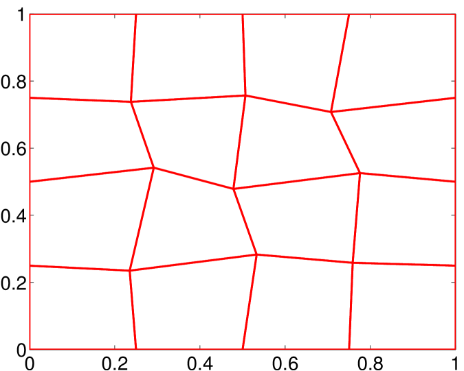
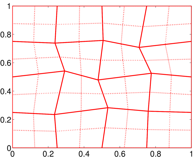
Fig. 1: Mesh level 1 (Left) and mesh level 2 (Right) for example 2.

Table 4: Example 3. Error and rate of convergence for first order WG on quadrilateral meshes.

$h$	${|||}e_{h}{|||}$	order	$\|e_{0}\|$	order
2.9350e-01	1.9612e+00		2.1072e+00
1.4675e-01	1.0349e+00	9.2225e-01	5.7219e-01	1.8808
7.3376e-02	5.2434e-01	9.8094e-01	1.4458e-01	1.9847
3.6688e-02	2.6323e-01	9.9418e-01	3.5655e-02	2.0197
1.8344e-02	1.3179e-01	9.9808e-01	8.6047e-03	2.0509
9.1720e-03	6.5925e-02	9.9934e-01	2.0184e-03	2.0919

Table 5: Example 3. Error and rate of convergence for second order WG on quadrilateral meshes.

$h$	${|||}e_{h}{|||}$	order	$\|e_{0}\|$	order
1/2	1.7955e-01		1.4891e-01
1/4	8.7059e-02	1.0444	1.8597e-02	3.0013
1/8	2.8202e-02	1.6262	2.1311e-03	3.1254
1/16	7.8114e-03	1.8521	2.4865e-04	3.0995
1/32	2.0347e-03	1.9408	2.9964e-05	3.0528
1/64	5.1767e-04	1.9747	3.6806e-06	3.0252
1/128	1.3045e-04	1.9885	4.5627e-07	3.0120

7.3 On Honeycomb Mesh

In the forth test, we solve the Poisson equation on the domain of unit square with exact solution $u=\sin(\pi x)\sin(\pi y)$. The Dirichlet boundary data $g$ and $f$ are chosen to match the exact solution. The numerical experiment is performed on the honeycomb mesh as shown in Figure 2. The linear WG element ($k=1$) is used in this numerical computation.

The error profile is presented in Table 6, which confirms the convergence rates predicted by the theory.

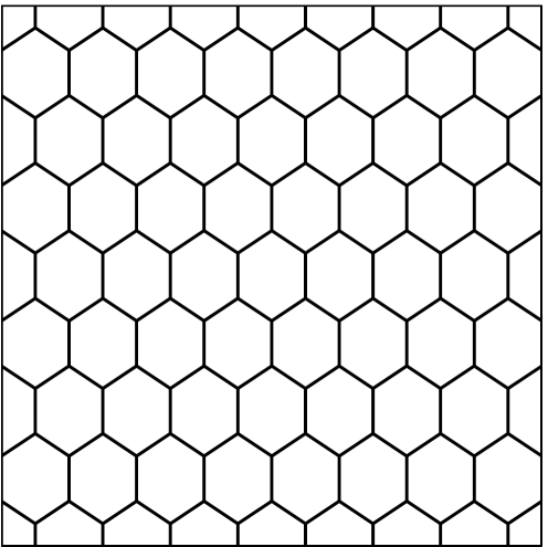
Fig. 2: Honeycomb mesh for example 3.

Table 6: Example 4. Error and rate of convergence for linear WG element on honeycomb meshes.

$h$	${|||}e_{h}{|||}$	order	$\|e_{0}\|$	order
1.6667e-01	3.3201e-01		1.6006e-02
8.3333e-02	1.6824e-01	9.8067e-01	3.9061e-03	2.0347
4.1667e-02	8.4784e-02	9.8867e-01	9.6442e-04	2.0180
2.0833e-02	4.2570e-02	9.9392e-01	2.3960e-04	2.0090
1.0417e-02	2.1331e-02	9.9695e-01	5.9711e-05	2.0047
5.2083e-03	1.0677e-02	9.9839e-01	1.4904e-05	2.0022

7.4 On Deformed Cubic Meshes

In the fifth test, the Poisson equation is solved on a three dimensional domain $\Omega=(0,1)^{3}$. The exact solution is chosen as

$$u=\sin(2\pi x)\sin(2\pi y)\sin(2\pi z),$$

and the Dirichlet boundary date $g$ and $f$ are chosen accordingly to match the exact solution.

Deformed cubic meshes are used in this test, see Figure 3 (Left) for an illustrative element. The construction of the deformed cubic mesh starts with a coarse mesh. The next level of mesh is derived by refining each deformed cube element into $8$ sub-cubes, as shown in Figure 3 (Right). Table 7 reports some numerical results for different level of meshes. It can be seen that a convergent rate of $O(h)$ in $H^{1}$ and $O(h^{2})$ in $L^{2}$ norms are achieved for the corresponding WG finite element solutions. This confirms the theory developed in earlier sections.

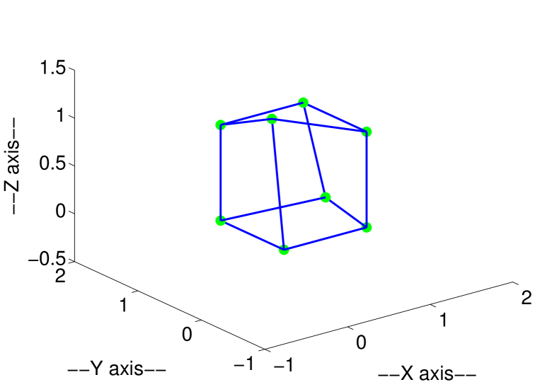
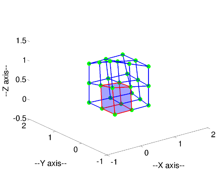
Fig. 3: Mesh level 1 (Left) and mesh level 2 (Right) for example 4.

Table 7: Example 5. Error and convergence rate for $k=1$ on deformed cubic mesh.

$h$	${|||}e_{h}{|||}$	order	$\|e_{0}\|$	order
1/2	5.7522		9.1990
1/4	1.3332	2.1092	1.5684	2.5522
1/8	6.4071e-01	1.0571	2.7495e-01	2.5121
1/16	3.2398e-01	9.8377e-01	6.8687e-02	2.0011
1/32	1.6201e-01	9.9982e-01	1.7150e-02	2.0018

References

• [1] F. Brezzi, J. Douglas, Jr., and L.D. Marini, Two families of mixed finite elements for second order elliptic problems, Numer. Math., 47 (1985), pp. 217-235.
• [2] S. Brenner and R. Scott, The Mathematical Theory of Finite Element Mathods, Springer-Verlag, New York, 1994.
• [3] P.G. Ciarlet, The Finite Element Method for Elliptic Problems, North-Holland, New York, 1978.
• [4] B. Cockburn, J. Gopalakrishnan, and R. Lazarov, Unified hybridization of discontinuous Galerkin, mixed, and continuous Galerkin methods for second order elliptic problems, SIAM J. Numer. Anal. 47 (2009), pp. 1319-1365.
• [5] Q. Li and J. Wang Weak Galerkin Finite Element Methods for Parabolic Equations, arXiv:1212.3637, to appear in the Journal of Numerical Methods for PDEs.
• [6] L. Mu, J. Wang, and X. Ye, Weak Galerkin Finite Element Methods for the Biharmonic Equation on Polytopal Meshes, arXiv:1303.0927.
• [7] P. Raviart and J. Thomas, A mixed finite element method for second order elliptic problems, Mathematical Aspects of the Finite Element Method, I. Galligani, E. Magenes, eds., Lectures Notes in Math. 606, Springer-Verlag, New York, 1977.
• [8] J. Wang and X. Ye, A weak Galerkin finite element method for second-order elliptic problems, J. Comp. and Appl. Math, 241 (2013), pp. 103-115. arXiv:1104.2897v1.
• [9] J. Wang and X. Ye, A weak Galerkin mixed finite element method for second-order elliptic problems, arXiv:1202.3655v2, 2012.