Frozen into stripes: fate of the critical Ising model after a quench

Abstract

In this work we study numerically the final state of the two dimensional ferromagnetic critical Ising model after a quench to zero temperature. Beginning from equilibrium at $T_{c}$, the system can be blocked in a variety of infinitely long lived stripe states in addition to the ground state. Similar results have already been obtained for an infinite temperature initial condition and an interesting connection to exact percolation crossing probabilities has emerged. Here we complete this picture by providing a new example of stripe states precisely related to initial crossing probabilities for various boundary conditions. We thus show that this is not specific to percolation but rather that it depends on the properties of spanning clusters in the initial state.

Introduction — Somewhat surprisingly, even with such a simple set up as the two dimensional nearest neighbour ferromagnetic Ising model quenched to zero temperature, a variety of final states can be reached with non trivial probabilities. It was first noticed by Lipowski Lipowski (1999) that an anomalous scaling for the equilibration time of the kinetic Ising model arises from the existence of stripe states. In an interesting series of papers, Krapivsky, Redner and collaborators noticed as well the presence of stripes states after a quench from infinite temperature, and analysed both the dynamics and the final states. They measured numerically the probability of getting stuck in stripe states and found that it was around $1/3$ but were at first unable to explain it Spirin et al. (2001a, b). In the same situation but with different goals, Sicilia et al. studied the geometry of spin clusters, and noticed that after a few Monte-Carlo steps at $T<T_{c}$, an infinite temperature system on a square lattice is very similar to the critical percolation point for the spin clusters Arenzon et al. (2007); Sicilia et al. (2007). So, even though the initial occupation probability of $1/2$ for a type of spins is inferior to the critical site percolation probability for the square lattice $p_{c}\simeq 0.59$, the system is rapidly very similar to a critical percolation system. This correspondence enabled Krapivsky and collaborators to give an explanation for the probabilities of appearance of stripe states in terms of critical percolation probabilities, be it for free or periodic boundary conditions Barros et al. (2009); Olejarz et al. (2012). The study of these quantities has a long history starting with Cardy and his eponymous formula Cardy (1992). This formula gives the probability of the existence of an incipient spanning cluster at the critical percolation point in terms of hypergeometric functions. Since then a number of percolation probabilities have been studied. One aspect that is particularly interesting is that although Cardy and others found those formulas using conformal field theory (CFT), i.e. in a non rigorous way mathematically speaking, mathematicians have developed rigorous tools to tackle those systems. Schramm introduced the stochastic Loewner evolution (SLE) Schramm (2000) which describes numerous physically occurring curves, and this lead to many results (see Lawler et al. (2002) with Lawler and Werner e.g.). Around the same time, Smirnov proved rigorously Cardy formula and the conformality of the critical percolation point for site percolation on the triangular lattice Smirnov (2001).

The correspondence discovered by Krapivsky et al. is thus very interesting since it relates a non-equilibrium situation to exact results. It is remarkably accurate and based on the observation of Sicilia et al. and general considerations on coarsening dynamics and it was supported by numerical results on a lattice with different aspect ratios. The underlying question to those studies is to what extent the initial condition influences the final one? In this regard, it is interesting to study the same situation with a different initial condition to extract the universal behaviors from the rest. For the Ising model, the results discussed above have to hold for any starting temperature above the critical temperature since for an initial condition at $T>T_{c}$ the long distance properties are governed by the infinite temperature fixed point. Since the subcritical region is trivial from the spin clusters point of view, the critical temperature point only remains and is absolutely non trivial concerning spin clusters as we will disscuss below. Actually, the persistence of the initial condition is also very interesting to study before reaching the final state, i.e. during the equilibration. Several works have dealt with the issue of cluster dynamics after a quench either to $T<T_{c}$ Arenzon et al. (2007); Sicilia et al. (2007) or to $T_{c}$ Blanchard et al. (2012) for the Ising model and for the Potts model Loureiro et al. (2010, 2012) and were able to clarify the influence of the initial condition. Indeed those works show that the initial properties of spin clusters are retained at distances bigger than a dynamical length-scale $\xi(t)\sim t^{1/z}$ using dynamical scaling arguments and numerical checks.

In the following we study the ferromagnetic Ising model whose hamiltonian is written as:

$${\cal H}=-\sum_{\langle ij\rangle}JS_{i}S_{j}\;,$$ (1)

where the sum is over all nearest neighbors pairs of spins of a two dimensional system and $J>0$. The system considered is rectangular and three boundary conditions will be considered : free, periodic and fixed. The lattices used will be discussed in each case.

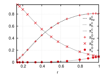
Figure 1: (color online) Crossing probabilities for free boundary conditions versus $r$. The lines corresponding to $\pi^{c}_{h},\pi^{c}_{v}$ and $\pi^{c}_{hv}$ are from the results given in Lapalme and Saint-Aubin (2001) for the critical Ising model. The points correspond to our data for $\pi^{0}_{h},\pi^{0}_{v}$ and $\pi^{0}_{hv}$ obtained after a quench at zero temperature.

Method — In the simulation that we will consider here, we started from a system equilibrated at the critical temperature. The equilibration is obtained with the Wolff cluster algorithm Wolff (1989). We generate a large number of independent configurations, at least one million for each size considered. For each configuration, we determine the probability that there exists at least one cluster of spins crossing the horizontal or vertical direction. We denote these probabilities $\pi^{c}_{h}$ or $\pi^{c}_{v}$. The probability that a spin cluster is crossing in both directions will be denoted $\pi^{c}_{hv}$. Next, we perform a quench at $T=0$. We then let the system evolve with a Glauber dynamics with a suitable algorithm described below until it reaches a stable state. We record similar (stripes) probabilities that we denote by $\pi^{0}_{h},\pi^{0}_{v}$ for the horizontal or vertical stripes and $\pi^{0}_{hv}$ for the stripes in both directions, i.e. a ground state.

One difficulty is that it can take a tremendous amount of (Monte-Carlo) time to reach the final state where no spins can be updated without increasing the energy of the system because the system tends to wander in long-lived iso-energetic states. A simple kinetic Monte Carlo algorithm Bortz et al. (1975) with Glauber dynamics bypasses this issue quite easily. It essentially consists in an efficient sampling of the updateable spins which greatly reduces computation time to reach a final state. In a $T=0$ dynamics, the only possible transition rates on even-coordinated lattices are $0$, $0.5$ and $1$ respectively for spins with strictly more than half of their neighbours of the same colour as theirs, exactly half and strictly less than half. Let us call $n_{+}$, $n_{0}$ and $n_{-}$ the number of spins in this three categories and $R$ the sum of all possible rates, with obviously $R\equiv n_{-}+n_{0}/2$. A list of the $n_{-}+n_{0}$ updateable sites is created. Now, to update the system, a random number $u\in]0,1]$ is drawn, and if $uR\leq n_{-}$, one of the $n_{-}$ spins is flipped and otherwise one among the $n_{0}$ ones. To update the time $t$, we draw another random number $u^{\prime}\in]0,1]$ and $t\leftarrow t+\ln(1/u^{\prime})/R$. Then the list of updateable sites is regenerated and the system can be updated again until $n_{-}+n_{0}=0$.

Free Boundary conditions — We will first describe our results for a system with free boundary conditions. The probabilities $\pi^{c}_{h}$, $\pi^{c}_{v}$ and $\pi^{c}_{hv}$ were already considered in equilibrium at $T_{c}$ by Lapalme and Saint-Aubin Lapalme and Saint-Aubin (2001). These authors measured these quantities on the triangular lattice. They also tried to find a way to predict the behaviour of these crossings in a way analogous to the Cardy formula for percolation. They obtained a differential equation on a four point correlation function related to $\pi^{c}_{h}$ but were unable to solve it so they resorted to a numerical solution in good agreement with their measurements.

We considered systems of size $L\times L/r$ with $L=256$ while varying $r$. We only study the case $r\leq 1$, the case with $r>1$ being obtained by a trivial duality relation exchanging the vertical and horizontal directions. Our results are shown in Fig. 1. In this figure we compare the situation at $T_{c}$ and the final states of the evolution at $T=0$. To do so we present the probabilities of getting a crossing $\pi^{0}_{h},\pi^{0}_{v}$ and $\pi^{0}_{hv}$ for various values of ratio $r$ obtained at $T=0$ as crosses and in the critical case, $\pi^{c}_{h},\pi^{c}_{v}$ and $\pi^{c}_{hv}$ shown as lines. The agreement between the $\pi^{c}$ and the $\pi^{0}$ is excellent, this is one of the main results of the present work. The values of the $\pi^{c}$ are those obtained by Lapalme and Saint-Aubin in Lapalme and Saint-Aubin (2001). Note that these authors considered the case of a triangular lattice while our measurements have been done on a square lattice. As a check, we also repeated the measurement of the $\pi^{c}$ on the square lattice and of the $\pi^{0}$ on the triangular lattice and our results are in perfect agreement with the ones of Lapalme and Saint-Aubin obtained on the triangular lattice. This supports the universality of these quantities.

In conclusion, the crossing probabilities are the same for the equilibrium at $T_{c}$ and in the blocked states obtained after a quench at $T=0$ starting from the critical point. This first result confirms the idea that the final state is dictated by the topology of spin clusters in the initial one.

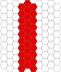
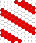
Figure 2: (color online) Two possible types of stripes of the alternate triangular lattice with periodic boundary conditions. The vertical stripes on the left can exist for arbitrary aspect ratios $r$ contrarily to the stripes on the right which only exists for $r=2n/\sqrt{3}$ with $n\in\mathbb{N}^{*}$. Actually the stripe on the right wraps in both directions around the torus.

Periodic Boundary conditions — To make this fact more explicit we move on to the case of periodic boundary condition (PBC). Here the situation is a bit more complicated since clusters can wind in various ways around the torus. We can nonetheless define as previously the percolation probabilities $\pi_{h}^{c}$, $\pi_{v}^{c}$, $\pi_{hv}^{c}$ and $\pi_{h}^{0}$, $\pi_{v}^{0}$, $\pi_{hv}^{0}$ of interest to us. We consider the triangular lattice. With this choice of lattice and boundary condition only vertical stripes are stable at $T=0$ for arbitrary aspects ratios (see Fig. 2). This means that $\pi_{h}^{0}=0$ and $\pi_{hv}^{0}=1-\pi_{v}^{0}$ thus we only need to consider $\pi_{v}^{0}$. As is shown in Fig. 2, diagonal stripes are stable in addition to the vertical ones for the aspect ratios $r=2n/\sqrt{3}$ with $n\in\mathbb{N}^{*}$, but their rarity ($\pi_{\mathrm{diag}}$ is at most $6.10^{-8}$) forbids their study numerically as has been done in Olejarz et al. (2012). The factor $\sqrt{3}/2$ in the definition of the aspect ratio takes into account the actual horizontal system size. We have seen that different percolation probabilities of same spin cluster for free boundary conditions has been studied numerically and analytically in Lapalme and Saint-Aubin (2001). We found no such study for the PBC. This motivated us to extend the work of Arguin Arguin (2002) which deals with the probability that a given configuration contains a Fortuin-Kasteleyn cluster winding $a$ times horizontally and $b$ times vertically around the torus. We have been able to obtain an explicit formula for such a probability for an Ising spin cluster Blanchard (2013). In the case where the spin cluster winds only vertically around the torus, the formula reduces to:

$$\pi^{c}_{v}(r)=\frac{1}{2r|\eta(ir)|}\frac{\theta_{3}\left(\frac{i}{12r}\right)-\theta_{3}\left(\frac{3i}{4r}\right)-2\theta_{2}\left(\frac{3i}{4r}\right)}{|\theta_{2}\left(ir\right)|+|\theta_{3}\left(ir\right)|+|\theta_{4}\left(ir\right)|}$$ (2)

where $\eta$ is the Dedekind $\eta$ function and the $\theta_{i}$ are the Jacobi $\theta$ functions.

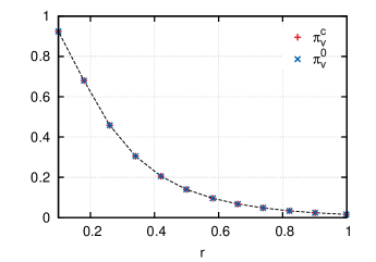
Figure 3: (color online) Vertical percolation probability $\pi_{v}^{c}$ at $T_{c}$ (red crosses) and vertical stripe probability $\pi_{v}^{0}$ at $T=0$ (blue squares) for various aspect ratio $r=L_{y}/(\sqrt{3}L_{x}/2)$ with $L_{y}=128$. The dashed line corresponds to the expression in Eq. (2).

In Fig. 3, the results for the triangular lattice with PBC are presented. The agreement between $\pi^{c}_{v}$, $\pi^{0}_{v}$ (dots) obtained from the simulations and the theoretical prediction from Eq. (2) for $\pi^{c}_{v}$ (dashed line) is very good. This second case confirms the link between probabilities of blocked stripe states and initial crossing probabilities of spin clusters.

Fixed Boundary conditions — Finally, we will look at a last case in which we impose fixed boundary conditions with $S=-1$ on the left and right sides of a rectangle and with $S=+1$ on the top and bottom sides. This case is interesting because it has been extensively studied analytically at $T_{c}$ by several authors using CFT and multiple stochastic Loewner evolutions Arguin and Saint-Aubin (2002); Bauer et al. (2005); Kozdron (2009), so there exists a number of theoretical predictions to compare our simulations to; moreover it is really easy to simulate and analyze as we will see below.

These boundary conditions will force the existence of two interfaces. The two possible configuration types are represented in Fig. 4.

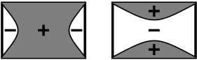
Figure 4: Schematic representation of the two configuration types with fixed boundary conditions. Is is easy to see that beginning with the left (respectively right) configuration we will end up in a state where all spins equal $+1$ ($-1$) except the fixed ones.

In the first case, the first interface goes from the left top corner to the left bottom corner and the second interface connects the right top corner to the bottom right corner. In the second case the interface goes from the left top corner to the right top corner and the second interface connects the bottom left corner to the bottom right corner. The probabilities for these two situations at $T_{c}$ can be written in several equivalent forms, we use Kozdron’s version written only in terms of the hypergeometric function $F$ Kozdron (2009). The probability for the left situation in Fig. 4 is given by:

$$P(x)=\frac{F(\frac{4}{3},3,\frac{8}{3};1-x)}{F(\frac{4}{3},3,\frac{8}{3};x)+F(\frac{4}{3},3,\frac{8}{3};1-x)}$$ (3)

where $x\in(0,1)$ is related to the aspect ratio $r$ by:

$$r=\frac{K(x)}{K(1-x)}$$ (4)

with $K(x)$ the complete elliptic integral of the first kind. For the case of infinite initial temperature, the probabilities for the two situations of Fig. 4 are given by Cardy formula Cardy (1992). Indeed, in the case of percolation, the fixed boundary condition considered in Arguin and Saint-Aubin (2002); Bauer et al. (2005); Kozdron (2009) coincides with the situation considered by Cardy.

As previously we quench the system from $T_{c}$ to $T=0$ but also from $T=\infty$ to $T=0$ as we found no mention of this case in the literature. With this boundary condition the analysis of the final state is really easy, the sign of magnetization suffices to indicate the state of the system as bulk spins are all of the same sign in the end. We show the results of our simulations for $L=1280$ for the initial temperatures $T_{c}$ and $T=\infty$ in Fig. 5. The agreement with the theoretical prediction (dashed lines) is again excellent in both cases.

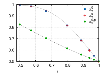
Figure 5: (color online) Crossing probabilities versus $r$. The dashed lines correspond to the formula proved in Arguin and Saint-Aubin (2002); Bauer et al. (2005); Kozdron (2009) for the critical Ising model and in Cardy (1992) for percolation. The symbols correspond to our data for $\pi^{0}_{v}$ (blue filled square) (respectively $\pi^{0,p}_{v}$ (green dots)) obtained after a quench at zero temperature from $T_{c}$ (respectively $T=\infty$). Note that the values measured for $\pi^{c}_{v}$ (red crosses) are indistinguishable from the probability $\pi^{0}_{v}$ since they are numerically very close.

Conclusions — We have extended the connection between crossing probabilities and the probabilities of existence of stripe states after a $T=0$ Glauber dynamics to the case of the critical Ising model for various boundary conditions. We have obtained clear results showing that the final state of the evolution is strongly correlated to the initial condition, similarly to what was already observed in Spirin et al. (2001a, b); Barros et al. (2009); Olejarz et al. (2012) for the quench from $T=\infty$ to $T=0$ in a similar setup. We expect that this is a general feature and it would be interesting to check the generalisation of this result for other models. In a preliminary check, we have obtained similar results for the $Q=3$ Potts model Blanchard et al. (2013). We leave for the future similar studies for more complicated models or even the case of larger dimensions.

ACKNOWLEDGMENTS We thank L. F. Cugliandolo and R. Santachiara for useful discussions and L. F. Cugliandolo for her comments on the manuscript.

References

- Lipowski (1999) A. Lipowski, Physica A 268, 6 (1999).
- Spirin et al. (2001a) V. Spirin, P. Krapivsky, and S. Redner, Phys. Rev. E 65, 016119 (2001a).
- Spirin et al. (2001b) V. Spirin, P. L. Krapivsky, and S. Redner, Phys. Rev. E 63, 036118 (2001b).
- Arenzon et al. (2007) J. J. Arenzon, A. J. Bray, L. F. Cugliandolo, and A. Sicilia, Phy. Rev. Lett. 98, 145701 (2007).
- Sicilia et al. (2007) A. Sicilia, J. J. Arenzon, A. J. Bray, and L. F. Cugliandolo, Phys. Rev. E 76, 061116 (2007).
- Barros et al. (2009) K. Barros, P. L. Krapivsky, and S. Redner, Phys. Rev. E 80, 040101 (2009).
- Olejarz et al. (2012) J. Olejarz, P. L. Krapivsky, and S. Redner, Phys. Rev. Lett. 109, 195702 (2012).
- Cardy (1992) J. L. Cardy, J. Phys. A: Mathematical and General 25, L201 (1992).
- Schramm (2000) O. Schramm, Israel J. Math. 118, 221 (2000).
- Lawler et al. (2002) G. F. Lawler, O. Schramm, and W. Werner, arXiv:math/0204277 (2002).
- Smirnov (2001) S. Smirnov, C.R.A.S. - Series I - Mathematics 333, 239 (2001).
- Blanchard et al. (2012) T. Blanchard, L. F. Cugliandolo, and M. Picco, J. Stat. Mech.: Theory and Experiment 2012, P05026 (2012).
- Loureiro et al. (2010) M. P. O. Loureiro, J. J. Arenzon, L. F. Cugliandolo, and A. Sicilia, Phys. Rev. E 81, 021129 (2010).
- Loureiro et al. (2012) M. P. Loureiro, J. J. Arenzon, and L. F. Cugliandolo, Phys. Rev. E 85, 021135 (2012).
- Lapalme and Saint-Aubin (2001) E. Lapalme and Y. Saint-Aubin, J. Phys. A: Mathematical and General 34, 1825 (2001).
- Wolff (1989) U. Wolff, Phys. Rev. Lett. 62, 361 (1989).
- Bortz et al. (1975) A. Bortz, M. Kalos, and J. Lebowitz, J. Comput. Phys. 17, 10 (1975).
- Arguin (2002) L.-P. Arguin, J. Stat. Phys. 109, 301 (2002).
- Blanchard (2013) T. Blanchard, in prep. (2013).
- Arguin and Saint-Aubin (2002) L.-P. Arguin and Y. Saint-Aubin, Phys. Lett. B 541, 384 (2002).
- Bauer et al. (2005) M. Bauer, D. Bernard, and K. Kytölä, J. Stat. Phys. 120, 1125 (2005).
- Kozdron (2009) M. J. Kozdron, J. Phys. A: Mathematical and Theoretical 42, 265003 (2009).
- Blanchard et al. (2013) T. Blanchard, L. F. Cugliandolo, and M. Picco, in prep. (2013).