The Compressed Annotation Matrix: an Efficient Data Structure for Computing Persistent Cohomology

Abstract.

Persistent homology with coefficients in a field $\mathbb{F}$ coincides with the same for cohomology because of duality. We propose an implementation of a recently introduced algorithm for persistent cohomology that attaches annotation vectors with the simplices. We separate the representation of the simplicial complex from the representation of the cohomology groups, and introduce a new data structure for maintaining the annotation matrix, which is more compact and reduces substancially the amount of matrix operations. In addition, we propose a heuristic to simplify further the representation of the cohomology groups and improve both time and space complexities. The paper provides a theoretical analysis, as well as a detailed experimental study of our implementation and comparison with state-of-the-art software for persistent homology and cohomology.

This article appeared in Algorithmica 2015 [5]. An extended abstract appeared in the proceedings of the European Symposium on Algorithms 2013 [4].

1. Introduction

Persistent homology [14] is an algebraic method for measuring the topological features of a space induced by the sublevel sets of a function. Its generality and stability with regard to noise have made it a widely used tool for the study of data. A common approach is the study of the topological invariants of a nested family of simplicial complexes built on top of the data, seen as a set of points in a geometric space. This approach has been successfully used in various areas of science and engineering, as for example in sensor networks, image analysis, and data analysis where one typically needs to deal with big data sets in high dimensions. Consequently, the demand for designing efficient algorithms and software to compute persistent homology of filtered simplicial complexes has grown.

The first persistence algorithm [15, 23] can be implemented by reducing a matrix defined by face incidence relations, through column operations. The running time is $O(m^{3})$ where $m$ is the number of simplices of the simplicial complex and, despite good performance in practice, Morozov proved that this bound is tight [21]. Recent optimizations taking advantage of the special structure of the matrix to be reduced have led to significant progress in the theoretical analysis [9, 19] as well as in practice [2, 8].

A different approach [11, 12] interprets the persistent homology groups in terms of their dual, the persistent cohomology groups. The cohomology algorithm has been reported to work better in practice than the standard homology algorithm [11] but this advantage seems to fade away when optimizations are employed to the homology algorithms [2]. An elegant description of the cohomology algorithm, using the notion of annotations [7], has been introduced in [13] and used to design more general algorithms for maintaining cohomology groups under simplicial maps.

In this work, we propose an implementation of the annotation-based algorithm for computing persistent cohomology. A key feature of our implementation is a distinct separation between the representation of the simplicial complex and the representation of the cohomology groups. Currently the simplicial complex can be represented either by its Hasse diagram or by using the more compact simplex tree [6]. The cohomology groups are stored in a separate data structure that represents a compressed version of the annotation matrix. As a consequence, the time and space complexities of our algorithm depend mostly on properties of the cohomology groups we maintain along the computation and only linearly on the size of the simplicial complex.

Moreover, maintaining the simplicial complex and the cohomology groups separately allows us to reorder the simplices while keeping the same persistent cohomology. This significantly reduces the size of the cohomology groups to be maintained, and improves considerably both the time and memory performance as shown by our detailed experimental analysis on a variety of examples. Our method compares favorably with state-of-the-art software for computing persistent homology and cohomology.

Background: A simplicial complex is a pair $\mathcal{K}=(V,S)$ where $V$ is a finite set whose elements are called the vertices of $\mathcal{K}$ and $S$ is a set of non-empty subsets of $V$ that is required to satisfy the following two conditions : 1. $p\in V\Rightarrow\{p\}\in S$ and 2. $\sigma\in S,\tau\subseteq\sigma\Rightarrow\tau\in S$. Each element $\sigma\in S$ is called a simplex or a face of $\mathcal{K}$ and, if $\sigma\in S$ has precisely $s+1$ elements ($s\geq-1$), $\sigma$ is called an $s$-simplex and its dimension is $s$. The dimension of the simplicial complex $\mathcal{K}$ is the largest $k$ such that $S$ contains a $k$-simplex. We define $\mathcal{K}^{p}$ to be the set of $p$-dimensional simplices of $\mathcal{K}$, and note its size $|\mathcal{K}^{p}|$. Given two simplices $\tau$ and $\sigma$ in $\mathcal{K}$, $\tau$ is a subface (resp. coface) of $\sigma$ if $\tau\subseteq\sigma$ (resp. $\tau\supseteq\sigma$). The boundary of a simplex $\sigma$, denoted $\partial\sigma$, is the set of its subfaces with codimension $1$.

A filtration [14] of a simplicial complex is an order relation on its simplices which respects inclusion. Consider a simplicial complex $\mathcal{K}=(V,S)$ and a function $\rho:S\rightarrow\mathbb{R}$. We require $\rho$ to be monotonic in the sense that, for any two simplices $\tau\subseteq\sigma$ in $\mathcal{K}$, $\rho$ satisfies $\rho(\tau)\leq\rho(\sigma)$. We will call $\rho(\sigma)$ the filtration value of the simplex $\sigma$. Monotonicity implies that the sublevel sets $\mathcal{K}(r)=\rho^{-1}(-\infty,r]$ are subcomplexes of $\mathcal{K}$, for every $r\in\mathbb{R}$. Let $m$ be the number of simplices of $\mathcal{K}$, and let $(\rho_{i})_{i=1\cdots n}$ be the $n$ different values $\rho$ takes on the simplices of $\mathcal{K}$. Plainly $n\leq m$, and we have the following sequence of $n+1$ subcomplexes:

$$\emptyset=\mathcal{K}_{0}\subseteq\cdots\subseteq\mathcal{K}_{n}=\mathcal{K},\hskip 5.69046pt-\infty=\rho_{0}<\cdots<\rho_{n},\hskip 5.69046pt\mathcal{K}_{i}=\rho^{-1}(-\infty,\rho_{i}]$$

Applying a (co)homology functor to this sequence of simplicial complexes turns

(combinatorial) complexes into (algebraic) abelian groups and inclusion into group homomorphisms. Roughly speaking, a simplicial complex defines a domain as an arrangement of local bricks and (co)homology catches the global features of this domain, like the connected components, the tunnels, the cavities, etc. The homomorphisms catch the evolution of these global features when inserting the simplices in the order of the filtration. Let $H_{p}(\mathcal{K})$ and $H^{p}(\mathcal{K})$ denote respectively the homology and cohomology groups of $\mathcal{K}$ of dimension $p$ with coefficients in a field $\mathbb{F}$. The filtration induces a sequence of homomorphisms in the homology and cohomology groups in opposite directions:

(1.1) $$0=H_{p}(\mathcal{K}_{0})\rightarrow H_{p}(\mathcal{K}_{1})\rightarrow\cdots\rightarrow H_{p}(\mathcal{K}_{n-1})\rightarrow H_{p}(\mathcal{K}_{n})=H_{p}(\mathcal{K})$$

(1.2) $$0=H^{p}(\mathcal{K}_{0})\leftarrow H^{p}(\mathcal{K}_{1})\leftarrow\cdots\leftarrow H^{p}(\mathcal{K}_{n-1})\leftarrow H^{p}(\mathcal{K}_{n})=H^{p}(\mathcal{K})$$

We refer to [14] for an introduction to the theory of homology and persistent homology. Computing the persistent homology of such a sequence consists in pairing each simplex that creates a homology feature with the one that destroys it. The usual output is a persistence diagram, which is a plot of the points $(\rho(\tau),\rho(\sigma))$ for each persistent pair $(\tau,\sigma)$. It is known that because of duality the homology and cohomology sequences above provide the same persistence diagram [12].
The original persistence algorithm [15] considers the homology sequence in Equation 1.1 that aligns with the filtration direction. It detects when a new homology class is born and when an existing class dies as we proceed forward through the filtration. Recently, a few algorithms have considered the cohomology sequence in Equation 1.2 which runs in the opposite direction of the filtration [11, 12, 13]. The birth of a cohomology class coincides with the death of a homology class and the death of a cohomology class coincides with the birth of a homology class. Therefore, by tracking a cohomology basis along the filtration direction and switching the notions of births and deaths, one can obtain all information about the persistent homology of the complex. The algorithm of de Silva et al. [12] computes the persistent cohomology following this principle which is reported to work better in practice than the original persistence algorithm [11]. Recently, Dey et al. [13] recognized that tracking cohomology bases provides a simple and natural extension of the persistence algorithm for filtrations connected with general simplicial maps (and not simply inclusion). Their algorithm is based on the notion of annotation [7] and, when restricted to only inclusions, is a re-formulation of the algorithm of de Silva et al. [12]. Here we follow this annotation based algorithm.

2. Persistent Cohomology Algorithm and Annotations

In this section, we recall the annotation-based persistent cohomology algorithm of [13]. It maintains a cohomology basis under simplex insertions, where representative cocycles are maintained by the value they take on the simplices. We rephrase the description of this algorithm with coefficients in an arbitrary field $\mathbb{F}$, and use standard field notations $\langle\mathbb{F},+,\cdot,-,/,0,1\rangle$.

Definition 2.1.

Given a simplicial complex $\mathcal{K}$, let $\mathcal{K}^{p}$ denote the set of $p$-simplices in $\mathcal{K}$. An annotation for $\mathcal{K}^{p}$ is an assignement $\mathsf{a}^{p}:\mathcal{K}^{p}\rightarrow\mathbb{F}^{g}$ of an $\mathbb{F}$-vector $\mathsf{a}_{\sigma}=\mathsf{a}^{p}(\sigma)$ of same length $g$ for each $p$-simplex $\sigma\in\mathcal{K}^{p}$. We use $\mathsf{a}$ when there is no ambiguity on the dimension. We also have an induced annotation for any $p$-chain $c=\sum_{i}f_{i}\sigma_{i}$ given by linear extension: $\mathsf{a}_{c}=\sum_{i}f_{i}\cdot\mathsf{a}_{\sigma_{i}}$.

Definition 2.2.

An annotation $\mathsf{a}:\mathcal{K}^{p}\rightarrow\mathbb{F}^{g}$ is valid if:
1. $g=\mbox{rank}\,H_{p}(\mathcal{K})$ and 2. two $p$-cycles $z_{1}$ and $z_{2}$ have $\mathsf{a}_{z_{1}}=\mathsf{a}_{z_{2}}$ iff their homology classes $[z_{1}]$ and $[z_{2}]$ are identical.

Proposition 2.3 ([13]).

The following two statements are equivalent:
1. An annotation $\mathsf{a}:\mathcal{K}^{p}\rightarrow\mathbb{F}^{g}$ is valid
2. The cochains $\{\phi_{j}\}_{j=1\cdots g}$ given by $\phi_{j}(\sigma)=\mathsf{a}_{\sigma}[j]$ for all $\sigma\in\mathcal{K}^{p}$ are cocycles whose cohomology classes $\{[\phi_{j}]\}_{j=1\cdots g}$ constitute a basis of $H^{p}(\mathcal{K})$.

A valid annotation is thus a way to represent a cohomology basis. The algorithm for computing persistent cohomology consists in maintaining a valid annotation for each dimension when inserting all simplices in the order of the filtration. Since we process the filtration in a direction opposite to the cohomology sequence (as in Equation 1.2), we discover the death points of cohomology classes earlier than their birth points. To avoid confusion, we still say that a new cocycle (or its class) is born when we discover it for the first time and an existing cocycle (or its class) dies when we see it no more.

We present the algorithm and refer to [13] for its validity. We insert simplices in the order of the filtration. Consider an elementary inclusion $\mathcal{K}_{i}\hookrightarrow\mathcal{K}_{i}\cup\{\sigma\}$, with $\sigma$ a $p$-simplex. Assume that to every simplex $\tau$ of any dimension in $\mathcal{K}_{i}$ is attached an annotation vector $\mathsf{a}_{\tau}$ from a valid annotation $\mathsf{a}$ of $\mathcal{K}_{i}$. We describe how to obtain a valid annotation for $\mathcal{K}_{i}\cup\{\sigma\}$ from that of $\mathcal{K}_{i}$. We compute the annotation $\mathsf{a}_{\partial\sigma}$ for the boundary $\partial\sigma$ in $\mathcal{K}_{i}$ and take actions as follows:

Case 1: If $\mathsf{a}_{\partial\sigma}=0$, $g\leftarrow g+1$ and the annotation vector of any $p$-simplex $\tau\in\mathcal{K}_{i}$ is augmented with a $0$ entry so that $\mathsf{a}_{\tau}=[f_{1},\cdots,f_{g}]^{T}$ becomes $[f_{1},\cdots,f_{g},0]^{T}$. We assign to the new simplex $\sigma$ the annotation vector $\mathsf{a}_{\sigma}=[0,\cdots,0,1]^{T}$. According to Proposition 2.3, this is equivalent to creating a new cohomology class represented by $\phi(\tau)=0$ for $\tau\neq\sigma$ and $\phi(\sigma)=1$.

Case 2: If $\mathsf{a}_{\partial\sigma}\neq 0$, we consider the non-zero element $c_{j}$ of $\mathsf{a}_{\partial\sigma}$ with maximal index $j$. We now look for annotations of those $(p-1)$-simplices $\tau$ that have a non-zero element at index $j$ and process them as follows. If the element of index $j$ of $\mathsf{a}_{\tau}$ is $f\neq 0$, we add $-f/c_{j}\cdot\mathsf{a}_{\partial\sigma}$ to $\mathsf{a}_{\tau}$. Note that, in the annotation matrix whose columns are the annotation vectors, this implements simultaneously a series of elementary row operations, where each row $\phi_{i}$ receives $\phi_{i}\leftarrow\phi_{i}-(\mathsf{a}_{\partial\sigma}[i]/c_{j})\times\phi_{j}$. As a result, all the elements of index $j$ in all columns are now $0$ and hence the entire row $j$ becomes $0$. We then remove the row $j$ and set $g\leftarrow g-1$. $\sigma$ is assigned $\mathsf{a}_{\sigma}=0$. According to Proposition 2.3, this is equivalent to removing the $j^{\text{th}}$ cocycle $\phi_{j}(\tau)=\mathsf{a}_{\tau}[j]$.

As with the original persistence algorithm, the pairing of simplices is derived from the creation and destruction of the cohomology basis elements.

3. Data Structures and Implementation

In this section, we present our implementation of the annotation-based persistent cohomology algorithm. We separate the representation of the simplicial complex from the representation of the cohomology groups.

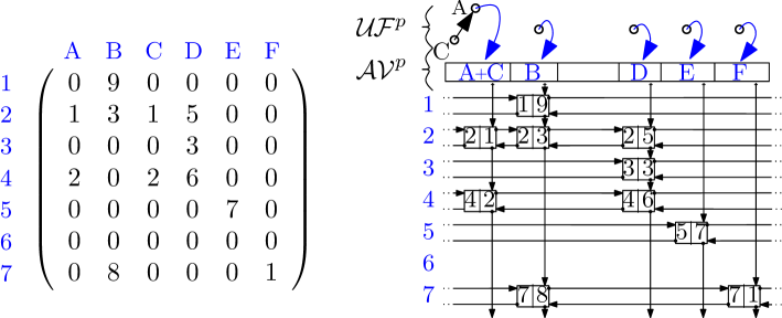
Figure 1. Compressed annotation matrix of a matrix with integer coefficients.

3.1. Representation of the Simplicial Complex

We represent the simplicial complex $\mathcal{K}$ in a data structure $\mathcal{K}_{\text{DS}}$ equipped with the operation Compute-boundary$(\sigma)$ that computes the boundary of a simplex $\sigma$. We denote by $\mathcal{C}_{\partial}^{p}$ the complexity of this operation where $p$ is the dimension of $\sigma$. Additionally, the simplices are ordered according to the filtration.

Two data structures to represent simplicial complexes are of particular interest here. The first one is the Hasse diagram, which is the graph whose nodes are in bijection with the simplices (of all dimensions) of the simplicial complex and an edge links two nodes representing two simplices $\tau$ and $\sigma$ iff $\tau\subseteq\sigma$ and the dimensions of $\tau$ and $\sigma$ differ by $1$. The second data structure is the simplex tree introduced in [6], which is a specific spanning tree of the Hasse diagram. For a simplicial complex $\mathcal{K}$ of dimension $k$ and a simplex $\sigma\in\mathcal{K}$ of dimension $p$, the Hasse diagram has size $O(k|\mathcal{K}|)$ and allows to compute Compute-boundary$(\sigma)$ in time $\mathcal{C}_{\partial}^{p}=O(p)$, whereas the simplex tree has size $O(|\mathcal{K}|)$ and allows to compute Compute-boundary$(\sigma)$ in time $\mathcal{C}_{\partial}^{p}=O(p^{2}D_{\text{m}})$, where $D_{\text{m}}$ is typically a small value related to the time needed to traverse the simplex tree. Both structures can be used in our setting. For readability, we will use a Hasse diagram in the following.

3.2. The Compressed Annotation Matrix

For each dimension $p$, the $p^{\text{th}}$ cohomology group can be seen as a valid annotation for the $p$-simplices of the simplicial complex. Hence, an annotation $\mathsf{a}:\mathcal{K}^{p}\rightarrow\mathbb{F}^{g}$ can be represented as a $g\times|\mathcal{K}^{p}|$ matrix with elements in $\mathbb{F}$, where each column is an annotation vector associated to a $p$-simplex. We describe how to represent this annotation matrix in an efficient way.

Compressing the annotation matrix: In most applications, the annotation matrix is sparse and we store it as illustrated in Figure 1. A column is represented as the singly-linked list of its non-zero elements, where the list contains a pair $(i,f)$ if the $i^{th}$ element of the column is $f\neq 0$. The pairs in the list are ordered according to row index $i$. All pairs $(i,f)$ with same row index $i$ are linked in a doubly-linked list.

Removing duplicate columns: (see Figure 1) To avoid storing duplicate columns, we use two data structures. The first one, ${\mathcal{AV}}^{p}$, stores the annotation vectors and allows fast search, insertion and deletion. ${\mathcal{AV}}^{p}$ can be implemented as a red-black tree or a hash table. We denote by $\mathcal{C}_{{\mathcal{AV}}}^{p}$ the complexity of an operation in ${\mathcal{AV}}^{p}$. For example, if ${\mathcal{AV}}^{p}$ contains $n$ elements and $c_{\text{max}}$ is the length of the longest column, we have $\mathcal{C}_{{\mathcal{AV}}}^{p}=O(c_{\text{max}}\log(n))$ for a red-black tree implementation and $\mathcal{C}_{{\mathcal{AV}}}^{p}=O(c_{\text{max}})$ amortized for a hash-table. The simplices of the same dimension that have the same annotation vector are now stored in a same set and the various (and disjoint) sets are stored in a union-find data structure denoted $\mathcal{U}\mathcal{F}^{p}$. $\mathcal{U}\mathcal{F}^{p}$ is encoded as a forest where each tree contains the elements of a set, the root being the “representative” of the set. The trees of $\mathcal{U}\mathcal{F}^{p}$ are in bijection with the different annotation vectors stored in ${\mathcal{AV}}^{p}$ and the root of each tree maintains a pointer to the corresponding annotation vector in ${\mathcal{AV}}^{p}$. Each node representing a $p$-simplex $\sigma$ in the simplicial complex $\mathcal{K}_{\text{DS}}$ stores a pointer to an element of the tree of $\mathcal{U}\mathcal{F}^{p}$ associated to the annotation vector $\mathsf{a}_{\sigma}$. Finding the annotation vector of $\sigma$ consists in getting the element it points to in a tree of $\mathcal{U}\mathcal{F}^{p}$ and then finding the root of the tree which points to $\mathsf{a}_{\sigma}$ in ${\mathcal{AV}}^{p}$. We avail the following operations on $\mathcal{U}\mathcal{F}^{p}$:

$\bullet$ Create-set: creates a new tree containing one element.

$\bullet$ Find-root: finds the root of a tree, given an element in the tree.

$\bullet$ Union-sets: merges two trees.

The number of elements maintained in $\mathcal{U}\mathcal{F}^{p}$ is at most the number of simplices of dimension $p$, i.e. $|\mathcal{K}^{p}|$. The operations Find-root and Union-sets on $\mathcal{U}\mathcal{F}^{p}$ can be computed in amortized time $O(\alpha(|\mathcal{K}^{p}|))$, where $\alpha(\cdot)$ is the very slowly growing inverse Ackermann function (constant less than $4$ in practice), and Create-set is performed in constant time. We will refer to this data structure as the Compressed Annotation Matrix.

Operations: The compressed annotation matrix described above supports the following operations. We define $c_{\text{max}}$ to be the maximal number of non-zero elements in a column of the compressed annotation matrix (or equivalently in an annotation vector) and $r_{\text{max}}$ to be the maximal number of non-zero elements in a row of the compressed annotation matrix, during the computation. We will express our complexities using $c_{\text{max}}$ and $r_{\text{max}}$:

$\bullet$ Sum-ann$(\mathsf{a}_{1},\mathsf{a}_{2})$: computes the sum of two annotation vectors $\mathsf{a}_{1}$ and $\mathsf{a}_{2}$, and returns the lowest non-zero coefficient if it exists. The column elements are sorted by increasing row index, so the sum is performed in $O(c_{\text{max}})$ time.

$\bullet$ Search-ann/Add-ann/Remove-ann $(\mathsf{a})$: searches, adds or removes an annotation vector $\mathsf{a}$ from ${\mathcal{AV}}^{p}$ in $O(\mathcal{C}_{{\mathcal{AV}}}^{p})$ time.

$\bullet$ Create-cocycle$()$: implements Case 1 of the algorithm described in section 2. It inserts a new column in ${\mathcal{AV}}^{p}$ containing one element $(i_{\text{new}},1)$, where $i_{\text{new}}$ is the index of the created cocycle. This is performed in time $O(\mathcal{C}_{{\mathcal{AV}}}^{p})$. We also create a new disjoint set in $\mathcal{U}\mathcal{F}^{p}$ for the new column. This is done in $O(1)$ time using Create-set. Create-cocycle$()$ takes $O(\mathcal{C}_{{\mathcal{AV}}}^{p})$ in total.

$\bullet$ Kill-cocycle$(\mathsf{a}_{\partial\sigma},c_{j},j)$: implements Case 2 of the algorithm. It finds all columns with a non-zero element at index $j$ and, for each such column $A$, it adds to $A$ the column $-f/c_{j}\cdot\mathsf{a}_{\partial\sigma}$ if $f$ is the non-zero element at index $j$ in $A$. To find the columns with a non-zero element at index $j$, we use the doubly-linked list of row $j$. We call Sum-ann to compute the sums. The overall time needed for all columns is $O(c_{\text{max}}\,r_{\text{max}})$ in the worst-case. Finally, we remove duplicate columns using operations on ${\mathcal{AV}}^{p}$ (in $O(r_{\text{max}}\,\mathcal{C}_{{\mathcal{AV}}}^{p-1})$ time in the worst-case) and call Union-sets on $\mathcal{U}\mathcal{F}^{p-1}$ if two sets of simplices, which had different annotation vectors before calling Kill-cocycle, are assigned the same annotation vector. This is performed in at most $O(r_{\text{max}}\,\alpha(|\mathcal{K}^{p-1}|))$ time. The total cost of Kill-cocycle is $O(r_{\text{max}}(c_{\text{max}}+\mathcal{C}_{{\mathcal{AV}}}^{p-1}+\alpha(|\mathcal{K}^{p-1}|)))$.

3.3. Computing Persistent Cohomology

Given as input a filtered simplicial complex represented in a data structure $\mathcal{K}_{\text{DS}}$, we compute its persistence diagram.

Implementation of the persistent cohomology algorithm: We insert the simplices in the filtration order and update the data structures during the successive insertions. The simplicial complex $\mathcal{K}$ is stored in a simplicial complex data structure $\mathcal{K}_{\text{DS}}$ and we maintain, for each dimension $p$, a compressed annotation matrix, which is empty at the beginning of the computation. For readability, we add the following operation on the set of data structures:

$\bullet$ Compute-${\mathsf{a}_{\partial\sigma}}$($\sigma$): given a $p$-simplex $\sigma$ in $\mathcal{K}$, computes its boundary in $\mathcal{K}_{\text{DS}}$ using Compute-boundary (in $O(\mathcal{C}_{\partial}^{p})$ time). For each of the $p+1$ simplices in $\partial\sigma$, it then finds their annotation vector using Find-root in $\mathcal{U}\mathcal{F}^{p-1}$ (in $O(p\alpha(|\mathcal{K}^{p-1}|))$ time). Finally, it sums all these annotation vectors together (with the appropriate $+/-$ sign) using at most $p+1$ calls to Sum-ann (in $O(p\,g_{\text{m}})$ time). Note that, with the compression method, two simplices in $\partial\sigma$ may point to the same annotation vector; the computation is accelerated by adding such annotation vector only once, with the appropriate multiplicative coefficient. The total worst case complexity of this operation is $O(\mathcal{C}_{\partial}^{p}+p\,\alpha(|\mathcal{K}^{p-1}|)+p\,g_{\text{m}})$.

Let $\sigma$ be a $p$-simplex to be inserted. We compute the annotation vector of $\partial\sigma$ using Compute-${\mathsf{a}_{\partial\sigma}}$. Depending on the value of $\mathsf{a}_{\partial\sigma}$, we call either Create-cocycle or Kill-cocycle. The algorithm computes the pairing of simplices from which one can deduce the persistence diagram. By reversing the pointers from the $\mathcal{U}\mathcal{F}^{p}$s to the simplices in $\mathcal{K}_{\text{DS}}$, one can compute explicitly the representative cocycles of the basis classes and have an explicit representation of the cohomology groups along the computation.

Complexity analysis: Let $k$ be the dimension and $m$ the number of simplices of $\mathcal{K}$. Recall that $c_{\text{max}}$ and $r_{\text{max}}$ represent respectively the maximal number of non-zero elements in an annotation vector and in a row of the compressed annotation matrix, along the computation. Recall that, in dimension $p$, $\mathcal{C}_{\partial}^{p}$ is the complexity of Compute-boundary in $\mathcal{K}_{\text{DS}}$ and $\mathcal{C}_{{\mathcal{AV}}}^{p}$ the complexity of an operation in ${\mathcal{AV}}^{p}$. $\alpha(\cdot)$ is the inverse Ackermann function.

The complexity for inserting $\sigma$ of dimension $p$ is:

$$O\left(\mathcal{C}_{\partial}^{p}+p(\alpha(|\mathcal{K}^{p-1}|)+c_{\text{max}})+\mathcal{C}_{{\mathcal{AV}}}^{p}+r_{\text{max}}(c_{\text{max}}+\mathcal{C}_{{\mathcal{AV}}}^{p-1}+\alpha(|\mathcal{K}^{p-1}|))\right)$$

Consequently, the total cost for computing the persistent cohomology is:

$$O\left(m\times\left[\mathcal{C}_{\partial}^{k}+k(\alpha(m)+c_{\text{max}})+r_{\text{max}}(c_{\text{max}}+\mathcal{C}_{{\mathcal{AV}}}+\alpha(m))\right]\right)$$

Specifically, if we implement $\mathcal{K}_{\text{DS}}$ as a Hasse diagram and the ${\mathcal{AV}}$s as hash-tables, we get $\mathcal{C}_{\partial}^{k}=O(k)$ and $\mathcal{C}_{{\mathcal{AV}}}=O(c_{\text{max}})$. If we consider $\alpha(m)$ as a small constant and remove it for readability, we get that the total cost for computing persistent cohomology is:

$$O(m\,c_{\text{max}}(k+r_{\text{max}}))$$

We show in section 5 that $c_{\text{max}}$ and $r_{\text{max}}$ remain small in practice. Hence, the practical complexity of the algorithm is linear in $m$ for a fixed dimension.

4. Reordering Iso-simplices

Many simplices, called iso-simplices, may have the same filtration value. This situation is common when the filtration is induced by a geometric scaling parameter. Assume that we want to compute the cohomology groups $H^{p}(\mathcal{K}_{i+1})$ from $H^{p}(\mathcal{K}_{i})$ where $\mathcal{K}_{i}\subseteq\mathcal{K}_{i+1}$ and all simplices in $\mathcal{K}_{i+1}\setminus\mathcal{K}_{i}$ have the same filtration value. Depending on the insertion order of the simplices of $\mathcal{K}_{i+1}\setminus\mathcal{K}_{i}$, the dimension of the cohomology groups to be maintained along the computation may vary a lot as well as the computing time. This may lead to a computational bottleneck. We propose a heuristic to reorder iso-simplices and show its practical efficiency in Section 5.

Intuitively, we want to avoid the creation of many “holes” of dimension $p$ and want to fill them up as soon as possible with simplices of dimension $p+1$. For example, in Figure 2, we want to avoid inserting all edges first, which will create two holes that will be filled when inserting the triangles. To do so, we look for the maximal faces to be inserted and recursively insert their subfaces. We conduct the recursion so as to minimize the maximum number of holes. In addition, to avoid the creation of holes due to maximal simplices that are incident, maximal simplices sharing subfaces are inserted next to each other.

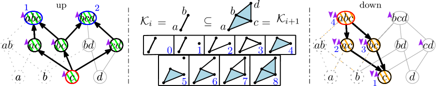
Figure 2. Inclusion $\mathcal{K}_{i}\subseteq\mathcal{K}_{i+1}$. Left: upward traversal (in green) from simplex $\{c\}$. The ordering of the maximal cofaces appears in blue. Right: downward traversal (in orange) from simplex $\{abc\}$. The ordering of the subfaces appears in blue.

We can describe the reordering algorithm in terms of a graph traversal. The graph considered is the graph of the Hasse diagram of $\mathcal{K}_{i+1}\setminus\mathcal{K}_{i}$, defined in section 3.1 (see Figure 2).

Let $\sigma_{1}\cdots\sigma_{\ell}$ be the iso-simplices of $\mathcal{K}_{i+1}\setminus\mathcal{K}_{i}$, sorted so as to respect the inclusion order. We attach to each simplex two flags, a flag $F_{\text{up}}$ and a flag $F_{\text{down}}$, set to 0 originally. When inserting a simplex $\sigma_{j}$, we proceed as follows. We traverse the Hasse diagram upward in a depth-first fashion and list the inclusion-maximal cofaces of $\sigma_{j}$ in $\mathcal{K}_{i+1}\setminus\mathcal{K}_{i}$. The flags $F_{\text{up}}$ of all traversed nodes are set to 1 and the maximal cofaces are ordered according to the traversal. From each maximal coface in this order, we then traverse the graph downward and order the subfaces in a depth-first fashion: this last order will be the order of insertion of the simplices. The flags $F_{\text{down}}$ of all traversed nodes are set to 1. We stop the upward (resp. downward) traversal when we encounter a node whose flag $F_{\text{up}}$ (resp. $F_{\text{down}}$) is set to 1. We do not insert either simplices that have been inserted previously.

By proceeding as above on all simplices of the sequence $\sigma_{1}\cdots\sigma_{\ell}$, we define a new ordering which respects the inclusion order between the simplices. Indeed, as the downward traversal starts from a maximal face and is depth first, a face is always inserted after its subfaces. Every edge in the graph is traversed twice, once when going upward and the other when going downward. Indeed, during the upward traversal, at each node $N$ associated to a simplex $\sigma_{N}$, we visit only the edges between $N$ and the nodes associated to the cofaces of $\sigma_{N}$ and, during the downward traversal, we visit only the edges between $N$ and the nodes associated to the subfaces of $\sigma_{N}$. If $\mathcal{K}_{i+1}\setminus\mathcal{K}_{i}$ contains $\ell$ simplices, the reordering takes in total $O(\ell\times(\mathcal{C}_{\partial}+\mathcal{C}_{co\partial}))$ time, where $\mathcal{C}_{\partial}$ (resp. $\mathcal{C}_{co\partial}$) refers to the complexity of computing the codimension $1$ subfaces (resp. cofaces) of a simplex in the simplicial complex data structure $\mathcal{K}_{\text{DS}}$. The reordering of the filtration can either be done as a preprocessing step if the whole filtration is known, or on-the-fly as only the neighboring simplices of a simplex need to be known at a time. The reordering of a set of iso-simplices respects the inclusion order of the simplices and the filtration, and therefore does not change the persistence diagram of the filtered simplicial complex. This is a direct consequence of the stability theorem of persistence diagrams [10]. However, it may change the pairing of simplices.

5. Experiments

In this section, we report on the experimental performance of our implementation. The compressed annotation matrix implementation of persistent cohomology (denoted by CAM in the following) is part of the Gudhi library [16, 17, 18, 22].

Given a filtered simplicial complex as input, we measure the time taken by our implementation to compute its persistent cohomology, and provide various statistics. We compare the timings with state-of-the-art software computing persistent homology and cohomology. Specifically, we compare our implementation with the Dionysus library [20] which provides implementation for persistent homology [15, 23] and persistent cohomology [12] (denoted DioCoH) with field coefficients in $\mathbb{Z}_{p}$, for any prime $p$. We also compare our implementation with the PHAT library (version 1.4) [1, 3] which provides an implementation of the optimized algorithm for persistent homology [2, 8] (using the --twist option) as well as an implementation of persistent cohomology [2, 11] (using the --dualize option), with coefficients in $\mathbb{Z}_{2}$ only. DioCoH and PHAT have been reported to be the most efficient implementation in practice [2, 11]. All timings are measured on a Linux machine with $3.00$ GHz processor and $32$ GB RAM. Dionysus, PHAT and our implementation are written in C++ and compiled with gcc 4.6.2 with optimization level -O3. Timings are all averaged over $10$ independent runs. The symbols $\text{T}_{\infty}$ means that the computation lasted more than $12$ hours.

DioCoH

PHAT⟂

PHAT

CAM

Data	Cpx	$|\mathcal{P}|$	$D$	$d$	$\rho_{\text{max}}$	$k$	$|\mathcal{K}|$	$\mathbb{Z}_{2}$	$\mathbb{Z}_{11}$	$\mathbb{Z}_{2}$	$\mathbb{Z}_{11}$	$\mathbb{Z}_{2}$	$\mathbb{Z}_{11}$	$\mathbb{Z}_{2}$	$\mathbb{Z}_{11}$
Cy8	Rips	$6040$	$24$	$2$	$0.41$	$16$	$21\times 10^{6}$	$420$	$4822$	$44$	$-$	$5.4$	$-$	$6.4$	$6.5$
S4	Rips	$507$	$5$	$4$	$0.715$	$5$	$72\times 10^{6}$	$943$	$1026$	$96$	$-$	$3554$	$-$	$22.5$	$23.2$
L57	Rips	$4769$	$-$	$3$	$0.02$	$3$	$34\times\par 10^{6}$	$239$	$240$	$35$	$-$	$970$	$-$	$9.3$	$9.5$
Bro	Wit	$500$	$25$	?	$0.06$	$18$	$3.2\times 10^{6}$	$807$	$\text{T}_{\infty}$	$6.5$	$-$	$0.88$	$-$	$2.7$	$2.9$
Kl	Wit	$10000$	$5$	$2$	$0.105$	$5$	$74\par\times 10^{6}$	$569$	$662$	$100$	$-$	$1771$	$-$	$19.7$	$19.9$
L35	Wit	$700$	$-$	$3$	$0.06$	$3$	$18\times\par 10^{6}$	$109$	$110$	$18$	$-$	$865$	$-$	$5.1$	$5.1$
Bud	$\alpha$Sh	$49990$	$3$	$2$	$\infty$	$3$	$1.4\times 10^{6}$	$30.0$	$30.9$	$2.5$	$-$	$0.33$	$-$	$0.7$	$0.7$
Nep	$\alpha$Sh	$2\times 10^{6}$	$3$	$2$	$\infty$	$3$	$57\times 10^{6}$	$\text{T}_{\infty}$	$\text{T}_{\infty}$	$166$	$-$	$33$	$-$	$39.5$	$40.2$

Figure 3. Data, timings (in seconds) and statistics.

We construct three families of simplicial complexes [14] which are of particular interest in topological data analysis: the Rips complexes (denoted Rips), the relaxed witness complexes (denoted Wit) and the $\alpha$-shapes (denoted $\alpha$Sh). These complexes depend on a relaxation parameter $\rho$. When the data points are embedded, the complexes are constructed up to embedding dimension, with euclidean metric. They are constructed up to the intrinsic dimension of the space with intrinsic metric otherwise. We use a variety of both real and synthetic datasets: Cy8 is a set of points in $\mathbb{R}^{24}$, sampled from the space of conformations of the cyclo-octane molecule, which is the union of two intersecting surfaces; S4 is a set of points sampled from the unit $4$-sphere in $\mathbb{R}^{5}$; L57 and L35 are sets of points in the lens spaces $L(5,7)$ and $L(3,5)$ respectively, which are non-embedded spaces; Bro is a set of $5\times 5$ high-contrast patches derived from natural images, interpreted as vectors in $\mathbb{R}^{25}$, from the Brown database; Kl is a set of points sampled from the surface of the figure eight Klein Bottle embedded in $\mathbb{R}^{5}$; Bud is a set of points sampled from the surface of the Happy Buddha (http://graphics.stanford.edu/data/3Dscanrep/) in $\mathbb{R}^{3}$; and Nep is a set of points sampled from the surface of the Neptune statue (http://shapes.aimatshape.net/). Datasets are listed in Figure 3 with details on the sets of points $\mathcal{P}$, their size $|\mathcal{P}|$, the ambient dimension $D$, the intrinsic dimension $d$ of the object the sample points belong to (if known), the threshold $\rho_{\text{max}}$, the dimension $k$ of the simplicial complexes and the size $|\mathcal{K}|$ of the simplicial complexes.

Time Performance: As Dionysus and PHAT encode explicitely the boundaries of the simplices, we use a Hasse diagram for implementing $\mathcal{K}_{\text{DS}}$. We thus have the same time complexity for accessing the boundaries of simplices. We use the persistent homology algorithm of PHAT with options --twist --sparse_pivot_column and the persistent cohomology algorithm (noted PHAT^⟂) with option --twist --sparse_pivot_column --dualize. The --twist algorithm is the most efficient for our experiments. The --sparse_pivot_column representation for the ”pivot column” is the most efficient representation, for our experiemnts, that can generalize to arbitrary coefficients for persistent homology. As illustrated in Figure 3, the persistent cohomology algorithm of Dionysus is always several times slower than our implementation. Moreover, DioCoH is sensitive to the field used, as illustrated in the case of Cy8 and Bro. On the contrary, CAM shows almost identical performance for $\mathbb{Z}_{2}$ and $\mathbb{Z}_{11}$ coefficients on all examples. The persistent cohomology algorithm PHAT^⟂ performs better than DioCoH. However, CAM is still between $2.3$ and $6.9$ times faster.

The persistent homology algorithm of PHAT shows good performance in the case of the alpha shapes and on Cy8 and Bro: CAM and PHAT have close timings. However, CAM scales better to more complex examples (such as S4, L57, Kl and L35, which have higher intrinsic dimension and more complex topology). Indeed, the running time per simplex of CAM remains stable on all examples and for all field coefficients (between $2.7\times 10^{-7}$ and $9.1\times 10^{-7}$ seconds per simplex).

Nep $|M|$ $\#\mathbb{F}op.$ Compression $126057$ $84\times 10^{6}$ $\neg$Compression $574426$ $3860\times 10^{6}$

Nep average maximum $c_{\text{av}},c_{\text{max}}$ $0.79$ $18$ $r_{\text{av}},r_{\text{max}}$ $1.02$ $18$

Bro time Reordering $2.9$ s. $\neg$Reordering $14.2$ s.

Bro $\mathbb{Z}_{11}$ $\mathbb{Q}$ $M_{\text{DS}}$ $\mathsf{a}_{\partial\sigma}$ $M_{\text{op}}$ $M_{\text{DS}}$ $\mathsf{a}_{\partial\sigma}$ $M_{\text{op}}$ $71\%$ $19\%$ $10\%$ $67\%$ $21\%$ $12\%$

Figure 4. Statistics on the effect of the optimizations.

Statistics and Optimization: Figure 4 presents statistics about the computation. The top table presents, on the left, the effect of the compression (removal of duplicate columns) of the annotation matrix on the number of elements $|M|$ stored in the sparse representation and the number of changes $\#\mathbb{F}op.$ in the matrix during the computation of the persistence diagram of Nep. We note a reduction factor of $4.5$ for the size of the matrix, and we proceed to $46$ times less field operations with the compression. Considering Nep is $57$ million simplices, we proceed to less than $1.5$ field operations per simplex on average. The right part of the table shows the average and maximum number of non-zero elements in a column when proceeding to a sum of annotation vectors (Sum-ann) and the average and maximum number of non-zero elements in a row when proceeding to its reduction (Kill-cocycle). These values are key variables ($c_{\text{max}}$ and $r_{\text{max}}$ respectively) in the complexity analysis of the algorithm. We note that these values remain really small. The bottom table presents the effect of the reordering strategy on the example Bro. We note that reordering iso-simplices makes the computation $4.9$ faster. Finally, the right side of the table presents how the computing time is divided into maintaining the compressed annotation matrix (noted $M_{DS}$), computing the annotation vector $\mathsf{a}_{\partial\sigma}$ and modifying the values of the elements in the compressed annotation matrix (noted $M_{\text{op}}$). The percentage are given when computing persistent cohomology with $\mathbb{Z}_{11}$ and $\mathbb{Q}$ coefficients. The computational complexity of field operations $\langle\mathbb{F},+,\cdot,-,/,0,1\rangle$ depends on the field we use. For $\mathbb{Z}_{11}$, or any field of small cardinality, the operations can be precomputed and accessed in constant time. The field operations in $\mathbb{Q}$ are more costly. Specifically, an element $q$ in $\mathbb{Q}$ is represented as a pair of coprime integers $(r,s)$ such that $q=r/s$, and field operations may require gcd computation to ensure that nominator and denominator remain coprime. However, the computational time of CAM is quite insensitive to the field we use. Specifically, as it minimizes the number of matrix changes using the compression method, the computational time is only increased by $8\%$ when computing persistence with $\mathbb{Q}$ coefficients instead of $\mathbb{Z}_{11}$, whereas the computation involving field operations takes $34\%$ more time.

In all our experiments, the size of the compressed annotation matrix is negligible compared to the size of the simplicial complex. Consequently, combined with the simplex tree data structure [6] for representing the simplicial complex, we have been able to compute the persistent cohomology of simplicial complexes of several hundred million simplices in high dimension.

Acknowledgement: The research leading to these results has received funding from the European Research Council (ERC) under the European Union’s Seventh Framework Programme (FP/2007-2013) / ERC Grant Agreement No. 339025 GUDHI (Algorithmic Foundations of Geometry Understanding in Higher Dimensions).

This research is also partially supported by the 7th Framework Programme for Research of the European Commission, under FET-Open grant number 255827 (CGL Computational Geometry Learning). This research is also partially supported by NSF (National Science Foundation, USA) grants CCF-1048983 and CCF-1116258.

References

- [1] Ulrich Bauer, Michael Kerber, and Jan Reininghaus. PHAT, 2013. https://code.google.com/p/phat/.
- [2] Ulrich Bauer, Michael Kerber, and Jan Reininghaus. Clear and compress: Computing persistent homology in chunks. In Topological Methods in Data Analysis and Visualization III, pages 103–117. 2014.
- [3] Ulrich Bauer, Michael Kerber, Jan Reininghaus, and Hubert Wagner. PHAT - persistent homology algorithms toolbox. In Mathematical Software - ICMS 2014 - 4th International Congress, Seoul, South Korea, August 5-9, 2014. Proceedings, pages 137–143, 2014.
- [4] Jean-Daniel Boissonnat, Tamal K. Dey, and Clément Maria. The compressed annotation matrix: An efficient data structure for computing persistent cohomology. In Algorithms - ESA 2013 - 21st Annual European Symposium, Sophia Antipolis, France, September 2-4, 2013. Proceedings, pages 695–706, 2013.
- [5] Jean-Daniel Boissonnat, Tamal K. Dey, and Clément Maria. The compressed annotation matrix: An efficient data structure for computing persistent cohomology. Algorithmica, 73(3):607–619, 2015.
- [6] Jean-Daniel Boissonnat and Clément Maria. The simplex tree: An efficient data structure for general simplicial complexes. Algorithmica, 70(3):406–427, 2014.
- [7] Oleksiy Busaryev, Sergio Cabello, Chao Chen, Tamal K. Dey, and Yusu Wang. Annotating simplices with a homology basis and its applications. In SWAT, pages 189–200, 2012.
- [8] Chao Chen and Michael Kerber. Persistent homology computation with a twist. In Proceedings 27th European Workshop on Computational Geometry, 2011.
- [9] Chao Chen and Michael Kerber. An output-sensitive algorithm for persistent homology. Comput. Geom., 46(4):435–447, 2013.
- [10] David Cohen-Steiner, Herbert Edelsbrunner, and John Harer. Stability of persistence diagrams. Discrete & Computational Geometry, 37(1):103–120, 2007.
- [11] Vin de Silva, Dmitriy Morozov, and Mikael Vejdemo-Johansson. Dualities in persistent (co)homology. CoRR, abs/1107.5665, 2011.
- [12] Vin de Silva, Dmitriy Morozov, and Mikael Vejdemo-Johansson. Persistent cohomology and circular coordinates. Discrete & Computational Geometry, 45(4):737–759, 2011.
- [13] Tamal K. Dey, Fengtao Fan, and Yusu Wang. Computing topological persistence for simplicial maps. In Symposium on Computational Geometry, page 345, 2014.
- [14] Herbert Edelsbrunner and John Harer. Computational Topology - an Introduction. American Mathematical Society, 2010.
- [15] Herbert Edelsbrunner, David Letscher, and Afra Zomorodian. Topological persistence and simplification. Discrete & Computational Geometry, 28(4):511–533, 2002.
- [16] Clément Maria. Filtered complexes. In GUDHI User and Reference Manual. GUDHI Editorial Board, 2015.
- [17] Clément Maria. Persistent cohomology. In GUDHI User and Reference Manual. GUDHI Editorial Board, 2015.
- [18] Clément Maria, Jean-Daniel Boissonnat, Marc Glisse, and Mariette Yvinec. The Gudhi library: Simplicial complexes and persistent homology. In International Congress on Mathematical Software, pages 167–174, 2014.
- [19] Nikola Milosavljevic, Dmitriy Morozov, and Primoz Skraba. Zigzag persistent homology in matrix multiplication time. In Symposium on Comp. Geom., 2011.
- [20] Dmitriy Morozov. Dionysus. http://www.mrzv.org/software/dionysus/.
- [21] Dmitriy Morozov. Persistence algorithm takes cubic time in worst case. BioGeometry News, Dept. Comput. Sci., Duke Univ, 2005.
- [22] The GUDHI Project. GUDHI User and Reference Manual. GUDHI Editorial Board, 2015.
- [23] Afra Zomorodian and Gunnar E. Carlsson. Computing persistent homology. Discrete & Computational Geometry, 33(2):249–274, 2005.