Subspace-preserving sparsification of matrices with minimal perturbation to the near null-space. Part II: Approximation and Implementation

Abstract

This is the second of two papers to describe a matrix sparsification algorithm that takes a general real or complex matrix as input and produces a sparse output matrix of the same size. The first paper [1] presented the original algorithm, its features, and theoretical results.

Since the output of this sparsification algorithm is a matrix rather than a vector, it can be costly in memory and run-time if an implementation does not exploit the structural properties of the algorithm and the matrix. Here we show how to modify the original algorithm to increase its efficiency. This is possible by computing an approximation to the exact result. We introduce extra constraints that are automatically determined based on the input matrix. This addition reduces the number of unknown degrees of freedom but still preserves many matrix subspaces. We also describe our open-source library that implements this sparsification algorithm and has interfaces in C++, C, and MATLAB.

1 Introduction

In the first paper of this series [1], we presented a matrix-valued linearly constrained convex quadratic optimization problem. The application was to compute a sparsified matrix from a dense input matrix such that the sparsification process led to small perturbations in the lower end of the spectrum and preserved the null-spaces and some other important properties of input matrix.

Our first objective here is to describe an enhancement that leads to an approximate solution using less computational time. The second objective is to describe our open-source library, named TxSSA, that implements the sparsification algorithm and is usable from C++, C, and MATLAB. We also add to the theoretical and numerical results presented earlier.

We briefly mention the original optimization problem. Given a matrix $A\in\mathbb{\mathbb{C}}^{m\times n}$, we want to compute a sparse $X\in\mathbb{\mathbb{C}}^{m\times n}$, that solves the following problem.

$$\min_{X} \frac{1}{2}\left|\left|(X-A){A}^{\dagger}\right|\right|^{2}_{F}+\frac{1}{2}\left|\left|{A}^{\dagger}(X-A)\right|\right|^{2}_{F}\text{ such that }$$

$$\mathcal{N}(A)\subseteq\mathcal{N}(X),$$

$$\mathcal{N}(A^{*})\subseteq\mathcal{N}(X^{*}),\text{ and }$$

$$X\text{ has a specified sparsity pattern. }$$ (1)

The symbol $\dagger$ is for Moore-Pensrose pseudoinverse, $*$ is for Hermitian transpose, and $\mathcal{N}$ denotes the null-space of a matrix. Typically the sparsity pattern is computed from $A$ but could be specified separately. In the first paper, we described an $L_{p}$ norm based algorithm for sparsity pattern determination that works on individual rows and columns to preserves entries with large magnitude.

Here is an outline of this paper. In Section 2, we describe some computational issues with the optimization problem. In Section 3, we describe a solution to rectify these issues, which is an algorithm to specify extra constraints in the optimization problem. In Section 4, we deal with existence and uniqueness issues. In Section 5, we show that specification of extra constraints still preserves useful matrix properties. We give details of the numerical techniques we use in Section 6. In Section 7, we describe our implementation of the sparsification algorithm. Finally, in Section 8, we show some new numerical results related to the enhancements we propose in this paper.

2 Computational issues with sparsification

The sparsification problem discussed in [1] and in Equation (1) is mathematically simple because it is a linearly constrained quadratic convex minimization problem. The inputs are the Moore-Penrose pseudoinverse of input matrix $A$ and the desired sparsity pattern $\mathcal{Z}(X)$. We have algorithms to compute them. However, the optimization problem is computationally expensive. There are multiple reasons for this.

1. The number of unknowns, which is equal to number of non-zeros in the sparsity pattern, can be significantly larger than $m$ or $n$, the input and output matrix sizes.

2. The conditioning of the Hessian can be significantly worse compared to the conditioning of the input matrix. This is evident by looking at the eigenvalue decomposition of the Kronecker sum Hessian, as shown in [1, Section 2.6].

3. The graph corresponding to the Hessian does not necessarily have the structure required for sparse direct solvers to be efficient. Typically they lead to large fill-in even after fill-in reducing permutations are applied.

See Section 8 for a numerical example showing these phenomena. The minimization problem is still solvable but the cost grows rapidly with matrix size. Our goal is to control the minimization cost.

Our solution, described ahead in detail, is to reduce the number of unknowns by imposing simple linear equality constraints. The size of the reduced Hessian is then small enough to be factored by a dense solver. Although this changes the original problem and so we do not compute the exact solution. We will show in Section 8 that the effect of such an approximation is minor.

We call this process, using which we reduce the number of unknowns, binning. It is a mathematically well-defined process and requires an input parameter for number of bins. However, the results are not too sensitive once the parameter is sufficiently large. By reducing system size, binning typically improves the conditioning of the optimization problem so that is one less issue to worry about too. In an earlier paper of ours [2], we had not done any binning and had to resort to iterative solvers and early termination to manage the speed of our algorithm. Similarly, in [3], which was the original work for such a sparsification algorithm, black-box dense matrix solvers were used to invert all matrices. Simply speaking, the focus was on prototyping the features of the algorithm rather than the solver. These limitations are now removed as well.

3 Binning the unknown entries

The concept of binning the unknowns is simple. It is based on the numerical evidence that when the exact minimization problem is solved, the matrix locations that are nearly equal in value in the input matrix $A$ remain nearly equal in value in the output matrix $X$ (when present in the sparsity pattern). This holds for entries belonging to different rows and columns. See [1, Section 6] for an example.

We use this observation to enforce extra linear equality constraints a priori between the entries of $X$ if the corresponding entries in $A$ are nearly equal. Since these are very simple constraints, it is easy to eliminate one unknown and reduce the problem size by one (per constraint). Of course, multiple entries of $A$ can be nearly equal in which case multiple corresponding unknown $X$ entries are constrained to be in one bin. Hence the name of the process. We typically reduce the problem size so that it contains a few hundred bins, for arbitrary sparsity patterns. Once the reduced Hessian is formed, such a problem can be solved very quickly.

The main question is whether enforcing so many extra constraints via binning will lead to a matrix $X$ which has suitable spectral properties and is subspace-preserving. This is a topic of other theoretical sections ahead and some numerical results are presented in in Section 8. It is seen that the constraints due to binning conflict with the constraints due to null-spaces in general (when the left or right null-spaces are non-trivial). We show how to avoid this issue and still get a suitable matrix $X$. First, we present a detailed description of the binning algorithm ignoring its effects on optimization.

3.1 A binning algorithm

The input to the binning algorithm is the matrix $A\in\mathbb{\mathbb{R}}^{m\times n}$ or $A\in\mathbb{\mathbb{C}}^{m\times n}$, the chosen sparsity pattern $\mathcal{Z}(A)\in\mathbb{\mathbb{R}}^{m\times n}$, and the maximum number of bins $N_{bin}$ per real or imaginary part. If the matrices are complex, the sparsity pattern is the same for both, real and imaginary, parts. This is by design, see [1, Remark 3.10]. But we keep $N_{bin}$ bins for the real part and $N_{bin}$ bins for the imaginary part and they are binned separately.

The output of the binning algorithm is one bin identifier corresponding to each non-zero in $\mathcal{Z}(A)$, per real and imaginary part. A bin identifier is a natural number. Unknowns with the same bin identifier will be constrained to be equal in the optimization process. For complex matrices, bin identifiers for real and imaginary parts don’t overlap. Essentially, we choose the smallest bin identifier for the imaginary part to be one greater than the largest bin identifier for the real part.

Let $\mathcal{B}(A)$ denote the bin identifier matrix, which is of the same size as $A$. It is real if $A$ is real and complex if $A$ is complex. All entries of $\mathcal{B}(A)$ are non-negative integers. Our convention is that $(\mathcal{B}(A))_{ij}=0$ if $(\mathcal{Z}(A))_{ij}=0$, in which case it is not a bin identifier.

Here is a basic binning algorithm in detail. First we take all the entries of $A$ whose corresponding entry in $\mathcal{Z}(A)$ is one and compute their minimum and maximum value. This gives use the range. The range is equally divided to form $N_{bin}$ bins and each entry is then placed in a bin. When all entries are binned, some bins may remain empty and no identifier is assigned to them. The non-empty bins are given an identifier sequentially. All the matrix locations that fall in the same bin will be constrained to be equal while optimizing.

As a simple example, a bin identifier can be computed by a simple formula as follows. Here $v$ is the real value for which an identifier is to be computed, $\min$ is the minimum matrix value, $\max$ is the maximum matrix value, and $h$ is $\frac{\max-\min}{N_{bin}}$.

$$id=\lfloor(v-\min)h\rfloor+1$$

We compute such identifiers separately for the positive and negative ranges in the input matrix.

Here is a concrete example using a $3\times 4$ real matrix that shows the process of computing the sparsity pattern and bin identifiers.

    A =  5     4     1    -5
        -5     8    -7     7
         0     9    -7    -5

    A_pat = full(p_norm_sparsity_matrix(A, 0.6, 1));
         1     0     0     1
         1     1     1     1
         0     1     1     1

    A_id = full(bin_sparse_matrix(A, A_pat, 8))
         1     0     0     2
         2     3     2     3
         0     3     2     2

For this example, the sparsity ratio is 0.6, $p$ for $L_{p}$ norm is 1, and maximum number of bins is 8. The function names and arguments correspond to the MATLAB implementation (Section 7.2). Note that $N_{bin}$ refers to maximum number of bins and the actual number of bins can be less than that, three in this example.

The binning process can also be visually described using the MATLAB command sortrows. We sort A and A_id values together after vectorization.

  B = sortrows([A(:) A_id(:)])’

   -7 -6 -5 -5 -5  0  1  4  5  7  8  9
    2  2  2  2  2  0  0  0  1  3  3  3

This clearly shows that values close to each other are assigned equal bins and that bins for values not in the sparsity pattern are 0.

The binning algorithm is designed to satisfy some important properties. They are listed below without proofs. To simplify the discussion ahead, we define the notion of equivalence of bin identifier matrices. The letters $i,j,k,$ and $l$ are indices within appropriate ranges.

Definition 3.1.

Two real bin identifier matrices $\mathcal{B}^{1}$ and $\mathcal{B}^{2}$ are equivalent, denoted by $\mathcal{B}^{1}\sim\mathcal{B}^{2}$, if and only if they are of the same size and $(\mathcal{B}^{1})_{ij}=(\mathcal{B}^{1})_{kl}$ whenever $(\mathcal{B}^{2})_{ij}=(\mathcal{B}^{2})_{kl}$. For complex bin identifier matrices, the equivalence holds if the real and imaginary parts are equivalent individually.

We use the notion of equivalence rather than true equality because we do not care about permutation of bin identifiers. We only care about whether they lead to the same subspace when all binning related constraints are imposed.

We now state a few important properties related to binning using conventions mentioned above and the definition of equivalence. The proofs are elementary and we skip them. The matrix $A$ can be be real or complex.

1. $A_{ij}=0\implies(\mathcal{B}(A))_{ij}=0$.

2. $\mathcal{B}(\alpha A)\sim\mathcal{B}(A)$ for $\alpha\in\mathbb{R}\setminus\{0\}$.

3. $\mathcal{B}(A^{T})\sim(\mathcal{B}(A))^{T}$.

4. $\mathcal{B}(A^{*})\sim(\mathcal{B}(A))^{T}$.

3.2 Interaction of binning and null-space constraints

In general, one must be careful when introducing constraints when solving an optimization problem. The feasible region may become empty or trivial. This can be the case when binning related equality constraints interact with the null-space related equality constraints. Here is an example.

Consider a general real square input matrix of size 1000 and rank 999. Its entries then satisfy 1000 equality constraints each due to left and right null-spaces. If we keep only 500 bins (and thus 500 unknowns) for the output matrix, then the output cannot satisfy all the null-space constraints unless all the entries are 0. We have more homogeneous equality constraints than the number of unknowns. Note that this is an argument for a general situation. One can create a special matrix and a special sparsity pattern where the feasible region is non-trivial after binning. In any case, even if the feasible region is non-trivial, we may be left with too few degrees of freedom to have a minimization problem that really reduces the misfit we are trying to minimize.

To avoid this issue but still allow binning to reduce computational cost, we separate the imposition of binning constraint and null-space constraints. We solve two minimization problems whose details are provided next.

3.3 Optimization in two steps

We first show the one-step exact optimization problem, which was introduced in the first part in this series, for ease of comparison.

$$\begin{array}[]{l}\displaystyle\min_{X}J(X;A):=\frac{1}{2}\left|\left|(X-A){A}^{\dagger}\right|\right|^{2}_{F}+\frac{1}{2}\left|\left|{A}^{\dagger}(X-A)\right|\right|^{2}_{F}\text{ such that }\\[10.0pt] \displaystyle\qquad\mathcal{N}(A)\subseteq\mathcal{N}(X),\mathcal{N}(A^{*})\subseteq\mathcal{N}(X^{*}),\text{ and }X_{ij}=0\text{ if }(\mathcal{Z}(A))_{ij}=0.\end{array}$$ (2)

Next we give the problem statements for the two optimization problems supposed to use binning to approximate the output of the one-step problem. The first problem, computes a matrix $Y$ on which only sparsity and binning constraints are imposed. The second problem, uses $Y$ to compute a matrix $X$ on which only sparsity and null-space constraints are imposed. The misfit functionals are different on both. Since we bin the real and imaginary parts separately, we need to describe the optimization problem for real and complex matrices slightly differently.

In the real case, $A,Y,X,\mathcal{B}(A)\in\mathbb{\mathbb{R}}^{m\times n}$, and we solve the following problem.

$$\begin{array}[]{l}\displaystyle\min_{Y}J(Y;A):=\frac{1}{2}\left|\left|(Y-A){A}^{\dagger}\right|\right|^{2}_{F}+\frac{1}{2}\left|\left|{A}^{\dagger}(Y-A)\right|\right|^{2}_{F}\text{ such that }\\[10.0pt] \displaystyle\qquad Y_{ij}=0\text{ if }(\mathcal{Z}(A))_{ij}=0,\\[5.0pt] \displaystyle\qquad Y_{ij}=Y_{kl}\text{ if }(\mathcal{B}(A))_{ij}=(\mathcal{B}(A))_{kl}.\end{array}$$ (3)

In the complex case, $A,Y,X,(\mathcal{B}(A))\in\mathbb{\mathbb{C}}^{m\times n}$, and we solve the following problem.

$$\begin{array}[]{l}\displaystyle\min_{Y}J(Y;A):=\frac{1}{2}\left|\left|(Y-A){A}^{\dagger}\right|\right|^{2}_{F}+\frac{1}{2}\left|\left|{A}^{\dagger}(Y-A)\right|\right|^{2}_{F}\text{ such that }\\[10.0pt] \displaystyle\qquad Y_{ij}=0\text{ if }(\mathcal{Z}(A))_{ij}=0,\\[5.0pt] \displaystyle\qquad\operatorname{Re}(Y_{ij})=\operatorname{Re}(Y_{kl})\text{ if }\operatorname{Re}((\mathcal{B}(A))_{ij})=\operatorname{Re}((\mathcal{B}(A))_{kl}),\text{ and }\\[5.0pt] \displaystyle\qquad\operatorname{Im}(Y_{ij})=\operatorname{Im}(Y_{kl})\text{ if }\operatorname{Im}((\mathcal{B}(A))_{ij})=\operatorname{Im}((\mathcal{B}(A))_{kl}).\end{array}$$ (4)

As is seen, only the binning constraints are different. The main reason is that binning is done on the real line, where values can be linearly ordered quite naturally, and not in the complex plane.

The second problem imposes the null-space while maintaining the sparsity imposed in the first problem.

$$\begin{array}[]{l}\displaystyle\min_{X}J_{null}(X;Y):=\frac{1}{2}\left|\left|X-Y\right|\right|^{2}_{F}\text{ such that }\\[10.0pt] \displaystyle\qquad\mathcal{N}(A)\subseteq\mathcal{N}(X),\mathcal{N}(A^{*})\subseteq\mathcal{N}(X^{*}),\text{ and }X_{ij}=0\text{ if }(\mathcal{Z}(A))_{ij}=0.\end{array}$$ (5)

If we were to not use the Frobenius norm in the second problem and use the original ${A}^{\dagger}$ based misfit $J$ instead, then the second problem would be equivalent to the non-binned problem and expensive to solve. Since the Hessian of the second problem is identity, it is much easier to solve.

The main assumption behind this design is that if the near null-space is ‘close’ to the null-space, then perturbing the near null-space little (in the first problem) would lead to only a small perturbation to the null-space. After a matrix is found which does not satisfy the null-space constraints, we just perturb the entries a little so that it does satisfy them and the near null-space is not perturbed a lot. Of course, the assumption of closeness of near and actual null-spaces is not true for all rank-deficient matrices. But for problems that are discretizations of an infinite dimensional problem, this is likely to be true.

4 Existence and uniqueness in the two optimization steps

We show that the two optimization problems always have solutions. The solution may not be unique for the first one when the input matrix is rank-deficient in some atypical cases that don’t arise in practice. The second problem always has a unique solution.

Lemma 4.1.

A minimizer always exists for the binning based minimization problems posed in Equation (3) and Equation (4) for arbitrary imposed sparsity and binning patterns.

Proof.

The equality constraints for sparsity and binning are linear and homogeneous. Thus, the set of feasible solutions is non-empty. For example, the zero matrix is a feasible element. Since the quadratic form is convex for all $X$ (see Section 2.5.2 in [1]), a minimizer always exists [4]. ∎

We now prove that there is a globally unique minimizer for a full-rank input matrix.

Lemma 4.2.

If $A$ is full-rank, the binning based minimization problems posed in Equation (3) and Equation (4) have globally unique minimizers for arbitrary imposed sparsity and binning patterns.

Proof.

As mentioned in Section 2.5.2 in [1], the quadratic form is strictly convex on $\mathbb{\mathbb{C}}^{m\times n}$ if $A$ is full-rank. In particular, it is strictly convex on the subspace of those matrices that satisfy the sparsity and binning constraints. Since the feasible set is convex and non-empty, the minimizer is globally unique. ∎

The solution may not be unique if the following three disparate conditions hold – the input matrix $A$ is rank-deficient, the number of bins is too large, and the number of sparsity constraints is too few. In such cases, the Hessian corresponding to the quadratic form is rank-deficient on the space of all matrices in $\mathbb{\mathbb{C}}^{m\times n}$ and the constraints may not be sufficient to remove this deficiency for the reduced Hessian. This is a case of little practical interest because we will typically have sufficient sparsity and the number of bins will be finite and not too large. Both these situations make the reduced Hessian full-rank leading to a globally unique minimizer.

We show that second optimization problem with null-space constraints and a simpler objective functional has a solution that exists and is unique.

Lemma 4.3.

A globally unique minimizer exists for the null-space imposing minimization problem posed in Equation (5) for arbitrary imposed sparsity pattern and null-space constraints.

Proof.

The proof follows from the facts that the equality constraints related to sparsity and null-spaces are linear and homogeneous and that the quadratic form is strictly convex. ∎

5 Effect of binning on preserving structure

As we have stressed, one of our goals is preserving common input matrix structures, if it has any. For example, being Hermitian, skew-Hermitian, etc. We had shown in the first paper [1] that the exact optimization problem preserves many such structures. Here we intend to show that we have not completely destroyed this property by binning and by approximating the original problems by splitting into two separate problems.

When binning is performed, our numerical evidence shows that the output sparse matrices automatically belong to certain subspaces if the input matrix belongs to them. In particular, this property holds for Hermitian, complex-symmetric, circulant, centrosymmetric, and persymmetric matrices and also for each of the skew counterparts except skew-circulant. This holds for the intermediate output matrix ($Y$, result of the first problem) and for the final output matrix ($X$, result of the second problem). This is weaker than the result when binning is not performed (see  [1, Section 5] because Hamiltonian, skew-Hamiltonian, and skew-circulant matrices are absent. We believe that a slightly modified binning algorithm, where binning constraints like $Y_{ij}=-Y_{kl}$ are used (compare Equation (3)) might lead to a stronger result where these three structures are also preserved. However, this is just a conjecture as of now.

We prove below the result that binning based minimization preserves the Hermitian, skew-Hermitian, and complex-symmetric subspaces. We focus on these three only because these are common subspaces in Finite Element practice.

As defined in the previous paper, let ${Y}^{op}=Y$ or $Y^{*}$ or $Y^{T}$, where $op$ is a placeholder and means operation. Define a multiple-choice operation $g$,

$$g(Y)=\alpha{Y}^{op}$$

where $\alpha$ is 1 or $-1$. The conjugate transpose is important for complex matrices only.

5.1 Structure modification when binning only

We now show that in the first optimization problem, when binning is performed, the output matrix is transformed in a predictable fashion if the input matrix is transformed in a certain way. First we need to show how the bin identifiers transform.

Lemma 5.1.

Let $A$ be a real matrix. If $g(Y)=\alpha Y$, $(\mathcal{B}(A))_{ij}=(\mathcal{B}(A))_{kl}$ implies $(\mathcal{B}(g(A)))_{ij}=(\mathcal{B}(g(A)))_{kl}$. If $g(Y)=\alpha Y^{T}$, $(\mathcal{B}(A))_{ij}=(\mathcal{B}(A))_{kl}$ implies $(\mathcal{B}(g(A)))_{ji}=(\mathcal{B}(g(A)))_{lk}$.

Proof.

We give an outline of the proof. The statement follows from the formula of bin identifier. The bin identifier corresponding to a matrix location depends only on the matrix entry value at that location and other globally common values $-$ number of bins, the maximum and minimum values in the positive and negative range of matrix values. Hence equality of bin identifiers before transformation leads to equality of bin identifiers after transformation of the input matrix under sign flip and transpose. ∎

We skip the proof for the complex matrix $A$ since it is based on similar ideas.

We come to the main result concerning the first optimization problem.

Theorem 5.2.

If $X$ solves the binning based minimization problems posed in Equation (3) (real case) and Equation (4) (complex case) for a given input $A$, then $g(X)$ solves it for input $g(A)$.

Proof.

The proof is immediate based on the observations that the sparsity and binning constraints as well as the misfit transform in a predictable fashion when the inputs are transformed under $g$. Lemma 5.2 in [1] states the proof for invariance of misfit. Lemma 5.1 gives the proof for predictable variation of binning constraints. The situation is similar to the one in proof of [1, Theorem 5.5] and the result follows. ∎

5.2 Structure modification when null-space is imposed

We now show that in the second optimization problem, when null-space is imposed, the output matrix is transformed in a predictable fashion if the input matrix is transformed in a certain way. First we need to show that the misfit functional transforms predictably.

Lemma 5.3.

$J_{null}(X;Y)=J_{null}(g(X);g(Y))$, where $J_{null}(X;Y)$ is the misfit functional defined in Equation (5).

The proof is based on elementary linear algebra identities and we skip it.

We can now prove the main result concerning the second optimization problem.

Theorem 5.4.

If $X$ solves Equation (5) for given inputs $A$ and $Y$, then $g(X)$ solves it for inputs $g(A)$ and $g(Y)$.

Proof.

The proof is similar to the proof of Theorem 5.2 above. The relevant ingredients come from Lemma 5.1 and Theorem 5.5 in [1]. ∎

5.3 Preserving specific structures

We can now state and prove the main result. It shows that the current version of binning, as describe in Section 3, preserves the most common matrix subspaces.

Theorem 5.5.

If the input matrix $A$ for the problems in Equation (3),  Equation (4), and Equation (5) belongs to one of the following matrix subspaces – Hermitian, complex-symmetric, skew-Hermitian, or skew-complex-symmetric – then the output matrix $X$ and intermediate matrix $Y$ belong to the same subspace.

Proof.

The proof is similar to the one give for Theorem 5.5 in [1]. The difference is that the operator that preserves the structure of constraints and misfit is given by $g=g(Y)=Y$ or $Y^{T}$ or $Y^{*}$ or $-Y^{T}$ or $-Y^{*}$ and involves no permutation choices.

If $A$ is Hermitian, or complex-symmetric, or skew-Hermitian, or skew-complex-symmetric, it implies that $g(A)=A$. Since the intermediate and output matrices for $g(A)$ would be $g(Y)$ and $g(X)$, and the solution is unique, we have $Y=g(Y)$ and $X=g(X)$. Thus $X$ and $Y$ preserve the relevant property satisfied by $A$. ∎

6 Computational choices

We now discuss in some detail the choices we have made in computing the Moore-Penrose pseudoinverse of the input matrix, the null-spaces, and solving the two optimization problems described earlier.

6.1 Computing the pseudoinverse

For an arbitrary dense input matrix, the Singular Value Decomposition (SVD) is the most reliable algorithm to compute the pseudoinverse. However, we expect our input matrices to be not ill-conditioned. Otherwise sufficient sparsification and preservation of near null-space are contradictory requirements. Thus, we use a cheaper algorithm, like rank-revealing QR factorization, for general matrices. If the matrix has special properties, for example, being Hermitian positive-definite, then pivoted Cholesky can be used and it will be faster in general but we have not used it in our results.

For $A\in\mathbb{\mathbb{C}}^{m\times n}$, a rank-revealing QR factorization is

$$A=QRP^{T},$$

where $Q\in\mathbb{\mathbb{C}}^{m\times m}$ is unitary, $R\in\mathbb{\mathbb{C}}^{m\times n}$ is upper triangular, and $P\in\mathbb{\mathbb{R}}^{n\times n}$ is a permutation matrix. Matrices $Q$ and $R$ can be partitioned as follows. Let $A$ have rank $r$.

$$Q=\begin{bmatrix}Q_{1}&Q_{2}\end{bmatrix}$$

$$R=\begin{bmatrix}R_{11}&R_{12}\\ 0&0\end{bmatrix}$$

Here $Q_{1}$ is $m\times r$, $Q_{2}$ is $m\times(m-r)$, $R_{11}$ is $r\times r$, and $R_{12}$ is $r\times(n-r)$. Note that numerically the bottom right block of $R$ will not be exactly zero-valued in general. We can change it to zero, like we have above, by computing the numerical rank.

The pseudoinverse of $A$ can be expressed as

$${A}^{\dagger}=PR^{*}Q^{*}.$$

This requires the pseudoinverse of the upper triangular $R$, which can be computed easily [5, 6]. The rank-revealing QR factorization is implemented in LAPACK as xGEQP3 and uses level-3 BLAS functions [7].

6.2 Computing left and right null-space bases

The null-space bases are a by-product of the algorithm used to compute the pseudoinverse. In case of the rank-revealing QR factorization, the right $m-r$ columns of $Q^{*}$ form an orthonormal basis of the left null-space. One could similarly compute the QR factorization for $A^{*}$ to obtain a basis for the right null-space. However, we can use the information provided by the QR factorization of $A$ itself to compute the right null-space and avoid a second factorization.

It is seen that

$$A\left(P\begin{bmatrix}-R_{11}^{-1}R_{12}\\ I_{n-r}\end{bmatrix}\right)=Q\begin{bmatrix}R_{11}&R_{12}\\ 0&0\end{bmatrix}P^{T}P\begin{bmatrix}-R_{11}^{-1}R_{12}\\ I_{n-r}\end{bmatrix}=0.$$

This means

$$P\begin{bmatrix}-R_{11}^{-1}R_{12}\\ I_{n-r}\end{bmatrix}$$

is a basis for the right null-space. Unlike the left null-space basis computed above, it is not orthonormal. However, its columns can be orthonormalized. Since we expect the rank deficiency to be a small constant, this is quite inexpensive.

6.3 Solving the binning based optimization problem

The reduced Hessian of the binning based optimization (see Section 3) can be easily computed from the full Hessian because the equality constraints are very simple. The size of reduced Hessian is equal to the actual number of bins, a number typically less than 1000, and it is generally not too sparse (see Section 8). Hence, Cholesky factorization is the natural algorithm for solving the reduced optimization problem.

6.4 An iterative method to impose the null-space

The second optimization problem (Equation (5)) is a linearly constrained convex quadratic problem. It needs to be solved only if the input matrix has left or right null-spaces.

The quadratic term is as simple mathematically as it can be. Its second derivative is the identity operator between matrix domain and range spaces. We have some flexibility in choosing the basis for null-space but the natural choice that makes the problem reasonably well-conditioned is choosing an orthonormal basis. We expect the left and right nullities to be small constants. Thus, if we have a non-orthonormal basis, making it orthonormal is a cheap operation and is beneficial in general. Finally, to solve the minimization problem, we use the Uzawa algorithm with conjugate directions [8]. Since the Hessian of quadratic form is identity, a matrix need not be inverted in each iteration. Because of such well conditioning, one can achieve the machine epsilon relative accuracy in very few iterations.

7 TxSSA: A sparsification library

We describe version 1.0 of TxSSA, which is a library implemented in C++ and C with interfaces in C++, C, and MATLAB. It implements all the mathematical algorithms described in this paper and the previous part [1]. TxSSA is an acronym for Tech-X Corporation Sparse Spectral Approximation. The code is distributed under the BSD 3-clause open-source license and is available here.

http://code.google.com/p/txssa/

The library works on multiple operating systems and can be built wherever CMake [9] is available. The exact but expensive minimization problem described in the previous part is implemented only in MATLAB and not available in the C++ and C library. The reason for this is that the exact problem is more of an experimental feature and not useful for practical applications. A couple of programs using the library are provided in a examples sub-directory of the library distribution.

We now describe the most important subset of the full available interface. We do not discuss the functions related to complex types and ignore some other functions as well. The C++ and C library interface is made available in file txssa.h in the include directory. The interface consists of (almost) pure functions and minimal number of C++ classes and C structs. A ‘pure’ function is similar to a mathematical function in that it is deterministic and its output depends only on its input arguments and has no side-effects like changing shared resources. We use the term ‘almost’ because error logging does lead to side-effects in case of erroneous behavior as does heap memory allocation.

7.1 The C++ implementation and interface

We use C++ templates based on four template parameters in the library interface as well as implementation. We use explicit template instantiation for common types so it does not increase compilation time for library users.

• index_type: This is used for matrix sizes. Typical values are int, unsigned int, long long, etc.

• offset_type: This is used for offsets in compressed sparse row (CSR) matrix format. Typical values are int, unsigned int, long long, etc. The only condition is that sizeof(offset_type) $\geq$ sizeof(index_type).

• value_type: This is used for floating point values for functions related to real matrices. Typical values are double and float.

• scalar_type: This is used for floating point values for functions related to complex matrices. Typical values are double and float.

The C based interface can be used for concrete data types.

If the input matrix structure is known a priori or not known, it can be specified using an enum. The names are self-explanatory. Currently the code does not fully utilize all the optimizations possible if matrix type is known a priori. The input matrix must be stored in column-oriented order.

    enum ssa_matrix_type
    {
        ssa_matrix_type_undefined = -1,
        ssa_matrix_type_general,
        ssa_matrix_type_hermitian_pos_def,
        ssa_matrix_type_hermitian_pos_semi_def,
        ssa_matrix_type_hermitian,
        ssa_matrix_type_skew_hermitian,
        ssa_matrix_type_complex_symmetric,
        ssa_matrix_type_num_types
    };

One caveat is that the full input matrix has to be provided even if a matrix has a special structure. This is unlike the BLAS and LAPACK functions where, for example, only one half of a symmetric matrix needs to be given.

Here are the arguments for ssa_lpn, a function to sparsify a real matrix based on $L_{p}$ norm sparsity pattern and two step optimization process.

int ssa_lpn(
    index_type            num_rows,           // >= 1
    index_type            num_cols,           // >= 1
    const value_type*     col_values,         // != 0
    index_type            col_leading_dim,    // >= num_rows
    value_type            sparsity_ratio,     // in [0,1]
    value_type            sparsity_norm_p,    // in [0,inf]
    offset_type           max_num_bins,       // >= 0
    bool                  impose_null_spaces, // true/false
    enum ssa_matrix_type  matrix_type,
    ssa_csr<index_type, offset_type, value_type>& out_matrix);

Here ssa_csr is data type that has the following three members to specify the output CSR data.

    offset_type* row_offsets;
    index_type*  column_ids;
    value_type*  values;

The return value is zero on a successful completion. The col_leading_dim argument is the leading dimension just like it is in BLAS and LAPACK. The sparsity_ratio argument is the $q$ parameter in the algorithm to compute sparsity pattern and sparsity_norm_p is the $p$ in $L_{p}$ norm. The value for inf is specified by

std::numeric_limits<value_type>::infinity()

and is provided by the C++ <limits> header. max_num_bins is the number bins. If it is 0, then each unknown entry is given a separate bin. Using a value like 1000 is good enough to obtain the benefits of binning.

7.2 The MATLAB implementation and interface

The interface to our MATLAB implementation consists of the following four functions.

    X = ssa_compute_exact(A, ratio, p)
    X = ssa_compute_exact_for_pat(A, A_pat)
    X = ssa_compute(A, ratio, p, max_num_bins,
                    impose_null_spaces)
    X = ssa_compute_for_pat(A, A_pat, max_num_bins,
                            impose_null_spaces)

The output X is a sparse matrix and the arguments have the following meaning.

• A is an input real or complex matrix

• max_num_bins is a non-negative integer (1000 is a reasonable choice)

• A_pat is a pattern matrix of same size as A with zeros and ones

• p is a power p in $[0,\infty]$ (1 is good enough typically)

• ratio is a sparsity ratio in $[0,1]$ (0 means more sparse, 1 means less)

• impose_null_spaces an option to impose null-spaces (true or false)

The functions with exact word in the name solve the exact minimization problem. The functions with for_pat words in the name solve the minimization problem for a given pattern matrix rather than the one computed from $L_{p}$ norm based algorithm.

7.3 The C interface

The C interface to the library is similar to the C++ interface. The differences are due to lack of templates in C and the lack of automatic destructor calls. We show the functions for real double precision matrices. Hence the letter ‘d’ in the function names below. For all functions, we fix index_type and offset_type to be int.

int ssa_d_lpn(
    int                  num_rows,           // >= 1
    int                  num_cols,           // >= 1
    const double*        col_values,         // != 0
    int                  col_leading_dim,    // >= num_rows
    double               sparsity_ratio,     // in [0,1]
    double               sparsity_norm_p,    // in [0,inf]
    int                  max_num_bins,       // >= 0
    int                  impose_null_spaces, // true/false
    enum ssa_matrix_type matrix_type,
    struct ssa_d_csr*    out_matrix);

The return value is zero on a successful completion. The data type ssa_d_csr is to store the sparse matrix. Since its destructor will not be called automatically, one needs to use the following deallocation function after the matrix is created (and used).

void ssa_d_csr_deallocate(struct ssa_d_csr* out_matrix);

8 Numerical results

We now present some binning based sparsification results for a fixed real asymmetric matrix $A\in\mathbb{R}^{40\times 40},$ where

$$A_{ij}=\cos(3^{\frac{1}{4}}i^{\frac{1}{2}}j)^{5},$$ (6)

and the indices start at 1. This is the matrix that was used in the first part [1]. Out objective here is to show that binning leads to a useful sparsified matrix $X$ such that ${A}^{\dagger}X$ is well-conditioned.

To motivate the importance of binning, first we show the sparsity patterns of the Hessian in the two optimization problems – when no binning is performed and when binning is performed. See Figure 1. These are for sparsity parameters $p=1$ and $q=0.8$. The un-binned problem has 597 unknowns and the binned problem has 321 unknowns. The condition number of the un-binned Hessian is $1.15\times 10^{5}$, which is much higher than the condition number of $A$, which is 621. Another issue is that the structure of the Hessian is not amenable to sparse direct factorization. This is because of high fill-in even if standard fill-in reducing permutations are used. Figure 2 shows the lower triangular factor the un-binned Hessian computed in MATLAB.

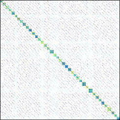
(a) Un-binned Hessian $597\times 597$

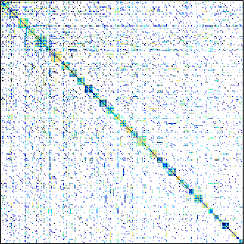
(b) Binned Hessian $321\times 321$

Figure 1: Two Hessians corresponding to the matrix specified in Equation (6). Plots generated using the cspy program [10] where darker pixel values correspond to larger magnitude.

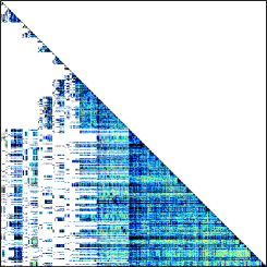
Figure 2: The lower triangular factor of the Hessian matrix shown in Figure 1(a) after the matrix is reordered by MATLAB to reduce fill-in. High fill-in mean sparse direct solvers will not be efficient.

We now show that once $N_{bin}$, the number of bins, is sufficiently large, the effects of binning on spectral properties of $X$ are little. Figure 3 shows the condition numbers of ${A}^{\dagger}X$ and relative Frobenius norm differences $\left|\left|{X}^{\dagger}-{A}^{\dagger}\right|\right|_{F}/\left|\left|{A}^{\dagger}\right|\right|_{F}$ for various number of bins. The lowest condition number is approximately 8.37, which is very close to the ‘exact’ answer 4.73 obtained without binning in [1].

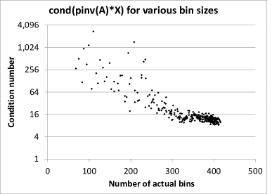
(a) $\text{cond}({A}^{\dagger}X)$

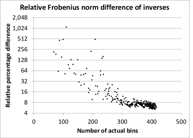
(b) $\left|\left|{X}^{\dagger}-{A}^{\dagger}\right|\right|_{F}/\left|\left|{A}^{\dagger}\right|\right|_{F}$

Figure 3: The figures shows that the spectral properties of of sparsified $X$ as well as the difference of inverses are not too perturbed even if binning is used with sufficient number of bins. The large differences for low number of bins is due to a few small singular values that are not approximated well.

Acknowledgements

This work was partially supported by the US Department of Energy SBIR Grant DE-FG02-08ER85154. The author thanks Travis M. Austin, Marian Brezina, Leszek Demkowicz, Ben Jamroz, Thomas A. Manteuffel, and John Ruge for many discussions.

References

- [1] C. Jhurani, Subspace-preserving sparsification of matrices with minimal perturbation to the near null-space. Part I: Basics, Submitted to Computers and Mathematics with Applications.
- [2] T. M. Austin, M. Brezina, B. Jamroz, C. Jhurani, T. A. Manteuffel, J. Ruge, Semi-automatic sparse preconditioners for high-order finite element methods on non-uniform meshes, Journal of Computational Physics 231 (14) (2012) 4694 – 4708.
- [3] T. Austin, M. Brezina, T. Manteuffel, J. Ruge, Efficient Preconditioned Solution Methods for Elliptic Partial Differential Equations, Bentham Science Publishers, 2011, Ch. Automatic Construction of Sparse Preconditioners for High-Order Finite Element Methods.
- [4] S. P. Boyd, L. Vandenberghe, Convex Optimization, Cambridge University Press, 2004.
- [5] Å. Björck, Numerical Methods for Least Squares Problems, SIAM, Philadelphia, 1996.
- [6] C. Jhurani, L. Demkowicz, Multiscale modeling using goal-oriented adaptivity and numerical homogenization: Part II. Algorithms for Moore-Penrose pseudoinverse, Computer Methods in Applied Mechanics and Engineering 213-216 (0) (2012) 418 – 426.
- [7] G. Quintana-Ort , X. Sun, C. Bischof, A BLAS-3 Version of the QR Factorization with Column Pivoting, SIAM Journal on Scientific Computing 19 (5) (1998) 1486–1494.
- [8] D. Braess, Finite Elements: Theory, fast solvers, and applications in solid mechanics, Cambridge University Press, 2007.
- [9] K. Martin, B. Hoffman, Mastering CMake: A Cross-Platform Build System, Kitware Inc, 2003.
- [10] T. A. Davis, www.cise.ufl.edu/research/sparse/SuiteSparse/.