Periodic Landau gauge and Quantum Hall effect in twisted bilayer graphene

Abstract

Energy versus magnetic field (Hofstadter butterfly diagram) in twisted bilayer graphene is studied theoretically. If we take the usual Landau gauge, we cannot take a finite periodicity even when the magnetic flux through a supercell is a rational number. We show that the periodic Landau gauge, which has the periodicity in one direction, makes it possible to obtain the Hofstadter butterfly diagram. Since a supercell can be large, magnetic flux through a supercell normalized by the flux quantum can be a fractional number with a small denominator, even when a magnetic field is not extremely strong. As a result, quantized Hall conductance can be a solution of the Diophantine equation which cannot be obtained by the approximation of the linearized energy dispersion near the Dirac points.

I Introduction

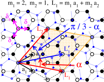
Figure 1: (color online). Twisted bilayer graphene with $(m_{1},m_{2})=(2,1)$. Large (small) open and filled circles are A and B sublattice in the first (second) layer, respectively. The second layer is rotated by $\pi/3-\alpha$. The orange area is the supercell.

Two dimensional electron systems are realized in graphene.Novoselov et al. (2004) Bilayer grapheneMcCann and Fal’ko (2006) and twisted bilayer grapheneShallcross et al. (2010) have been shown to have many interesting properties and been studied extensively. The quantum Hall effects in single layer grapheneNovoselov et al. (2005); Zhang et al. (2005) and bilayer graphene are well understood by the energy versus magnetic field, which is known as the Hofstadter butterfly diagram, in the tight binding models of honeycomb latticeHasegawa and Kohmoto (2006); Hatsugai et al. (2006); Dietl et al. (2008), and on Bernal-stacked bilayer grapheneNemec and Cuniberti (2007). The quantized value of the Hall conductance is obtained by the solution of the Diophantine equation.Thouless et al. (1982); Kohmoto (1985, 1989) Near half filled case, the quantum Hall conductance is given by a solution of the Diophantine equation Eq. (34) with $s_{r}=1$ ($s_{r}=2$) in single layer (bilayer) graphene.

Twisted bilayer graphene attracts much attention recently. When two layers are twisted in a commensurate way, a supercell becomes large with a moirè pattern Lopes dos Santos et al. (2007); Hass et al. (2008); Shallcross et al. (2008, 2010); Mele (2010) (see Fig. 1) and the velocity at the Dirac points is shown to become smaller when the rotation angle $\alpha$ is small.Trambly de Laissardière et al. (2010); Bistritzer and MacDonald (2011a)

Quantum Hall effect and the Hofstadter butterfly diagram in moirè superlattices have been observed experimentally in single layer graphene on hexagonal boron nitride (hBN)Ponomarenko et al. (2013) and Bernal-stacked bilayer graphene on hBN.Dean et al. (2013)

Electronic structure in twisted bilayer graphene in a uniform magnetic field has been studied only by taking the linearized energy dispersion near the Dirac pointsLee et al. (2011); Bistritzer and MacDonald (2011b); Moon and Koshino (2012) or by the Lanczos algorithm applied to large systems in real spaceWang et al. (2012). The whole lattice structure has not been taken into account when we take the linearized energy dispersion. Exact band structure is difficult to obtain by the Lanczos algorithm due to the finite-size effects and numerical errors.

When we use the usual Landau gauge in twisted bilayer graphene with long range hoppings, there are no periodicity in the phase factor of hoppings. In that case we cannot obtain the Hofstadter butterfly diagram. In this paper we show that we can recover the periodicity when a magnetic flux through a supercell is a rational number, if we use the periodic Landau gauge.As far as we know, a special choice of gauge was first used to study the system of the $4\times 4$ square lattice with periodic boundary conditions in the presence of the uniform magnetic flux $p/16$ with $p=1,2,3,\cdots$Poilblanc et al. (1990) (if a usual Landau gauge is used in that system, only magnetic flux $p/4$ is allowed). String gauge, which is obtained by adding the flux line with a flux quantum, has been introduced to study the periodic system in a magnetic field.Hatsugai et al. (1999) The periodic vector potential (equivalent to the periodic Landau gauge) has been introduced to study the Schrödinger equation with periodic potential in a uniform magnetic fieldTrellakis (2003), and it has been applied to study the tight binding model in Bernal stacked bilayer grapheneNemec and Cuniberti (2007). Another approach by using Fourier transform has been proposed for the periodic system in a magnetic field.Cai and Galli (2004) However, the periodic Landau gauge has not been used to study twisted bilayer graphene in a magnetic field. By virtue of the periodic Landau gauge we can calculate the energy spectrum in twisted bilayer graphene in a magnetic field in a similar way as in single layer grapheneHasegawa and Kohmoto (2006); Hatsugai et al. (2006); Dietl et al. (2008) or Bernal stacked bilayer grapheneNemec and Cuniberti (2007). We obtain very rich Hofstadter diagrams, which have not been obtained in previous studiesLee et al. (2011); Bistritzer and MacDonald (2011b); Moon and Koshino (2012); Wang et al. (2012). We find many energy gaps near half filled case, which are indexed by integers given by a solution of the Diophantine equation as $(s_{r},t_{r})=(2n_{0},2)$, $(2n_{0}\pm 2,0)$, $(2n_{0}\pm 2,2)$, $(2n_{0}\pm 4,2)$, $(2n_{0}\pm 6,2)$ $\cdots$, where $n_{0}$ is the number of the A site in the first layer in the supercell. The quantized value of the Hall conductance is obtained by $t_{r}$.

In Section II we define the twisted bilayer graphene with commensurate twisted angle. In Section III the tight binding model and the periodic Landau gauge are explained. In Section IV we show the Hofstadter butterfly diagram and study the quantized Hall conductances, which are obtained by the Diophantine equation. We give the summary in Section V. The detailed explanation of the periodic Landau gauge in the square lattice is given in Appendix A. The periodic Landau gauge in the twisted bilayer graphene is discussed in Appendix B.

II twisted bilayer graphene

In a unit cell in each layer there are two sites, A and B, which form triangular lattices respectively. We define unit vectors as

$$\mathbf{a}_{1}=a\left(\begin{array}[]{c}\frac{\sqrt{3}}{2}\\ -\frac{1}{2}\end{array}\right),$$ (1)

and

$$\mathbf{a}_{2}=R_{\pi/3}\mathbf{a}_{1}=a\left(\begin{array}[]{c}\frac{\sqrt{3}}{2}\\ \frac{1}{2}\end{array}\right),$$ (2)

where $a$ is the lattice constant and $R_{\pi/3}\mathbf{a}_{1}$ is the $\pi/3$ rotated vector of $\mathbf{a}_{1}$. Hereafter we take $a=1$ for simplicity. The reciprocal lattice vectors are given by

$$\mathbf{G}_{1} =2\pi\left(\begin{array}[]{c}\frac{1}{\sqrt{3}}\\ -1\end{array}\right),$$ (5)

$$\mathbf{G}_{2} =2\pi\left(\begin{array}[]{c}\frac{1}{\sqrt{3}}\\ 1\end{array}\right).$$ (8)

In the first layer, sites in the A sublattice are given by sets of two integers $(j_{1},j_{2})$ as

$$\mathbf{r}^{A}_{j_{1},j_{2}}=j_{1}\mathbf{a}_{1}+j_{2}\mathbf{a}_{2}.$$ (9)

Three vectors connecting nearest neighbor sites in the first layer are

$$\bm{\delta}_{a} =\left(\begin{array}[]{c}\frac{\sqrt{3}}{3}\\ 0\end{array}\right).$$ (12)

$$\bm{\delta}_{b} =\left(\begin{array}[]{c}-\frac{\sqrt{3}}{6}\\ \frac{1}{2}\end{array}\right),$$ (15)

$$\bm{\delta}_{c} =\left(\begin{array}[]{c}-\frac{\sqrt{3}}{6}\\ -\frac{1}{2}\end{array}\right).$$ (18)

Sites in the B sublattice in the first layer are given by

$$\mathbf{r}^{B}_{j_{1},j_{2}}=\mathbf{r}^{A}_{j_{1},j_{2}}+\bm{\delta}_{a}.$$ (19)

The AB (Bernal) stacking of bilayer graphene is obtained by rotating the second layer around one of the A site in the first layer by the angle $(2n+1)\pi/3$, where $n$ is an integer. In this case the A sublattice in the second layer is just above the A sublattice in the first layer, but the B sublattice in the second layer is on the center of the hexagon in the first layer. The same stacking is obtained by translating the second layer by $-\bm{\delta}_{a}$, $-\bm{\delta}_{b}$ or $-\bm{\delta}_{c}$. When the rotation angle is $2n\pi/3$, we obtain the AA stacking, i.e., all sites in the second layer are on the sites in the first layer. We obtain twisted bilayer graphene, when the rotation angle is neither $(2n+1)\pi/3$ nor $2n\pi/3$.

When twisted bilayer graphene has supercell with finite number of sites, it is called commensurate twisted bilayer graphene. We construct commensurate twisted bilayer graphene as follows; Since there is six-fold symmetry in twisted bilayer graphene, we can take a supercell as a diamond with the angle $\pi/3$ as shown in Fig. 1. We define unit vectors of superlattice with two integers $m_{1}$ and $m_{2}$ ($m_{1}\neq 0$, $m_{2}\neq 0$, and $|m_{1}|\neq|m_{2}|$):

$$\mathbf{L}_{1} =\mathbf{r}^{A}_{m_{1},m_{2}}=m_{1}\mathbf{a}_{1}+m_{2}\mathbf{a}_{2},$$ (20)

$$\mathbf{L}_{2} =R_{\pi/3}\mathbf{L}_{1}=\mathbf{r}^{A}_{-m_{2},(m_{1}+m_{2})}.$$ (21)

Twisted bilayer graphene with $(m_{1},m_{2})=(2,1)$ is shown in Fig. 1. Since

$$\mathbf{a}_{1}\cdot\mathbf{a}_{2}=\frac{1}{2},$$ (22)

we obtain

$$|\mathbf{L}_{1}|^{2}=|\mathbf{L}_{2}|^{2}=m_{1}^{2}+m_{2}^{2}+m_{1}m_{2}\equiv n_{0}.$$ (23)

The area of a supercell is given by

$$S=|\mathbf{L}_{1}||\mathbf{L}_{2}|\sin\frac{\pi}{3}=\frac{\sqrt{3}}{2}n_{0}.$$ (24)

There is another site in the supercell that has the same distance from the origin as $|\mathbf{L_{1}}|$, which we define $\mathbf{L}_{1}^{\prime}$ as shown in Fig. 1:

$$\mathbf{L}_{1}^{\prime}=\mathbf{r}_{m_{2},m_{1}}^{A}=m_{2}\mathbf{a}_{1}+m_{1}\mathbf{a}_{2}.$$ (25)

We define $\alpha$ by the angle between the vectors $\mathbf{L}_{1}^{\prime}$ and $\mathbf{L}_{1}$. Since

$$\mathbf{L}_{1}^{\prime}\cdot\mathbf{L}_{1}=\frac{1}{2}(m_{1}^{2}+4m_{1}m_{2}+m_{2}^{2}),$$ (26)

we obtain

$$\cos\alpha=\frac{\mathbf{L}_{1}^{\prime}\cdot\mathbf{L}_{1}}{|\mathbf{L}_{1}^{\prime}||\mathbf{L}_{1}|}=\frac{m_{1}^{2}+4m_{1}m_{2}+m_{2}^{2}}{2(m_{1}^{2}+m_{1}m_{2}+m_{2}^{2})}.$$ (27)

Then we obtain twisted bilayer graphene by rotating the second layer with the angle $\pi/3-\alpha$ to move the vector $\mathbf{L}_{1}^{\prime}$ into $\mathbf{L}_{2}$. We obtain another type of twisted bilayer graphene when we rotate the second layer by the angle $-\alpha$. In this paper we take the rotation angle $\pi/3-\alpha$ to obtain the Bernal stacking when $\alpha\to 0$.

The Bravais lattice of twisted bilayer graphene is the $-\alpha/2$-tilted two-dimensional triangular lattice with the primitive vectors $\mathbf{L}_{1}$ and $\mathbf{L}_{2}$. A supercell has $n_{0}$ sites in A and B sublattice in each layer, hence $4n_{0}$ sites.

III tight binding model and periodic Landau gauge

We consider tight binding models in a uniform magnetic field. Spin is not taken into account. When a magnetic field is applied, the hopping $t_{ij}$ between sites $\mathbf{r}_{i}$ and $\mathbf{r}_{j}$ ($\mathbf{r}_{i}$ and $\mathbf{r}_{j}$ are on the same layer or on different layers) has the factor $\exp(i\theta_{ij})$ with a phase $\theta_{ij}$ given by

$$\theta_{ij}=\frac{2\pi}{\phi_{0}}\int_{\mathbf{r}_{i}}^{\mathbf{r}_{j}}\mathbf{A}\cdot d\bm{\ell},$$ (28)

where $\mathbf{A}$ is a vector potential and

$$\phi_{0}=\frac{ch}{e},$$ (29)

is the flux quantum with charge $e$, the speed of light $c$ and the Planck constant $h$. The Hamiltonian is

$$\mathcal{H} =-\sum_{(i,j)}(e^{i\theta_{ij}}t_{ij}c^{\dagger}_{j}c_{i}+h.c.),$$ (30)

where $c^{\dagger}_{i}$ and $c_{i}$ are the creation and annihilation operators at site $i$, respectively. We take the approximationNakanishi and Ando (2001); Trambly de Laissardière et al. (2010); Moon and Koshino (2012),

$$t_{ij}=\left\{\begin{array}[]{l}t\exp\left(-\cfrac{d-|\bm{\delta_{a}}|}{\delta}\right)\\ \hskip 34.14322pt\mbox{ if sites $i$ and $j$ are on the same layer}\\ t_{12}\exp\left(-\cfrac{d-d_{0}}{\delta_{12}}\right)\\ \hskip 34.14322pt\mbox{ if sites $i$ and $j$ are on different layers}\end{array}\right.,$$ (31)

where $d=|\mathbf{r}_{i}-\mathbf{r}_{j}|$ is the distance between sites $i$ and $j$ and $d_{0}$ is the distance between layers. When we take $\delta\to 0$ and $t_{12}=0$, we obtain two independent layers of honeycomb lattice with only nearest-neighbor hoppings. When $t_{12}$, $\delta$ and $\delta_{12}$ are finite, we obtain twisted bilayer graphene with finite range hoppings. Interlayer hoppings are not restricted to the perpendicular direction.

The energy is independent of the sign of the interlayer hoppings $t_{12}$, since we obtain the same Hamiltonian by changing the sing of $t_{12}$, and the signs of $c_{i}^{\dagger}$ and $c_{i}$ in the second layer simultaneously.

Even if the flux per supercell is an integer times the flux quantum $\phi_{0}$, the phase factor $\theta_{ij}$ is not periodic with modulus $2\pi$, if we use the usual Landau gauge ($\mathbf{A}=Hx\hat{\mathbf{y}}$). For single layer graphene with only nearest-neighbor hoppings, we could take a special gaugeHasegawa and Kohmoto (2006); Hatsugai et al. (2006); Rhim and Park (2012), in which the phase factor appears only in the links for one of the three directions, $\bm{\delta}_{a}$, $\bm{\delta}_{b}$ or $\bm{\delta}_{c}$. However, such choice of gauge is not possible for twisted bilayer graphene.

In this paper we study the energy spectrum in the twisted bilayer graphene in magnetic field by using the periodic Landau gauge, which is essentially the same as the gauge used by Nemec and CunibertiNemec and Cuniberti (2007) to study the Bernal stacked bilayer graphene. We explain the periodic Landau gauge for the square lattice in Appendix A. The generalization to the non-square lattice is given in Appendix B.

When flux through a supercell is

$$\Phi=SH=\frac{p}{q}\phi_{0},$$ (32)

where $p$ and $q$ are mutually prime integers in twisted bilayer graphene with commensurate twisted angle (Eq.(27)), energy spectrum is obtained by the eigenvalues of $(4n_{0}q)\times(4n_{0}q)$ matrix, as in the case of the single layer graphene where it is obtained by the eigenvalues of $(2q)\times(2q)$ matrix.Hasegawa and Kohmoto (2006)

In Figs. 2, we plot the energy versus magnetic flux through a unit cell in single layer graphene with only nearest-neighbor hoppings. In Figs. 3, 4, and 5, we take parameters for the bilayer grapheneMoon and Koshino (2012) $t=2.7$ eV, $t_{12}=-0.48$ eV ($t_{12}/t=-0.18$), $|\bm{\delta}_{a}|=0.142$ nm, $d_{0}=0.335$ nm, and $\delta=\delta_{12}=0.0453$ nm ($\delta/|\bm{\delta}_{a}|=0.184$), and we plot the energy versus magnetic flux through a unit cell in each layer ($\phi=\Phi/n_{0}$) in twisted bilayer graphene.

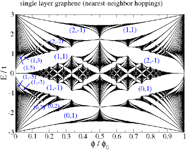
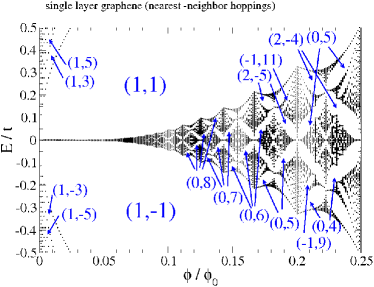
Figure 2: (color online). Energy spectrum in single layer graphene with only nearest-neighbor hoppings. Numbers in the figures are $(s_{r},t_{r})$. Quantized value of Hall conductance is given by $t_{r}$. See Eqs. (34) and (35).

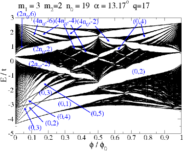
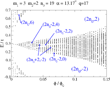
Figure 3: (color online). Energy spectrum in twisted bilayer graphene with $(m_{1},m_{2})=(3,2)$. Numbers in the figures are $(s_{r},t_{r})$. Quantized value of Hall conductance is given by $t_{r}$.

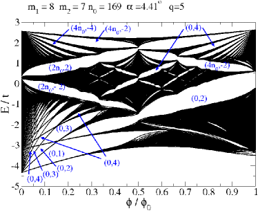
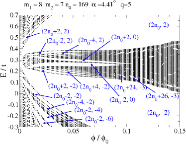
Figure 4: (color online). Energy spectrum in twisted bilayer graphene with $(m_{1},m_{2})=(8,7)$. Numbers in the figures are $(s_{r},t_{r})$. Quantized value of Hall conductance is given by $t_{r}$.

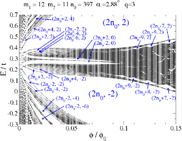
Figure 5: (color online). Energy spectrum in twisted bilayer graphene with $(m_{1},m_{2})=(12,11)$. Numbers in the figures are $(s_{r},t_{r})$. Quantized value of Hall conductance is given by $t_{r}$.

IV Diophantine equation

Consider the case

$$\frac{\Phi}{\phi_{0}}=\frac{p}{q},$$ (33)

where $\Phi$ is the flux through a supercell, $p$ and $q$ are integers. In square lattice and honeycomb lattice $\Phi=\phi$, and in twisted bilayer graphene $\Phi=n_{0}\phi$, where $\phi$ is the flux through a unit cell in each layer. When chemical potential is in the $r$th gap from the bottom, we have the Diophantine equationThouless et al. (1982); Kohmoto (1985, 1989); Sato et al. (2008)

$$r=qs_{r}+pt_{r},$$ (34)

which gives quantized Hall conductance by

$$\sigma_{xy}=\frac{e^{2}}{h}t_{r}.$$ (35)

If we take account of the spin and neglect the Zeeman energy, the Hall conductance is multiplied by $2$.

For the tight binding models with only nearest-neighbor hoppings in square lattice or honeycomb lattice, the flux quantum $\phi_{0}$ through a unit cell is equivalent to zero magnetic flux. As a result, the energy spectrum is periodic with respect to $\phi$ with a period $\phi_{0}$. Even when we consider the models with long range hoppings, the energy spectra are periodic function of $\phi$ with a period $2\phi_{0}$ or $6\phi_{0}$ in the square lattice or the honeycomb lattice, respectively. This is because the smallest areas enclosed by hoppings are $1/2$ and $1/6$ of the areas of a unit cell in the square lattice and the honeycomb lattice, respectively. See Fig. 6 for the honeycomb lattice. The energy spectrum is also periodic with respect to $\phi$ with a period $6\phi_{0}$ for Bernal stacked bilayer graphene. The situation is drastically changed in twisted bilayer graphene. When there are hoppings between layers in twisted bilayer graphene, projected areas enclosed by hoppings have irrational values as shown in the red triangles in Fig. 6. As a result the energies are not periodic in $\phi$.

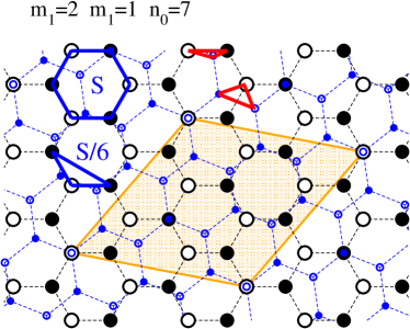
Figure 6: (color online). Twisted bilayer graphene. When there are only nearest-neighbor hoppings in each layer, an area enclosed by hoppings is $S$ (blue hexagon). When there are second-nearest-neighbor or third-nearest-neighbor hoppings in each layer, areas enclosed by hoppings are $S/6$ and its multiples (blue triangle). The hoppings between layers make the area enclosed by hoppings to be irrational number times $S$ (red triangles).

In single layer graphene, there are $2q$ band when flux through a supercell is $(p/q)\phi_{0}$. In Fig. 2, we show $(s_{r},t_{r})$ for several gaps for single layer grapheneHasegawa and Kohmoto (2006). Large gaps have indices $t_{r}=0$, $1$ , and $2$. The gaps, which are focused at the bottom of the band at $\phi\to 0$, have $s_{r}=0$, and $t_{r}=1,2,3,\cdots$. They correspond to the usual Landau levels. The gaps, which are focused at the top of the band at $\phi\to 0$, have $s_{r}=2$, and $t_{r}=-1,-2,-3,\cdots$. The gaps near half filling ($E\approx 0$) and $\phi\ll\phi_{0}$ have $s_{r}=1$ and $t_{r}=\pm 1,\pm 3,\pm 5,\cdots$, which have been observed in grapheneNovoselov et al. (2005); Zhang et al. (2005). For the finite $\phi$ the band near $E\approx 0$ becomes broadened gradually and many gaps can be seen in Fig. 2. Note that $\phi=\phi_{0}$ in a unit cell corresponds to $40,000$ T, which is not attainable in a present day laboratory.

In Figs. 3, 4, and 5, we plot the Hofstadter butterfly diagrams for twisted bilayer graphene with $(m_{1},m_{2})=(3,2)$, $(8,7)$ and $(12,11)$, respectively. Although energy gaps near the bottom have $s_{r}=0$ and $t_{r}=1,2,3,\cdots$, for all three cases as in single layer graphene, there are crossings of the bands near the bottom of the energy. For example, the gap indexed by $(0,2)$ vanishes at $\phi/\phi_{0}\approx 0.16$ and $E/t\approx-2.8$, at which band-crossing occurs. These crossings of bands can be understood by the independent Landau levels for the two local minimums of the energy in the absence of a magnetic field (see Fig. 7).

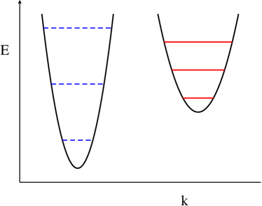
Figure 7: (color online). Schematic band structure near the bottom of the energy. There are two local minimums and nearly independent Landau Levels (dashed blue lines and solid red lines).

Near the top of the energy the large gaps are indexed by $(s_{r},t_{r})=(4n_{0},-2),(4n_{0},-4),(4n_{0},-6),\cdots$, which can be understood by the fact that there are $4n_{0}$ bands and nearly degenerate two local maxima of the energy in the absence of a magnetic field.

A very interesting feature is seen near half filling. Besides the large gaps of $(s_{r},t_{r})=(2n_{0},\pm 2)$, many new gaps become visible as $\alpha$ becomes small. For example, $(s_{r},t_{r})=(2n_{0}\pm 2,0),(2n_{0}\pm 2,\pm 2),(2n_{0}\pm 4,\pm 2),(2n_{0}\pm 6,\pm 2),\cdots$ are seen in the lower figures in Figs. 4 and 5. These new gaps are caused by a large supercell, which has $4n_{0}$ sites. Since Hall conductance is given by $t_{r}$, the band between the gaps with same $t_{r}$ ($(2n_{0},2)$ and $(2n_{0}-2,2)$, for example) does not contribute to the Hall conductance. Mathematically, that band is a Cantor set and consists of narrower bands and much smaller gaps. Each narrow band gives a finite Hall conductance and the total contribution vanishes.

V summary

We obtain the Hofstadter butterfly diagram for twisted bilayer graphene. The use of the periodic Landau gauge is crucial. Due to large number of sites ($4n_{0}$) in a supercell, a rich structure of the Hofstadter butterfly diagram appears, especially near half-filling and for small rotation angle $\alpha$. The gaps are indexed by two integers $s_{r}$ and $t_{r}$ (Eq. (34)). The Hall conductance is given by $\sigma_{xy}=(e^{2}/h)t_{r}$. While gaps with $s_{r}=0$, $1$ and $2$ are large in single layer graphene, many gaps with $s_{r}=2n_{0},2n_{0}\pm 2,2n_{0}\pm 4,\cdots$ become large as $\alpha$ becomes small. Since a supercell becomes large as $\alpha\to 0$, flux per supercell versus the flux quantum ($\Phi/\phi_{0}=p/q$) can be a rational number with a small denominator $q$ in not an extremely strong magnetic field. For $m_{1}=12$ and $m_{2}=11$, we obtain $n_{0}=392$. In that case $100$ T corresponds to $\Phi/\phi_{0}\approx 1$, which may be attained in experiment.

Near half-filling, there are many narrow bands, which do not contribute to the Hall conductance when they are completely filled. For example, the bands between the gaps with $(s_{r},t_{r})=(2n_{0}+2,2)$, $(2n_{0},2)$, $(2n_{0}-2,2)$, $(2n_{0}-4,2)$, etc. at $E/t\approx 0.3\sim 0.4$ in the lower figure in Fig. 5 do not change the quantized value of the Hall conductance $t_{r}=2$. Similarly the band between the gaps with $(s_{r},t_{r})=(2n_{0}+2,0)$ and $(2n_{0}-2,0)$ at $E/t\approx 0.3$ in the lower figure in Fig. 5 does not change the quantized value of the Hall conductance $t_{r}=0$. The narrow bands, in fact, consist of even narrower bands, since an energy spectrum is a Cantor set. One can expect other value of $t_{r}$ in the narrower band. It may be possible to observe these phenomena experimentally.

Appendix A periodic Landau gauge in square lattice

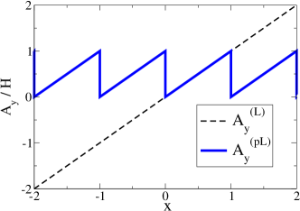
Figure 8: (color online). The $y$ component of vector potentials for Landau gauge ($A^{(L)}_{y}$, dashed line) and periodic Landau gauge ($A^{(pL)}_{y}$, thick blue line) for the square lattice.

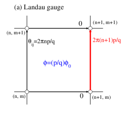
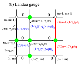
Figure 9: (color online). (a) The numbers beside the arrows are the phases in the usual Landau gauge for the square lattice with flux $(p/q)\phi_{0}$ in a unit cell. The system is periodic in the $x$ direction with period $q$. (b) Sites are added at $(n+\gamma_{1},m)$, $(n,m+\gamma_{2})$, and $(n+\gamma_{1},m+\gamma_{2})$, where $n$ and $m$ are integers, $0<\gamma_{1}<1$ and $0<\gamma_{2}<1$ (filled green circles). Blue letters are flux in rectangles. The system is periodic only when $\gamma_{2}$ is a rational number. (c) The phases (beside arrows) and the flux through rectangles (blue letters) in the periodic Landau gauge. The system is periodic in the $x$ direction with period $1$ and in the $y$ direction with period $q$.

We explain the periodic Landau gauge in the square lattice. A vector potential $\mathbf{A}$ gives a magnetic field

$$\mathbf{H}=\nabla\times\mathbf{A}.$$ (36)

For a uniform magnetic field $\mathbf{H}=H\hat{\mathbf{z}}$, one can take the Landau gauge

$$\mathbf{A}^{(L)}=Hx\hat{\mathbf{y}},$$ (37)

where $\hat{\mathbf{y}}$ is the unit vector along the $y$ direction and there is no dependence on $y$. In this case, however, $A^{(L)}_{y}$ is not periodic in the $x$ direction as shown by the dashed line in Fig. 8. We can obtain other vector potential by gauge transformation, i.e., adding $\nabla\chi(\mathbf{r})$ to $\mathbf{A}$. It is crucial to have periodicity in a gauge of twisted bilayer graphene. We take

$$\chi(\mathbf{r})=-H\lfloor x\rfloor y,$$ (38)

and so,

$$\mathbf{A}^{(pL)} =H\left(x\hat{\mathbf{y}}-\nabla(\lfloor x\rfloor y)\right)$$

$$=H\left((x-\lfloor x\rfloor)\hat{\mathbf{y}}-y\sum_{n=-\infty}^{\infty}\delta(x-n+\epsilon)\hat{\mathbf{x}}\right),$$ (39)

where $\epsilon$ is an infinitesimal and $\lfloor x\rfloor$ is the floor function (largest integer not greater than $x$), i.e. $x-\lfloor x\rfloor$ is the fractional part of $x$. In this gauge, which we call the periodic Landau gauge, $A^{(pL)}_{y}$ is periodic with respect to $x$ with period 1, as shown in Fig. 8. In order to make $A^{(pL)}_{y}$ be periodic in the $y$ direction $A^{(pL)}_{y}$ is a discontinuous function of $x$ as shown in Fig. 8 and $A^{(pL)}_{x}$ is the sum of delta functions. These singular functions do not cause any problems. We have no ambiguity in the phase factor $\theta_{ij}$, since we have added the infinitesimal $\epsilon$Trellakis (2003); Nemec and Cuniberti (2007).

Note that $A^{(pL)}_{x}$ depends on $y$ and it is not periodic in the $y$ direction. However, the dependence of $y$ in $\mathbf{A}^{(pL)}$ appears always with the delta function, so $\exp(i\theta_{ij})$ is periodic in the $y$ direction, as we show below.

The difference of the usual Landau gauge and the periodic Landau gauge is seen in Fig. 9 in which a uniform magnetic field with $(p/q)\phi_{0}$ through a unit cell is applied to square lattice. If we take the usual Landau gauge, the phase factor is zero except vertical links as shown in Fig. 9 (a). The phase factor for the vertical links at $x=n$ is $\theta_{ij}=2\pi np/q$. The periodicity in the $x$ direction is $q$ times larger than the periodicity in the absence of a magnetic field. However, if there are other sites in a unit cell, the periodicity of the system is changed (this is the case in twisted bilayer graphene, where there are $4n_{0}$ sites in the supercell (see Figs. 1 and 6)). In order to demonstrate it in the square lattice, we add sites at $(n+\gamma_{1},m)$, $(n,m+\gamma_{2})$, and at $(n+\gamma_{1},m+\gamma_{2})$, where $n$ and $m$ are integers, $0<\gamma_{1}<1$ and $0<\gamma_{2}<1$, as shown by the filled green circles in Fig. 9(b). The phase factors for the links connecting neighbor sites are shown in Fig. 9(b). The phase factor for the vertical link between $\mathbf{r}_{i}=(n,m)$ and $\mathbf{r}_{j}=(n,m+\gamma_{2})$ is $\theta_{ij}=2\pi n\gamma_{2}p/q$. If $\gamma_{2}$ is an irrational number, $\exp(i\theta_{ij})$ cannot be periodic with respect to $x$.

The periodicity is recovered by taking the periodic Landau gauge (Eq. (39)). The periodicity is 1 in the $x$ direction, since $\mathbf{A}^{(pL)}$ is periodic in the $x$ direction. The delta functions in Eq. (39) make the nonzero phases for the horizontal links as shown by thick red horizontal arrows in Fig, 9(c). The magnetic flux through each small rectangles is obtained by the sum of the surrounding phases $\theta_{ij}$ and it is proportional to the area. The phase factor for the horizontal link between $\mathbf{r}_{i}=(n+\gamma_{1},m)$ and $\mathbf{r}_{j}=(n+1,m)$ is $\theta_{ij}=-2\pi mp/q$, which does not depend on $\gamma_{1}$. The periodicity in the $y$ direction is $q$ times larger than that without magnetic field in the periodic Landau gauge.

Appendix B periodic Landau gauge in non-square lattice

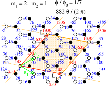
Figure 10: (color online). The first layer of twisted bilayer graphene with $(m_{1},m_{2})=(2,1)$ ($n_{0}=7$). The numbers on the links between the nearest neighbor sites show the phase $\theta_{ij}$ in the first layer in units of $2\pi/(18n_{0}^{2})=2\pi/882$ when the flux per supercell is $\phi_{0}$, i.e. the flux per unit hexagon is $\phi_{0}/n_{0}$ (We obtain $(4-(-35)+424-34-(-155)-148)\times 2\pi/882=2\pi/7$, for example). We take the periodic Landau gauge (Eq. (48)). The contribution from the delta function in Eq. (48) is finite for the red numbers, while it is zero for the blue numbers.

The periodic Landau gauge discussed in Appendix A is generalized to non-square two-dimensional lattices, which has primitive vectors of the supercell $\mathbf{L}_{1}$ and $\mathbf{L_{2}}$, which are not orthogonal. The reciprocal lattice vectors are

$$\mathbf{F}_{1} =2\pi\frac{\mathbf{L}_{2}\times\hat{\mathbf{z}}}{(\mathbf{L}_{1}\times\mathbf{L}_{2})\cdot\hat{\mathbf{z}}},$$ (40)

and

$$\mathbf{F}_{2} =2\pi\frac{\hat{\mathbf{z}}\times\mathbf{L}_{1}}{(\mathbf{L}_{1}\times\mathbf{L}_{2})\cdot\hat{\mathbf{z}}}.$$ (41)

We define oblique coordinate system $(\xi_{1},\xi_{2})$ by

$$\mathbf{r}=\left(\begin{array}[]{c}x\\ y\end{array}\right)=\xi_{1}\mathbf{L}_{1}+\xi_{2}\mathbf{L}_{2},$$ (42)

where $x$ and $y$ are the coordinates in a orthogonal system. For twisted bilayer graphene we have

$$\xi_{1} =\frac{1}{n_{0}}\left(\frac{\sqrt{3}}{3}(m_{1}+2m_{2})x-m_{1}y\right),$$ (43)

$$\xi_{2} =\frac{1}{n_{0}}\left(\frac{\sqrt{3}}{3}(m_{1}-m_{2})x+(m_{1}+m_{2})y\right).$$ (44)

The reciprocal vectors are

$$\mathbf{F}_{1} =\frac{m_{1}+m_{2}}{n_{0}}\mathbf{G}_{1}+\frac{m_{2}}{n_{0}}\mathbf{G}_{2},$$ (45)

and

$$\mathbf{F}_{2} =\frac{-m_{2}}{n_{0}}\mathbf{G}_{1}+\frac{m_{1}}{n_{0}}\mathbf{G}_{2}.$$ (46)

The Landau gauge for the oblique coordinate system is

$$\mathbf{A}^{(L,nsq)}=\frac{SH}{2\pi}\xi_{1}\mathbf{F}_{2},$$ (47)

which is a generalization of Eq. (37) to the non-square lattice. To make the vector potential periodic with respect to $\xi_{1}$, we take the periodic Landau gauge as

$$\mathbf{A}^{(pL,nsq)}= \frac{SH}{2\pi}\Bigl{(}(\xi_{1}-\lfloor\xi_{1}\rfloor)\mathbf{F}_{2}$$

$$-\xi_{2}\sum_{n=-\infty}^{\infty}\delta(\xi_{1}-n+\epsilon)\mathbf{F}_{1}\Bigr{)}.$$ (48)

In Fig. 10 we show an example of $\theta_{ij}$ between the nearest neighbor sites in the first layer for $m_{1}=2$, $m_{2}=1$ ($n_{0}=7$) and the flux through a supercell is $\phi_{0}$ ($p/q=1/1$). Note that the phase factor $\theta_{ij}$ crossing the line $\xi_{1}=n$ (red numbers in Fig. 10) is not periodic in the $\mathbf{L}_{2}$ direction but $\exp(i\theta_{ij})$ is periodic.

The advantage of taking the periodic Landau gauge is that the vector potential $\mathbf{A}$ is periodic in $\xi_{1}$ with period 1. This ensures the periodicity of the system in $\mathbf{L}_{1}$ direction. The system has a periodicity in the $\mathbf{L}_{2}$ direction if the flux per supercell is an rational number times $\phi_{0}$.

If the flux per a supercell is a rational number $p/q$ with integers $p$ and $q$, i.e.

$$\Phi=n_{0}\phi=SH=\frac{p}{q}\phi_{0},$$ (49)

the phase factor $\theta_{ij}$ in Eq. (28) with the periodic Landau gauge (Eq. (48)) has the same value when $\mathbf{r}_{i}$ and $\mathbf{r}_{j}$ are translated by $\mathbf{L}_{1}$. It has also the same value when $\mathbf{r}_{i}$ and $\mathbf{r}_{j}$ are translated by $\mathbf{L}_{2}$ if the link connecting $\mathbf{r}_{i}$ and $\mathbf{r}_{j}$ does not cross the line $\xi_{1}=n$, where $n$ is an integer. If the link connecting $\mathbf{r}_{i}$ and $\mathbf{r}_{j}$ crosses the line $\xi_{1}=n$, $\theta_{ij}$ increases by $\pm 2\pi p/q$ when $\mathbf{r}_{i}$ and $\mathbf{r}_{j}$ are translated by $\mathbf{L}_{2}$ ($\pm$ depends on the sign of $\mathbf{F}_{1}\cdot d\bm{\ell}$). Therefore periodicity must be $q$ times larger in the $\mathbf{L}_{2}$ direction.

References

- Novoselov et al. (2004) K. S. Novoselov, A. K. Geim, S. V. Morozov, D. Jaing, Y. Zhang, S. V. Dubonos, I. V. Grigorieva, and A. A. Firsov, Science 306, 666 (2004).
- McCann and Fal’ko (2006) E. McCann and V. I. Fal’ko, Phys. Rev. Lett. 96, 086805 (2006).
- Shallcross et al. (2010) S. Shallcross, S. Sharma, E. Kandelaki, and O. A. Pankratov, Phys. Rev. B 81, 165105 (2010).
- Novoselov et al. (2005) K. S. Novoselov, A. K. Geim, S. V. Morozov, D. Jiang, M. I. Katsnelson, I. V. Grigorieva, S. V. Dubonos, and A. A. Firsov, Nature 438, 197 (2005).
- Zhang et al. (2005) Y. Zhang, Y.-W. Tan, H. L. Stormer, and P. Kim, Nature 438, 201 (2005).
- Hasegawa and Kohmoto (2006) Y. Hasegawa and M. Kohmoto, Phys. Rev. B 74, 155415 (2006).
- Hatsugai et al. (2006) Y. Hatsugai, T. Fukui, and H. Aoki, Phys. Rev. B 74, 205414 (2006).
- Dietl et al. (2008) P. Dietl, F. Piéchon, and G. Montambaux, Phys. Rev. Lett. 100, 236405 (2008).
- Nemec and Cuniberti (2007) N. Nemec and G. Cuniberti, Phys. Rev. B 75, 201404 (2007).
- Thouless et al. (1982) D. J. Thouless, M. Kohmoto, M. P. Nightingale, and M. den Nijs, Phys. Rev. Lett. 49, 405 (1982).
- Kohmoto (1985) M. Kohmoto, Annals of Physics 160, 343 (1985).
- Kohmoto (1989) M. Kohmoto, Phys. Rev. B 39, 11943 (1989).
- Lopes dos Santos et al. (2007) J. M. B. Lopes dos Santos, N. M. R. Peres, and A. H. Castro Neto, Phys. Rev. Lett. 99, 256802 (2007).
- Hass et al. (2008) J. Hass, F. Varchon, J. E. Millán-Otoya, M. Sprinkle, N. Sharma, W. A. de Heer, C. Berger, P. N. First, L. Magaud, and E. H. Conrad, Phys. Rev. Lett. 100, 125504 (2008).
- Shallcross et al. (2008) S. Shallcross, S. Sharma, and O. A. Pankratov, Phys. Rev. Lett. 101, 056803 (2008).
- Mele (2010) E. J. Mele, Phys. Rev. B 81, 161405 (2010).
- Trambly de Laissardière et al. (2010) G. Trambly de Laissardière, D. Mayou, and L. Magaud, Nano Letters 10, 804 (2010).
- Bistritzer and MacDonald (2011a) R. Bistritzer and A. H. MacDonald, Proceedings of the National Academy of Sciences 108, 12233 (2011a), http://www.pnas.org/content/108/30/12233.full.pdf+html .
- Ponomarenko et al. (2013) L. A. Ponomarenko, R. V. Gorbachev, G. L. Yu, D. C. Elias, R. Jalil, A. A. Patel, A. Mishchenko, A. S. Mayorov, C. R. Woods, J. R. Wallbank, M. Mucha-Kruczynski, B. A. Piot, M. Potemski, I. V. Grigorieva, K. S. Novoselov, F. Guinea, V. I. Fal’ko, and A. K. Geim, Nature (London) 497, 594 (2013).
- Dean et al. (2013) C. R. Dean, L. Wang, P. Maher, C. Forsythe, F. G. andY. Gao, J. Katoch, M. Ishigami, P. Moon, M. Koshino, T. Taniguchi, K. Watanabe, K. L. Shepard, J. Hone, and P. Kim, Nature (London) 497, 598 (2013).
- Lee et al. (2011) D. S. Lee, C. Riedl, T. Beringer, A. H. Castro Neto, K. von Klitzing, U. Starke, and J. H. Smet, Phys. Rev. Lett. 107, 216602 (2011).
- Bistritzer and MacDonald (2011b) R. Bistritzer and A. H. MacDonald, Phys. Rev. B 84, 035440 (2011b).
- Moon and Koshino (2012) P. Moon and M. Koshino, Phys. Rev. B 85, 195458 (2012).
- Wang et al. (2012) Z. F. Wang, F. Liu, and M. Y. Chou, Nano Letters 12, 3833 (2012).
- Poilblanc et al. (1990) D. Poilblanc, Y. Hasegawa, and T. M. Rice, Phys. Rev. B 41, 1949 (1990).
- Hatsugai et al. (1999) Y. Hatsugai, K. Ishibashi, and Y. Morita, Phys. Rev. Lett. 83, 2246 (1999).
- Trellakis (2003) A. Trellakis, Phys. Rev. Lett. 91, 056405 (2003).
- Cai and Galli (2004) W. Cai and G. Galli, Phys. Rev. Lett. 92, 186402 (2004).
- Nakanishi and Ando (2001) T. Nakanishi and T. Ando, Journal of the Physical Society of Japan 70, 1647 (2001).
- Rhim and Park (2012) J.-W. Rhim and K. Park, Phys. Rev. B 86, 235411 (2012).
- Sato et al. (2008) M. Sato, D. Tobe, and M. Kohmoto, Phys. Rev. B 78, 235322 (2008).