Batched Kronecker product for 2-D matrices and 3-D arrays on NVIDIA GPUs

Abstract

We describe an interface and an implementation for performing Kronecker product actions on NVIDIA GPUs for multiple small 2-D matrices and 3-D arrays processed in parallel as a batch. This method is suited to cases where the Kronecker product component matrices are identical but the operands in a matrix-free application vary in the batch. Any batched GEMM (General Matrix Multiply) implementation, for example ours [1] or the one in cuBLAS [2], can also be used for performing batched Kronecker products on GPUs. However, the specialized implementation presented here is faster and uses less memory. Partly this is because a simple GEMM based approach would require extra copies to and from main memory. We focus on matrix sizes less than or equal to 16, since these are the typical polynomial degrees in Finite Elements, but the implementation can be easily extended for other sizes. We obtain 143 and 285 GFlop/s for single precision real when processing matrices of size 10 and 16, respectively on NVIDIA Tesla K20c using CUDA 5.0. The corresponding speeds for 3-D array Kronecker products are 126 and 268 GFlop/s, respectively. Double precision is easily supported using the C++ template mechanism.

1 Introduction

The Kronecker product is an important mathematical concept as well as a practical tool in multiple applications [3]. It is useful where either the domain or range of a linear operator or the space of unknowns is a “vector space” of matrices. It is commonplace for operator evaluation in high-order finite elements [4, 5], control theory [6], and when tensor-like decomposition is possible for different “directions” [7, 5].

Dense Kronecker product action has an additional advantage of possessing high arithmetic intensity just like the General Matrix Multiply (GEMM) routine in BLAS [8]. This is important on CPUs as well as GPUs [9]. In fact, matrix-free action of a Kronecker product can also be cast as a sequence of GEMM operations. Thus, modern computational hardware can achieve high performance in computing Kronecker product action. This makes it important to recognize if a computation can be cast in terms of Kronecker products and utilize it just like GEMM.

Our goal and contribution is to obtain high performance of Kronecker product action, possibly even higher than GEMM. We emphasize that we never form the explicit product matrix since it is rarely required. In our case, the sizes are small (less than or equal to 16) and the matrices are square but the method can be easily implemented for rectangular cases and for larger sizes. Such sizes correspond to the polynomial degrees and quadrature used in high-order finite elements [10, 4, 11, 12, 13]. However, we are unaware of any previous work done on GPUs. Part of the reason why this is so can be attributed to a lack of very high performance GEMM for batches of small matrices, a deficiency that we addressed in [1]. NVIDIA’s cuBLAS library also contains a batched GEMM implementation [2], which is different than ours.

If high-performance GEMM for small matrices is available, then one might deduce that fast Kronecker product action is a solved problem. This reasoning is not entirely correct though. We will show that the performance of even a fast GEMM implementation is less than a specialized Kronecker product action. This can be due to two separate reasons. In the first case, some components of the Kronecker product do not change in the batch and a general GEMM based approach cannot fully take advantage of this. In the second case, the domain and range of the action are not (2-D) matrices but 3-D arrays and more data movement to and from GPU memory reduces the overall speed. Both 2-D and 3-D cases arise in practice [4].

In order to achieve our goal, we also design a general BLAS-like function interface for Kronecker product action. Neither BLAS nor LAPACK implement such an interface [8], although it is possible to integrate it easily and would fit perfectly in their design philosophy. We design interfaces for matrices as well as 3-D arrays.

We obtain 143 and 285 GFlop/s for single precision real when processing matrices of size 10 and 16, respectively on NVIDIA Tesla K20c using CUDA 5.0. The corresponding speeds for 3-D array Kronecker products are 126 and 268 GFlop/s, respectively. This performance is appreciably better than current batched GEMM performance [1] and justifies the effort required for a specialized implementation.

Here is an outline of the paper. In Section 2 we describe our notation for Kronecker products for 2-D as well as 3-D batched inputs. Section 3 shows a few function interfaces required for the implementation. We give an algorithmic overview of our implementation in Section 4. Finally, we present the performance of our implementation in Section 5 for various inputs and compare it to the performance of batched GEMM.

2 Kronecker product in 2-D and its generalizations

The standard way of defining Kronecker product is to define it as an output matrix that is computed from two arbitrary real or complex input matrices. We work in the complex field below for generality. Let $A\in\mathbb{C}^{m_{a}\times n_{a}}$ and $B\in\mathbb{C}^{m_{b}\times n_{b}}$. The Kronecker product of $A$ and $B$ is denoted by $A\otimes B$. It is an element of $\mathbb{C}^{m_{a}m_{b}\times n_{a}n_{b}}$, such that

$$A\otimes B=\begin{bmatrix}a_{11}B&\cdots&a_{1n_{a}}B\\ \vdots&\ddots&\vdots\\ a_{m_{a}1}B&\cdots&a_{m_{a}n_{a}}B\end{bmatrix}$$

decomposed block-wise. See [14, 15] for it properties and applications.

Rather than looking at the Kronecker product as a matrix, we, as is also common, think of it as a linear operator defined by its two input matrices $A$ and $B$. The domain of the operator $A\otimes B$ is $\mathbb{C}^{n_{b}\times n_{a}}$ and the range is $\mathbb{C}^{m_{b}\times m_{a}}$. The operator is defined by its action on a matrix $X\in\mathbb{C}^{n_{b}\times n_{a}}$. We have

$$(A\otimes B)\text{vec}(X)=\text{vec}(BXA^{T})$$

where “vec” is the vectorization operation that stacks columns of a matrix to form a vector, and $Y\in\mathbb{C}^{m_{b}\times m_{a}}$ is the output matrix. The superscript $T$ stand for transpose without any conjugation. One advantage of this is that forming the product matrix, which can be much larger, is not necessary for it to be applied. Another advantage is that computing matrix products using matrices $A$ and $B$ is faster. This is due to fewer floating point operations (by counting flops [3]) and because a BLAS level-3 operation GEMM is used in practice.

2.1 Generalizations to other dimensions

We now describe generalizations for the Kronecker product action so that the input and output need not be restricted to (2-D) matrices. The generalized mapping is from $n$-D arrays to $n$-D arrays for $n\geq 1$. However, to avoid complicating the notation, we work with $n\leq 3$ only. One application where the 3-D case arises as naturally as the 2-D case is when computing stiffness matrix action on tensor product finite elements [4].

First, let us unravel the matrix symbolism present in the 2-D case so that the summations are visible. We change our formulation a little so that the matrix $A$ is related to the first direction in $X$ and the matrix $B$ is related to the second direction in $X$. This will make the generalization natural when we proceed to 3-D. We now work with the operator $B\otimes A$ in the 2-D case, where $A$ and $B$ are of the same sizes as mentioned above. But now $X\in\mathbb{C}^{n_{a}\times n_{b}}$ and $Y=AXB^{T}\in\mathbb{C}^{m_{a}\times m_{b}}$. Expanding this, we get

$$Y_{ij}=\sum_{l}^{n_{a}}\sum_{m}^{n_{b}}A_{il}X_{lm}B_{jm}=\sum_{l}^{n_{a}}\sum_{m}^{n_{b}}A_{il}B_{jm}X_{lm}.$$

We generalize this summation to 1-D and 3-D, which means the input “$X$” and output “$Y$” will both be either 1-D or 3-D arrays. Extension to higher order products will be obvious.

In 1-D, we have a single summation as follows. Only matrix $A$ is needed.

$$Y_{i}=\sum_{l}^{n_{a}}A_{il}X_{l}$$

This case has a more familiar name. It is just a simple matrix-vector multiplication, $Y=AX$, where $Y$ and $X$ are vectors.

In 3-D, we have a triple summation as follows. This requires introduction of a matrix $C\in\mathbb{C}^{m_{c}\times n_{c}}$. We have $X\in\mathbb{C}^{n_{a}\times n_{b}\times n_{c}}$ and $Y\in\mathbb{C}^{m_{a}\times m_{b}\times m_{c}}$, where

$$Y_{ijk}=\sum_{l}^{n_{a}}\sum_{m}^{n_{b}}\sum_{n}^{n_{c}}A_{il}B_{jm}C_{kn}X_{lmn}.$$

It can be shown that the equation above is an expanded form of the equation below.

$$\text{vec}(Y)=(C\otimes B\otimes A)\text{vec}(X)$$

Here “vec” vectorizes 3-D arrays ($X$ and $Y$) similar to the 2-D column major order vectorization. The order of Kronecker operations in $C\otimes B\otimes A$ is immaterial and thus Kronecker product is associative.

We hide the vectorization operation notation below by denoting the 1-D operation by $Y=\mathcal{K}(A)(X)$, the 2-D operation by $Y=\mathcal{K}(A,B)(X)$, and the 3-D operation by $Y=\mathcal{K}(A,B,C)(X)$. This emphasizes that we are concerned with a linear operation on $n$-D arrays rather than computing a Kronecker product matrix.

2.2 Batched Kronecker products

We now describe the batched Kronecker product operation as it needs to be implemented in practice. Our choices are inspired by the BLAS/LAPACK interface design [8].

Let $op$ (standing for operation) refer to a mapping from matrices to matrices, such that $op(A)=A$ or $A^{T}$ or $A^{*}$ depending on an extra variable that can contain three values. The superscripts $T$ and $*$ stand for transpose and Hermitian-transpose, respectively. Fix real or complex matrices $A,B,$ and $C$. The matrices can be stored in single precision or double precision. Using the BLAS notation, $op(A)$ is $m_{a}\times n_{a}$, and $op(B)$ is $m_{b}\times n_{b}$, and $op(C)$ is $m_{c}\times n_{c}$.

Consider the 3-D case first. The inputs are $X^{p}$ for $p=1,2,\ldots,N$. Here $N$ stands for the batch size. Each $X$ is $n_{a}\times n_{b}\times n_{c}$. The outputs are $Y^{p}$, each being $m_{a}\times m_{b}\times m_{c}$, and are computed as follows.

$$Y^{p}\leftarrow\alpha\,\mathcal{K}(op(A),op(B),op(C))(X^{p})+\beta\,Y^{p}.$$

Here $\alpha$ and $\beta$ are given scalar values. Note that the matrices $A$, $B$, and $C$ do not change in the batch.

The 2-D case is almost the same, except that it is meaningful to have the $op$ operation apply on $X$ as well. We then have each $op(X)$ of size $n_{a}\times n_{b}$. The outputs are $Y^{p}$, each being $m_{a}\times m_{b}$. We have

$$Y^{p}\leftarrow\alpha\,\mathcal{K}(op(A),op(B))(op(X^{p}))+\beta\,Y^{p}.$$

The operations $op$ acting on $A$, $B$, and $C$ can be different, which leads to $3^{3}=27$ combinations in all for the complex case and $2^{3}=8$ combinations for the real case in 3-D. Of course, implementing all these cases will lead to code bloat, in which case one might avoid the full generalization and implement only the specific cases one is interested in. Another possibility is specific to our case. We have $A$, $B$, and $C$ as constants and thus the cost of transposing them once before using them for all matrices in the batch is relatively minor. This avoids all the $op$ related permutations (except those for $X$ in the 2-D case) in the implementation.

3 Batched function interface

We present BLAS-like function interfaces for 1-D, 2-D, and 3-D batched Kronecker products. Each input $X$ and each output $Y$ is stored in column-major order, just like the matrices $A,B,$ and $C$. Most of the naming convention below would be natural to BLAS and cuBLAS [2] users and is easily understood by reading the material presented earlier. Thus, we describe only what is new.

The letter T below stands for type and is for single or double precision real or complex. The two variables that need a little explanation are ldx2 and ldxp (and other similar ones for other matrices). Here ldx2 denotes the offset in number of elements between adjacent “planes” in the 3-D array $X$. It is the the number of elements that are stored in the half-open memory range corresponding to $[X_{lm1},X_{lm2})$, for example. Similarly ldxp denotes the offset between adjacent $X$ inputs. This also means that each input and output in a batch is stored at uniform offset from previous entity. These concepts and arguments for and against them were discussed in detail in [1]. Additionally, as discussed there, many code optimizations are possible using C++ templates (instead of duplicating code). To avoid losing focus, we do not repeat here how C++ templates are used.

Here is the interface for 1-D. This is almost as if we have implemented a batched GEMV operation. Note that having the option for $op$ on $X$ in 1-D is just an unnecessary complication. Hence we drop it.

void TKRON1(
    char transa,
    int ma, int na,
    int batch_count,
    const T* alpha,
    const T* A, int lda,
    const T* X, int ldp,
    const T* beta,
    T* Y, int ldp);

Here is the interface for 2-D.

void TKRON2(
    char transa, char transb, char transx,
    int ma, int na,
    int mb, int nb,
    int batch_count,
    const T* alpha,
    const T* A, int lda,
    const T* B, int ldb,
    const T* X, int ldx, int ldxp,
    const T* beta,
    T* Y, int ldy, int ldyp);

Finally, here is the interface for 3-D. Note that there is no transx input argument. We are not aware of an application that would require it. Besides, generalizing transpose for 3-D array cannot just be flipping two indices.

void TKRON3(
    char transa, char transb, char transc,
    int ma, int na,
    int mb, int nb,
    int mc, int nc,
    int batch_count,
    const T* alpha,
    const T* A, int lda,
    const T* B, int ldb,
    const T* C, int ldc,
    const T* X, int ldx, int ldx2, int ldxp,
    const T* beta,
    T* Y, int ldy, int ldy2, int ldyp);

We now give an interface for performing a specialized batched GEMM operation where the first matrix $A$ varies across the batch but the second matrix $B$ does not. This will be used for implementing TKRON3 (see Algorithm 1 ahead). Mathematically, our operation looks like this. Let $\alpha$ and $\beta$ be given scalars and $p=1,2,\ldots,N$. We want to compute

$$C^{p}\leftarrow\alpha\,op(A^{p})op(B)+\beta\,C^{p}$$ (1)

using the following interface. The suffix A specifies that the matrix $A$ varies in the batch and thus requires a parameter lda2.

void TGEMM_A(
    char transa, char transb,
    int m, int n, int k,
    const T* alpha,
    const T* A, int lda, int lda2,
    const T* B, int ldb,
    const T* beta,
    T* C, int ldc, int ldc2,
    int batch_count,
    int grid_size);

4 CUDA kernel implementation overview

Before describing a few details relevant to the CUDA based implementation, it is useful to see how the 3-D kernel TKRON3 can be implemented in terms of TKRON2 and the batched TGEMM_A shown earlier. To keep the discussion simpler, we show this for a non-batched operation, where only one $X$ is an input and only one $Y$ is the output. This is shown in Algorithm 1 using MATLAB notation.

Data: $A\in\mathbb{C}^{m_{a}\times n_{a}}$, $B\in\mathbb{C}^{m_{b}\times n_{b}}$, $C\in\mathbb{C}^{m_{c}\times n_{c}}$, $X\in\mathbb{C}^{n_{a}\times n_{b}\times n_{c}}$

Result: $Y\in\mathbb{C}^{m_{a}\times m_{b}\times m_{c}}$ where $\text{vec}(Y)=(C\otimes B\otimes A)\text{vec}(X)$

$Y\leftarrow\text{zeros}(m_{a},m_{b},m_{c})$

$tmp\leftarrow\text{zeros}(m_{a},m_{b},n_{c})$

% First kron(B,A) is appplied to matrices ‘in’ X.

% GEMM operations are used.

% This step corresponds to TKRON2.

for N = 1 $\to$ $n_{c}$ do

       $tmp(:,:,N)\leftarrow A*X(:,:,N)*B^{\prime}$

      

end for

% Then C is applied to compute slices of Y.

% GEMM operations are used again.

% reshape is an inexpensive MATLAB function.

% This step corresponds to TGEMM_A.

for J = 1 $\to$ $m_{b}$ do

       $Y(:,J,:)\leftarrow\text{reshape}(\text{reshape}(tmp(:,J,:),m_{a},n_{c})*C^{\prime},m_{a},1,m_{c})$

      

end for

Algorithm 1 A sequence of GEMM operations in MATLAB notation to compute Kronecker product action on a 3-D array. We implement this in CUDA for a batch of inputs in the TKRON3 interface.

We need two CUDA kernel implementations – one for the TKRON2 operation and the other one for TGEMM_A. Both kernel implementations resemble the TGEMM_multi_uniform_kernel implementation we discussed in [1]. Similar to that case, we have two distinct methods. The first one is for matrix sizes 1-16. The second can be used for matrices where the square matrix dimension can be factorized into a product of two nearly equal numbers. For example, 15 can be factorized as $3\times 5$ or $5\times 3$. The order is important. Experimentally, we saw that the second method is faster than the first one for sizes 15 and 16 and we use that to show the results. In both methods, each CUDA thread-block is used to process multiple matrices.

What is more important and different here is that all threads read the “constant” matrices in the batch and save them in the shared memory. This is an obvious enhancement that helps in getting a better performance compared to GEMM. Then, each CUDA block collectively and reads a new $X$ matrix and writes the results to a single $Y$ matrix.

Another issue is that (at least) our implementation of these interfaces requires temporary storage, or “work arrays” in the Fortran and LAPACK [8] parlance. However, we have not explicitly mentioned the details here. Our description of the implementation in Algorithm 1 does show how much temporary storage is needed in our implementation of TKRON3. We would like to stress here that although a work array based interface may look like a hassle and a relic when calling the function, it has practical and philosophical advantages even when dynamic allocation facilities are present. For example, the alternative of memory allocation (and deallocation) inside the routine might make it more expensive when large temporary storage is required. We noticed the detrimental effect on the speed when we did not use work arrays and called cudaMemalloc and cudaFree for large temporary storage. Dynamic allocation also changes the characteristics of a function. If the function could be made “pure”, that opportunity is lost. One also has to consider multi-threaded environments, error messages in case of memory errors, multiple devices, and other such responsibilities that are better handled at some level higher than a high-performance kernel call [16]. Work arrays provide the full generality with only a minor hassle, and one that can be easily hidden by writing a small wrapper if one desires.

5 Performance results

Our test hardware is the Tesla K20c GPU, which has a peak performance of 3.52 TFlop/s and 1.17 GFlop/s in singe and double precision, respectively. We work with the ECC (error-correcting code) mode turned off for all cases. Our code has been compiled with -arch=sm_35 -O2 options using the CUDA 5.0 toolkit. To stay within the global memory limit of the device for the largest matrix size 16, we use 100,000 inputs in the single-precision batch and half of that in the double-precision batch. We launch kernels on 5000 CUDA kernel thread-blocks. We have not used any transpose or conjugate-transpose operation in presenting the results, but the actual implementation allows for that. We have computed all the flop rates by using $4m^{3}$ and $6m^{4}$ as the number of flops required to perform Kronecker action in 2-D and 3-D, respectively. This holds for real matrices that are of size $m$. We will show results when $\alpha=1$ and $\beta=0$. Finally, the memory layout of matrices is such that all the leading dimension parameters are the smallest they can logically be for the given matrix sizes.

We show the speeds achievable for real single and double precision data types in Table 1. Both 2-D and 3-D results are shown there. In general, the 2-D results are slightly faster than the 3-D result. This is because the 3-D result requires two sets of kernel calls and the intermediate result is written to and read from the main memory. This is the $tmp$ array described in Algorithm 1.

We also compare the Kronecker product action speeds with the GEMM speeds we showed in [1] and the batched GEMM available in cuBLAS. The results are in Figure 1 and Figure 2 for single and double precision, respectively. The motivation is to show that the Kronecker product action can be appreciably faster than both our GEMM and the one in cuBLAS. Note that if GEMM were used to implement Kronecker product, then the effective speed would be even lower than that of GEMM because of redundant data movement. The figures show that the best possible speeds (without such a reduction) are much lower than our specialized implementation.

Size	Single-2	Single-3	Double-2	Double-3
1	1	1	1	1
2	7	6	6	5
3	21	17	19	15
4	47	38	38	32
5	80	63	63	51
6	86	67	78	61
7	122	100	109	90
8	177	146	156	135
9	138	122	89	88
10	143	126	108	103
11	171	151	134	128
12	169	153	145	137
13	166	149	151	137
14	162	150	153	141
15	202	187	160	154
16	285	268	152	169

Table 1: The GFlop/s rates when computing action of independent Kronecker products of various sizes and precisions using the TKRON2 and TKRON3 interfaces on an NVIDIA Tesla K20c. We use 100,000 inputs for single precision and 50,000 inputs for double precision (to stay within global memory limit of the device for the largest matrix size 16). The comparison with corresponding numbers for a GEMM baseline are made in Figure 1 and Figure 2.

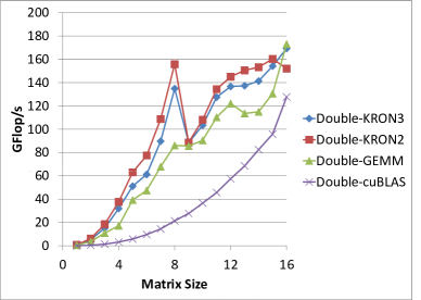
Figure 1: Performance obtained for single precision TKRON2 and TKRON3 when computing on 100,000 batched inputs with $\alpha=1$ and $\beta=0$ on an NVIDIA Tesla K20c. We show figures for our GEMM from [1] for comparison and the batched GEMM implemented in cuBLAS [2].

Figure 2: Performance obtained for double precision TKRON2 and TKRON3 when computing on 50,000 batched inputs with $\alpha=1$ and $\beta=0$ on an NVIDIA Tesla K20c. We show figures for our GEMM from [1] for comparison and the batched GEMM implemented in cuBLAS [2].

6 Discussion

We have described a BLAS-like interface for a batched Kronecker product routine generalized to 1-D, 2-D, and 3-D arrays. The implementation and results are for 2-D and 3-D only. Our implementation has assumed that the component matrices that form the Kronecker product are identical in the batch. This is obviously a design choice and based on our application requirement. If desired, one can similarly implement the computationally more expensive and general case where one or more of $A$, $B$, or $C$ matrix changes in the batch.

We have focused on NVIDIA GPUs and used CUDA throughout. However, the implementation does not use any special features that might not be available on other many-core hardware via OpenCL, for example. A new implementation will allow devices from other vendors with little or no change to the interface.

Acknowledgments

This work was partially supported by the US Department of Energy SBIR Grant DE-SC0004439. The author also thanks Paul Mullowney, Tech-X Corporation for supporting the work and providing GPU related help.

References

-
[1]
C. Jhurani, P. Mullowney,
A GEMM interface and implementation on NVIDIA GPUs for multiple small
matrices, Submitted.
URL {}{}}{www.ices.utexas.edu/$~$chetan/preprints/201%3-CJ-PM-GEMM.pdf}{cmtt} - [2] NVIDIA CUDA Basic Linear Algebra Subroutines (cuBLAS) library, https://developer.nvidia.com/cublas, accessed: Feb 21, 2013.
- [3] C.~F.~V. Loan, The ubiquitous Kronecker product, Journal of Computational and Applied Mathematics 123~(1--2) (2000) 85 -- 100.
- [4] M.~Deville, P.~Fischer, E.~Mund, High-Order Methods for Incompressible Fluid Flow, Cambridge University Press, 2002.
- [5] W.~Hackbusch, Tensor Spaces and Numerical Tensor Calculus, Springer--Verlag, Berlin, 2012.
- [6] A.~C. Antoulas, Approximation of Large-Scale Dynamical Systems, Cambridge University Press, 2005.
- [7] C.~V. Loan, N.~Pitsianis, Approximation with Kronecker Products, in: Linear Algebra for Large Scale and Real Time Applications, Kluwer Publications, 1993, pp. 293--314.
- [8] E.~Anderson, Z.~Bai, C.~Bischof, S.~Blackford, J.~Demmel, J.~Dongarra, J.~Du~Croz, A.~Greenbaum, S.~Hammarling, A.~McKenney, D.~Sorensen, LAPACK Users' Guide, 3rd Edition, SIAM, Philadelphia, PA, 1999.
- [9] R.~Nath, S.~Tomov, J.~Dongarra, An improved magma gemm for fermi graphics processing units, Int. J. High Perform. Comput. Appl. 24~(4) (2010) 511--515. doi:10.1177/1094342010385729.
- [10] G.~Karniadakis, S.~Sherwin, Spectral/hp Element Methods for CFD, Oxford University Press, USA, 1999.
- [11] L.~Demkowicz, Computing with hp-ADAPTIVE FINITE ELEMENTS: Volume I: One and Two Dimensional Elliptic and Maxwell Problems, Chapman & Hall/CRC Press, 2006.
- [12] L.~Demkowicz, W.~Rachowicz, D.~Pardo, M.~Paszynski, J.~Kurtz, A.~Zdunek, Computing with hp-ADAPTIVE FINITE ELEMENTS: Volume II Frontiers: Three Dimensional Elliptic and Maxwell Problems with Applications, Chapman & Hall/CRC Press, 2007.
- [13] P.~Šolín, K.~Segeth, I.~Doležel, Higher-order Finite Element Methods, Chapman & Hall/CRC, 2003.
- [14] N.~J. Higham, Accuracy and Stability of Numerical Algorithms, 2nd Edition, SIAM Books, Philadelphia, 2002.
- [15] R.~A. Horn, C.~R. Johnson, Matrix Analysis, Cambridge University Press, 1990.
- [16] J.~Lakos, Large-Scale C++ Software Design, Addison-Wesley professional computing series, Addison-Wesley Pub. Co, Reading, Mass, 1996.