Spectral imaging of the Central Molecular Zone in multiple 7-mm molecular lines

Abstract

We have imaged 24 spectral lines in the Central Molecular Zone (CMZ) around the Galactic Centre, in the range 42 to 50 GHz. The lines include emission from the CS, CH₃OH, HC₃N, SiO, HNCO, HOCO⁺, NH₂CHO, OCS⁺, CCS, C³⁴S, ¹³CS, ²⁹SiO, H¹³CCCN, HCC¹³CN and HC₅N molecules, and three hydrogen recombination lines. The area covered is Galactic longitude $-0.7$ to $1.8$ deg. and latitude $-0.3$ to $0.2$ deg., including the bright cores around Sgr A, Sgr B2, Sgr C and G1.6-0.025. This work used the 22-m Mopra radio telescope in Australia, obtaining $\sim 1.8$ km s^-1 spectral and $\sim 65$ arcsec spatial resolution. We present peak images from this study and conduct a principal component analysis on the integrated emission from the brightest 10 lines, to study similarities and differences in the line distribution. We examine the integrated line intensities and line ratios in selected apertures around the bright cores, as well as for the complete mapped region of the CMZ. We compare these 7-mm lines to the corresponding lines in the 3-mm band, for five molecules, to study the excitation. There is a variation in 3-mm to 7-mm line ratio across the CMZ, with relatively higher ratio in the centre around Sgr B2 and Sgr A. We find that the lines are sub-thermally excited, and from modelling with radex find that non-LTE conditions apply, with densities of order 10⁴ cm^-3.

1 Introduction

The Central Molecular Zone (CMZ) is the region within a few hundred parsecs of the Galactic Centre (Morris & Serabyn, 1996) with dense molecular gas, of total molecular mass a few times $10^{7}$ M_☉ (Ferrière, Gillard & Jean, Ferrière et al.2007). The CMZ is an unusual environment, with high molecular gas densities, large velocity dispersion and shears, high temperature, and rich chemistry: see Jones et al. (2012) and references therein.

Although there is on-going star formation in the CMZ, the star-formation rate (SFR) is an order of magnitude less than would be expected from such a large amount of molecular gas (Longmore et al., 2012) using common SFR scaling relations. Hence, studying the properties of the molecular medium in the CMZ is important in understanding the enviromental dependence of star formation, particularly the environments of the centres of galaxies.

We present here observations of the CMZ of 24 lines in the 7-mm band (including three hydrogen recombination lines), with resolution around 65 arcsec.

This is part of a larger project in which have also imaged the CMZ area in multiple lines in the 3-mm band, with resolution around 40 arcsec (Jones et al., 2012), and in the 12-mm band, with resolution around 120 arcsec, as part of the wider H₂O southern Galactic Plane Survey (HOPS, Walsh et al., 2008, 2011; Purcell et al., 2012). A further Mopra survey to image CO lines over a larger area of the CMZ is ongoing. We have also studied the smaller Sgr B2 sub-area of the CMZ with the molecular lines over the full 3-mm band from 82 to 114 GHz, and 7-mm band from 30 to 50 GHz, in Jones et al. (2008a) and Jones et al. (2011) respectively.

We use the distance to the Galactic Centre of 8.0 kpc (Reid et al., 2009), as per our previous papers, so 1 arcmin corresponds to 2.3 pc.

2 Observations and Data Reduction

The observations were made with the 22-m Mopra radio telescope, of the Australia Telescope National Facility (ATNF) using the UNSW MOPS digital filterbank. The Mopra MMIC (Monolithic Microwave Integrated Circuit) receiver has a bandwidth of 8 GHz, and the MOPS backend can cover the full 8-GHz range simultaneously in the broad band mode. This gives four 2.2-GHz sub-bands each with 8192 channels of 0.27 MHz. The lines in the CMZ are broad, so that these channels, corresponding to around 1.8 km s^-1, are quite adequate.

The Mopra receiver covers the range 30 to 50 GHz in the 7-mm band. We chose the tuning centred at 45.8 GHz, to cover the range 41.8 to 49.8 GHz, giving the spectral lines summarised in Table 1. This range was chosen to include the strong lines of CS near 49.0 GHz and SiO near 43.4 GHz, and several other bright lines as listed in the Table. This is also the densest part of the 30 to 50 GHz band for bright molecular lines, as seen by Jones et al. (2011) in Sgr B2.

Table 1: The lines imaged here in the 42 to 50 GHz range. The rest frequencies with a * indicate the frequency used for lines corresponding to multiple transitions, some also indicated as group (gp) in the transition list. The multiple components are, in general, blended due the large velocity widths in the CMZ area. The Mopra observations covered the whole 42 to 50 GHz range, so include weaker lines than are listed here, particularly in Sgr B2, see Jones et al. (2011).

Rough	Line ID	Transition	Exact
frequency	molecule		rest frequency
GHz	or atom		GHz
42.39	NH2CHO	2(0,2) – 1(0,1) gp	42.386070*
42.60	HC5N	16 – 15	42.602153
42.67	HCS+	1 – 0	42.674197
42.77	HOCO+	2(0,2) – 1(0,1)	42.7661975
42.82	SiO	1 – 0 v=2	42.820582
42.88	29SiO	1 – 0 v=0	42.879922
42.95	H	53 $\alpha$	42.951968
43.12	SiO	1 – 0 v=1	43.122079
43.42	SiO	1 – 0 v=0	43.423864
43.96	HNCO	2(0,2) – 1(0,1) gp	43.962998*
44.07	CH3OH	7(0,7) – 6(1,6) A++	44.069476
44.08	H13CCCN	5 – 4	44.084172
45.26	HC5N	17 – 16	45.264720
45.30	HC13CCN	5 – 4	45.297346
	HCC13CN	5 – 4	45.301707*
45.38	CCS	4,3 – 3,2	45.379029
45.45	H	52 $\alpha$	45.453719
45.49	HC3N	5 – 4 gp	45.490316*
46.25	13CS	1 – 0	46.247580
47.93	HC5N	18 – 17	47.927275
48.15	H	51 $\alpha$	48.153597
48.21	C34S	1 – 0	48.206946
48.37	CH3OH	1(0,1) – 0(0,0) A++	48.372467*
	CH3OH	1(0,1) – 0(0,0) E	48.376889
48.65	OCS	4 – 3	48.6516043
48.99	CS	1 – 0	48.990957

The area was observed with on-the-fly (OTF) mapping, in a similar way to that described in Jones et al. (2012), for the 3-mm CMZ observations.

The $10\times 10$ arcmin² OTF maps used a scan rate of 8 arcsec/second, with 24 arcsec line spacing, taking a little over an hour per block. We made pointing observations of SiO maser positions (AH Sco or VX Sgr), after every second map, to correct the pointing to within about 10 arcsec accuracy. The system temperature was calibrated with a continuous noise diode, but the 7-mm calibration system (unlike the 3-mm system) does not include ambient-temperature paddle scans, so some extra steps in processing were needed (see below) to correct for the atmospheric opacity. We included observations of line sources (Sgr B2, M17SW and G345.5+1.5) a few times each day, under different weather conditions and at different elevations, to check the calibration.

We used position switching for bandpass calibration with the off-source reference position observed before each 10 arcmin long source scan. The reference position (($\alpha,\delta)_{\rm J2000}=17^{\rm h}51^{\rm m}03\hbox to0.0pt{.\hss}$ ^s $6,-28^{\circ}22^{\prime}47^{\prime\prime}$, or $l=1.093$ deg., $b=-0.735$ deg.) was carefully selected to be relatively free of emission.

Each $10\times 10$ arcmin² block was observed twice, with Galactic latitude and longitude scan directions, to reduce scanning direction stripes and to improve the signal to noise. The overall $2.5\times 0.5$ deg² area was covered with a $15\times 3$ grid of blocks, separated by 10 arcmin steps, making 90 OTF observations required. In practice a few more OTF observations were used, including some areas with OTF maps stopped by weather or other problems and re-observed, or just areas re-observed in better weather. The area covered is between $-0.72$ to $1.80$ degrees Galactic longitude, and $-0.30$ to $0.22$ degrees Galactic latitude.

The observations were spread over two periods, in March 2010 and 2011. The conditions, in the southern hemisphere autumn, are warmer and wetter than the best winter observing periods. Although the blocks worst affected by poor weather were re-observed, the range of conditions during the different observations means that there are inevitably some blocks with greater noise level than others. In practice, we observed the central area including Sgr B2 and Sgr A in 2010, and the outer areas in 2011. The weather in 2011 Mar was not as good as in 2010, so that the system temperature was higher, and the noise level greater in the outer areas.

The OTF data were turned into FITS data cubes with the livedata and gridzilla packages, in a similar way to Jones et al. (2012). The bandpass correction used the off-source spectra, and a second order polynomial, and the gridding used a median filter.

The FITS cubes were then read into the miriad package for further processing and analysis. The velocity pixels were 0.27 MHz or $\sim$1.8 km s^-1, but to improve the signal-to-noise, and ensure the lines were Nyquist sampled, we applied a 3-point Hanning smoothing, leading to an effective resolution 0.54 MHz or $\sim$3.6 km s^-1. This is quite adequate spectral resoution for the broad lines in the CMZ, which are $>10$ km s^-1 wide, but for narrow spectral features, such as the maser lines, we use the data cubes in the original unsmoothed versions.

Small residual baseline offsets in the spectra were fitted and removed with a first order polynomial using the miriad task contsub.

The resolution of the Mopra beam varies between $1.14\pm 0.05$ arcmin at 43 GHz to $0.99\pm 0.04$ arcmin at 49 GHz (Urquhart et al., 2010). We take this as the beamsize inversely proportional to frequency, with $1.06$ arcmin or 64 arcsec at 46 GHz in the centre of the frequency range observed.

The main beam efficiency of Mopra varies between $0.53\pm 0.01$ at 43 GHz and $0.43\pm 0.01$ at 49 GHz, and the extended beam efficiency between $0.69\pm 0.01$ at 43 GHz and $0.56\pm 0.01$ at 49 GHz (Urquhart et al., 2010). Since we are largely concerned in this paper with the spatial and velocity structure, we have mostly left the intensities in the $T_{A}^{*}$ scale, without correction for the beam efficiency onto the $T_{MB}$ or $T_{XB}$ scales, except for some of the quantitative analysis sections.

A flux correction has been applied to the data cubes to take into account the atmospheric attenuation. The test spectra (of Sgr B2, M17SW and G345.5+1.5) showed a significant (a few times 10 %) decrease in flux associated with higher system temperatures. This was consistent with the effect expected with increased optical depth $\tau$ in the atmosphere, at lower elevation or higher humidity, increasing $T_{sys}$ with the addition of term $T_{amb}(1-\exp(-\tau))\sim\tau T_{amb}$ (where $T_{amb}\sim$ 290 K is the atmospheric temperature) and decreasing the flux by factor $\exp(-\tau)$. The system temperatures were measured in each of the 2 GHz sub-bands, across the overall 8 GHz range observed. When combined in the data cubes, averaged over the two passes in latitude and longitude scanning directions, the means were 84, 93, 106 and 126 K at around 43, 45, 47 and 49 GHz respectively, with RMS scatter 10, 11, 13 and 15 K respectively. However, due to outliers of data taken in poor weather, the full ranges were 68 – 190, 75 – 201, 85 – 219 and 101 – 231 K respectively. This provides a measure of the average optical depth $\tau$ as a function of position in the images, so allowing a correction for it to be applied. The flux correction factors applied to the cubes, as a function of position derived from the $T_{sys}$ images were $1.150\pm 0.044$, $1.180\pm 0.054$, $1.233\pm 0.068$ and $1.276\pm 0.087$ in the four sub-bands.

Table 2: Statistics of the data cubes. Both the RMS noise and peak brightness temperature are in $T_{A}^{*}$, after the calibration correction for atmospheric attenuation. The velocity range is that with line emission significantly above the noise level. We also quote the position and velocity of the peak pixel.

Line	Molecule	RMS	Velocity	Peak	Peak		Peak
Freq.	or atom ID	noise	range		lat.	long.	vel.
GHz		mK	km s-1	K	deg.	deg.	km s-1
42.39	NH2CHO	24	-5, 110	0.30	359.861	-0.082	8
42.60	HC5N	25	0, 100	0.33	0.687	-0.020	65
42.67	HCS+	26	-5, 85	0.24	0.675	-0.020	71
42.77	HOCO+	27	-5, 100	0.39	0.694	-0.020	62
42.82	SiO	26	-150, 200	3.22	0.550	-0.057	-25
42.88	29SiO	27	0, 85	0.17	0.836	-0.248	49
42.95	H 53 $\alpha$	29	35, 95	0.39	0.669	-0.037	64
43.12	SiO	28	-150, 200	2.74	0.550	-0.057	-26
43.42	SiO	40	-140, 205	1.48	359.893	-0.076	15
43.96	HNCO	38	-160, 185	2.68	1.649	-0.053	51
44.07	CH3OH	30	-60, 195	3.37	359.986	-0.069	47
44.08	H13CCCN	30	0, 90	0.22	0.698	-0.028	61
45.26	HC5N	30	0, 80	0.32	0.690	-0.026	63
45.30	HCC13CN	29	30, 105	0.25	0.675	-0.020	68
45.38	CCS	31	-5, 100	0.35	0.687	-0.020	70
45.45	H 52 $\alpha$	38	30, 90	0.42	0.669	-0.037	63
45.49	HC3N	37	-150, 200	2.67	359.981	-0.078	16
46.25	13CS	34	-15, 110	0.49	359.983	-0.071	52
47.93	HC5N	73	20, 80	0.37	0.675	-0.022	67
48.15	H 51 $\alpha$	67	40, 85	0.45	0.672	-0.035	58
48.21	C34S	59	-25, 140	0.81	359.982	-0.073	51
48.37	CH3OH	76	-160, 205	3.76	0.689	-0.024	71
48.65	OCS	55	-10, 105	0.72	0.691	-0.029	64
48.99	CS	75	-185, 210	3.51	359.984	-0.069	54

3 Results

3.1 Line data cubes

The frequencies and line identifications for the 24 strongest lines in the 41.8 to 49.8 GHz range, are listed in Table 1. These data are taken from the NIST online catalogue of lines known in the interstellar medium (Lovas & Dragoset, 2004) and the splatalogue compilation.

Some statistics of the data cubes are listed in Table 2. The RMS noise ranges from 24 to 76 mK, increasing with frequency across the 8 GHz range, with the highest noise for the 47.93 GHz HC₅N line, near the 47.8 GHz edge of the sub-band.

The velocity range listed in Table 2 indicates the range of significant emission (roughly greater than 3 $\sigma$) detected in the data cubes. The line widths in the CMZ are large, and there is a large velocity gradient across the CMZ (in the deep potential well of the Galactic Centre). Hence the integrated emission needs to summed over a large velocity range. This makes the integrated emission quite sensitive to low level baselevel offsets which are small in terms of brightness (e.g. of order 10 mK) but become significant (e.g. of order K km s^-1) when integrated over the velocity range (order 100 km s^-1). The 7-mm Mopra data here have better baselevel stability than the 3-mm data of Jones et al. (2012), due to the lesser sensitivity to the weather at lower frequencies. However, the baseline problems do provide a limit, along with the thermal noise, to the accuracy of the data.

These data cubes are publicly available in the CSIRO-ATNF archive, accessible from http://atoa.atnf.csiro.au/CMZ, together with the 3-mm and 12-mm data from the CMZ and Sgr B2.

3.2 Peak emission images

We show the 2-dimensional distribution of the line emission in Figs 1 to 4. We use peak images as these are are much more robust to the effect of low level baseline problems than the integrated emission images. They also better show fine spatial structure as they are less affected by multiple velocity components along the line of sight. The colour-scale or grey-scale displays start at the 3 $\sigma$ brightness level, so do not show noisy features in areas without significant line emission. However, low-level emission outside the areas highlighted in these plots, may be found to be significant when the data are integrated over larger areas than the beam, or smoothed in velocity.

There are some artifacts in some of these peak brightness images, notably areas at longitude 359.6 deg. with higher noise, giving maxima above the overall 3 $\sigma$ level.

The lines of CS, CH₃OH (at 48.37 GHz), HC₃N, SiO and HNCO are relatively strong and widespread (Fig. 1). The lines of HOCO⁺ (Fig. 1), NH₂CHO, OCS, HCS⁺, and CCS (Fig. 2) are weaker, and detected mostly in the Sgr B2 and Sgr A areas. The lines of HNCO, HOCO⁺ and OCS highlight the core of Sgr B2, and also the area of G1.6-0.025 (as discussed below in section 3.3).

The weaker isotopologues of CS, SiO and HC₃N, namely C³⁴S and ¹³CS in Fig. 2, ²⁹SiO, H¹³CCCN and HCC¹³CN (blended with HC¹³CCN) in Fig. 3, are also detected around the Sgr B2 and Sgr A areas. Note that the line of H¹³CCCN at 44.08 GHz (Fig. 3) is highly confused with the line of CH₃OH at 44.07 GHz (Fig. 4), so the peak image has additional strong CH₃OH maser peaks which overlap the frequency range. In principle, these isotopologues could be used to measure isotope ratios (C/¹³C, S/³⁴ and Si/²⁹) near the Galactic Centre. However, in practice, the low signal noise of the mapping data for these weaker isotopolgues means that they are only detected at the strong cores, where the strong isotopologues (CS, SiO and HC₃N) are optically thick, so the line ratios do not give the intrinsic isotope ratios.

The three lines of HC₅N (Fig. 3) show emission from Sgr B2, but the higher noise at the higher frequency means that the weaker emission at Sgr A and G1.6-0.025 detectable in the two lower frequency lines is lost in the noise for the last line.

The line of CH₃OH at 44.07 GHz (Fig. 4) has maser as well as thermal emission, so shows diffuse thermal emission around Sgr B2 and Sgr A, plus a number of maser spots distributed over a wider area of the CMZ.

The two maser lines of SiO in Fig. 4 are dominated by a strong maser peak (at $l=$ 0.550 deg., $b=$ -0.057 deg.) but also show a number of weaker maser spots. These are vibrationally excited lines, unlike the thermal v=0 line of SiO at 43.42 GHz, and so have a very different distribution to the latter.

The three hydrogen $\alpha$ radio recombination lines are at Sgr B2, which is where the thermal bremsstrahlung emission in the CMZ is strongest.

More details on the 7-mm line distributions in the area around Sgr B2 are given in Jones et al. (2011).

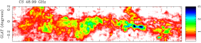
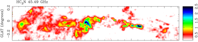
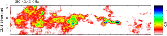
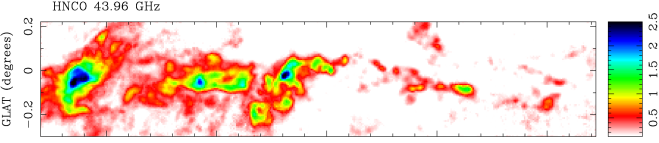
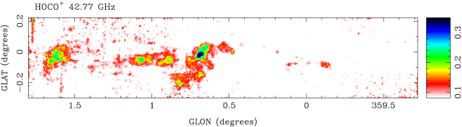
Figure 1: Peak brightness images for the lines of CS, CH₃OH, HC₃N, SiO, HNCO and HOCO⁺. These are the six lines we observed with the most widespread strong distribution. The grey-scale is peak brightness as $T_{A}^{*}$ in K here and in Figs 2 to 4.

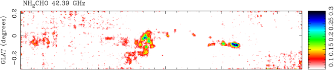
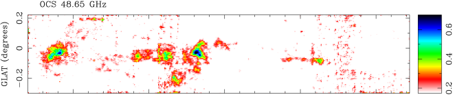
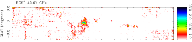
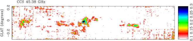
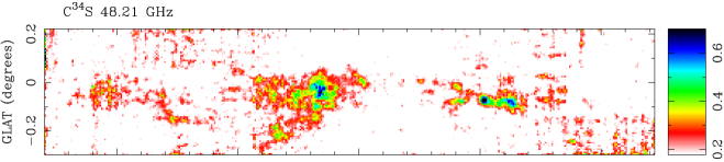
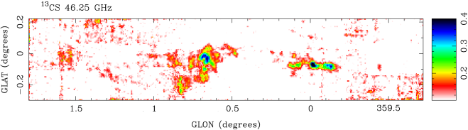
Figure 2: Peak brightness images for the lines of NH₂CHO, OCS, HCS⁺, CCS and the CS isotopologues C³⁴S and ¹³CS.

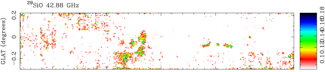
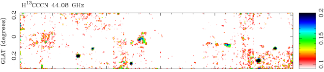
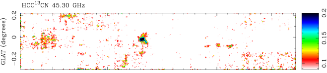
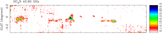
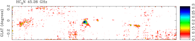
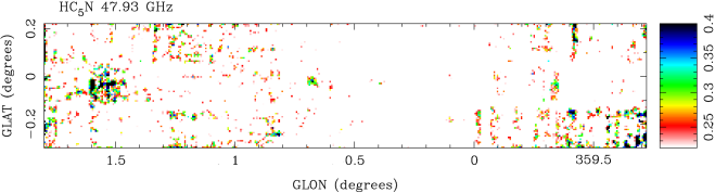
Figure 3: Peak brightness images for the lines of SiO isotopologue ²⁹SiO, HC₃N isotopologues H¹³CCCN and HCC¹³CN blended with HC¹³CCN, and three transitions of HC₅N. Note that the 44.08 GHz H¹³CCCN line is confused with the 44.07 GHz CH₃OH maser line (Fig. 4).

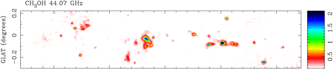
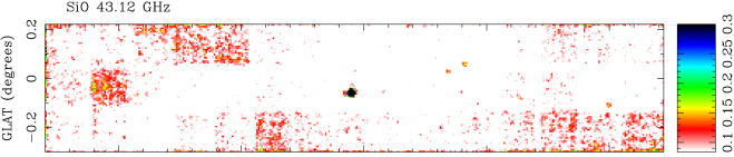
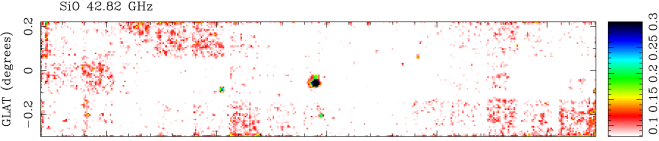
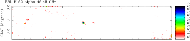
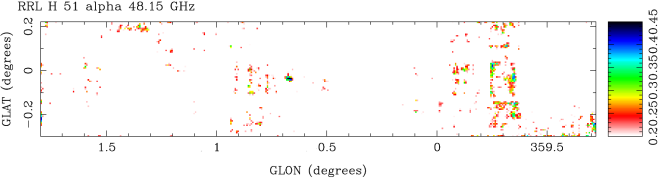
Figure 4: Peak brightness images for lines of CH₃OH in a maser transition, two maser transitions of SiO, and three hydrogen $\alpha$ recombination lines.

3.3 Principal Component Analysis

We can identify and quantify similarities and differences between the CMZ line emission here with Principal Component Analysis (PCA). This technique describes multi-dimensional data sets by linear combinations of the data that describe the largest variance (the most significant common feature) and successively smaller variances (the next most significant features). For integrated emission images here, PCA gives a series of images which contain the most significant features (Fig. 5) and a set of coefficients (Fig. 6) which describe how the individual line images are made up of linear combinations of these PCA images.

We have used this PCA technique on the Mopra line surveys of the CMZ at 3-mm (Jones et al., 2012), the Sgr B2 area at 3-mm and 7-mm (Jones et al., 2008b, 2011), and the G333 molecular cloud complex at 3-mm (Lo et al., 2009). These papers, and the references therein, give more details on the technique.

Since the PCA uses normalised versions of the input data sets, it does not work well with low signal to noise data, as the noisy data is scaled up, causing the result to be dominated by spurious features. Hence we use the ten strongest lines here (CS, CH₃OH (at 48.37 GHz), HC₃N, SiO, HNCO, HOCO⁺, NH₂CHO, OCS, C³⁴S and ¹³CS) out of the total of 24 lines. We consider the whole observed area, less a small cropping at the low sensitivity edges of the area. This is different to the PCA analysis of the CMZ 3-mm lines in Jones et al. (2012), where we applied an additional mask of low surface brightness areas, leaving only the stronger areas around Sgr B2 and Sgr A, because the 3-mm data were more badly affected by baseline ripples.

We use the versions of the integrated line emission (over the velocity ranges given in Table 2) with clipping below the 3 $\sigma$ level, as these are less affected by baseline ripple than the integrated emission without clipping. However, we have checked the PCA results from integrated emission, with and without this clipping, and find qualitatively similar results. Hence the PCA results are not too seriously affected by the small amount of missing flux caused by the 3 $\sigma$-level clipping.

The images of the three most significant components of the integrated emission are shown in Fig. 5. These three components describe 68.3, 11.5 and 7.3 percent respectively of the variance in the data. The normalised projection of the molecules onto the principal components are shown in Fig. 6 with successive pairs of components.

The first principal component (Fig. 5) shows emission common to all ten lines. As all of these lines are quite similar in overall morphology, it describes a large fraction (68.3 percent) of the variance. This behaviour is similar to that seen at 3-mm (Jones et al., 2012), where the first component displays an averaged intensity image of all the molecular lines (albeit with a factor two better resolution).

The second principal component (Figs. 5 and 6) shows the major difference (11.5 percent of the variance) among the ten lines, which is the difference between the brightest regions (blue in the colour version of Fig. 5, dark in the black and white version) and the fainter emission (red and yellow in the colour version, light in the black and white version). We attribute this to the dense cores having high optical depth in CS, SiO and (to a lesser extent) CH₃OH, HNCO and HC₃N, so that the peaks have less emission than would be expected from optically thin lines (as the others are). This is borne out by comparing specifically CS to the isotopologues C³⁴S and ¹³CS. This pattern of the second principal component showing the optical depth effect is similar to that found in Jones et al. (2012) for the 3-mm CMZ lines. It is the case that this second principal component is related to the strength of the line, so there could be some concern about it being affected by the missing flux in using the integrated emission with 3 $\sigma$ clipping, however (as noted above) the PCA using the integrated emission without clipping gives similar results.

The third principal component shows the next most significant difference among the ten lines (7.3 percent of the variance). This component shows differences between the lines of CS, C³⁴S and ¹³CS on one side, with a relative excess around Sgr A (red and white in the colour version of Fig. 5, dark in the black and white version) and the lines of HOCO⁺, HNCO and OCS on the other, which show a relative excess around G1.6-0.025 and the peak of Sgr B2 (blue in the colour version, light in the black and white version). The relative excess of HOCO⁺, HNCO and OCS around G1.6-0.025 can be seen by eye in Figs. 1 and 2 (albeit plotted as peak emission, not integrated emission). HNCO has indeed been shown to vary significantly in relative intensity to dense gas tracers such as CS across the CMZ by Martín et al. (2008) and Amo-Baladrón, Martín-Pintado, & Martín (2011), with the suggestion that this provides a diagnostic tool to distinguish between regions dominated by shock or by PDR emission from the molecules. In the 3-mm PCA analysis (Jones et al., 2012) the shock-sensitive species HNCO and SiO were distinguished from the dense gas tracers.

The line differences in the Sgr B2 area at 7-mm and 3-mm are shown in more detail in Jones et al. (2011) and Jones et al. (2008b), and discussed there, but HOCO⁺ and HNCO do highlight a chemically distinct region in the Sgr B2 area.

We note that after the “optical depth correction” effect of the second principal component that CS and weaker isotopologues C³⁴S and ¹³CS now show similar behaviour in the third principal component (same sign, ¹³CS and CS similar magnitude), giving more confidence that this third component is showing real differences in the molecular distributions.

We also note that the PCA images from the 7-mm lines here (Fig. 5) for the first three components agree very well with the PCA images from the 3-mm lines in figure 9 of Jones et al. (2012), despite the fact that the latter are derived from different lines. This gives confidence that the PCA technique is identifying physically meaningful features. The sign of the principal components is arbitrary, and the grey-scale display of figure 9 of Jones et al. (2012) was chosen differently to Fig. 5 here, so the visual displays of the two sets of PCA images are a bit different, but the data are quite similar.

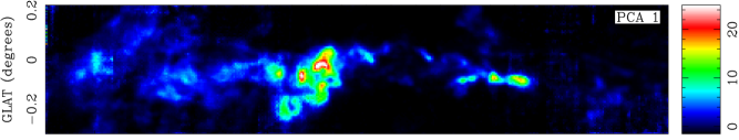
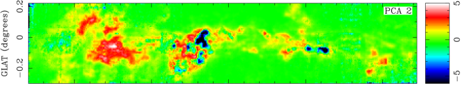
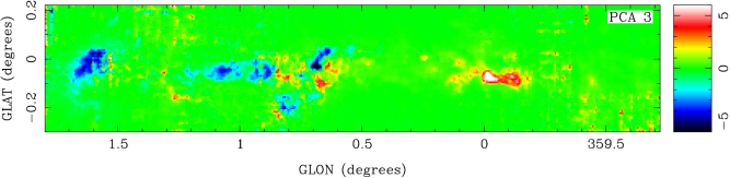
Figure 5: The first three principal component images derived from the ten strongest lines (CS, CH₃OH (at 48.37 GHz), HC₃N, SiO, HNCO, HOCO⁺, NH₂CHO, OCS, C³⁴S and ¹³CS), which describe 68.3, 11.5 and 7.3 percent of the variance respectively. The first principal component describes the common features of the ten lines, and the second principal component describes the most significant differences between the lines. The further principal components describe successively smaller differences.

Figure 6: The component vectors quantifying how the integrated line images are composed of the sum of different scalar amounts of the of the principal component images (Fig. 5).

3.4 Line intensities and line ratios

The previous subsection (3.3) indicates that there are differences in the ratio of lines for different areas within the CMZ. We can quantify this by integrating the line emission over different apertures. The apertures chosen are listed in Table 3 and plotted in Fig. 7. The six regions are the entire region of the CMZ that we have mapped, the four main emission features namely Sgr A, Sgr B2, Sgr C and G1.3, and a smaller region around the core of Sgr B2. They are effectively the same as those used in Jones et al. (2012) for similar analysis of the CMZ in 3-mm lines, with very minor changes due to the data at 7-mm being on different (coarser) pixels to the previous 3-mm data.

Table 3: Apertures selected for analysis. The areas are rectangles in Galactic coordinates, centred on $l$ and $b$. The projected area on the sky assumes a distance of 8.0 kpc.

Region	$l$	$b$	Width	Height	Area	Area
	deg	deg	arcmin	arcmin	arcmin2	pc2
CMZ	0.545	-0.035	151.2	30.0	4 536	24 600
Sgr A	0.042	-0.055	30.8	13.2	406	2 200
Sgr B2	0.735	-0.045	29.2	18.4	537	2 910
Sgr C	-0.462	-0.145	20.0	16.8	336	1 820
G1.3	1.325	0.015	24.0	20.8	499	2 700
Sgr B2	0.675	-0.025	6.0	6.4	38.4	208
Core

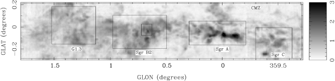
Figure 7: The six areas selected for analysis: around Sgr A, Sgr B2, Sgr C, G1.3, a smaller area at the Sgr B2 core, and the larger CMZ area, plotted on the peak CS emission.

Table 4 presents the integrated line fluxes for these apertures, as $\int\!\!\!\int T_{B}\,\mathrm{d}v\,\mathrm{d}A$ in K km s^-1 pc². The brightness temperature $T_{B}$ is the extended beam temperature, corrected for the extended aperture efficiency of $\sim$ 0.65 (Urquhart et al., 2010), as discussed below.

The line emission is integrated over velocity, with the accuracy limited by low level baseline ripples in the spectra, as discussed in subsection 3.1. To reduce this problem, we integrated over a velocity range which covers the expected emission while excluding too much extra data in the cubes. Hence this velocity range varies with the area (due to differential velocity across the CMZ, and different velocity widths in the different areas) and the line. Uncertainties are quoted, based on observed integrated intensities fluctuations, caused by these baseline offsets, over parts of the data cubes without lines. However, we do note that the baseline ripples vary between the different lines, as does the noise in the cubes (Table 2), so that these uncertainty estimates are only indicative.

These line luminosities can be compared to those of 3-mm lines over the same areas in Jones et al. (2012), and are quoted in the form of $\int\!\!\!\int T_{B}\,\mathrm{d}v\,\mathrm{d}A$ for ease of comparison with other galaxies.

We do not include all the lines in this table, but exclude the weakest lines which are generally below the 3 $\sigma$ level of significance in the areas given the baseline problems (H¹³CCCN, HCC¹³CN, HC₅N, SiO masers, RRLs).

Table 5 presents the integrated line fluxes over the six apertures, normalised by the value for the CS line. The Sgr B2 area generally has an enhanced line flux ratio to CS, as compared to the other areas, and the sub-area Sgr B2 Core has even more enhanced line ratios. While we expect Sgr B2 to be chemically rich, the high ratios relative to CS are likely to be in part due to the high optical depth of CS in this area. This can be checked with the isotopologues ¹³CS and C³⁴S. These do indeed show higher C³⁴S/CS ratio in Table 5 at Sgr B2, and particularly at the Core, which indicates high optical depth in CS. Expressed in the more commonly used form of the ratio CS/C³⁴S (i.e. the inverse to that tabulated) this is lower ratio CS/C³⁴S in Sgr B2 (8.8) and the Sgr B2 Core (7.5) compared to the other regions. The situation in the weaker ¹³CS line is less clear, with lower CS/¹³CS at the Sgr B2 Core, of 14 compared to the expected optically thin value of 24 for the Galactic Centre from Langer & Penzias (1990), but overall ratio 20 in the larger Sgr B2 region (and an anomalously high ratio 63 for Sgr C, which may indicate baselevel problems).

Table 4: Integrated line fluxes as $\int\!\!\!\int T_{B}\,\mathrm{d}v\,\mathrm{d}A$, integrated over velocity, and the areas given in Table 3. The integrated fluxes are in units 10³ K km s^-1 pc², The 1 $\sigma$ uncertainties are given, and the upper limits are at the 3 $\sigma$ level.

Line	CMZ	Sgr A	Sgr B2	Sgr C	G1.3	Sgr B2 Core
CS	1590 $\pm$ 80	218 $\pm$ 11	297 $\pm$ 15	157 $\pm$ 8	246 $\pm$ 12	33.2 $\pm$ 1.7
CH3OH	650 $\pm$ 30	66 $\pm$ 4	182 $\pm$ 9	48 $\pm$ 2.5	130 $\pm$ 7	29.4 $\pm$ 1.5
HC3N	287 $\pm$ 15	33.2 $\pm$ 2.2	82 $\pm$ 5	16.6 $\pm$ 1.0	57 $\pm$ 3	15.1 $\pm$ 0.8
SiO	283 $\pm$ 15	24.8 $\pm$ 1.9	71 $\pm$ 4	14.4 $\pm$ 1.0	72 $\pm$ 4	8.5 $\pm$ 0.5
HNCO	312 $\pm$ 16	23.2 $\pm$ 1.8	80 $\pm$ 5	14.6 $\pm$ 1.0	66 $\pm$ 3	12.9 $\pm$ 0.7
HOCO+	30 $\pm$ 5	$<$ 4	8.0 $\pm$ 2.5	$<$ 1.9	5.5 $\pm$ 0.9	1.69 $\pm$ 0.28
NH2CHO	20 $\pm$ 5	$<$ 4	7.9 $\pm$ 2.5	$<$ 1.9	4.1 $\pm$ 0.9	1.36 $\pm$ 0.28
OCS	60 $\pm$ 6	$<$ 4	25.2 $\pm$ 2.7	$<$ 1.9	16.6 $\pm$ 1.2	3.6 $\pm$ 0.3
HCS+	27 $\pm$ 5	5.2 $\pm$ 1.4	$<$ 7	$<$ 1.9	3.9 $\pm$ 0.9	1.11 $\pm$ 0.28
CCS	34 $\pm$ 6	$<$ 4	13.5 $\pm$ 2.5	$<$ 1.9	8.4 $\pm$ 0.9	2.00 $\pm$ 0.29
C34S	114 $\pm$ 8	9.7 $\pm$ 1.5	33.5 $\pm$ 2.9	10.5 $\pm$ 0.8	19.8 $\pm$ 1.3	4.4 $\pm$ 0.4
13CS	56 $\pm$ 6	11.6 $\pm$ 1.5	14.8 $\pm$ 2.5	2.5 $\pm$ 0.6	9.3 $\pm$ 1.0	2.4 $\pm$ 0.3
29SiO	22 $\pm$ 5	$<$ 4	$<$ 7	2.0 $\pm$ 0.6	3.0 $\pm$ 0.9	$<$ 0.8
CH3OH maser	53 $\pm$ 6	9.6 $\pm$ 1,5	12.0 $\pm$ 2.5	4.0 $\pm$ 0.6	10.1 $\pm$ 1.0	4.0 $\pm$ 0.3

Table 5: Integrated line fluxes, integrated over velocity and the areas given in Table 3, normalised to CS. The 1 $\sigma$ uncertainties are given, and the upper limits are at the 3 $\sigma$ level.

Line	CMZ	Sgr A	Sgr B2	Sgr C	G1.3	Sgr B2 Core
CS	1.00 def.	1.00 def.	1.00 def.	1.00 def.	1.00 def.	1.00 def.
CH3OH	0.41 $\pm$ 0.03	0.301 $\pm$ 0.022	0.61 $\pm$ 0.05	0.306 $\pm$ 0.022	0.53 $\pm$ 0.04	0.89 $\pm$ 0.06
HC3N	0.181 $\pm$ 0.013	0.152 $\pm$ 0.013	0.278 $\pm$ 0.021	0.106 $\pm$ 0.008	0.230 $\pm$ 0.017	0.46 $\pm$ 0.03
SiO	0.178 $\pm$ 0.013	0.113 $\pm$ 0.010	0.238 $\pm$ 0.019	0.092 $\pm$ 0.008	0.291 $\pm$ 0.021	0.255 $\pm$ 0.020
HNCO	0.197 $\pm$ 0.014	0.106 $\pm$ 0.010	0.270 $\pm$ 0.021	0.093 $\pm$ 0.008	0.270 $\pm$ 0.019	0.39 $\pm$ 0.03
HOCO+	0.019 $\pm$ 0.004	$<$ 0.019	0.027 $\pm$ 0.008	$<$ 0.012	0.022 $\pm$ 0.004	0.051 $\pm$ 0.009
NH2CHO	0.013 $\pm$ 0.003	$<$ 0.019	0.027 $\pm$ 0.008	$<$ 0.012	0.017 $\pm$ 0.004	0.041 $\pm$ 0.009
OCS	0.038 $\pm$ 0.004	$<$ 0.019	0.085 $\pm$ 0.010	$<$ 0.012	0.067 $\pm$ 0.006	0.109 $\pm$ 0.011
HCS+	0.017 $\pm$ 0.004	0.024 $\pm$ 0.007	$<$ 0.024	$<$ 0.012	0.016 $\pm$ 0.004	0.033 $\pm$ 0.008
CCS	0.021 $\pm$ 0.004	$<$ 0.019	0.046 $\pm$ 0.009	$<$ 0.012	0.034 $\pm$ 0.004	0.060 $\pm$ 0.009
C34S	0.072 $\pm$ 0.006	0.044 $\pm$ 0.007	0.113 $\pm$ 0.011	0.067 $\pm$ 0.006	0.080 $\pm$ 0.007	0.133 $\pm$ 0.012
13CS	0.035 $\pm$ 0.004	0.053 $\pm$ 0.007	0.050 $\pm$ 0.009	0.016 $\pm$ 0.004	0.038 $\pm$ 0.004	0.073 $\pm$ 0.010
29SiO	0.014 $\pm$ 0.003	$<$ 0.019	$<$ 0.024	0.013 $\pm$ 0.004	0.012 $\pm$ 0.003	$<$ 0.024
CH3OH maser	0.033 $\pm$ 0.004	0.044 $\pm$ 0.007	0.041 $\pm$ 0.009	0.025 $\pm$ 0.004	0.041 $\pm$ 0.004	0.121 $\pm$ 0.012

3.5 Ratio of 7-mm and 3-mm lines

The observed integrated line intensity $\int T\mathrm{d}v$ of a spectral line can be related to the column density $N_{u}$ of molecules in the upper level of the transition, for optically thin lines using standard assumptions of LTE radiative transfer (Wilson, Rohlfs & Hüttemeister, Wilson et al.2009), by $N_{u}=(8\pi\nu^{2}k/hc^{3}A_{ul})\int T_{B}\mathrm{d}v$, where $A_{ul}$ is the Einstein coefficient. The total column density $N$ of the molecule is given by $N=(N_{u}/g_{u})Q_{T}\exp(E_{u}/kT_{ex})$ where $Q_{T}(T_{ex})$ is the partition function, $T_{ex}$ is the excitation temperature, $E_{u}$ is the energy of the upper level and $g_{u}$ is the statistical weight of the upper level.

The excitation temperature $T_{ex}$ describes the relative populations in different levels, and is typically not the same as the gas kinetic temperature $T_{kin}$, as at low densities the excitation depends on the radiation as well as collisions (, Wilson et al.2009).

As we have 3-mm line observations of the CMZ from Jones et al. (2012) to match the 7-mm observations here, we can consider the ratio of integrated line intensities $\int T\mathrm{d}v$, which is related (subject to assumptions, and caveats below) to the excitation temperature $T_{ex}$.

We consider five molecules, that is HNCO, HOCO⁺, HC₃N, SiO and ¹³CS, common to both our 7-mm and 3-mm CMZ spectral imaging. The 3-mm data were smoothed to the resolution of the 7-mm data, using the beamsizes (62 to 68 arcsec) interpolated from the Mopra 7-mm measurements of Urquhart et al. (2010). The 3-mm and 7-mm data expressed as $T_{A}^{*}$ were converted to brightness temperatures $T_{B}$ appropriate for extended emission which fills both the main beams and inner sidelobes, by dividing by the extended beam efficiencies at 3-mm (0.62 to 0.65) and 7-mm (0.66 to 0.69) interpolated from Ladd et al. (2005) and Urquhart et al. (2010) respectively.

The ratio image of $\int T_{B}\mathrm{d}v$ for the 3-mm and 7-mm lines was taken by summing 3-dimensional pixels (voxels) over velocity in both cubes, over the region where both lines were above the respective 3-$\sigma$ level, and then dividing the integrated emission images. This reduces the effect of including data without significant emission which adds artifacts due to low-level baseline offsets (particularly in the 3-mm data which is more weather affected), but should not bias the ratio due to missing flux, as we consider the ratio of emission from the same voxels. It is effectively a weighted mean of the ratio, considered on a voxel basis, with the weighting set to zero below the 3-$\sigma$ level.

The ratio images are presented in Fig. 8 as the natural logarithm of the ratio of 3-mm to 7-mm $\int T_{B}\mathrm{d}v$, $\ln(\int T_{B,3mm}\mathrm{d}v/\int T_{B,7mm}\mathrm{d}v)$. The HNCO, HOCO⁺ and HC₃N images show variations in the ratio across the CMZ, in the sense that the 3-mm to 7-mm ratio is higher around Sgr B2 and Sgr A, and is less around longitudes 1.0 deg. to 1.8 deg. There are some signs of similar variation in the ratio in the SiO image, but less clearly.

The ratios are plotted in Fig. 9 averaged over latitude, to show the longitude variations more clearly. The plots for HOCO⁺ and ¹³CS are noisy for longitude ranges with little data, but the HOCO⁺ does show the difference in ratio between Sgr B2 and higher longitudes. The plots for HNCO, HC₃N and SiO do show ratio variations.

At the centre of Sgr B2 in Fig. 8 there is a small region of higher 3-mm to 7-mm ratio in HC₃N, SiO and ¹³CS, associated with the free-free radio peak of Sgr B2. We attribute this to the radiative transfer effect of line emission being absorbed in front of the strong continuum. This occurs to a greater extent in the 7-mm band compared to the 3-mm band, as discussed in Jones et al. (2012), leading to the enhanced 3-mm to 7-mm ratio.

The line ratio differences can largely be interpreted as excitation temperature differences, as discussed above, with the caveat that other effects may be occuring, such as the continuum absorption and signifcant optical depth (subsection 3.3). The line frequencies ($\nu$), Einstein coefficients ($A_{ul}$), statistical weights ($g_{u}$) and upper energy levels ($E_{u}$) were obtained from the splatalogue online compilation (http://www.splatalogue.net/).

The statistics of the line ratios $\ln(\int T_{B,3mm}\mathrm{d}v/\int T_{B,7mm}\mathrm{d}v)$ (mean and standard deviation) are listed in Table 6, for the areas in Table 3and Fig. 7. The corresponding excitation temperatures $T_{ex}$ assuming optically thin LTE conditions are listed in Table 7.

Note that these calculated excitation temperatures $T_{ex}$ are much lower than the kinetic temperature $T_{kin}\sim$  30 K. In practice, for the likely physical conditions in the CMZ, the energy levels of these molecules are unlikely to be in LTE (see below, section 4). Hence the values of $T_{ex}$ calculated here are a useful way to describe the relative populations of the levels that give rise to the 7-mm and 3-mm lines, but should not be over-interpreted as applying to other levels.

We note the line ratios are smaller beyond Sgr B2, and thus outside the $\rm 10^{7}\,M_{\odot}$ rotating dust ring, that extends from Sgr B2 to Sgr A, citepmo+11. This is particularly noticeable with the G1.3 dust core, where the higher excitation 3-mm lines are relatively weaker.

Table 6: Mean and standard deviation of the ratio of 3-mm to 7-mm lines, expressed as $\ln$(ratio), ie $\ln(T_{3mm}/T_{7mm})$ in the selected areas.

Molecule	CMZ	Sgr A	Sgr B2	Sgr C	G1.3	Sgr B2 Core
HNCO	$0.07\pm 0.32$	$0.37\pm 0.24$	$0.43\pm 0.21$	$0.16\pm 0.25$	$-0.14\pm 0.13$	$0.58\pm 0.11$
HOCO+	$-0.04\pm 0.33$	$0.28\pm 0.29$	$0.07\pm 0.29$	$-0.12\pm 0.15$ #	$-0.13\pm 0.14$ #	$0.39\pm 0.23$
HC3N	$-0.71\pm 0.32$	$-0.48\pm 0.24$	$-0.63\pm 0.28$	$-0.58\pm 0.25$	$-0.83\pm 0.28$	$-0.45\pm 0.23$
SiO	$-0.30\pm 0.18$	$-0.22\pm 0.14$	$-0.25\pm 0.15$	$-0.21\pm 0.21$	$-0.34\pm 0.14$	$-0.25\pm 0.13$
13CS	$-0.36\pm 0.25$	$-0.30\pm 0.16$	$-0.37\pm 0.17$	$-0.23\pm 0.18$	$-0.35\pm 0.16$ #	$-0.31\pm 0.22$

# = small number of pixels ($<100$) with good data (clipped at 3 $\sigma$.)

Table 7: The excitation temperatures $T_{ex}$ in K, assuming optically-thin LTE conditions, derived from the ratio of 3-mm to 7-mm lines. Note, however, that radex modelling in section 4 shows that assuming optically-thin LTE is too simplistic.

Molecule	CMZ	Sgr A	Sgr B2	Sgr C	G1.3	Sgr B2 Core
HNCO	$5.6^{+1.8}_{-1.1}$	$7.3^{+2.3}_{-1.4}$	$7.7^{+2.2}_{-1.4}$	$6.0^{+1.6}_{-1.0}$	$4.8^{+0.5}_{-0.4}$	$9.2^{+1.5}_{-1.1}$
HOCO+	$5.0^{+1.5}_{-1.0}$	$6.5^{+2.3}_{-1.4}$	$5.5^{+1.5}_{-1.0}$	$4.8^{0.5+}_{-0.4}$ #	$4.7^{+0.5}_{-0.4}$ #	$7.2^{+2.2}_{-1.4}$
HC3N	$8.9^{+1.3}_{-1.0}$	$9.4^{+1.4}_{-1.1}$	$8.7^{+1.4}_{-1.1}$	$8.9^{+1.3}_{-1.0}$	$7.9^{+1.1}_{-0.9}$	$9.5^{+1.4}_{-1.1}$
SiO	$2.5^{+0.3}_{-0.2}$	$2.6^{+0.3}_{-0.2}$	$2.6^{+0.3}_{-0.2}$	$2.6^{+0.4}_{-0.3}$	$2.4^{+0.2}_{-0.2}$	$2.6^{+0.2}_{-0.2}$
13CS	$2.2^{+0.4}_{-0.3}$	$2.2^{+0.2}_{-0.2}$	$2.2^{+0.2}_{-0.2}$	$2.3^{+0.3}_{-0.2}$	$2.2^{+0.4}_{-0.3}$ #	$2.2^{+0.3}_{-0.3}$

# = small number of pixels ($<100$) with good data (clipped at 3 $\sigma$.)

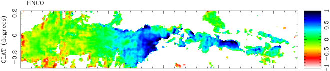
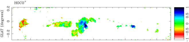
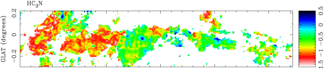
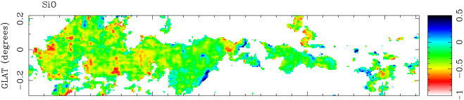
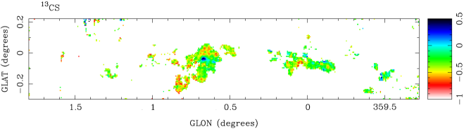
Figure 8: The distribution of the ratio of integrated line brightness of 3-mm to 7-mm lines of HNCO, HOCO⁺, HC₃N, SiO and ¹³CS expressed as $\ln(\int T_{B,3mm}\mathrm{d}v/\int T_{B,7mm}\mathrm{d}v)$.

Figure 9: The ratio of integrated line brightness of 3-mm to 7-mm lines of HNCO, HOCO⁺, HC₃N, SiO and ¹³CS expressed as $\ln(\int T_{B,3mm}\mathrm{d}v/\int T_{B,7mm}\mathrm{d}v)$, averaged over latitude, to show the variation with longitude. Note the variation in line ratio across the CMZ, most clearly shown in HNCO, HC₃N and SiO.

4 Discussion

The kinetic temperature $T_{kin}$ and hydrogen density $n$ in the CMZ have been fitted by Nagai et al. (2007) using CO lines (¹²CO 1–0, ¹²CO 3–2, ¹³CO 1–0) with a Large Velocity Gradient (LVG) model, giving typical values $T_{kin}=30$ K and $n=3\times 10^{3}$ cm^-3.

For such physical conditions $T_{kin}$ and $n$ we can confirm with the non-LTE model RADEX of van der Tak et al. (2007), that the 7-mm and 3-mm lines studied in section 3.5 give a low effective excitation temperature $T_{ex}$. The hydrogen density $n$ is much lower than the critical density $n_{crit}$ at which the collisions would thermalise the molecular levels to $T_{kin}$. We used the online version of RADEX, to explore the parameter space that would reproduce the 7-mm line fluxes and the 3-mm to 7-mm line ratios. We do note that this still assumes an isothermal homogeneous medium.

The input parameters to RADEX are excitation conditions, $T_{kin}$, $n$ and background temperature $T_{bg}$, and radiative transfer parameters, $N$ and line width $\Delta\,v$. If we fix $T_{kin}=30$ K, $\Delta\,v=10$ km s^-1 which is typical of these lines in the CMZ, and $T_{bg}=2.73$ K for the microwave background temperature, then we have two free parameters $n$ and $N$. Varying $n$ changes the relative populations of the molecular levels, and hence the ratio of 3-mm to 7-mm transitions. Varying $N$ changes the line brightness temperature $T_{R}$. With two free parameters, we can fit the two observable parameters, but only if the combination of observable parameters is in the range of the model, so this is not a trivial process. In practice, varying one of $n$ and $N$ changes both the ratio and $T_{R}$ due to non-linearities, such as optical depth.

The results of such modelling is given in Table 8 for four molecules. HOCO⁺ is not one of the molecules with data files available for RADEX. We varied $n$ and $N$ to obtain typical values of $\ln(T_{B,3mm}/T_{B,7mm})$ and $T_{R}$ (for the 7-mm line) given in the data in subsection 3.5. For each molecule, we present four fits, giving a typical $T_{R}$ with mean ratio, higher and lower ratios by 0.3 in the $\ln$(ratio) or factor 1.35, and a fit for mean ratio and higher $T_{R}$.

The derived values of $n$ are a few times 10⁴ cm^-3, which is somewhat larger than the typical value $n=3\times 10^{3}$ cm^-3 obtained by Nagai et al. (2007) for CO, but these molecules with higher $n_{crit}$ preferentially trace higher demsities.

We have shown here that the observed ratio of the 3-mm to 7-mm lines, and the line brightness temperatures, can be fitted with plausible values of $n$ and $N$. With only two lines, we can only constrain two parameters at a time, with other RADEX input parameters fixed. In practice, it is quite likely that the kinetic temperature $T_{kin}$ and background temperature $T_{bg}$ vary across the CMZ as well, so the actual variation in physical conditions is more complcated.

The higher 3-mm to 7-mm line ratios around Sgr B2 and Sgr A, compared to longitudes around G1.3, can be partly explained by higher density $n$, which means that the sub-thermal excitation gets closer to thermalisation with kinetic temperature $T_{kin}$. As noted above, however, from the data and analysis here we cannot rule out changes in $T_{bg}$ and $T_{kin}$ too.

Table 8: Results of RADEX non-LTE models to reproduce typical 3-mm to 7-mm line ratios, and 7-mm line brightness observed in the CMZ. These are labelled m for mean or mid-range, l for low and h for high. We assume fixed $T_{kin}=30$ K, $\Delta\,v=10$ km s^-1 and $T_{bg}=2.7$ K.

Molecule	$n$	$N$	$\ln(T_{3mm}/T_{7mm})$	$T_{R}$
	104 cm-3	1014 cm-2		K
HNCO	0.65	1.7	$-0.24$  l	1.0  m
HNCO	1.1	1.7	$0.08$  m	1.0  m
HNCO	1.7	1.8	$0.37$  h	1.0  m
HNCO	1.2	4.5	$0.08$  m	2.5  h
HC3N	1.8	0.50	$-1.02$  l	1.0  m
HC3N	2.7	0.50	$-0.70$  m	1.0  m
HC3N	3.7	0.50	$-0.41$  h	1.0  m
HC3N	2.5	1.3	$-0.72$  m	2.4  h
SiO	1.5	0.34	$-0.61$  l	0.49  m
SiO	4.2	0.20	$-0.30$  m	0.52  m
SiO	8.0	0.17	$-0.00$  h	0.51  m
SiO	4.5	0.50	$-0.31$  m	1.2  h
13CS	0.50	0.30	$-0.66$  l	0.17  m
13CS	1.5	0.15	$-0.36$  m	0.17  m
13CS	3.0	0.13	$-0.06$  h	0.17  m
13CS	1.5	0.37	$-0.38$  m	0.40  h

5 Summary

We have mapped a $2.5^{\circ}\times 0.5^{\circ}$ region of the Central Molecular Zone (CMZ) of the Galaxy using the Mopra radio telescope in 21 molecular and 3 hydrogen lines emitting from 42–50 GHz. The maps have spatial resolution $\sim 65$ arcsec and spectral resolution $\rm\sim 1.8\,km\,s^{-1}$. For five species the emission is particularly strong and widespread; CS, CH₃OH, HC₃N, SiO and HNCO. For the other molecules emission is generally confined to the bright dust cores around Sgr A, Sgr B2 and G1.3. These data add to, and complement, previous studies we have undertaken in the 85–93 and 20–28 GHz portions of the mm-spectrum. As also seen in these other bands the molecular emission at 42–50 GHz is both widespread, but asymmetric, about the Galactic Centre, and turbulent.

Principal component analysis (PCA) of the ten brightest emission lines quantifies the similarities and differences, with the first component, representing an averaged integrated map of all the molecular lines, contributing 68% of the variance shown in the data. The second component contributes 12% to the variance and highlights some differences in the dust cores, attributable to the brightest lines being optically thick in them. The third component contributes 7% to the variance and highlights some chemical differences, with HOCO⁺, HNCO and OCS being particularly prominent in G1.6 and Sgr B2.

Line fluxes and luminosities are presented for the brightest dust cores, as well as for the entire CMZ, to aid in comparison with observations of nuclei of external galaxies where such components would be unresolved.

Combining the data set with the higher-excitation lines we have mapped in the 3 mm band for five of the species (HNCO, HOCO⁺, HC₃N, SiO and ${}^{13}CS$) which indicates variations in the line ratios across the CMZ, with larger 3-mm to 7-mm line ratios observed outside the $\rm 10^{7}\,M_{\odot}$ rotating dust ring, in particular for the molecular cloud complex G1.3. This implies cooler temperatures for the molecular gas here than in the dust ring.

All these species are sub-thermally excited across the CMZ, with excitation temperatures considerably less than the kinetic temperature. Modelling of the emission using RADEX suggests gas densities for these molecules are, in general, a few $\rm\times 10^{4}\,cm^{-3}$, a factor of a few higher than corresponding densities derived from CO line measurements.

The full data set, comprising the data cubes for the 21 molecular plus 3 hydrogen lines, is publicly available through the Australia Telescope National Facility archives (http://atoa.atnf.csiro.au/CMZ). A final data set in this series, consisting of data on the isotopologues of the CO J=1–0 lines over a $5^{\circ}\times 1.5^{\circ}$ of the CMZ, is currently being prepared for publication.

References

- Amo-Baladrón, Martín-Pintado, & Martín (2011) Amo-Baladrón M. A., Martín-Pintado J., Martín S., 2011, A&A, 526, A54
- (2) Ferrière K., Gillard W., Jean P., 2007, A&A, 467, 611
- Jones et al. (2008a) Jones P. A., et al., 2008a, MNRAS, 386, 117
- Jones et al. (2008b) Jones P. A., Burton M. G., Lowe V., 2008b, in Kwok S., Sandford S, eds, Organic Matter in Space, Proc. IAU Symp., 251, Cambridge Univ. Press, Cambridge, p. 257
- Jones et al. (2011) Jones P. A., Burton M. G., Tothill N.F.H., Cunningham M. R., 2011, MNRAS, 411, 2293
- Jones et al. (2012) Jones P. A., et al., 2012, MNRAS, 419, 2961
- Ladd et al. (2005) Ladd N., Purcell C., Wong T., Robertson S., 2005, PASA, 22, 62
- Langer & Penzias (1990) Langer W. D., Penzias A. A., 1990, ApJ, 357, 477
- Lo et al. (2009) Lo N., et al., 2009, MNRAS, 395, 1021
- Longmore et al. (2012) Longmore S. N., et al., 2013, MNRAS, 429, 987
- Lovas & Dragoset (2004) Lovas F.J., Dragoset R.A., 2004, J. Phys. Chem. Ref. Data 33, 177
- Martín et al. (2008) Martín S., Requena-Torres M. A., Martín-Pintado J., Mauersberger R., 2008, ApJ, 678, 245
- Molinari et al. (2011) Molinari S., et al., 2011, ApJ, 735, L33
- Morris & Serabyn (1996) Morris M., Serabyn E., 1996, ARA&A, 34, 645
- Nagai et al. (2007) Nagai M., Tanaka K., Kamegai K., Oka T., 2007, PASJ, 59, 25
- Purcell et al. (2012) Purcell C. R., et al., 2012, MNRAS, 426, 1972
- Reid et al. (2009) Reid M. J., Menten K. M., Zheng X. W., Brunthaler A., Xu Y., 2009, ApJ, 705, 1548
- Urquhart et al. (2010) Urquhart, J. S., et al., 2010, PASA, 27, 321
- van der Tak et al. (2007) van der Tak F. F. S., Black J. H., Schöier F. L., Jansen D. J., van Dishoeck E. F., 2007, A&A, 468, 627
- Walsh et al. (2008) Walsh A. J., Lo N., Burton M. G., White G. L., Purcell C. R., Longmore S. N., Phillips C. J., Brooks K. J., 2008, PASA, 25, 105
- Walsh et al. (2011) Walsh A. J., et al., 2011, MNRAS, 416, 1764
- (22) Wilson T. L., Rohlfs K., Hüttemeister S., 2009, Tools of Radio Astronomy, Springer, Berlin