Mixed Mimetic Spectral Element method applied to Darcy’s problem

Abstract

We present a discretization for Darcy’s problem using the recently developed Mimetic Spectral Element Method kreeft2011mimetic . The gist lies in the exact discrete representation of integral relations. In this paper, an anisotropic flow through a porous medium is considered and a discretization of a full permeability tensor is presented. The performance of the method is evaluated on standard test problems, converging at the same rate as the best possible approximation.

1 DARCY FLOW

Anisotropic heterogeneous diffusion problems are ubiquitous across different scientific fields, such as, hydrogeology, oil reservoir simulation, plasma physics, biology, etc herbin2008benchmark . Darcy’s equation describes a steady pressure-driven flow through a porous medium where fluxes and pressure are linearly related,

$$\text{div}\ \frac{\mathbb{K}}{\mu}\ \text{grad}\ p=\phi\overset{\mu=1}{\longrightarrow}\left\{\begin{array}[]{llr}\vec{u}-\text{grad}\ p=0&\text{in }\Omega&(1\mathrm{a})\\ \text{div}\ \vec{q}=\phi&\text{in }\Omega&(1\mathrm{b})\\ \vec{q}=\mathbb{K}\vec{u}&\text{in }\Omega&(1\mathrm{c})\\ \vec{q}=\vec{q_{0}}&\text{in }\partial\Omega&(1\mathrm{d})\\ \end{array}\right.$$

where $\vec{u}$ is the fluid velocity, $p$ the pressure, $\vec{q}$ the mass flux and $\phi$ the prescribed source term. Without loss of generality let the viscosity, $\mu=1$, and consider a permeability symmetric, positive definite tensor denoted by $\mathbb{K}$.

In a three-dimensional setting are: four types of submanifolds (points, lines, surfaces and volumes); and two orientations (outer and inner, as an example see Figure 1). Tessellation divides the physical domain in a set of these geometric objects to which we associate discrete variables, i.e. integral quantities. Thus, associated with every physical variable is a correspondent geometric object, this symbiotic relation between physics and geometry is the core of mimetic methods. Many scholars are aware of this relationship bossavit2005discretization ; burke1985applied ; frankel ; tonti1975formal .

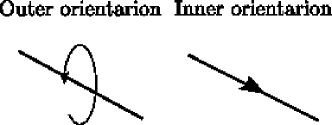
Figure 1: Consider a line where we can have two types of orientation: Outer - around the line; Inner - along the line.

Starting from the mass balance equation, $(1\mathrm{b})$,

$$\int_{V}\text{div}\ \vec{q}\ \mathrm{d}V=\int_{\partial V}\vec{q}\cdot\vec{n}\ \mathrm{d}S=\int_{V}\phi\ \mathrm{d}V,$$ (2)

it is clear that the divergence in a volume is equal to the sum of the surface integral quantities, i.e. oriented fluxes. Thus, we will associate mass fluxes, $\vec{q}$, with quantities that go through surfaces. This equation therefore tells us that the right hand side term $\phi$ is associated to outer-oriented volumes.

Similarly, using Newton-Leibniz relation for equation $(1\mathrm{a})$,

$$\int_{C}\text{grad}\ p\ \mathrm{d}C=\int_{\partial C}p=p\left(B\right)-p\left(A\right)=\int_{C}\vec{u}\ \mathrm{d}C,$$ (3)

the fluid velocity, $\vec{u}$, is represented along lines and $p$ is represented by the values in points. From (3) we deduces that $u$ and $p$ are inner-oriented variables.

The constitutive/material relation relation $(1\mathrm{c})$ is given by,

$$\vec{q}=\mathbb{K}\vec{u},$$ (4)

which defines how quantities associated to inner-oriented lines relate to quantities associated to outer-oriented surfaces. Whereas equation $(2)$ and $(3)$ can be exactly satisfied on a finite grid the constitutive equation $(4)$ needs to be approximated.

The importance of respecting the geometric nature in physics is discussed in gerritsmaICOSAHOM . Figure 2 summarizes the geometric character of the Darcy’s problem.

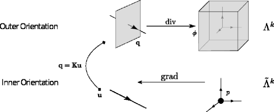
Figure 2: Darcy’s flow problem geometric characterization. Fluxes, $\vec{q}$, are associated with outer oriented surfaces; $\phi$, is associated with outer oriented volumes; velocity, $\vec{u}$, is associated with inner oriented lines; pressure, $p$, is associated with inner oriented points

We will denote the space of variables associated to outer-oriented $k$-dimensional objects by $\Lambda^{k}\left(\mathcal{M}\right)$ and the space of variables associated to inner-oriented $k$-dimensional objects by $\tilde{\Lambda}^{k}\left(\mathcal{M}\right)$ as indicated in Figure 2.

In this paper we will make use of the spectral element method described in gerritsmaICOSAHOM ; kreeft2011mimetic , application of these ideas to Stokes’ flow see KreeftICOSAHOM ; kreeft2012priori ; kreeft::stokes ; Poisson equation for volume forms palhaLaplaceDualGrid ; advection equation palhaAdvection ; derivation of a momentum conservation scheme ToshniwalICOSAHOM . Extension to compatible isogeometric methods see HiemstraICOSAHOM ; hiemstra2012high . For applications of these ideas in a finite difference setting see Brezzi et al. BrezziBuffaLipnikov2009 . In the context of finite element methods Arnold, Falk and Winther arnold2010finite proposed a Finite Element Exterior Calculus. In a more geometric spirit Desbrun et al. desbrun2005discrete and Hirani Hirani_phd_2003 developed the discrete exterior calculus (DEC). An application of the latter to Darcy flow can be found in hirani2008numerical .

2 DISCRETIZATION OF EQUATIONS

In this section we will describe the discretization by defining the weak formulation. The approached followed here is similar to hyman1997numerical ; jerome2012analysis .

For vectors associated with outer-oriented surfaces, $\Lambda^{2}\left(\mathcal{M}\right)$, we define the weighted inner product

$$\left(\mathbf{a},\mathbf{b}\right)_{\mathcal{M},\mathbb{K}}=\int_{\mathcal{M}}\mathbf{a}\mathbb{K}^{-1}\mathbf{b}\ \mathrm{d}V.$$ (5)

Furthermore, we define bilinear maps $((\cdot,\cdot))_{\mathcal{M}}\,:\,\Lambda^{1}\left(\mathcal{M}\right)\times\tilde{\Lambda}^{n-1}\left(\mathcal{M}\right)\rightarrow\mathbb{R}$

$$((\mathbf{u},{\mathbf{\tilde{v}}}))_{\mathcal{M}}:=\int_{\mathcal{M}}\mathbf{u}\cdot\mathbf{\tilde{v}}\ \mathrm{d}V.$$ (6)

and $((\cdot,\cdot))_{\mathcal{M},\mathbb{K}}\,:\,\Lambda^{k}\left(\mathcal{M}\right)\times\tilde{\Lambda}^{n-k}\left(\mathcal{M}\right)\rightarrow\mathbb{R}$ given by

$$(({\mathbf{u}},{\mathbf{\tilde{v}}}))_{\mathcal{M},\mathbb{K}}:=\int_{\mathcal{M}}\mathbf{u}\cdot\mathbb{K}^{-1}\mathbf{\tilde{v}}\ \mathrm{d}V.$$ (7)

For $\mathbf{q}\in\Lambda^{2}\left(\mathcal{M}\right)$ and $p\in\tilde{\Lambda}^{0}\left(\mathcal{M}\right)$ and homogeneous boundary values we have

$$\left(\left(\text{div}\mathbf{q},\ {p}\right)\right)_{\mathcal{M}} =-\left(\left(\mathbf{q},\text{grad}p\right)\right)_{\mathcal{M}}$$ (8)

$$=-\left(\left(\mathbf{q},\mathbb{K}^{-1}\left[\mathbb{K}\ \text{grad}p\right]\right)\right)_{\mathcal{M}}$$

$$=\left(\left(\mathbf{q},\text{grad}_{\mathbb{K}}^{*}\ p\right)\right)_{\mathcal{M},\mathbb{K}}.$$

It is possible to define a new gradient operator,

$$\text{grad}_{\mathbb{K}}^{*}=-\mathbb{K}\ \text{grad}.$$ (9)

Mixed formulation

Starting from (1) and making use of the bilinear maps defined above we have for all vectors $\boldsymbol{\tau}\in\Lambda^{n-1}\left(\mathcal{M}\right)$ associated to outer-oriented surfaces

$$\left(\left(\boldsymbol{\tau},\vec{u}-\text{grad}p\right)\right)_{\mathcal{M}} =0$$ (10)

$$\Longleftrightarrow$$

$$\left(\left(\boldsymbol{\tau},\mathbb{K}\vec{u}-\mathbb{K}\text{grad}p\right)\right)_{\mathcal{M},\mathbb{K}} =0$$

$$\stackrel{{\scriptstyle(\ref{def:grad_star})}}{{\Longleftrightarrow}}$$

$$\left(\left(\boldsymbol{\tau},\mathbb{K}\vec{u}\right)\right)_{\mathcal{M},\mathbb{K}}+\left(\boldsymbol{\tau},\text{grad}^{*}_{\mathbb{K}}p\right)_{\mathcal{M},\mathbb{K}} =0$$

$$\stackrel{{\scriptstyle(1\mathrm{c})\mbox{ and }(\ref{eq::adjointGradientDivergence})}}{{\Longleftrightarrow}}$$

$$\left(\boldsymbol{\tau},\vec{q}\right)_{\mathcal{M},\mathbb{K}}+\left(\left(\text{div}\ \boldsymbol{\tau},\ p\right)\right)_{\mathcal{M}} =0$$

The constitutive equation is included in the last step by converting the bilinear form to a weighted inner product on $\Lambda^{2}\left(\mathcal{M}\right)$ as defined in (5). For $(1\mathrm{b})$ we take the bilinear map for the divergence of a vector $\mathbf{q}$ associated with outer-oriented surfaces and an arbitrary scalar function defined in inner-oriented points, $\gamma\in\tilde{\Lambda}^{0}\left(\mathcal{M}\right)$,

$$\left(\left({\text{div}\mathbf{q}},{\gamma}\right)\right)_{\mathcal{M}} =\left(\left({\phi},{\gamma}\right)\right)_{\mathcal{M}}.$$ (11)

The mixed formulation becomes: Find $\left(\mathbf{q},p\right)\in\left\{\Lambda^{2}\left(\mathcal{M}\right)\times\tilde{\Lambda}^{0}\left(\mathcal{M}\right)\right\}$, given $\phi\in\Lambda^{3}\left(\mathcal{M}\right)$, for all $\left(\boldsymbol{\tau},\gamma\right)\in\left\{\Lambda^{2}\left(\mathcal{M}\right)\times\tilde{\Lambda}^{0}\left(\mathcal{M}\right)\right\}$ such that,

$$\left(\tau,\mathbf{q}\right)_{\mathcal{M},\mathbb{K}}+\left(\left(\text{div}\ \boldsymbol{\tau},\ p\right)\right)_{\mathcal{M}} =0$$ (12)

$$\left(\left({\text{div}\mathbf{q}},{\gamma}\right)\right)_{\mathcal{M}} =\left(\left({\phi},{\gamma}\right)\right)_{\mathcal{M}}\;.$$ (13)

2.1 Basis functions

For the high order representation we use Lagrange, $l_{i}\left(\xi\right)$, and edge functions, $e_{i}\left(\xi\right)$. Lagrange polynomials interpolate nodal values. The edge functions, derived by Gerritsma gerritsma::edge_basis are constructed such that when integrating over a line segment it gives one for the corresponding element and zero for any other line segment,

$$l_{i}\left(\xi_{j}\right)=\delta_{i,j}\qquad\int_{\xi_{j-1}}^{\xi_{j}}e_{i}\left(\xi\right)=\delta_{i,j}.$$ (14)

The relation between the Lagrange and the edge functions is given by,

$$e_{i}\left(\xi\right)=\epsilon_{i}\left(\xi\right)d\xi,\quad\text{with}\quad\epsilon_{i}\left(\xi\right)=-\sum_{k=0}^{i-1}\frac{dl_{k}}{d\xi}.$$ (15)

Note that this definition implies

$$\frac{dl_{i}}{d\xi}=e_{i}(\xi)-e_{i+1}(\xi)\;.$$ (16)

Extension to the multidimensional is obtained by means of tensor products. For more details see kreeft2011mimetic .

2.2 Mimetic discretization in 2D

Expansion of unknowns in $\mathbb{R}^{2}$

Let $\mathbf{q}\in\Lambda^{1}\left(\mathcal{M}\right)$ be expanded as,

$$\mathbf{q}_{h}=\left[\begin{array}[]{c}\sum\limits_{i=0}^{N}\sum\limits_{j=1}^{N}q_{i,j}^{x}l_{i}\left(\xi\right)e_{j}\left(\eta\right)\\ \sum\limits_{i=1}^{N}\sum\limits_{j=0}^{N}q_{i,j}^{y}e_{i}\left(\xi\right)l_{j}\left(\eta\right)\end{array}\right]\;,$$ (19)

and the pressure, $p_{h}\in\tilde{\Lambda}^{0}\left(\mathcal{M}\right)$ as,

$$p_{h}=\sum\limits_{i=1}^{N}\sum\limits_{j=1}^{N}p_{i,j}\epsilon_{i}\left(\xi\right)\epsilon_{j}\left(\eta\right).$$ (20)

Discrete divergence in $\mathbb{R}^{2}$

The divergence of $\mathbf{q}_{h}$ is then given by

$$\text{div}\ \vec{q}_{h} =\sum\limits_{i=1}^{N}\sum\limits_{j=1}^{N}\left(q_{i,j}^{x}-q_{i-1,j}^{x}+q_{i,j}^{y}-q_{i,j-1}^{y}\right)e_{i}\left(\xi\right)e_{j}\left(\eta\right)\;,$$ (21)

where we repeatedly used (16). The scalar $\phi\in\Lambda^{2}\left(\mathcal{M}\right)$ associated with outer-oriented volumes is expanded as

$$\phi_{h} =\sum\limits_{i=1}^{N}\sum\limits_{j=1}^{N}\phi_{i,j}e_{i}\left(\xi\right)e_{j}\left(\eta\right)\;.$$ (22)

Equating (21) and (22) yields

$$\sum\limits_{i=1}^{N}\sum\limits_{j=1}^{N}\phi_{i,j}\bcancel{e_{i}\left(\xi\right)e_{j}\left(\eta\right)} =\sum\limits_{i=1}^{N}\sum\limits_{j=1}^{N}\left(q_{i,j}^{x}-q_{i-1,j}^{x}+q_{i,j}^{y}-q_{i,j-1}^{y}\right)\bcancel{e_{i}\left(\xi\right)e_{j}\left(\eta\right)}$$ (23)

$$\left[\phi\right] =\mathsf{E}^{(2,1)}\left[\vec{q}\right].$$ (24)

We see that the basis functions cancel from this relation. The matrix $\mathsf{E}^{(2,1)}$ relates the fluxes $q_{i,j}^{x}$ and $q_{i,j}^{y}$ to the volume integral $\phi_{i,j}$, as depicted in Figure 3. This fully discrete equation is a restatement of the integral relation (2). The matrix $\mathsf{E}^{(2,1)}$ only contains the values $-1$, $0$ and $1$ and is fully determined by the grid, see kreeft2011mimetic . This is an incidence matrix showing the topological nature of the discrete divergence.

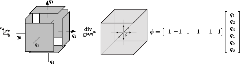
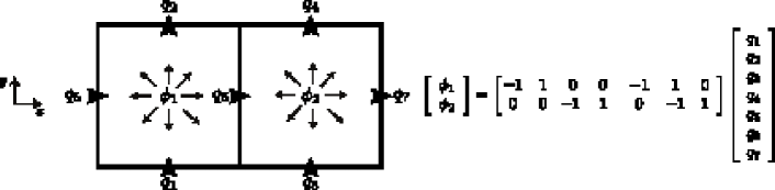
Figure 3: Discrete representation of the action of the divergence in $\mathbb{R}^{3}$ and $\mathbb{R}^{2}$.

If we insert the expansions of our unknowns in (12) and (13) we obtain in $\mathbb{R}^{n}$ the saddle point problem given by,

$$\left[\begin{array}[]{cc}\texttimes M^{(n-1)}_{\mathbb{K}}&\left(\mathsf{E}^{(n,n-1)}\right)^{T}M^{(n)}\\ \texttimes M^{(n)}\mathsf{E}^{(n,n-1)}&0\end{array}\right]\left[\begin{array}[]{cc}\texttimes\vec{q}\\ \texttimes p\end{array}\right]=\left[\begin{array}[]{cc}\texttimes 0\\ \texttimes M^{(n)}\phi\end{array}\right],$$ (31)

where $M^{(k)}$ is the symmetric mass matrix obtain from the bilinear pairing between variables associated with outer-orientation and inner-orientation, (6), $M^{(n-1)}_{\mathbb{K}}$ is the mass matrix obtained from the weighted inner product (5) and $\mathsf{E}^{(n,n-1)}$ the incidence matrix which relates fluxes over surfaces to volumes. The resulting system (31) is symmetric.

The pressure which is represented on an inner-oriented grid (which is not explicitly constructed in this single grid approach) is pre-multiplied by $M^{(n)}$ to represent it on the outer-oriented grid.

3 NUMERICAL RESULTS

The method derived in this paper respects the geometric nature of the problem. However, it is crucial to verify the numerical benefits of this approach. This section presents $hp-$convergence studies for anisotropic permeability.

3.1 Manufactured solution - Anisotropic permeability

The first test case assesses the convergence for $h-$ and $p-$refinement of the mixed mimetic spectral element method applied to the Darcy model. This is a benchmark problem presented in hyman1997numerical . The problem is defined on a unit square, $\Omega=\left[-1,1\right]^{2}$, with Cartesian coordinates with permeability given by,

$$\mathbb{K}=\begin{bmatrix}2&1\\ 1&2\end{bmatrix}$$ (32)

and the right hand side, $\phi\in L^{2}\left({\mathcal{M}}\right)$ given by,

$$\phi^{(2)}=2\left(1+x^{2}+xy+y^{2}\right)e^{xy}\ \mathrm{d}x\mathrm{d}y.$$ (33)

This results in an exact solution for pressure $p\in\tilde{\Lambda}^{0}\left(\mathcal{M}\right)$ given by,

$$p^{(0)}=e^{xy}$$ (34)

Figure 4 shows the $h-$ and $p-$convergence for the pressure in straight mesh. For the $h-$convergence the expected rate of convergence is of $(p+1)$, where $p$ is the polynomial degree. The solid line for the interpolation error in the $p$-convergence plot is the $L^{2}$-error from interpolating the exact solution, the solution converges exponentially. Both the numerical solution and the interpolated exact solution converge exponentially.

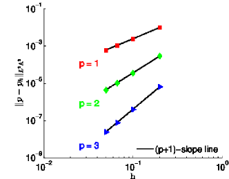
Figure 4: Plots of the $h-$ and $p-$convergence for anisotropic permeability given in (32).

3.2 Layered medium

A classical benchmark for Darcy flow codes is the piecewise constant permeability in a square masud2002stabilized . Such a medium is called layered medium.

$$\mathbb{K}=\begin{bmatrix}\alpha&0\\ 0&\alpha\end{bmatrix}\quad\alpha=\begin{cases}0.3&\text{if $y\leq\frac{1}{3}$}\\ 0.7&\text{if $\frac{1}{3}<y\leq\frac{2}{3}$}\\ 0.5&\text{if $y>\frac{2}{3}$}\end{cases}$$ (35)

The fluid comes into the domain from the left to the right. Since the pressure depends linearly on $x$, horizontal constant velocity is expected in each layer, Figure 5.

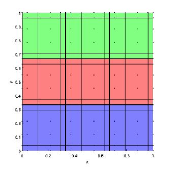
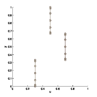
Figure 5: Layered medium with 3 different permeabilities, $\alpha$ ranges top to bottom from $0.5$, $0.7$ and $0.3$. The left figure shows a velocity profile at an arbitrary $x$. Note the numerical solution in the Gauss-Lobatto nodes.

- [1] D. Arnold, R. Falk, and R. Winther. Finite element exterior calculus: from Hodge theory to numerical stability. American Mathematical Society, 47(2):281–354, 2010.
- [2] J. Bonelle and A. Ern. Analysis of compatible discrete operator schemes for elliptic problems on polyhedral meshes. arXiv preprint arXiv:1211.3354, 2012.
- [3] A Bossavit. Discretization of electromagnetic problems. Handbook of numerical analysis, 13:105–197, 2005.
- [4] F Brezzi, A Buffa, and K Lipnikov. Mimetic finite differences for elliptic problems. Mathematical Modelling and Numerical Analysis, 43(2):277–296, 2009.
- [5] W. L. Burke. Applied differential geometry. Cambridge Univ Pr, 1985.
- [6] M. Desbrun, A. Hirani, M. Leok, and J. Marsden. Discrete exterior calculus. Arxiv preprint math/0508341, 2005.
- [7] T. Frankel. The Geometry of Physics. Cambridge University Press, 2nd edition, 2004.
- [8] M Gerritsma. Edge functions for spectral element methods. Spectral and High Order Methods for Partial differential equations, Eds J.S. Hesthaven & E.M. Rønquist, Lecture Notes in Computational Science and Engineering, 76.
- [9] M. Gerritsma, R. Hiemstra, J. Kreeft, A. Palha, P. Pinto Rebelo, and D. Toshniwal. The geometric basis of numerical methods. Proceedings ICOSAHOM 2012 (this issue), 2012.
- [10] R. Herbin and F. Hubert. Benchmark on discretization schemes for anisotropic diffusion problems on general grids. Finite volumes for complex applications V, pages 659–692, 2008.
- [11] R. Hiemstra and M. Gerritsma. High order methods with exact conservation properties. Proceedings ICOSAHOM 2012 (this issue), 2012.
- [12] R. Hiemstra, R. Huijsmans, and M. Gerritsma. High order gradient, curl and divergence conforming spaces, with an application to compatible isogeometric analysis. Submitted to J. Comp Phys., arXiv preprint arXiv:1209.1793, 2012.
- [13] A. Hirani. Discrete Exterior Calculus. PhD thesis, California Institute of Technology, 2003.
- [14] A. Hirani, K. Nakshatrala, and J. Chaudhry. Numerical method for Darcy flow derived using discrete exterior calculus. arXiv preprint arXiv:0810.3434, 2008.
- [15] J. Hyman, M. Shashkov, and S. Steinberg. The numerical solution of diffusion problems in strongly heterogeneous non-isotropic materials. Journal of Computational Physics, 132(1):130–148, 1997.
- [16] J. Kreeft and M. Gerritsma. Higher-order compatible discretization on hexahedrals. Proceedings ICOSAHOM 2012 (this issue), 2012.
- [17] J. Kreeft and M. Gerritsma. Mixed mimetic spectral element method for stokes flow: a pointwise divergence-free solution. Journal of Computational Physics, 2012.
- [18] J. Kreeft and M. Gerritsma. A priori error estimates for compatible spectral discretization of the stokes problem for all admissible boundary conditions. arXiv preprint arXiv:1206.2812, 2012.
- [19] J. Kreeft, A. Palha, and M. Gerritsma. Mimetic framework on curvilinear quadrilaterals of arbitrary order. Submitted to FoCM, Arxiv preprint arXiv:1111.4304, 2011.
- [20] A. Masud and T.J.R. Hughes. A stabilized mixed finite element method for darcy flow. Computer Methods in Applied Mechanics and Engineering, 191(39):4341–4370, 2002.
- [21] A. Palha, P. Pinto Rebelo, and M. Gerritsma. Mimetic spectral element solution for conservative advection. Proceedings ICOSAHOM 2012 (this issue), 2012.
- [22] A. Palha, P. Pinto Rebelo, R. Hiemstra, J. Kreeft, and M. Gerritsma. Physics-compatible discretization techniques on single and dual grids, with application to the Poisson equation of volume forms. Submitted to J. Comp Phys., 2012.
- [23] E Tonti. On the formal structure of physical theories. preprint of the Italian National Research Council, 1975.
- [24] D. Toshniwal, R.H.M. Huijsmans, and M. Gerritsma. A geometric approach towards momentum conservation. Proceedings ICOSAHOM 2012 (this issue), 2012.