Quark scattering off quarks and hadrons

Abstract

The in-medium elastic scattering $qq\to qq,q\bar{q}\to q\bar{q}$ and $\bar{q}\bar{q}\to\bar{q}\bar{q}$ is calculated within the two-flavor Polyakov-loop-extended Nambu-Jona-Lasinio model. The integral and differential quark-quark scattering, its energy and temperature dependence are considered and their flavor dependence is emphasized. The comparison with results of other approaches is presented. The consideration is implemented to the case of quark-pion scattering characterizing the interaction between quarks and hadrons in a kinetic multiphase treatment, and the first estimate of the quark-pion cross sections is given. A possible application of the obtained results to heavy ion collisions is shortly discussed.

, and

1 Introduction

To describe high-energy nuclear physics, the knowledge of the in-medium behavior of quasiparticles such as quarks, gluons, mesons and baryons including their antiparticles is crucial. The quantum chromodynamics (QCD) seems to be the best tool to proceed to this study. Nevertheless, it is well known that the direct implementation of the QCD Lagrangian is not feasible in this state except for some particular cases. In order to avoid the QCD difficulties, some effective models were developed.

In this respect, the low-energy particle sector is well described by effective chiral theories of QCD, the Nambu and Jona-Lasinio (NJL) model [1]. The advantage of this model is that it can be studied in the entire temperature range. The NJL model also offers a simple intuitive view of chiral symmetry breakdown and restoration via the realization of the quark-antiquark pairing similar to the BCS theory of superconductivity. However, a simple point-like interaction form of the model does not ensure its renomalizability, and a cutoff scale $\Lambda$ must be introduced in the theory. The impossibility to treat the confinement-deconfinement phase transition and the absence of gluons are other important defects of the NJL model.

To eliminate partially these defects, it has recently been proposed to couple the quarks to a Polyakov loop [2, 3] as a mechanism that could simulate the confinement, even if the model does not consider the color degrees of freedom as done in QCD. This realized approach is called the Polyakov-Nambu–Jona-Lasinio model (PNJL) [4, 5, 6, 7, 8]. Some recent results show that this approach, exhibiting a smooth crossover at zero baryon density and a first-order phase transition at a large baryon chemical potential, provides some advantages [4, 7]. In particular, the extended model allows one to correctly reproduce lattice data of QCD thermodynamics [5, 9] as well as to improve the NJL model at low temperature due to the suppression of the contribution of colored states. In addition, the PNJL model is more efficient for describing the restoration of the chiral symmetry by a rapid decrease in the effective masses of the quarks [9]. Nevertheless, the phase structure and its dependence on thermodynamic variables is still an open problem and raises some interesting questions including chiral symmetry restoration, color superconductivity, and charged pion condensation phenomena. In particular, it has been found that if the isospin chemical potential $\mu_{I}$ in a charge neutral quark matter is lower than the critical value required for the realization of the pion condensation, pions do not condense and, therefore, even above the critical temperature a bound state with the pion quantum numbers can be formed [10].

At high temperatures ($T>$ 300 MeV) it is supposed that the PNJL description is reliable up to a temperature of approximately 2.5$T_{c}$. For still higher temperatures the transverse gluons, ignored in the PNJL treatment, are expected to be non-negligible [11]. The strong interaction in such a nonperturbative regime of the deconfinement phase is taken into account through an effective temperature-dependent mass for the gluons with a Polyakov-loop background, leaving open the possibility that lighter quasiparticles propagate in the medium [12, 13, 14].

Allowability of quark-gluon degrees of freedom along with hadronic ones means that the model for heavy-ion collisions should be multiphase in nature and include possible phase transitions between different phases. Generally, this complicated situation can be described in terms of hydrodynamics or kinetics which have their own advantages and disadvantages. The use of kinetics for the quark-gluon phase needs knowledge of in-medium cross sections for its constituents. In A MultiPhase Transport (AMPT) model [15] this phase is described in terms of the parton cascade with the partonic elastic cross sections estimated within the perturbative QCD (pQCD). The effect of the surrounding matter was roughly included by introducing the effective Debye mass.

The microscopic quark dynamics is studied in a more elaborated way in the Parton Hadron String Dynamics (PHSD) model [16, 17, 18] where the plasma evolution is solved by a Kadanoff-Baym type equation. Here the potentials between the plasma constituents are chosen in such a way that the model equation of state is consistent with lattice calculations. The cross sections are derived from the spacelike part of the interaction and are employed for the scattering interactions among the plasma constituents. In this model, gluons as well as quarks acquire a large mass when approaching the phase transition. Therefore, the prehadrons which are created in the phase transition are rather heavy. Another model which allows for these studies is a gluonic cascade realized in the Boltzmann Approach to Multi Parton Scattering (BAMPS) [19]. The gluon emission and interaction during the expansion stage of the QGP move the system towards equilibrium. A parton cascade approach with a pQCD inspired cross section was applied also at the RHIC energy to study scaling properties of the elliptic flow [20] and ’chemical’ composition of the quark-gluon plasma [21].

The quantum molecular dynamics of the expanding $q/\bar{q}$ plasma has been proposed recently [22]. Properties of quarks as well as elastic scattering cross sections were calculated within the three-flavor NJL model.

All the kinetic multiphase models mentioned above should describe a transition from one to another phase: from quarks-gluons to hadrons, in our case. This smooth transition is simulated by a possible coalescence of quark-antiquark or three quarks, being close to each other in coordinate and momentum space, to form a meson or a baryon thereby creating a mixed parton-hadron phase which is a typical feature of the crossover phase transition. As was demonstrated in Ref. [23] in terms of a simple thermodynamically consistent statistical model, the gluon-glueball system exhibiting a crossover phase transition shows the first order phase transition if the interaction between mixed phase constituents is neglected. As to chiral NJL-like models, the appearance of a first-order chiral phase transition is a characteristic feature of the simplest versions of these models. Sensitivity of the phase structure to the parameters characterizing the quasiparticle interaction has noted many years ago. In particular, it was shown that the location of the QCD critical point moves in accord with the repulsive vector-channel interaction which may result in the disappearance of the critical end-point at sufficiently large values of the vector interaction coupling turning it into crossover [24, 25, 26, 27]. A pronounced impact on the phase diagram is also given by breaking of the $U(1)$ symmetry due to the axial anomaly in QCD which is introduced into models by adding the Kobayashi-Maskava-’t Hooft interaction to be responsible for the large mass of the $\eta^{\prime}$ meson. The decrease of this interaction strength may dismiss the associated existence of a critical point in the phase diagram [25, 27].

In this work, we want to make a step towards account for the interaction between constituents of quark-gluon and hadronic phases. Basing on the PNJL model we give here the first estimate for interaction of quarks/antiquarks with pions which is expected to be a dominant component of this type of interactions.

Thus, the purpose of this paper is to calculate quark-quark, quark-antiquark and antiquark-antiquark cross sections and generalize this approach to the case of quark-pion scattering. The consideration is based on the chiral two-flavor PNJL model the key points of which are remind in the next Section II. In Sections III and IV, the main equations are given for different channels of quark-(anti)quark elastic scattering and are generalized to the quark-hadron case in Section IV. Their numerical results for the $qq$ and $qH$ processes are presented and discussed in Section V. We conclude the obtained results in Section VI.

2 The PNJL model used

The deconfinement in a pure $SU_{f}(2)$ gauge theory can be simulated by introducing a complex Polyakov loop field. The two-flavor PNJL model is used with the following Lagrangian [5, 28, 29] :

$$\mathcal{L}_{\rm PNJL}=\bar{q}\left(i\gamma_{\mu}D^{\mu}-\hat{m}_{0}\right)q+G\left[\left(\bar{q}q\right)^{2}+\left(\bar{q}i\gamma_{5}\vec{\tau}q\right)^{2}\right]-\mathcal{U}\left(\Phi[A],\bar{\Phi}[A];T\right)~{},$$ (1)

where scalar and pseudoscalar interactions are taken into account, $G$ is the coupling constant, $\vec{\tau}$ is the Pauli matrix in the flavor space, $\bar{q}$ and $q$ are the quark fields (color and flavor indices are suppressed), $\hat{m}_{0}$ is the diagonal matrix of the current quark mass, $\hat{m}_{0}=\mbox{diag}\,(m^{0}_{u},m^{0}_{d})$ and $m^{0}_{u}=m^{0}_{d}=m_{0}$. The vectorial and axial interaction terms are neglected in Eq. (1).

The quark fields are related to the gauge field $A^{\mu}$ through the covariant derivative $D^{\mu}=\partial^{\mu}-iA^{\mu}$, where the gauge field is $A^{\mu}=\delta_{0}^{\mu}A^{0}=-i\delta_{4}^{\mu}A_{4}$ (the Polyakov calibration). The field $\Phi$ is determined by tracing the Polyakov loop $L(\vec{x})$ [5]: $\Phi[A]=\frac{1}{N_{c}}\mbox{Tr}_{c}L(\vec{x})$, where $L(\vec{x})=\mathcal{P}\exp\left[\displaystyle i\int_{0}^{\beta}d\tau A_{4}(\vec{x},\tau)\right]$.

The gauge sector of the Lagrangian density (1) is described by an effective potential $\mathcal{U}\left(\Phi[A],\bar{\Phi}[A];T\right)$ fitted to lattice QCD simulation results in a pure $SU(3)$ gauge theory at finite $T$ [5, 30]

$$\frac{\mathcal{U}\left(\Phi,\bar{\Phi};T\right)}{T^{4}} = -\frac{b_{2}\left(T\right)}{2}\bar{\Phi}\Phi-\frac{b_{3}}{6}\left(\Phi^{3}+{\bar{\Phi}}^{3}\right)+\frac{b_{4}}{4}\left(\bar{\Phi}\Phi\right)^{2}$$ (2)

$$b_{2}\left(T\right) = a_{0}+a_{1}\left(\frac{T_{0}}{T}\right)+a_{2}\left(\frac{T_{0}}{T}\right)^{2}+a_{3}\left(\frac{T_{0}}{T}\right)^{3}~{}.$$ (3)

The parameters of the effective potential (2) and (3) defined by fitting to the lattice results are summarized in [36] with the model parameter value of $T_{0}=0.19$ GeV.

The grand potential for the PNJL theory in the mean-field approximation is given by the following equation [29] :

$$\Omega(\Phi,\bar{\Phi},m,T,\mu) = \mathcal{U}\left(\Phi,\bar{\Phi};T\right)+G\langle\bar{q}q\rangle^{2}+\Omega_{q}$$ (4)

where

$$\Omega_{q}=-2N_{c}N_{f}\int\frac{d^{3}p}{(2\pi)^{3}}E_{p}-2N_{f}T\int\frac{d^{3}p}{(2\pi)^{3}}\left[\ln N_{\Phi}^{+}(E_{p})+\ln N_{\Phi}^{-}(E_{p})\right]~{},$$

$E_{p}$ is the quark energy, $E_{p}=\sqrt{{\bf p}^{2}+m^{2}}$, $E_{p}^{\pm}=E_{p}\mp\mu$ ($\mu$ is the chemical potential) and $N_{\Phi}^{\pm}(E_{p})$ is the partition density with

$$N_{\Phi}^{+}(E_{p})=\left[1+3\left(\Phi+\bar{\Phi}e^{-\beta E_{p}^{+}}\right)e^{-\beta E_{p}^{+}}+e^{-3\beta E_{p}^{+}}\right]^{-1},$$

(5)

$$N_{\Phi}^{-}(E_{p})=\left[1+3\left(\bar{\Phi}+{\Phi}e^{-\beta E_{p}^{-}}\right)e^{-\beta E_{p}^{-}}+e^{-3\beta E_{p}^{-}}\right]^{-1}.$$

The gap equation for the constituent quark mass is obtained by solving the equation ${\partial\Omega(\Phi,\bar{\Phi},m,T,\mu)}/{\partial m}=0$ with the grand potential (4):

$$m=m_{0}-N_{f}G<{\bar{q}}q>=m_{0}+8GN_{c}N_{f}\int_{\Lambda}\frac{d^{3}p}{(2\pi)^{3}}\frac{m}{E_{p}}\left[1-f^{+}_{\Phi}-f^{-}_{\Phi}\right]~{},$$ (6)

where $f_{\Phi}^{+}$, $f_{\Phi}^{-}$ are the modified Fermi functions

$$f_{\Phi}^{+}=((\Phi+2\bar{\Phi}e^{-\beta E^{+}})e^{-\beta E^{+}}+e^{-3\beta E^{+}})N_{\Phi}^{+},$$

(7)

$$f_{\Phi}^{-}=((\bar{\Phi}+2{\Phi}e^{-\beta E^{-}})e^{-\beta E^{-}}+e^{-3\beta E^{-}})N_{\Phi}^{-}$$

and $\beta=1/T$ is the inverse temperature.

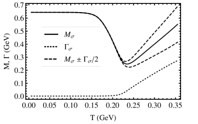
Figure 1: Meson mass $M_{\pi/\sigma}\pm\Gamma_{\pi/\sigma}/2$, the double quark mass and the meson width $\Gamma_{\pi/\sigma}$ in the PNJL model.

In our model, the mesons as $q-\bar{q}$ bound states are constructed by the quark-antiquark interaction within the random-phase approximation [31]. It leads to the explicit form for the meson propagators

$$D_{\pi/\sigma}(k_{0},{\bf k})=\dfrac{G}{1-2G\Pi_{\pi/\sigma}(k_{0},{\bf k})}.$$ (8)

In the self-consistent Hartree limit masses of bound states are determined as poles of the meson propagators in the random-phase approximation. Therefore, the $\pi$ and $\sigma$ meson masses are the solutions of the equation

$$1-2G\ \Pi_{{\pi/\sigma}}(k_{0},{\bf k})=0,$$ (9)

where $k^{2}=M^{2}_{\pi}$ and $k^{2}=M^{2}_{\sigma}$ in pseudoscalar and scalar sectors, respectively, and $\Pi_{{\pi}/{\sigma}}$ are the correlation functions with the quark propagator $S_{\pi/\sigma}(k)$ [31]

$$i\Pi_{\pi}(k^{2})=\int\frac{d^{4}p}{(2\pi)^{4}}\ \mbox{Tr}\,\left[i\gamma_{5}\tau^{a}S_{\pi}(p+k)i\gamma_{5}\tau^{b}S_{\pi}(p)\right],$$ (10)

$$i\Pi_{\sigma}(k^{2})=\int\frac{d^{4}p}{(2\pi)^{4}}\ \mbox{Tr}\,\left[iS_{\sigma}(p+k)iS_{\sigma}(p)\right].$$ (11)

Equation (9) means that in the pole approximation to be reasonable in the $1/N_{c}$ consideration, the meson propagators $D_{\pi/\sigma}$ can be written as

$$D_{\pi/\sigma}(k_{0},{\bf k})=\dfrac{G}{1-2G\Pi_{\pi/\sigma}(k_{0},{\bf k})}\approx\dfrac{g^{2}_{\pi q\bar{q}/\sigma q\bar{q}}}{k^{2}-M_{\pi/\sigma}^{2}}.$$ (12)

As in Refs. [31]-[35], both the pion-quark $g_{\pi q\bar{q}}(T,\mu)$ and sigma-quark $g_{\sigma q\bar{q}}(T,\mu)$ coupling strengths can be obtained now from $\Pi_{{\pi}/{\sigma}}$ :

$$g_{\pi q\bar{q}/\sigma q\bar{q}}^{-2}(T,\mu)=\frac{\partial\Pi_{{\pi}/{\sigma}}(k^{2})}{\partial k^{2}}|_{{}^{k^{2}=m_{\pi}^{2}}_{k^{2}=m_{\sigma}^{2}}}.$$ (13)

The regularization parameter $\Lambda$, the quark current mass $m_{0}$, the coupling strength G, the parameter $T_{0}$ and the Mott temperature in these calculations are presented in Table 1. In the PNJL model there are two critical temperatures: The critical temperature of the chiral transition and the deconfinement temperature which can coincide for some model parameter set [36]. The first quantity is obtained as a minimum of $\partial m/\partial T$ and the second one as a maximum of $\partial\Phi/\partial T$. For the vanishing chemical potential the temperature of the chiral transition is $T_{c}=$0.210 GeV for our model parameters.

Table 1: The model parameters

$m_{0}$ [MeV]	$\Lambda$ [GeV]	$G$ [GeV]-2	$T_{0}$ [GeV]	$T_{\rm Mott}$ [GeV]
5.5	0.639	5.227	0.19	0.231

The temperature dependence of $\pi$ and $\sigma$-meson masses is shown in Fig. 1, its behavior is typical for NJL-like models. The double mass of constituent quarks $2m$ is also plotted in this figure. As is seen, the curve for $2m$ crosses the $\pi$-meson one at $T=$0.231 GeV allowing the pion to dissociate into their constituents. This so-called Mott temperature is sometimes considered as a ”soft” form of deconfinement. Note that $T_{Mott}>T_{c}$. At higher temperatures both scalar and pseudoscalar meson masses jointly increase. The decay width of $\pi$ and $\sigma$ mesons, $\Gamma_{\pi}$ and $\Gamma_{\sigma}$, monotonically grows above the Mott temperature as $T$ increases.

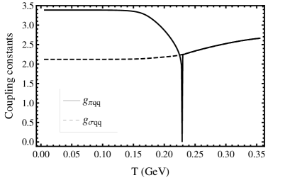
Figure 2: Coupling constants $g_{\sigma qq}$ (dashed line) and $g_{\pi qq}$ (solid line).

As demonstrated in Fig. 2 and in accordance with Eq. (13), the quark-$\sigma$ coupling constant is rather weakly sensitive to the temperature slowly increasing with $T$ but in the quark-pion case the coupling constant exhibits a kink singularity just at the Mott temperature. Technically, this feature results in the coupling strengths approaching zero for $T\to T_{Mott}$ from below. This behavior differs markedly from the behavior of the couplings when evaluated in the chiral limit.

3 Scattering cross section for the $qq\rightarrow qq$ and $q\overline{q}\rightarrow q\overline{q}$ processes

Quark-quark elastic scattering

Let us consider now the quark scattering processes. The amplitude of the quark-quark scattering to $1/N_{c}$ order is given by two diagrams presented in Fig. 3 with taking into account the channels with pion and $\sigma$-meson creation in an intermediate state:

$$-iT_{t} = \overline{u}(q_{3})\Gamma_{\pi}u(q_{1})\frac{1}{(q_{1}-q_{3})^{2}-M_{\pi}^{2}}\overline{u}(q_{4})\Gamma_{\pi}u(q_{2})+$$ (14)

$$\overline{u}(q_{3})\Gamma_{\sigma}u(q_{1})\frac{1}{(q_{1}-q_{3})^{2}-M_{\sigma}^{2}}\overline{u}(q_{4})\Gamma_{\sigma}u(q_{2}),$$

$$-iT_{u} = \overline{u}(q_{4})\Gamma_{\pi}u(q_{1})\frac{1}{(q_{1}-q_{4})^{2}-M_{\pi}^{2}}\overline{u}(q_{3})\Gamma_{\pi}u(q_{2})+$$ (15)

$$\overline{u}(q_{4})\Gamma_{\sigma}u(q_{1})\frac{1}{(q_{1}-q_{4})^{2}-M_{\sigma}^{2}}\overline{u}(q_{3})\Gamma_{\sigma}u(q_{2}),$$

where $\Gamma_{\pi}=(i\gamma_{5})\cdot g_{\pi qq}$ and $\Gamma_{\sigma}={\bf 1}\cdot g_{\sigma qq}$. Here $s$ and $t$ are the usual Mandelstam variables. After appropriate transformations and bearing in mind that the total quark-quark amplitude is $\displaystyle T_{qq}=\dfrac{1}{4N_{c}^{2}}\sum_{c}|T_{t}+T_{u}|^{2}$ we get the following result :

$$|T_{t}|^{2} = \left(|D_{t}^{\sigma}|^{2}(t-4m^{2})^{2}+|D_{t}^{\pi}|^{2}t^{2}\right),$$ (16)

$$|T_{u}|^{2} = \left(|D_{u}^{\sigma}|^{2}(u-4m^{2})^{2}+|D_{u}^{\pi}|^{2}u^{2}\right),$$ (17)

$$T_{t}T^{*}_{u} = -\frac{1}{2N_{c}}(D_{t}^{\sigma}D_{u}^{\sigma}(tu+4m^{2}(u+t)-16m^{2})-D_{t}^{\sigma}D_{u}^{\pi}u(t-4m^{2})$$ (18)

$$- D_{t}^{\pi}D_{u}^{\sigma}t(u-4m^{2})+D_{t}^{\pi}D_{u}^{\pi}tu)~{},$$

where the effective meson propagators in the $t$ and $u$ channels are

$$D^{\sigma/\pi}_{t}=\frac{g^{2}_{\sigma qq/\pi qq}}{t-M_{\sigma/\pi}^{2}},\ \ \ D^{\sigma/\pi}_{u}=\frac{g^{2}_{\sigma qq/\pi qq}}{u-M_{\sigma/\pi}^{2}}~{}.$$ (19)

with the coupling constants $g_{\sigma qq\ \pi qq}$ defined from Eq. (13).

         

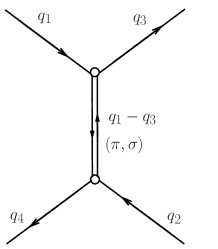
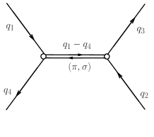
Figure 3: Diagrams of $qq\rightarrow qq$ for $t$-channel (left) and $u$-channel (right)

The differential cross section has the form

$$\frac{d\sigma_{el}}{dt}=\frac{|T|^{2}}{16\pi\lambda(s,m^{2})}$$ (20)

with $\lambda(s,m^{2})=(s-4m^{2})s$.

Then the total cross section of the $qq\rightarrow qq$ and $q\overline{q}\rightarrow q\overline{q}$ elastic scattering is:

$$\sigma_{\rm el}=\frac{1}{16\pi\lambda(s,m^{2})}\int^{t^{+}}_{t{-}}{dt\ |T|^{2}}\ (1-f_{\Phi}(\frac{\sqrt{s}}{2}\mp\mu))\ (1-f_{\Phi}(\frac{\sqrt{s}}{2}\mp\mu))~{},$$ (21)

where the inserted blocking factors $(1-f_{\Phi})$ take into account that rescattered particles appear in a medium where other identical particles have already existed. Here $f_{\Phi}(\sqrt{s}/2\mp\mu)\to f^{\mp}_{\Phi}$ is the modified Fermi function (7) and the sign in front of the chemical potential $\mu$ corresponds to a particle or an antiparticle. The integration limits in Eq. (21) for the $qq$ case of equal masses are $t^{+}=0$ and $t^{-}=4m^{2}-s$. The kinematic boundary reads $s>4m^{2}$.

For calculation of the differential cross section in the center-of-mass system it can be rewritten in the Mandelstam variables as $t=-2{p^{*}}^{2}(1-{\rm cos}\Theta)$ and $u=-2{p^{*}}^{2}(1+{\rm cos}\Theta)$, where in the center-of-mass system we have

$$p^{*}=q^{*}_{1}=q^{*}_{2}=q^{*}_{3}=q^{*}_{4}=\frac{\lambda^{1/2}(s,m^{2},m^{2})}{2\sqrt{s}}.$$ (22)

It is easy to show that the scattering amplitude for the process $q\overline{q}\rightarrow q\overline{q}$ can be obtained from the expressions for the process $qq\rightarrow qq$ by the substitution $t\leftrightarrow t$, $s\leftrightarrow u$ , $u\leftrightarrow s$. The total elastic scattering amplitude for $\overline{q}\ \overline{q}\rightarrow\overline{q}\ \overline{q}$ follows immediately from the $qq\to qq$ amplitude by time reversal invariance, as long as no chemical potential is involved.

Quark-antiquark elastic scattering

Diagrams for the quark-antiquark process, $q\overline{q}\rightarrow q\overline{q}$, are given in Fig. 4.

         

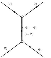
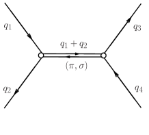
Figure 4: Diagrams of $q\bar{q}\rightarrow q\bar{q}$ for $t$-channel (left) and $s$-channel (right)

Similarly to the quark-quark case we have for the $q\bar{q}$ scattering

$$|T_{t}|^{2} = \left(|D_{t}^{\sigma}|^{2}(t-4m^{2})^{2}+|D_{t}^{\pi}|^{2}t^{2}\right),$$ (23)

$$|T_{s}|^{2} = \left(|D_{s}^{\sigma}|^{2}(s-4m^{2})^{2}+|D_{s}^{\pi}|^{2}s^{2}\right),$$ (24)

$$T_{t}T^{*}_{s} = -\frac{1}{2N_{c}}(D_{t}^{\sigma}D_{s}^{\sigma}(ts+4m^{2}(s+t)-16m^{2})-D_{t}^{\sigma}D_{s}^{\pi}s(t-4m^{2})$$ (25)

$$- D_{t}^{\pi}D_{s}^{\sigma}t(s-4m^{2})+D_{t}^{\pi}D_{s}^{\pi}ts)$$

with the meson propagators

$$D^{\sigma/\pi}_{t}=\frac{g^{2}_{\sigma qq/\pi qq}}{t-M_{\sigma/\pi}^{2}},\ \ \ D^{\sigma/\pi}_{s}=\frac{g^{2}_{\sigma qq/\pi qq}}{s-M_{\sigma/\pi}^{2}},$$ (26)

where we use the pole approximation for meson propagators.

Taking into consideration the isospin factors we can consider the following independent types of scattering reactions for quark-quark scattering :

$$uu\rightarrow uu\ \ (dd\rightarrow dd),$$

(27)

$$ud\rightarrow ud\ \ (du\rightarrow du),$$

where the first of them includes both $t$ and $u$ channels and the second includes only the $u$-channel. In the same way, for quark-antiquark scattering we have a similar relation:

$$u\bar{u}\rightarrow u\bar{u}\ \ (d\bar{d}\rightarrow d\bar{d}),$$

$$u\bar{d}\rightarrow u\bar{d}\ \ (d\bar{u}\rightarrow d\bar{u}),$$ (28)

$$u\bar{u}\rightarrow d\bar{d}$$

with both $t$ and $s$ channels for the first reaction, the $t$-channel for the second one and the $s$-channel for the third one, respectively.

The total and differential cross sections for antiquark-antiquark coincide with those for quark-quark scattering and can be calculated as in Eqs. (20), (21).

4 Amplitudes for the $qH\longrightarrow qH$ process

The Feynman diagrams for calculation of the quark-pion scattering amplitudes with the exchange of a quark, $\pi$- and $\sigma$-meson are shown in Fig. 5.

           

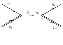
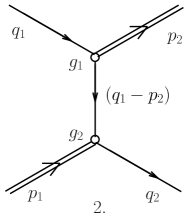
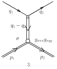
Figure 5: The Feynman diagrams for the $s-$ and $u-$quark exchange channels (diagrams 1 and 2) and the t-channel with the exchange by the sigma-meson (diagram 3). The double line corresponds to a pion.

The amplitude in the $s$-channel (diagram 1 in Fig. 5) is as follows:

$$-iT_{1} = \overline{u}({\bf q_{2}})g_{2}(i\gamma_{5})\frac{((\widehat{q}_{1}+\widehat{p}_{1})+m)}{s-m^{2}}(i\gamma_{5})g_{1}u({\bf q_{1}}),$$

$$iT^{*}_{1} = u({\bf q_{2}})g_{2}(i\gamma_{5})\gamma_{0}\frac{((\widehat{q}_{1}+\widehat{p}_{1})+m)^{\dagger}}{s-m^{2}}\gamma_{0}(i\gamma_{5})g_{1}\overline{u}({\bf q_{1}})~{}.$$

After the transformation, Eq. (4) reads

$$iT^{*}_{1} = -iu({\bf q_{2}})g_{2}(i\gamma_{5})\frac{((\widehat{q}_{1}+\widehat{p}_{1})+m)}{s-m^{2}}(i\gamma_{5})g_{1}\overline{u}({\bf q_{1}})~{}.$$ (30)

The result for the $u$-channel can be obtained by the substitution $p_{1}\rightarrow-p_{2}$

$$-iT_{2} = \overline{u}({\bf q_{2}})g_{2}(i\gamma_{5})\frac{((\widehat{q}_{1}-\widehat{p}_{2})+m)}{u-m^{2}}(i\gamma_{5})g_{1}u({\bf q_{1}}),$$

$$iT^{*}_{2} = u({\bf q_{2}})g_{2}(i\gamma_{5})\frac{((\widehat{q}_{1}-\widehat{p}_{2})+m)}{u-m^{2}}(i\gamma_{5})g_{1}\overline{u}({\bf q_{1}}).$$

The amplitude of the process with the $\sigma$-meson exchange is as follows :

$$-iT_{3} = \overline{u}(q_{2}){\bf 1}u(q_{2})\frac{1}{t-M^{2}_{\sigma}}g_{\sigma\pi\pi}g_{\sigma qq},$$

$$iT^{*}_{3} = \overline{u}(q_{2})(\gamma_{0}{\bf 1}\gamma_{0})u(q_{2})\frac{1}{t-M^{2}_{\sigma}}g_{\sigma\pi\pi}g_{\sigma qq}.$$

The total amplitude of the process is given as $\displaystyle|T|^{2}=f_{c}\sum_{c}|T_{1}+T_{2}+T_{3}|^{2}$ and then after tracing and transforming equations we get:

$$T_{1}T^{*}_{1} = N_{c}K_{s}^{2}[M_{\pi}^{4}-(s-m^{2})(u-m^{2})],$$ (33)

$$T_{1}T^{*}_{2} = T_{2}T^{*}_{1}=N_{c}K_{s}K_{u}[-M_{\pi}^{4}+(s-m^{2})(u-m^{2})],$$ (34)

$$T_{1}T^{*}_{3} = T_{3}T^{*}_{1}=N_{c}K_{s}K_{t}[m(s-u)],$$ (35)

$$T_{2}T^{*}_{2} = N_{c}K_{u}^{2}[M_{\pi}^{4}-(s-m^{2})(u-m^{2})],$$ (36)

$$T_{3}T^{*}_{2} = T_{2}T^{*}_{3}=-N_{c}K_{u}K_{t}[m(s-u)],$$ (37)

$$T_{3}T^{*}_{3} = N_{c}K_{t}^{2}(4m^{2}-t)~{},$$ (38)

where $m,M_{\pi},M_{\sigma}$ are the masses of the quark, pion and sigma-meson, respectively. Summation is carried over color and the type of reacton.

Here we have introduced the propagators $K_{s},K_{u},K_{t}$

$$K_{s}=\frac{g^{2}_{\pi qq}}{s-m^{2}},\ \ \ K_{u}=\frac{g^{2}_{\pi qq}}{u-m^{2}},\ \ \ K_{t}=\frac{g_{\sigma\pi\pi}g_{\sigma qq}}{t-M^{2}_{\sigma}},$$ (39)

where $g_{\pi qq}$, $g_{\sigma qq}$ are defined by Eq. (13) and the coupling strength of $\sigma-\pi\pi$ is interrelated as $g_{\sigma\pi\pi}=2g_{\sigma qq}g^{2}_{\pi qq}A_{\sigma\pi\pi}$ and $A_{\sigma\pi\pi}$ is the amplitude of the $\sigma\rightarrow\pi\pi$ decay [32]. Summation over colors depends on the reaction type. Taking into account the diagrams with $1/N_{c}$ and $1/N_{c}^{2}$ corrections we have got color factors $f_{c}$. Both color and flavor factors for each reaction are given in Table 2.

Table 2: Flavor and color structure of the processes

Process	Isospin factor	color factor $f_{c}$
$\rm{u}\pi^{0}\rightarrow\rm{u}\pi^{0}$	$\frac{1}{2}K_{s}$, $\frac{1}{2}K_{u}$ , $K_{t}$	$\left(1+\frac{2}{N_{c}}+\frac{1}{N_{c}^{2}}\right)$
$\rightarrow\rm{d}\pi^{+}$	$\frac{1}{\sqrt{2}}K_{s}$, $\frac{1}{\sqrt{2}}K_{u}$, $K_{t}$	$\left(1+\frac{1}{N_{c}}\right)$
$\rm{u}\pi^{-}\rightarrow\rm{u}\pi^{-}$	$K_{s}$, $K_{u}$, $K_{t}$	$\left(1+\frac{1}{N^{2}_{c}}\right)$
$\rightarrow\rm{d}\pi^{0}$	$\frac{1}{\sqrt{2}}K_{s}$, $\frac{1}{\sqrt{2}}K_{u}$, $K_{t}$	$\left(1+\frac{1}{N_{c}}\right)$
$\rm{d}\pi^{0}\longrightarrow\rm{d}\pi^{0}$	$\frac{1}{2}K_{s}$, $\frac{1}{2}K_{u}$, $K_{t}$	$\left(1+\frac{2}{N_{c}}+\frac{1}{N_{c}^{2}}\right)$
$\rightarrow\rm{u}\pi^{-}$	$\frac{1}{\sqrt{2}}K_{s}$,  $\frac{1}{\sqrt{2}}K_{u}$, $K_{t}$	$\left(1+\frac{1}{N_{c}}\right)$
$\rm{d}\pi^{+}\longrightarrow\rm{d}\pi^{+}$	$K_{s}$, $K_{u}$, $K_{t}$	$\left(1+\frac{1}{N^{2}_{c}}\right)$
$\rightarrow\rm{u}\pi^{0}$	$\frac{1}{\sqrt{2}}K_{s}$, $\frac{1}{\sqrt{2}}K_{u}$, $K_{t}$	$\left(1+\frac{1}{N_{c}}\right)$

Kinematic invariants for the $qH\rightarrow qH$ scattering process are defined as follows:

$$s=(q_{1}+p_{1})^{2}=(q_{2}+p_{2})^{2},$$

$$t=(q_{1}-q_{2})^{2}=(p_{1}-p_{2})^{2},$$

(40)

$$u=(q_{1}-p_{2})^{2}=(q_{2}-p_{1})^{2},$$

$$s+t+u=2M_{\pi}^{2}+2m^{2}.$$

The differential cross section has the form similar to Eq. (20)

$$\frac{d\sigma_{el}}{dt}=\frac{|T|^{2}}{16\pi\lambda(s,m^{2},M_{\pi}^{2})}$$ (41)

with $\lambda(s,m^{2},M_{\pi}^{2})=(s-(M_{\pi}+m)^{2})(s-(M_{\pi}-m)^{2})$. Accordingly, the integrated cross section for the elastic $qH$ scattering is:

$$\sigma_{\rm el}=\frac{1}{16\pi\lambda(s,m^{2},M_{\pi}^{2})}\int^{t^{+}}_{t{-}}{dt\ |T|^{2}}(1-f_{\Phi}(E_{q}\mp\mu))\ (1+f_{B}(E_{H}\mp\mu))~{},$$ (42)

where $E_{q}$, $E_{H}$ correspond to the quark and hadron energies, the Bose-Einstein factor has the form $f_{B}=(\exp(\beta x)-1)^{-1}$ and the integration limits are

$$t^{\pm}=2m^{2}-\frac{1}{2s}\left\{(s+m^{2}-M_{\pi}^{2})^{2}\mp\lambda(s,m^{2},M_{\pi}^{2})\right\}.$$ (43)

As follows from Eq. (42) for the cross section, the $q\pi$ reaction has kinematic boundaries $s>{\rm max}\left\{(m+M_{\pi})^{2},(m-M_{\pi})^{2}\right\}$.

For calculation of the differential cross section in the center-of-mass system we can use the same expressions as for the $qq$-scattering keeping in mind that ${p^{*}}^{2}$ differs from Eq. (22) because the $\lambda(s,m^{2},M_{\pi}^{2})$ factor has a different form.

5 Numerical results and discussion

Quark-(anti)quark elastic cross-section

We shall start with the PNJL calculation of the in-medium $qq,q\bar{q}$ and $\bar{q}\bar{q}$ cross sections. The integral cross sections $\sigma_{el}$ are plotted in Fig. 6 for various types of reactions shown in Eqs. (3),(3). A strict limit of the applicability of the quark model at high energies is not well established. As mentioned in work [33], the center-of-mass energy $\sqrt{s}$ in our model is restricted by the scale $\sqrt{s}=2\sqrt{\Lambda^{2}+m_{q}^{2}}\approx$ 1.5 GeV.

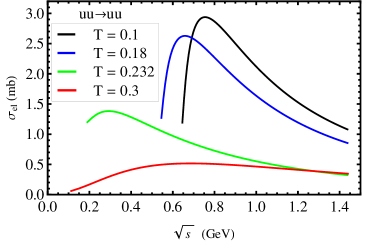
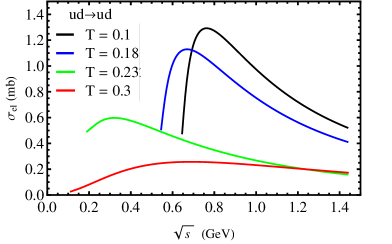
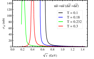
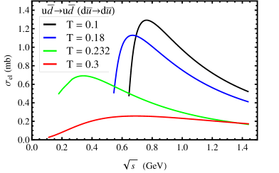
Figure 6: Total cross section of reactions $qq\rightarrow qq$ (two upper plots) and $q\bar{q}\rightarrow q\bar{q}$ (two bottom plots) at different temperatures.

The quark scattering cross sections are relatively featureless. For quark-quark scattering the flavor influences mainly the magnitude of the cross sections, being larger for quarks of the same flavors ($\sigma_{el}(uu\to uu)\approx 2.5\sigma_{el}(ud\to ud)$) (compare two upper panels in Fig. 6). This is because the $ud$ scattering has in fact less exchange mesons available in the $u$-channel, since no neutral particles are admissible in this channel. The energy dependence of $\sigma_{el}$ is very similar in both cases: the cross section has a clear maximum at the energy $\sqrt{s}\sim$1 GeV for a moderate temperature $T\sim$ 0.1 GeV which moves to smaller $\sqrt{s}$ as temperature increases exhibiting almost singular behavior at $T=T_{Mott}$. As noted in Introduction, the PNJL model is reliable for temperatures $T\stackrel{{\scriptstyle\scriptstyle<}}{{\phantom{}{}_{\sim}}}2.5T_{c}$ [11] where for our 2-flavor model we have $T_{c}\approx 0.5(T_{0}+T_{Mott})=$210 MeV (see Tabl 1). The $\sigma_{el}$ is getting rather flat if the temperature exceeds the Mott temperature (see the case $T=$ 0.3 GeV in Fig. 6).

Note that the cross section is evaluated according to Eq. (21,) where the modified Pauli factor for scattered quarks is involved. As is seen from Fig. 6, $\sigma_{el}$ decreases when $\sqrt{s}$ grows, which is a consequence of nonperturbativity in the coupling constant $G$ of the PNJL treatment. In the Born approximation the opposite behavior $\sigma_{el}\sim s$ is observed, as was demonstrated in Ref. [34]. The behavior of the scattering cross section for quark-antiquark of different types is very close to that for quark-quark of different flavors (compare $ud$ and $u\bar{d}$ reactions in Fig. 6). However, for quark-antiquark of the same flavor ($u\bar{u}$ and $d\bar{d}$) the cross section at any temperature has the resonance-dominated behavior demonstrating a huge maximum located at the energy close to the $\sigma$-meson mass. In other words, the quark-antiquark scattering shows a threshold divergence at the Mott temperature $T_{Mott}$, at which the pion dissociates into its constituents and becomes a resonant state. This feature manifests itself in other processes like $q\bar{q}\to\gamma\gamma$ [37] as well as $\pi\pi\to\pi\pi$ [32, 38] and $\pi\gamma\to\pi\gamma$ [39]. The dramatically high cross sections mean that near $T_{Mott}$ a local equilibrium can be established.

Figure 7: Comparison of the energy dependence of the elastic cross section for the $uu\rightarrow uu$ scattering for a temperature above the Mott temperature. The dotted and dashed lines are the NJL results for $SU_{f}(3)$ and $SU_{f}(2)$, respectively, from Refs. [35, 34], the solid line is our two-flavor PNJL calculations for $T=$ 0.27 GeV.

The calculated results can be compared with those obtained earlier [34, 33]. Some elastic scattering cross sections were calculated in the two-flavor sector $SU_{f}(2)$ of the NJL model with the additional restriction of the chiral limit condition $m=$0 in Ref. [34]. The three flavor NJL model was considered in [33] and the results are exemplified in Fig. 7. It is seen that the $SU_{f}(3)$ calculation yields a larger cross section for $uu\rightarrow uu$ than the corresponding two-flavor case. This is due to the point that the additional exchange channels $\eta,\eta^{\prime}$ and $\sigma^{\prime}$ are missing in the two flavor case. In particular, the $uu\to uu$ channel of the elastic scattering at $T=0.215$ GeV for $SU_{f}(3)$ is regularly above that for $SU_{f}(2)$ by the factor of (3-4) in the whole energy range from the threshold till $\sqrt{s}\sim$1.2 GeV [33] (compare two dotted lines in Fig. 7). The values of the $uu\to uu$ cross section for $SU_{f}(2)$ [33] with $T_{Mott}$ are consistent with our PNJL results presented in Fig. 7 if one takes into account the different Mott temperatures in these calculations. It is not surprising since the suppression due to the Polyakov loop works only in the low temperature sector, $T<T_{Mott}$.

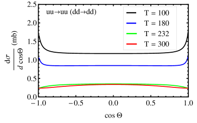
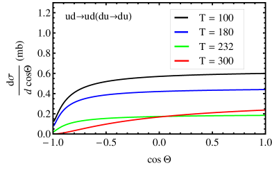
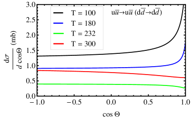
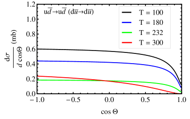
Figure 8: Angular distribution of the elastic scattering processes $qq\rightarrow qq$ (upper panels) and $q\bar{q}\rightarrow q\bar{q}$ (bottom panels) at $\sqrt{s}=1$ GeV for different temperatures.

For each process the differential cross sections may also be calculated. As an example, the angular distribution in the elastic $qq$ and $q\bar{q}$ scatterings is presented in Fig. 8 at the energy $\sqrt{s}=$1 GeV. In the case of quarks of the same flavors ($uu$), the angular distribution is isotropic except for the narrow region $|cos\Theta|\stackrel{{\scriptstyle\scriptstyle>}}{{\phantom{}{}_{\sim}}}$0.9. The differential distributions for quarks of various flavors ($ud$) or different types ($u\bar{d})$ are also almost flat, besides the region $|cos\Theta|\stackrel{{\scriptstyle\scriptstyle>}}{{\phantom{}{}_{\sim}}}$0.8, but this deflection from isotropy is in the backward direction for the $ud$ while it is in the forward direction for $u\bar{d}$ reactions. For the $u\bar{u}$ and the $d\bar{d}$ scatterings, the angular distribution changes from isotropic to clearly anisotropic one if the temperature decreases from $T_{Mott}$ to about 0.1 GeV. In accordance with the temperature dependence of $\sigma_{el}$, the magnitude of the differential distribution of $d\sigma_{el}/dcos\Theta$ decreases with the growth of the temperature.

The processes presented in Figs. 3 and 4 can also be calculated in the lowest order perturbative QCD. These on-shell high-energy calculations are in use starting from the first classical parton cascade model [40]. In Fig. 9, the comparison between the PNJL and the pQCD results (obtained according to the model description in Appendix of Ref. [34]) is given. As is seen, in contrast with the PNJL, the pQCD description predicts a strong scattering enhancement at forward angles for finite parton masses. In the limit $m\to$0 the cross section increases and diverges.

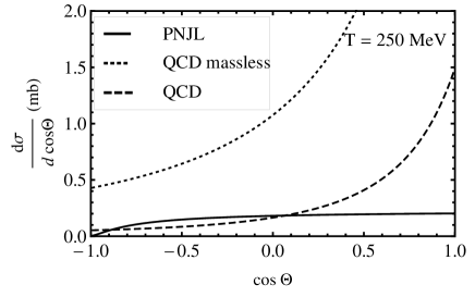
Figure 9: Comparison of the differential $ud\to ud$ cross section calculated in the pQCD model at $\sqrt{s}=$1 GeV for finite (dashed line) and vanishing (dotted line) masses. Our results for $T=$ 0.25 GeV are plotted by the solid line.

Such behavior is more transparent from simplified two-body pQCD calculations with $m=0$ used in the AMPT model [15]. In particular, for the gluon elastic scattering (which differs by the Casimir factor from the $qq$ scattering) one has

$$\frac{d\sigma_{gg}}{dt}=\frac{9\pi\alpha^{2}_{s}}{2s^{2}}(3-\frac{ut}{s^{2}}-\frac{us}{t^{2}}-\frac{st}{u^{2}})\simeq\frac{9\pi\alpha^{2}_{s}}{2}(\frac{1}{t^{2}}+\frac{1}{u^{2}})\simeq\frac{9\pi\alpha^{2}_{s}}{2t^{2}},$$ (44)

with the strong coupling constant $\alpha_{s}$. Equation (44) is obtained in the leading-order QCD by keeping only the leading divergent terms for identical particles, which allows one to limit oneself to the angle range $0\leq\Theta\leq\pi/2$ (the last equality in (44)). The cross section really diverges at the scattering angle $\Theta=$0. The singularity in this cross section can be regularized by introducing the Debye screening mass $M_{D}$ leading to

$$\frac{d\sigma_{gg}}{dt}=\frac{9\pi\alpha^{2}_{s}}{2(t-M_{D}^{2})^{2}}$$ (45)

and, respectively, for the total cross section at relativistic energies

$$\sigma_{gg}\simeq\frac{9\pi\alpha^{2}_{s}}{2M_{D}^{2}}\frac{1}{1+M_{D}^{2}/s}\approx\frac{9\pi\alpha^{2}_{s}}{2M_{D}^{2}}~{},$$ (46)

if $s\gg M^{2}_{D}$ [15]. Note that in this approximation the pQCD gives an energy-independent cross section (46) in disagreement with the NJL-like chiral model discussed. Taking $M_{D}=$3 fm^-1 we get $\sigma_{el}=$3 mb. In the real AMPT calculations $M_{D}$ is a parameter and this cross section changes from 3 to 10 mb in different model versions [15].

Quark-hadron elastic cross-section

The integral cross section for the in-medium elastic scattering of quarks on pions is presented in Fig. 10. For the

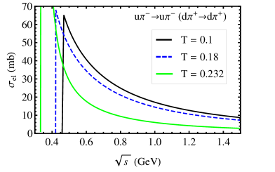
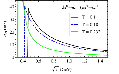
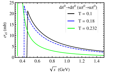
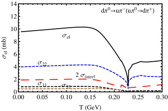
Figure 10: Energy dependence of the total scattering cross sections for the processes $qH\rightarrow qH$ corresponding to the different reactions and the temperature dependence of different components (see the text) of the $d\pi^{0}\to u\pi^{-}$ scattering cross section at $\sqrt{s}=$1 GeV (right-bottom panel).

considered reactions $u\pi^{-},d\pi^{+},u\pi^{0}$ and their charge conjugated ones the cross sections behave very similarly: $\sigma_{el}$ is maximal just at the threshold $s_{thr}=(m+m_{\pi}(T))^{2}$ reaching here values of 60-80 mb and then monotonically falls down rather quickly with the slightly different slopes for different reactions. At the Mott temperature and for all energies the $qH$ elastic cross section exhibits a huge maximum as large as several hundred of mb (to be cut in Fig.  10). Generally, the magnitude of the quark-pion cross sections is higher than the quark-quark one and comparable with free hadron-hadron cross sections. In the case of the $u\pi^{-}$ reaction, the cross section fall-off is the slowest, and the quark-pion scattering turns out to be several times higher than that for quark-quark in the energy range $\approx$(0.7-1.5) GeV.

As is seen from Fig. 10 (right-bottom panel), $\sigma_{el}(T)$ is a weakly changing function up to $T\sim$ 0.18 GeV and then has a kick at the Mott temperature. This cross section is the sum of different terms corresponding to the squared amplitudes: $\sigma_{11}$ (see Eq. (33)), $\sigma_{22}$ (Eq. (36)), $\sigma_{33}$ (Eq. (38)) and summary interference term $\sigma_{interf}$ (Eqs. (34)+(35)+(37)). The dominant $u$-channel gives $\sigma_{22}\sim 0.5\ \sigma_{el}$. In contrast, the cross section of the $t$-channel is very small, $\sigma_{33}\simeq$0.5 mb. The rest of $\sigma_{el}$ is shared almost equally between the sum of all interference terms $\sigma_{interf}$ (note the scale in figure) and the $s-$channel $\sigma_{11}$ elastic cross section.

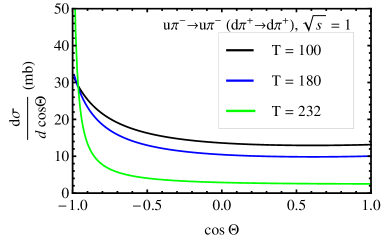
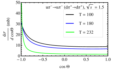
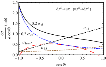
Figure 11: Angular distributions of the $u\pi^{-}\rightarrow u\pi^{-}$ scattering for all reactions at various temperatures and energies and the contributions of different channels of the $d\pi^{0}\to u\pi^{-}$ reaction to $d\sigma_{el}/dcos\Theta$ for $\sqrt{s}=$1 GeV and $T=$ 0.1 GeV (right-bottom panel). Notation of components is the same as in Fig. 10.

In Fig. 11, some examples of the angular distribution are given for the quark-pion scattering. At the energy $\sqrt{s}\stackrel{{\scriptstyle\scriptstyle<}}{{\phantom{}{}_{\sim}}}$ 0.5 GeV, independently of T, the angular distributions are isotropic with high accuracy, besides in the vicinity of $T_{Mott}$. At higher energy and moderate temperatures $T<T_{Mott}$ the differential distributions are almost isotropic with small anisotropy growing at the backward scattering angles. This backward bounce is more prominent for lower energies. The presented angular distributions are really the contributions of diagrams of three types (see Fig. 5). As is shown in the right-bottom panel of Fig. 11 and in accordance with the above discussion, $\sigma_{22}$ is dominant and completely defines the backward scattering (note the scale factor 0.2 in the figure). The $\sigma_{11}(\Theta)$ and $\sigma_{33}(\Theta)$ angular distributions are forward peaked but the asymmetry is much more pronounced in the $s$-channel. The sum of interference terms results in the distribution with a broad maximum at $cos\Theta\sim$0.

The presented results are the same for the $u\pi^{-}\to u\pi^{-}$ and $d\pi^{+}\to d\pi^{+}$ reactions because their flavor factors are the same (see Table II). For other channels of the quark-pion scattering, the shape of angular distributions is similar to that for $u\pi^{-}\to u\pi^{-}$ but the magnitude is lower in accordance with the flavor factors in Table II. Since a pion consists of a quark-antiquark pair, the substitution $u\to d$ for quarks does not change the calculated scattering cross sections results in Fig. 10 and angular distributions in the $s$- and $u$-channels shown in Fig. 11 are exchanged.

6 Concluding remarks

In-medium elastic scattering of quarks is evaluated by treating quarks in terms of the two-flavor PNJL model accounting for their scalar and pseudoscalar interactions and using the large $N_{c}$ approximation. The model parameters are in agreement with low-energy static mesonic properties and lattice QCD results for gluons. General trends of the energy and temperature dependence of $\sigma_{el}$ and $\d\sigma_{el}/dcos\Theta$ are investigated in a large range of $\sqrt{s}$ and $T$ at both below and above the Mott temperature. Essential influence of the flavor of interacting quarks on the scattering results is noted. The comparison with the earlier works shows that the $SU_{f}(2)$ PNJL results agree with those of the NJL model for the same $SU_{f}(2)$ symmetry (at $T>T_{Mott}$) but noticeably below in the case of three flavors. This difference is due to a larger number of contributing intermediate states for the quark scattering in the case of $SU_{f}(3)$ symmetry.

The above PNJL results are presented for the vanishing chemical potential. However, $\mu$ enters not only into the Pauli exclusion factor but also into the polarization function $\Pi(k^{2})$ which makes masses and coupling constants to be $\mu$-dependent. To consider the quark-baryon case, an additional issue arises: one should treat properly the loop formed by the quark and the diquark that form the baryon. As demonstrated in  [41], taking into account the finite chemical potential results in some suppression of the scattering cross sections at large $\mu$. The PNJL approach should also be generalized to the $SU_{f}(3)$ symmetry. This allows one to extend the set of reactions including strange quark and strange hadrons and to effect non-strange reactions due to increasing a number of possible intermediate states, as noted above. This work is in progress now.

The first predictions for the quark-pion scattering are given. The integral cross sections for this reaction are higher than those in the quark-quark case. The quark differential $cos\Theta$-distribution is practically constant with some enhancement in the backward direction at $\sqrt{s}\stackrel{{\scriptstyle\scriptstyle>}}{{\phantom{}{}_{\sim}}}$1 GeV. The developed technique and obtained results can be applied in the kinetic approach [15, 17, 22] to take into account the interaction between constituents of quark-gluon and hadronic phases. The derived formulae for the elastic quark-hadron scattering can be easily generalized to the expression for gamma and dielectron emission [42]. This new channel can definitely give rise to an observable effect and would confirm the existence of the quark-hadron interaction.

Another possible implementation of these results is a study of transport properties of the system. For example, the shear viscosity $\eta$ can be estimated in the so-called relaxation time approximation by using the average momentum loss $\bar{p}$, the quark densities $n_{i}$ and the mean life time as $\displaystyle\eta\sim\sum_{i}n_{i}\bar{p}_{i}/\lambda_{i}$, the mean life time being inversely proportional to the quark cross sections $\displaystyle\lambda^{-1}=\sum_{i}n_{i}\sigma_{qi}$ Ref. [43]. In the two-flavor NJL model, this shear viscosity was estimated in Ref. [34] for the chiral limit $m=0$. One should not expect a noticeable difference with our model treating a quark system with the finite quark masses in the $SU_{f}(2)$ PNJL model, especially at high temperature where the NJL model is more justified. However, for the mixed quark-hadron system considered in [15, 17, 22] the shear viscosity should be smaller, because the $qH$ elastic cross section is noticeably larger than the quark-quark one and particle density of quarks and pions is rather abounded in the mixed phase. Certainly, this problem deserves a more elaborated study, for example, by the method developed in Ref. [44] .

Acknowledgments
We would like to thank H. Berrehrah, R. Marty and V. Priezzhev for fruitful discussions and constructive remarks. We are grateful to E. Bratkovskaya, W. Cassing and O. Linnyk for their continuous interest in this work. This work was supported in part (Yu. K.) by RFFI grants 13-01-00060, 12-01-00396.

References

- [1] Y. Nambu and G. Jona-Lasinio, Phys.Rev. 122 (1961) 345 ; Phys. Rev. 124 (1961) 246.
- [2] A.M. Polyakov, Phys. Lett. B 72 (1978) 477.
- [3] K. Fukushima, Phys. Lett. B 591 (2004) 277; arXiv:1008.4322.
- [4] Y. Hatta and K. Fukushima, arXiv:hep-ph/0311267.
- [5] C. Ratti, M.A. Thaler and W. Weise, Phys. Rev. D 73 (2006) 014019; arXiv:nucl-th/0604025.
- [6] C. Ratti, S. Roessner, M. A. Thaler and W. Weise, Eur. Phys. J. C 49 (2007) 213.
- [7] P. Costa, M.C. Ruivo, C. A. de Sousa and H. Hansen, Symmetry 2 (2010) 1338.
- [8] S. Mukherjee, M.G. Mustafa and R. Ray, Phys. Rev. D 75 (2007) 094015.
- [9] Y. Sakai, T. Sasaki, H. Kouno and M. Yahiro, arXiv:1010.5865.
- [10] H. Abuki, M. Ciminale, R. Gatto, N. D. Ippolito, G. Nardulli and M. Ruggieri, Phys. Rev. D 78 (2008) 014002 (2008).
- [11] P.N. Meisingera, M.C. Ogilviea and T.R. Millerb, Phys. Lett. B585 (2004) 149.
- [12] M. Ruggieri, P. Alba, P. Castorina, S. Plumari, C. Ratti and V. Greco, Phys. Rev. D 86 (2012) 054007.
- [13] C. Sasaki and K. Redlich, Phys. Rev. D 86 (2012) 014007.
- [14] L. Oliva, P. Castorina, V. Greco and M. Ruggieri, arXiv:1309.6541.
- [15] Z.W. Lin, C.M. Ko, B.A. Li, B. Zhang and S. Pal, Phys. Rev. C72 (2005) 064901.
- [16] W. Cassing, Eur. Phys. J. ST 168 (2009) 3.
- [17] W. Cassing and E.L. Bratkovskaya, Nucl. Phys. A 831 (2009) 215.
- [18] E.L. Bratkovskaya, W. Cassing, V.P. Konchakovski and O. Linnyk, Nucl. Phys. A 856 (2011) 162.
- [19] Z. Xu and C. Greiner, Phys. Rev. C 71 (2005) 064901; J. Uphoff, O. Fochler, Z. Xu, and C. Greiner, Phys. Rev. C 82 (2010) 044906.
- [20] G. Ferini, M. Colonna, M. Di Toro and V. Greco, Phys. Lett. B 670 (2009) 325.
- [21] F. Scardina, M. Colonna, S. Plumari and V. Greco, arXiv:1202.2262.
- [22] R. Marty and J. Aichelin, Phys. Rev. C 87 (2013) 034912.
- [23] A.A. Shanenko, E.P. Yukalova and V.I. Yukalov, Phys. Atom. Nucl. 56 (1993) 372 , Yad. Fiz. 56(3) (1993) 151.
- [24] M. Asakawa and K. Yazaki Nucl. Phys, A 504 (1989) 668.
- [25] K. Fukushima, Phys. Rev. D 77 (2008) 114028, Erratum-ibid D 78 (2008) 039902.
- [26] S. Carignano, D. Nickel and M. Buballa, Phys. Rev. D 82 (2010) 054009.
- [27] N. Bratovich, T. Hatsuda and W. Weise, arXiv:1204.3788.
- [28] R.D. Pisarski, Phys. Rev. D 62 (2000) 111501.
- [29] H. Hansen, W.M. Flberico, A. Beraudo, A. Molinari, M. Nardi and C. Ratti, Phys. Rev. D 75 (2007) 065004.
- [30] S. Rössner, C. Ratti and W. Weise, Phys. Rev. D 75 (2007) 034007.
- [31] S.P. Klevansky, Rev. Mod. Phys. 64 (1992) 649.
- [32] A.V. Friesen, Yu.L. Kalinovsky and V.D. Toneev, Phys. Part. Nucl. Lett. 9 (2012) 8.
- [33] P. Rehberg, S.P. Klevansky and J. Hüfner, Nucl. Phys. A 608 (1996) 356.
- [34] P. Zhuang, J. Hüfner, S.P. Klevansky and L. Neise, Phys. Rev. D 51 (1995) 3728.
- [35] P. Rehberg, S.P. Klevansky and J. Hüfner, Phys. Rev. C 53 (1996) 410.
- [36] A.V. Friesen, Yu.L. Kalinovsky and V.D. Toneev, Int. Jour. of Modern Phys. A 27 (2012) 12500133.
- [37] P. Rehberg, Yu.L. Kalinovsky and D. Blaschke, Nucl.Phys. A 622 (1997) 478.
- [38] E. Quack, P. Zhuang, Y. Kalinovsky, S.P. Klevansky and J. Hüfner, Phys. Lett, B 348 (1995) 1.
- [39] A.E. Dorokhov, M.K. Volkov, J. Hüfner, S.P. Klevansky and P. Rehberg, Z. Phys. C 75 (1997) 127.
- [40] K. Geiger, Phys. Rep. 258 (1995) 237.
- [41] E. Blanquier, J. Phys. G: Nucl. Phys. 39 (2012) 10503.
- [42] O. Linnyk, W. Cassing, J. Manninen, E.L. Bratkovskaya and C.M. Ko, Phys.Rev. C 85 (2012) 024910.
- [43] A.S. Khvorostukhin, V.D. Toneev and D.N. Voskresensky, Nucl. Phys. A 845 (2010) 106.
- [44] V. Ozvenchuk, O. Linnyk, M.I. Gorenstein, E.L. Bratkovskaya and W. Cassing, Phys. Rev. C 87 (2013) 024901.