Negativity as a counter of entangled dimensions

Abstract

Among all entanglement measures negativity arguably is the best known and most popular tool to quantify bipartite quantum correlations. It is easily computed for arbitrary states of a composite system and can therefore be applied to discuss entanglement in an ample variety of situations. However, its direct physical meaning has not been pointed out yet. We show that the negativity can be viewed as an estimator of how many degrees of freedom of two subsystems are entangled. As it is possible to give lower bounds for the negativity even in a device-independent setting, it is the appropriate quantity to certify quantumness of both parties in a bipartite system and to determine the minimum number of dimensions that contribute to the quantum correlations.

Introduction. – The dimension, that is, the number of independent degrees of freedom is a particularly important system parameter. It is relevant, for example, for the security of cryptography schemes and for the significance of Bell inequality violation Acin2006 ; Brunner2008 . In general, in information processing (both classical and quantum) the dimensionality may be regarded as a resource and is therefore crucial for system performance.

The device-independent characterization of physical systems Acin2006 ; Brunner2008 ; Gallego2010 ; Bancal2011 ; Pal2011 ; Bancal2012 ; Acin2012 ; Cabello2012 ; Moroder2013 without a priori restrictions regarding the underlying structure of mathematical models is fundamental for our understanding of Nature. The goal is to obtain the desired physical information based only on the statistics from certain measurement outcomes (’prepare and measurement scenario’, Ref. Gallego2010 ) without reference to internal properties or mechanisms of a device. In recent years numerous schemes for device-independent dimension testing and other system properties have been proposed. There are methods that detect the minimum number of classical or quantum degrees of freedom for a single system Gallego2010 ; Acin2012 ; Cabello2012 . The dimensionality may be inferred also from Bell-inequality violation Acin2006 ; Brunner2008 . On the other hand, there are device-independent methods for multipartite entanglement detection Bancal2011 ; Pal2011 ; Bancal2012 ; Moroder2013 . In our work we propose direct counting of entangled dimensions based on a well-known entanglement measure for bipartite systems, the negativity, thereby elucidating the physical meaning of the latter. The method can be made device independent by invoking techniques from Refs. Bancal2012 ; Moroder2013 . With our result we cannot draw any conclusion regarding the classical dimensions of the two local systems. However, since entanglement is possible only between quantum degrees of freedom we directly obtain the minimum number of quantum levels for both parties which then are certified to be quantum without further assumption.

To demonstrate this we first study a nontrivial family of mixed states that can be defined for any $d\times d$-dimensional bipartite system, the axisymmetric states. Their negativity provides a clear illustration for the central statement of our article. It is then easy to show that this statement holds for arbitrary states as well. Finally we establish the link to the device-independent description that concludes our construction of a device-independent bound on the number of entangled dimensions for two-party systems.

Negativity. – The negativity was first used by Zyczkowski et al. Zyczkowski1998 and subsequently introduced as an entanglement measure by Vidal and Werner VidalWerner2002 . Consider the state $\rho$ of a bipartite system with finite-dimensional Hilbert space $\mathcal{H}_{A}\otimes\mathcal{H}_{B}$. The negativity is defined as

$$\mathcal{N}(\rho)\ =\ \frac{1}{2}\left(||\rho^{T_{A}}||_{1}-1\right)$$ (1)

where $\rho^{T_{A}}$ denotes the partial transpose with respect to party $A$ and $||M||_{1}\equiv\operatorname{tr}\sqrt{M^{\dagger}M}$ is the trace norm of the matrix $M$. We slightly modify this definition by introducing the quantity

$$\mathcal{N}_{\text{dim}}(\rho)\ =\ 2\ \mathcal{N(\rho)}+1\ \equiv\ ||\rho^{T_{A}}||_{1}\ \ .$$ (2)

As our discussion proceeds it will turn out that the least integer greater than or equal to $\mathcal{N}_{\text{dim}}$ is a lower bound to the number of entangled dimensions between the parties $A$ and $B$.

Axisymmetric states. – In studies of entanglement properties it is often useful to define families of states with a certain symmetry Vollbrecht2001 , such as the Werner states Werner1989 and the isotropic states Horodecki1999 . Here we introduce the axisymmetric states $\rho^{\text{axi}}$ for two qudits which are all the states obeying the same symmetries as the maximally entangled state in $d$ dimensions

$$|\Psi_{d}\rangle\ =\ \frac{1}{\sqrt{d}}\left(|11\rangle+|22\rangle+\ldots+|dd\rangle\right)\ \ ,$$ (3)

that is

• exchange of the two qudits,

• simultaneous permutations of the basis states for both qudits e.g., $|0\rangle_{A}\leftrightarrow|1\rangle_{A}$ and $|0\rangle_{B}\leftrightarrow|1\rangle_{B}$,

• coupled phase rotations

  $$U(\varphi_{1},\ldots,\varphi_{d-1})=\mathrm{e}^{\mathrm{i}\sum_{j}\varphi_{j}\mathfrak{g}_{j}}\otimes\mathrm{e}^{-\mathrm{i}\sum_{k}\varphi_{k}\mathfrak{g}_{k}}$$

  where $\mathfrak{g}_{j}$ ($j=1,\ldots,d-1$) are the diagonal generators of the group SU($d$).

Apart from the maximally entangled state Eq. (3) this family contains only (mostly full-rank) mixed states. For any $d\geqq 2$ these states are given by two real parameters $x$ and $y$ that describe the position of the state in a plane triangle (in close analogy to the Greenberger-Horne-Zeilinger symmetric states Eltschka2012 ), see Fig. 1. In order to determine the lengths of the triangle sides we choose the Euclidean metric of the triangle to coincide with the Hilbert-Schmidt metric of the density matrices. This enables us to deduce various physical facts from Fig. 1 merely by means of geometric intuition.

Axisymmetric states for $d\times d$ systems can be represented as $d^{2}\times d^{2}$ matrices with diagonal elements

$$\rho^{\text{axi}}_{jj,jj}\ =\ \frac{1}{d^{2}}+a\ ,\ \ \ \rho^{\text{axi}}_{jk,jk}\ =\ \frac{1}{d^{2}}-\frac{a}{d-1}\ \ (j\neq k)$$

($j,k=1,\ldots,d$) and off-diagonal entries

$$\rho^{\text{axi}}_{jj,kk}\ =\ b\ \ (j\neq k)\ \ ,$$

all other off-diagonal elements vanish. The ranges for the matrix elements are

$$-\frac{1}{d^{2}}\ \leqq\ a\ \leqq\ \frac{d-1}{d^{2}}$$ (4)

$$-\frac{1}{d-1}\left(\frac{1}{d^{2}}+a\right)\ \leqq\ b\ \leqq\ \left(\frac{1}{d^{2}}+a\right)\ \ .$$ (5)

From Eqs. (4), (7) we recognize the triangular shape of the set of axisymmetric states. With this choice of parametrization the fully mixed state $\frac{1}{d^{2}}{\rm 1\kern-2.20001ptl}_{d^{2}}$ is located at the origin.

Now we choose the scale of $a\equiv\alpha y$ and $b\equiv\beta x$ such that the Euclidean metric for $x$ and $y$ with the Hilbert-Schmidt metric in the space of density matrices. We define the Hilbert-Schmidt scalar product of two matrices $M_{1}$ and $M_{2}$ as $\langle M_{1},M_{2}\rangle_{\text{HS}}\equiv\operatorname{tr}\left(M_{1}^{\dagger}M_{2}\right)$. With this we find $\alpha=\frac{\sqrt{d-1}}{d}$ and $\beta=\sqrt{d(d-1)}^{-1}$ so that

$$-\frac{1}{d\sqrt{d-1}}\ \leqq\ y\ \leqq\ \frac{\sqrt{d-1}}{d}$$ (6)

$$-\frac{1}{\sqrt{d(d-1)}}\ \leqq\ x\ \leqq\ \sqrt{\frac{d-1}{d}}\ \ .$$ (7)

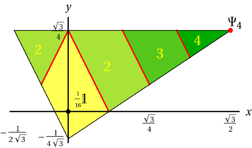
Figure 1: The convex set of $d\times d$ axisymmetric states $\rho^{\text{axi}}$, here for $d=4$. The family is characterized by two real parameters. While $x$ is proportional to the off-diagonal element, $y$ describes the asymmetry between the two types of diagonal elements (see Section Methods). The upper right corner corresponds to the maximally entangled state $|\Psi_{d}\rangle$ (the only pure state), the completely mixed state $\frac{1}{d^{2}}{\rm 1\kern-2.20001ptl}_{d^{2}}$ resides at the origin.
The states with local dimension $d$ have $d$ SLOCC classes corresponding to their Schmidt number $k$ (indicated by the yellow numbers in the regions). The states with Schmidt number $\leqq k$ form the convex sets $S_{k}$ and build a hierarchy $S_{1}\subset S_{2}\subset\ldots\subset S_{d}$. Note that Schmidt number $k=1$ corresponds to separable states which are considered classical.

Entanglement of axisymmetric states. – Remarkably, many entanglement properties of axisymmetric states can be determined exactly. The entanglement class of a bipartite state with respect to stochastic local operations and classical communication (SLOCC) is given by its Schmidt number, the minimal required Schmidt rank for any pure-state decomposition of the state. By using the optimal Schmidt number witnesses Lewenstein2001

$$\mathcal{W}\ =\ \frac{k-1}{d}\ {\rm 1\kern-2.20001ptl}_{d^{2}}-|\Psi_{d}\rangle\!\langle\Psi_{d}|$$

($2\leqq k\leqq d)$ we find for each state $\rho^{\text{axi}}(x,y)$ the corresponding Schmidt number, cf. Fig. 1. Notably, the borders between the SLOCC classes for $x\geqq 0$ are straight lines parallel to the lower left side of the triangle. This is no surprise since those lines correspond to states of constant overlap with the maximally entangled state $|\Psi_{d}\rangle$. Moreover, we easily identify the compact convex sets $S_{k}$ of states with Schmidt number at most equal to $k$ Lewenstein2001 .

In the next step, we calculate the negativity for axisymmetric states. To this end we consider the eigenvalue problem for the partial transpose of $\rho^{\text{axi}}$. It results in $\frac{d(d-1)}{2}$ identical eigenvalue problems for $2\times 2$ matrices

$$\begin{pmatrix}\frac{1}{d^{2}}-\frac{a}{d-1}&b\\ b&\frac{1}{d^{2}}-\frac{a}{d-1}\end{pmatrix}$$

which have the eigenvalues

$$\lambda_{\pm}\ =\ \frac{1}{d^{2}}-\frac{a}{d-1}\ \pm\ |b|\ \ .$$

Adding the absolute negative eigenvalues and rewriting $a$ and $b$ in terms of $x$ and $y$ leads to

$$\mathcal{N}=\max\left\{0,\frac{1}{2}\left(\sqrt{d(d-1)}|x|+\sqrt{d-1}y-\frac{d-1}{d}\right)\right\}\ .$$ (8)

From this we find the exact $\mathcal{N}_{\text{dim}}$ for the entangled axisymmetric states

$$\mathcal{N}_{\text{dim}}(\rho^{\text{axi}}(x,y))\ =\ \sqrt{d(d-1)}|x|+\sqrt{d-1}y+\frac{1}{d}$$ (9)

which is noteworthy in several respects. First, the negativity is a linear function of $|x|$ and $y$ (see Fig. 2). A state has nonvanishing negativity if and only if it is not separable. Consequently, there are no entangled axisymmetric states with positive partial transpose. Further, and most importantly, the borders between SLOCC classes correspond to isolines for integer values of the negativity. With the ceiling function $\lceil x\rceil$, the smallest integer greater than or equal to $x$, we see that for axisymmetric states $\rho^{\text{axi}}(x,y)$

$$\text{SLOCC\ class}\ k\ \ =\ \lceil\mathcal{N}_{\text{dim}}(x,y)\rceil\ \ .$$ (10)

However, the SLOCC class, that is, the minimum required Schmidt rank of the pure states in the decomposition of $\rho^{\text{axi}}$ counts the number of degrees of freedom in which subsystems $A$ and $B$ are entangled. In consequence our result implies that for axisymmetric states the modified negativity $\mathcal{N}_{\text{dim}}$ is a precise counter of entangled dimensions.

Dimension estimator for arbitrary states. – Naturally the question is imposed to which extend this statement holds for all bipartite states. Due to the existence of entangled states with positive partial transpose Horodecki1998 it is clear that the negativity cannot be a precise counter of entangled dimensions for arbitrary states. In the following we prove that, while not being an exact counter, the modified negativity $\mathcal{N}_{\text{dim}}$ is always a lower bound to the Schmidt number.

To this end, we explicitly show again how to calculate the negativity for pure entangled states of Schmidt rank $k$. Any such state is locally equivalent to $|\Psi_{k}\rangle$, the maximally entangled state of Schmidt rank $k$. Considering the partial transpose of $|\Psi_{k}\rangle\!\langle\Psi_{k}|$

$$|\Psi_{k}\rangle\!\langle\Psi_{k}|=\frac{1}{k}\sum_{\alpha\beta}|\alpha\alpha\rangle\!\langle\beta\beta|\ \ \stackrel{{\scriptstyle T_{A}}}{{\longrightarrow}}\ \ \frac{1}{k}\sum_{\alpha\beta}|\beta\alpha\rangle\!\langle\alpha\beta|$$

it is evident that $\mathcal{N}_{\text{dim}}(\Psi_{k})=2\frac{1}{k}\frac{k(k-1)}{2}+1=k$. Now, since according to Ref. VidalWerner2002 the negativity is a convex function of the state $\rho$ we find for an arbitrary state of Schmidt number $k$

$$\mathcal{N}_{\text{dim}}(\rho)\ \leqq\ \sum_{j}p_{j}\mathcal{N}_{\text{dim}}(\psi_{j})\ \leqq\ \sum_{j}p_{j}k\ =\ k$$ (11)

for $\rho=\sum_{j}p_{j}|\psi_{j}\rangle\!\langle\psi_{j}|$ as in that case $\mathcal{N}_{\text{dim}}(\psi_{j})\leqq k$. We mention that these estimates are valid for arbitrary bipartite systems with $d\times d^{\prime}$ dimensions, both for $d=d^{\prime}$ and for $d\neq d^{\prime}$. This is because the Schmidt rank of a pure $d\times d^{\prime}$ state cannot exceed the smaller of the two local dimensions. This concludes the proof that the modified negativity $\mathcal{N}_{\text{dim}}$ is an estimator for the number of entangled dimensions of arbitrary two-party states. $\Box$

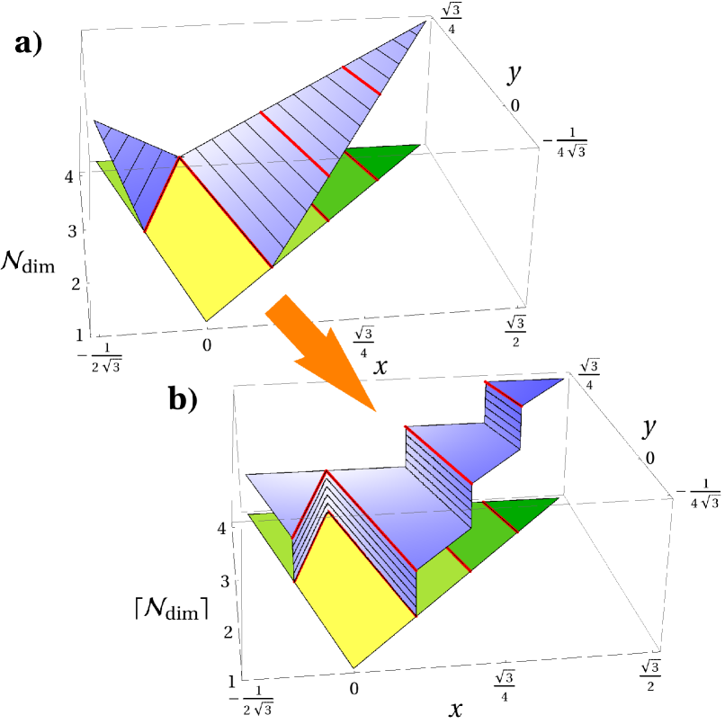
Figure 2: Exact modified negativity $\mathcal{N}_{\text{dim}}$ for $d\times d$ axisymmetric states $\rho^{\text{axi}}$, again for $d=4$.
a) The blue surface displays $\mathcal{N}_{\text{dim}}(x,y)$. It depends linearly on $|x|$ and $y$. Note that the borders between SLOCC classes (red lines in the $x,y$ plane) are projections of integer-value isolines of the modified negativity.
b) The ceiling function $\lceil\mathcal{N}_{\text{dim}}(x,y)\rceil$ (blue surface) counts the Schmidt number of $\rho^{\text{axi}}(x,y)$.

Device-independent dimension estimate. – It remains to discuss that a lower bound on the entangled dimensions via the negativity, or $\mathcal{N}_{\text{dim}}$, can be obtained in a device-independent setting. This technique has rencently been worked out by Moroder et al. Moroder2013 and we sketch only the main idea here. A device-independent scenario implies that a number of generalized measurements are carried out on the subsystems $A$ and $B$. While the detailed actions $A_{i}$, $B_{j}$ of the measurement devices on the true state $\rho_{AB}$ are unknown to the observers, the outcomes for each party labeled by $i$ and $j$, are mutually exclusive. One also defines $A_{0}={\rm 1\kern-2.20001ptl}_{A}$ and $B_{0}={\rm 1\kern-2.20001ptl}_{B}$. The observers ’see’ $\rho_{AB}$ only via their preparation-measurement setup, and (partially) determine the Hermitian matrix

$$\chi_{ij,kl}[\rho_{AB}]=\operatorname{tr}\left[\rho_{AB}\left(A_{k}^{\dagger}A_{i}\otimes B_{l}^{\dagger}B_{j}\right)\right]$$ (12)

with orthonormal bases $\{|i\rangle_{\tilde{A}}\}$, $\{|j\rangle_{\tilde{B}}\}$ in the outcome spaces $\tilde{A}$ and $\tilde{B}$. This matrix depends linearly on $\rho_{AB}$ and is positive whenever the true state $\rho_{AB}$ is positive. Correspondingly, whenever $\rho_{AB}^{T_{A}}$ is positive, $\chi^{T_{A}}$ is positive, too.

The possibility to estimate the negativity relies on its variational expression VidalWerner2002 : $\mathcal{N}(\rho_{AB})=\min\{\operatorname{tr}\sigma:\mbox{$\sigma^{T_{A}}\geqq 0$},(\rho_{AB}-\sigma)^{T_{A}}\geqq 0\}$. The properties of $\chi$ mentioned above mean that the conditions for minimization hold also for $\chi[\rho_{AB}]$ and $\chi[\sigma]$. Moreover, the optimized quantity $\operatorname{tr}\sigma$ equals $\chi_{0000}[\sigma]$. Therefore, minimising $\chi_{0000}[\sigma]$ over all matrices $\chi$ consistent with the measurement outcomes(and the condition $\operatorname{tr}\rho_{AB}=1$) will give a lower bound for the negativity $\mathcal{N}(\rho_{AB})$.

Evidently, our findings are useful to characterize a test system with unknown quantum dimension. By entangling it with an auxiliary system of known dimension and measuring the negativity a lower bound to the number of quantum levels in the test system can be found.

We conclude by mentioning that the results regarding the negativity hold also for the convex-roof extended negativity Lee2003 because it is the largest convex function that coincides with the negativity on pure states Uhlmann2010 . However, while improving the estimate in Eq. (11) the negativity would forfeit its most important asset, namely that it can be calculated easily.

Acknowledgements – . This work was funded by the German Research Foundation within SPP 1386 (C.E.), and by Basque Government grant IT-472 (J.S.). The authors thank O. Gühne and Z. Zimboras for helpful remarks and J. Fabian and K. Richter for their support.

References

- (1) A. Acín, N. Gisin, and Ll. Masanes, Phys. Rev. Lett. 97, 120405 (2006).
- (2) N. Brunner, S. Pironio, A. Acin, N. Gisin, A. Méthot, and V. Scarani, Phys. Rev. Lett. 100, 210503 (2008).
- (3) R. Gallego, N. Brunner, C. Hadley, and A. Acín, Phys. Rev. Lett. 105, 230501 (2010).
- (4) J.-D. Bancal, N. Gisin, Y.-C. Liang, and S. Pironio, Phys. Rev. Lett. 106, 250404 (2011).
- (5) K.F. Pál, and T. Vértesi, Phys. Rev. A 83, 062123 (2011).
- (6) J.-D. Bancal, C. Branciard, N. Brunner, N. Gisin, and Y.-C. Liang, J. Phys. A: Math. Theor. 45, 125301 (2012).
- (7) M. Hendrych, R. Gallego, M. Mičuda, N. Brunner, A. Acín, and J.-P. Torres, Nat. Phys. 8, 588 (2012).
- (8) J. Ahrens, P. Badziag, A. Cabello, and M. Bourennane, Nat. Phys. 8, 592 (2012).
- (9) T. Moroder, J.-D. Bancal, Y.-C. Liang, M. Hofmann, and O. Gühne, e-print arXiv:1302.1336 (2013).
- (10) K.G.H. Vollbrecht and R.F. Werner, Phys. Rev. A 64, 062307 (2001).
- (11) R.F. Werner, Phys. Rev. A 40, 4277 (1989).
- (12) M. Horodecki, and P. Horodecki, Phys. Rev. A 59, 4206 (1999).
- (13) K. Zyczkowski, P. Horodecki, A. Sanpera, and M. Lewenstein, Phys. Rev. A 58, 883 (1998).
- (14) G. Vidal, and R.F. Werner, Phys. Rev. A 65, 032314 (2002).
- (15) C. Eltschka, and J. Siewert, Phys. Rev. Lett. 108, 020502 (2012).
- (16) A. Sanpera, D. Bruß, and M. Lewenstein, Phys. Rev. A 63, 050301 (2001).
- (17) M. Horodecki, P. Horodecki, and R. Horodecki, Phys. Rev. Lett. 80, 5239 (1998).
- (18) S. Lee, D.-P. Chi, S.-D. Oh, and J. Kim, Phys. Rev. A 68, 062304 (2003).
- (19) A. Uhlmann, Entropy 12, 1799 (2010).