Line defects in Three dimensional Symmetry Protected Topological Phases

Abstract

A 3d symmetry protected topological phase, by definition must have symmetry protected nontrivial boundary states, namely its 2d boundary must be either gapless or degenerate. In this work we demonstrate that once we couple a 3d SPT phase to a lattice dynamical $Z_{2}$ gauge field, in many cases the $Z_{2}$ vison loop excitation (line defect) can be viewed as a “1d boundary” of the 3d SPT phase, and this line defect is guaranteed to have gapless or degenerate spectrum, which is also protected by the symmetry of the SPT phase.

In the last few years, motivated by the discovery of free fermion topological insulators protected by time-reversal symmetry Kane and Mele (2005a, b); Bernevig et al. (2006); Moore and Balents (2007); Fu et al. (2007); Roy (2009), a new class of quantum disordered states, the so called symmetry protected topological (SPT) phases was proposed Chen et al. (2011, 2012). Unlike intrinsic topological phases such as fractional quantum Hall states, a SPT phase is only nontrivial when the system has certain symmetry $G$. A $d-$dimensional SPT phase must have a fully gapped and nondegenerate spectrum in the bulk, and also a gapless or degenerate spectrum on its $d-1$ dimensional boundary, when and only when the Hamiltonian of the system (both in the bulk and the boundary) has symmetry $G$. In the last two years, SPT phase has emerged as a new subfield of condensed matter theory, and it has attracted a lot of attentions and efforts Chen et al. (2011, 2012); Senthil and Levin (2013); Levin and Stern (2012); Liu and Wen (2013); Lu and Vishwanath (2012); Vishwanath and Senthil (2013); Xu (2013); Oon et al. (2012); Xu and Senthil (2013); Wang and Senthil (2013); Chen et al. (2013); Metlitski et al. (2013); Ye and Wen (2012, 2013).

Based on the definition of SPT phases, the 2d boundary of a 3d SPT phase must have nontrivial spectrum. But the properties of a 1d boundary (or 1d line defect) in a 3d SPT has not been studied yet. Line defects in ordinary topological insulators have been discussed before, and it was pointed out that these line defects do carry gapless modes localized along the defects Ran et al. (2009a, b). In this work we will study one type of line defects in strongly interacting 3d bosonic SPT phases, and we will conclude that in many cases, this line defect in a 3d SPT phase does lead to gapless or degenerate spectrum.

Since so far we do not have explicit lattice model for most of the SPT phases under study, our work will be based on the effective field theory of SPT phases. Trivial quantum disordered phases can be described as the disordered phase of either a Ginzburg-Landau field theory, or a semiclassical nonlinear sigma model (NLSM) defined with an order parameter. SPT phases have the same bulk spectrum and bulk phase diagram as a trivial system, so they can still be described by NLSMs, and their nontrivial boundary spectrum can be captured with a topological $\Theta-$term in the bulk Vishwanath and Senthil (2013); Xu (2013). It was demonstrated that the NLSM plus an appropriate topological $\Theta-$term not only leads to nontrivial boundary physics Xu and Ludwig (2011), it also gives us the correct ground state wave function of the SPT phase Xu and Senthil (2013). In this work we will focus on several 3d SPT phases that are described by the same effective field theory, which is a O(5) Nonlinear Sigma model with a $\Theta-$term at $\Theta=2\pi$:

$$S=\int d^{3}xd\tau\ \frac{1}{g}(\partial_{\mu}\vec{n})^{2}+\frac{i\Theta}{\Omega_{4}}\epsilon_{abcde}n^{a}\partial_{x}n^{b}\partial_{y}n^{c}\partial_{z}n^{d}\partial_{\tau}n^{e}.$$ (1)

Here $\vec{n}$ is a five-component order parameter with unit length. Although these SPT phases share the same effective field theory, the vector order parameter $\vec{n}$ transforms differently under symmetry in different SPT classes.

The order parameter $\vec{n}$ corresponds to certain operators on the lattice scales, such as spin and boson operators. As long as the symmetry of the SPT phase contains a $Z_{2}$ center, $i.e.$ a $Z_{2}$ subgroup that commutes with all the other group elements, we can always modify the Hamiltonian by coupling the lattice operators to a dynamical $Z_{2}$ gauge field on the lattice. Since the matter field $\vec{n}$ is disordered and gapped in the bulk of these SPT phases, the $Z_{2}$ gauge field can have a deconfined phase, which is the phase we will focus on in this paper. The deconfined phase of a $Z_{2}$ gauge field introduces line defect in the system, which is the vison loop of the $Z_{2}$ gauge field, $i.e.$ a $\pi-$flux loop in the system. We will argue that in many SPT phases described by Eq. 1, the vison loop has a nontrivial spectrum, namely it is either gapless or degenerate.

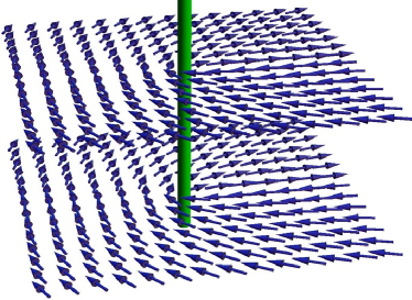
Figure 1: A vison loop in example 1 and 2 is bound with a half vortex line of $b\sim n^{1}+in^{2}$, which leads to a 1+1d O(3) NLSM with $\Theta=\pi$ along the vison loop.

Example 1: 3d SPT with $[U(1)\times U(1)]\rtimes Z_{2}^{T}$

Let us start with a simple example of 3d SPT phase with $[U(1)\times U(1)]\rtimes Z_{2}^{T}$ symmetry, where $Z_{2}^{T}$ is the time-reversal symmetry. This SPT phase is described by Eq. 1 where $n^{1}+in^{2}\sim b_{1}$ and $n^{3}+in^{4}\sim b_{2}$ are two independent boson fields, and $n^{5}=\phi$ is an Ising order parameter that changes sign under $Z_{2}^{T}$ Vishwanath and Senthil (2013):

$$Z_{2}^{T}:b_{1}\rightarrow b_{1},\ \ b_{2}\rightarrow b_{2},\ \ \phi\rightarrow-\phi.$$ (2)

Eq. 1 has an enlarged SO(5) symmetry, but we can turn on extra terms in Eq. 1 which reduce this symmetry down to physical symmetry $[U(1)\times U(1)]\rtimes Z_{2}^{T}$.

We will focus on the SPT phase, namely the phase where the five component order parameter $\vec{n}$ is completely disordered. We can couple $b_{1}$ to a $Z_{2}$ gauge field, and let us assume this $Z_{2}$ gauge field is deep in its deconfined phase, namely the vison loop excitations of this phase are gapped and dilute. Although we do not yet have an explicit lattice model for this 3d SPT, the lattice model of this SPT phase must only contain terms that are even powers of $b_{1}$ and $b_{1}^{\dagger}$ in order to keep the U(1) symmetry: $H_{0}=\sum_{i,j}-tb^{\dagger}_{1,i}b_{1,j}+\cdots$. Thus we can modify this Hamiltonian and couple $b_{1}$ to a $Z_{2}$ gauge field $\sigma^{z}_{ij}$ defined on the links of the lattice: $H_{g}=\sum_{i,j}-t\sigma^{z}_{ij}b^{\dagger}_{1,i}b_{1,j}+\cdots$

Now consider a long vison loop along $z$ axis. This vison loop is bound with a half-vortex line of $b_{1}$ (Fig. 1), and the vison loop is the core of the half-vortex line. Along the vison loop (core of half-vortex line), since $n^{1}$ and $n^{2}$ are zero, the effective Lagrangian along the vison loop only involves a three component unit vector $\vec{n}=(n^{3},n^{4},n^{5})\sim(\mathrm{Re}[b_{2}],\mathrm{Im}[b_{2}],\phi)$. The effective action along the vison loop reads

$$\mathcal{S}_{v} = \int dzd\tau\frac{1}{g^{\prime}}(\partial_{\mu}\vec{n})^{2}+\frac{i\Theta_{1d}}{8\pi}\epsilon_{\mu\nu}\epsilon_{abc}n^{a}\partial_{\mu}n^{b}\partial_{\nu}n^{c},$$ (3)

$$\Theta_{1d} = \oint d\vec{l}\ \epsilon_{ef}n^{e}\partial_{l}n^{f}=\pi,\ \ \ e,f=1,2.$$ (5)

where $l$ is the line coordinate along a large closed circle around the vison loop.

In Eq. 5, $\Theta_{1d}=\pi$ is protected by time-reversal symmetry. Under $Z_{2}^{T}$, since a vortex of $b_{1}$ transforms into an anti-vortex of $b_{1}$, the derived 1d $\Theta-$term changes its sign: $\Theta_{1d}\rightarrow-\Theta_{1d}$, hence Eq. 5 is only time-reversal invariant at points $\Theta_{1d}=\pi k$ with integer $k$. If we ignore the physical interpretation of the field $\vec{n}$, this 1+1d NLSM at $\Theta_{1d}=\pi$ (Eq. 5) can be used to describe the antiferromagnetic spin-1/2 chain, and based on the Lieb-Schultz-Mattis (LSM) theorem this 1+1d system must be either gapless or degenerate Lieb et al. (1961). When it is gapless, the vison loop is described by a 1+1d conformal field theory; degenerate ground state can be induced by spontaneous time-reversal symmetry breaking along the vison loop.

Notice that the vison loop is invariant under time-reversal transformation, because in one plaquette $\pi-$flux and $-\pi-$flux are equivalent. However, flux lines of other discrete gauge fields are not necessarily time-reversal invariant, thus if we couple the same SPT phase to other discrete gauge fields, the line defects may be fully gapped without degeneracy.

Example 2: 3d SPT with $U(1)\rtimes Z_{2}$ symmetry

This SPT phase is also described by Eq. 1, with the following transformations of $\vec{n}$:

$$U(1) : b\sim n^{1}+in^{2}\rightarrow e^{i\theta}b,$$ (6)

$$Z_{2} : ,n^{1}\rightarrow n^{1},\ \ n^{a}\rightarrow-n^{a},a=2,\cdots 5.$$ (8)

The $U(1)\rtimes Z_{2}$ symmetry is a subgroup of SO(5).Since $b\rightarrow b^{\dagger}$ under $Z_{2}$, the U(1) and $Z_{2}$ symmetries do not commute with each other.

The lattice model of this SPT phase can be constructed using bosonic rotor operator $b_{j}\sim\exp(i\phi_{j})$ on lattice. The $Z_{2}$ symmetry corresponds to the particle-hole transformation of $b$. $n^{3}$, $n^{4}$ and $n^{5}$ fields in the field theory correspond to the rotor density operator, which changes sign under $Z_{2}$ particle-hole transformation. In order to keep the U(1) symmetry, the lattice Hamiltonian will only involve even powers of $b$, thus we can couple $b$ to a lattice $Z_{2}$ gauge field. The rest of the analysis is very similar to the previous example: the half-vortex line of $b$ bound with the vison loop will lead to a 1+1d O(3) NLSM with $\Theta_{1d}=\pi$ along the vison loop, which must be either gapless or degenerate. $\Theta_{1d}=\pi$ is protected by the $Z_{2}$ particle-hole symmetry: under $Z_{2}$ transformation $\Theta_{1d}\rightarrow-\Theta_{1d}$, because a vortex of $b$ becomes an anti-vortex under particle-hole transformation.

Example 3: 3d SPT with $Z_{2}\times Z_{2}^{T}$ symmetry

In this section we discuss line defects in 3d SPT phases with discrete symmetries only. Let us take $Z_{2}\times Z_{2}^{T}$ symmetry as an example. SPT phases with symmetry $Z_{2}\times Z_{2}^{T}$ have $(\mathbb{Z}_{2})^{3}$ classification according to Ref. Chen et al. (2011). These eight different phases can be built with three different basic phases, one is the bosonic topological superconductor with just $Z_{2}^{T}$ symmetry. The other two correspond to the so called phase 1 and 2 of $U(1)\times Z_{2}^{T}$ SPT phases in Ref. Vishwanath and Senthil (2013), and by breaking the U(1) down to its subgroup $Z_{2}$, the phase 1 and 2 in Ref. Vishwanath and Senthil (2013) become SPT phases with $Z_{2}\times Z_{2}^{T}$ symmetry. All these phases are described by the same effective field theory as Eq. 1, with a different transformation of the O(5) vector $\vec{n}$ under the symmetries.

In this section we will take phase 1 of $Z_{2}\times Z_{2}^{T}$ SPT phase as an example. In phase 1 of $Z_{2}\times Z_{2}^{T}$ SPT phase, the vector $\vec{n}$ transforms as follows:

$$Z_{2} : n^{a}\rightarrow n^{a},a=1-3,\ \ \ n^{b}\rightarrow-n^{b},b=4,5.$$ (9)

$$Z_{2}^{T} : n^{a}\rightarrow-n^{a},a=1\cdots 5.$$ (11)

Presumably this SPT phase can be realized in a lattice spin system with a local Hamiltonian defined with spin operators $(S^{x},S^{y},S^{z})$ only. The $Z_{2}$ symmetry can be viewed as the $\pi-$rotation around $z-$axis. Based on the symmetry transformations, we can make connection between field theory variables and lattice operators. For example, in phase 1

$$n^{a}(\vec{x}) \sim A_{a}S^{x}_{j}+B_{a}S^{y}_{j}+\cdots\ \ a=4,5;$$ (12)

$$n^{b}(\vec{x}) \sim C_{b}S^{z}_{j}+D_{b}(\vec{S}_{i}\times\vec{S}_{j})\cdot\vec{S}_{k}+\cdots\ \ b=1,2,3$$ (14)

with real constant coefficients $A_{a}$, $B_{b}$, $C_{b}$ and $D_{b}$.

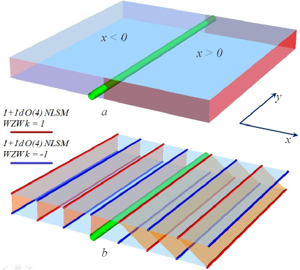
Figure 2: A vison line in a 3d SPT phase. $(a)$, the two 2d boundaries exposed after cutting the SPT phase at $z=0$. $A(x)$ in Eq. 23 has a domain wall at $x=0$. $(b)$, the two boundaries can both be viewed as coupled 1d wires that are described by 1+1d O(4) NLSM with WZW term at level $k=\pm 1$ (Eq. 32).

Every term in the lattice Hamiltonian must only have even powers of $S^{x}$ and $S^{y}$ to protect the $Z_{2}\times Z_{2}^{T}$ symmetry. Thus we can consistently couple $S^{x}$ and $S^{y}$ to a $Z_{2}$ gauge theory: $H_{g}=\sum_{i,j}-t\sigma^{z}_{ij}S^{a}_{i}S^{b}_{j}+\cdots$ ($a,b=x,y$). With this coupling on the lattice, $n^{b}$ with $b=4,5$ are coupled to the same $Z_{2}$ gauge field

The simple half-vortex line picture in the previous examples is not totally applicable here, because there is no U(1) degree of freedom that can form a vortex around the vison loop. Thus let us instead consider the following structure: Cut the system open in the XY plane at $z=0$, which will expose two boundaries (Fig. 2$a$). Both boundaries must have nontrivial spectrum, and they are both described by a 2+1d NLSM with O(5) vector $\vec{n}$ plus a Wess-Zumino-Witten (WZW) term at level $k=\pm 1$ respectively:

$$\mathcal{S}_{\alpha}=\int d^{2}xd\tau\frac{1}{g}(\partial_{\mu}\vec{n}_{\alpha})^{2}$$ (15)

$$\pm \int d^{3}x\int_{0}^{1}du\frac{2\pi i}{\Omega_{4}}\epsilon_{abcde}n^{a}_{\alpha}\partial_{x}n^{b}_{\alpha}\partial_{y}n^{c}_{\alpha}\partial_{u}n^{d}_{\alpha}\partial_{\tau}n^{e}_{\alpha},$$ (17)

Here $\alpha=1,2$ denotes the top and bottom boundaries exposed. The O(5) WZW term has level $k=1$ for top boundary ($\alpha=1$), and $k=-1$ for bottom boundary ($\alpha=2$) respectively. $\vec{n}_{\alpha}(x,y,\tau,u)$ is an extension of the space-time configuration $\vec{n}_{\alpha}(x,y,\tau)$ that satisfies $\vec{n}_{\alpha}(x,y,\tau,0)=(0,0,0,0,1)$, and $\vec{n}_{\alpha}(x,y,\tau,1)=\vec{n}_{\alpha}(x,y,\tau)$. The boundary WZW term can be derived from the bulk $\Theta-$term in Eq. 1, because when $\Theta=2\pi$, the 3+1d bulk $\Theta-$term can be written as 2+1d WZW terms at boundaries $z=L$ and $z=0$: $\Theta-\mathrm{term}=\mathrm{WZW}_{L,k=1}+\mathrm{WZW}_{0,k=-1}$.

The symmetry of Eq. 17 needs to be reduced to the physical symmetry. Let us assume the system energetically favors $n^{4}$ over $n^{5}$, so we can integrate out $n^{5}_{1}$ and $n^{5}_{2}$ from Eq. 17 to obtain an effective action for O(4) vectors $\vec{n}_{\alpha}=(n^{1}_{\alpha},n^{2}_{\alpha},n^{3}_{\alpha},n^{4}_{\alpha})$. If the system preserves the $Z_{2}$ symmetry, then the expectation values $\langle n^{5}_{1}\rangle=\langle n^{5}_{2}\rangle=0$. Now after integrating out $n^{5}_{\alpha}$, Eq. 17 is reduced to two O(4) NLSMs with a $\Theta-$term at $\Theta=\pm\pi$:

$$\mathcal{S} = \int d^{3}x\frac{1}{g}(\partial_{\mu}\vec{n}_{\alpha})^{2}$$ (18)

$$\pm \int d^{3}x\frac{i\pi}{12\pi^{2}}\epsilon_{abcd}\epsilon_{\mu\nu\rho}n^{a}_{\alpha}\partial_{\mu}n^{b}_{\alpha}\partial_{\nu}n^{c}_{\alpha}\partial_{\rho}n^{d}_{\alpha}.$$ (20)

Here $\Theta=\pi$ on the top boundary (or $-\pi$ on the bottom boundary) is protected by the $Z_{2}$ symmetry. Detailed calculation of the $\Theta-$term at the boundary can be found in Ref. Vishwanath and Senthil (2013); Xu (2013).

Now let us reglue the two boundaries together, by turning on the following coupling:

$$\mathcal{S}_{c} = \int d^{2}xd\tau\ \sum_{a=1}^{3}Bn^{a}_{1}(x,\tau)n^{a}_{2}(x,\tau)$$ (21)

$$+ \sum_{b=4,5}A(x)n^{b}_{1}(x,\tau)n^{b}_{2}(x,\tau).$$ (23)

The coupling constant $A(x)$ has a 1d domain wall at $x=z=0$: $A(x)<0\ \mathrm{for}\ x<0$, $A(x)>0\ \mathrm{for}\ x>0$. For the entire XY plane $B<0$. This inter-boundary coupling corresponds to inserting a vison loop in the XY plane along the $y-$axis at $x=z=0$. For the half plane $z=0,x<0$, we can identify $\vec{n}_{1}(x,\tau)=\vec{n}_{2}(x,\tau)=\vec{n}(x,\tau)$, and eventually the effective 2d action in this half-plane is an ordinary O(4) NLSM with no $\Theta-$term. In the opposite half-plane $z=0,x>0$, since $A(x)>0$, we have $(n^{1}_{1},n^{2}_{1},n^{3}_{1},n^{4}_{1})=(n^{1}_{2},n^{2}_{2},n^{3}_{2},-n^{4}_{2})=\vec{n}$, and the effective action for $\vec{n}$ in the half-plane $x>0$ is an O(4) NLSM with $\Theta=2\pi$:

$$\mathcal{S}_{x>0} = \int d^{3}x\frac{1}{g}(\partial_{\mu}\vec{n})^{2}$$ (24)

$$+ \int d^{3}x\frac{i2\pi}{12\pi^{2}}\epsilon_{abcd}\epsilon_{\mu\nu\rho}n^{a}\partial_{\mu}n^{b}\partial_{\nu}n^{c}\partial_{\rho}n^{d}.$$ (26)

Now the vison loop can be viewed as a 1d domain wall of $\Theta$ between $\Theta=0$ at $x<0$, and $\Theta=2\pi$ at $x>0$. Although both sides of the domain wall can be driven into a 2d gapped disordered phase without degeneracy, the domain wall must have nontrivial spectrum. Using the analysis in Ref. Xu and Ludwig (2011), if both sides of the domain wall are gapped, this domain wall (vison loop) is described by a 1+1d O(4) NLSM with a WZW term at level-1:

$$\mathcal{S} = \int dyd\tau\ \frac{1}{g}(\partial_{\mu}\vec{n})^{2}$$ (27)

$$+ \int d^{2}x\int_{0}^{1}du\frac{i2\pi}{12\pi^{2}}n^{a}\partial_{\mu}n^{b}\partial_{\nu}n^{c}\partial_{\rho}n^{d}\epsilon_{abcd}\epsilon_{\mu\nu\rho}.$$ (29)

It is well-known that this theory flows to a stable 1+1d SU(2)₁ conformal field theory fixed point under renormalization group Witten (1984); Knizhnik and Zamolodchikov (1984), if the system has a full SO(4) symmetry. In our case, although the symmetry is much lower than SO(4), no linear term of $n^{a}$ is allowed by symmetry. Any bilinear term of $n^{a}$, even if it is relevant at the SU(2)₁ fixed point, will eventually lead to spontaneous symmetry breaking and degenerate ground states.

We seek for a more physical picture for the formal calculation above. Before regluing the boundaries together, the boundaries are described by O(4) NLSM with $\Theta=\pm\pi$ (Eq. 20). This theory can be viewed as coupled 1d wires along $y$ direction Senthil and Fisher (2005), and every wire is a 1+1d O(4) NLSM with a WZW term at level $k=\pm 1$ (Fig. 2$b$):

$$\mathcal{S}_{\alpha=1,2,x=j}=\int dyd\tau\ \frac{1}{g}(\partial_{\mu}\vec{n}_{\alpha})^{2}\pm$$ (30)

(31)

$$\frac{i\pi(-1)^{j}}{12\pi^{2}}\int dyd\tau\int^{1}_{0}du\ \epsilon_{abcd}\epsilon_{\mu\nu\rho}n^{a}_{\alpha}\partial_{\mu}n^{b}_{\alpha}\partial_{\nu}n^{c}_{\alpha}\partial_{\rho}n^{d}_{\alpha}.$$ (32)

If a direct inter-wire coupling $\sum_{\alpha=1,2}\sum_{j}\vec{n}(x=j,y,\tau)_{\alpha}\cdot\vec{n}(x=j+a,y,\tau)_{\alpha}$ is turned on ($a$ is the distance between nearest neighbor wires), each boundary reduces to the 2+1d O(4) NLSM with $\Theta=\pm\pi$ (Eq. 20) Senthil and Fisher (2005).

Now we glue the two boundaries together with a domain wall of $A(x)$. In the half plane $x<0$, since $\vec{n}_{1}=\vec{n}_{2}=\vec{n}$, two wires on top and bottom boundaries would trivially gap out due to their coupling with each other (their WZW terms cancel each other); however, on the other half plane $x>0$, due to the opposite sign of inter-boundary coupling, the WZW term of the top boundary wire $x=j$ will cancel the WZW term of the bottom boundary wire $x=j+a$. Thus at the domain wall $x=0$, there is one 1d wire left which is not gapped by coupling with other wires.

This picture is very analogous to coupling two spin-1/2 chains together. Let us consider two spin-1/2 Heisenberg chains along $x$ direction: $H=\sum_{\alpha=1,2}\sum_{j}\vec{S}_{j,\alpha}\vec{S}_{j+1,\alpha}$. At $x<0$ we couple the two chains antiferromagnetically: $H^{\prime}=\sum_{j}J^{\prime}\vec{S}_{j,1}\cdot\vec{S}_{j,2}$, while for $x>0$ we couple the two chains ferromagnetically: $H^{\prime}=\sum_{j}-J^{\prime}\vec{S}_{j,1}\cdot\vec{S}_{j,2}$. Then the half-line $x<0$ can be viewed as a trivial spin-0 chain, while for $x>0$ it is the Haldane phase of a spin-1 chain. Then at the origin $x=0$ it is guaranteed to have a dangling spin-1/2 doublet.

The same kind of analysis and conclusion can be applied to the phase 2 of SPT phase with $Z_{2}\times Z_{2}^{T}$ symmetry, where the O(5) vector $\vec{n}$ transforms as $Z_{2}:n^{1}\rightarrow n^{1},\ n^{b}\rightarrow-n^{b},b=2\cdots 5$; $Z_{2}^{T}:n^{a}\rightarrow-n^{a},a=1\cdots 5$. The only difference from phase 1 is that, in this case we need to couple $n^{b}$ with $b=2-5$ to the same $Z_{2}$ gauge field.

Example 4: Point defect in 2d SPT phase

Let us now briefly discuss 2d SPT phases. A 2d SPT phase must have trivial spectrum in the bulk, but gapless or degenerate spectrum on its 1d boundary. But studies on quantum spin Hall insulator have suggested that if a point defect is created in a 2d SPT, this point defect might also change the spectrum. For example, if a quantum spin Hall insulator is coupled to a $Z_{2}$ gauge field, then the vison excitation of this $Z_{2}$ gauge field must carry a Kramers doublet Ran et al. (2008); Qi and Zhang (2008).

Here we argue that similar effect also occurs generally in 2d SPT phases. For instance, let us consider 2d bosonic SPT phase with $U(1)\rtimes Z_{2}^{T}$ symmetry, which is a bosonic version of QSH insulator. This SPT phase is described by a 2+1d O(4) NLSM with $\Theta=2\pi$ Xu and Senthil (2013) which involves a four component vector $\vec{n}=(n^{1},n^{2},n^{3},n^{4})$. $n^{1}+in^{2}$ is a boson rotor that transforms under U(1), and $n^{2},n^{3},n^{4}$ all change sign under $Z_{2}^{T}$. Let us couple $n^{1}$ and $n^{2}$ to a $Z_{2}$ gauge field, and consider a vison at the origin of the 2d system. Then this vison is bound with a half-vortex of $b$, which leads to a $0+1d$ O(2) NLSM for $n^{3}$ and $n^{4}$ with $\Theta_{0d}=\pi$ at the origin: $S=\int d\tau\frac{i\pi}{2\pi}\epsilon_{ab}n^{a}\partial_{\tau}n^{b}$, $a,b=3,4$. This $0+1d$ model can be solved exactly, and its ground state is two fold degenerate, which is precisely a Kramers doublet. This degeneracy is again protected by time-reversal symmetry. Thus a vison excitation in a $Z_{2}-$gauged bosonic quantum spin Hall insulator has the same behavior as the fermionic QSH state.

If we break the U(1) symmetry down to $Z_{2}$ (consider 2d SPT phase with $Z_{2}\times Z_{2}^{T}$ symmetry), we can still couple $n^{1}$ and $n^{2}$ to a $Z_{2}$ gauge field. Now a lower dimensional version of Fig. 2 allows us to study the spectrum of the vison in the system, and the vison will still be two fold degenerate. The vison spectrum in this case can also be understood using the “decorated domain wall” construction of SPT phases discussed in Ref. Chen et al. (2013). In the 2d $Z_{2}\times Z_{2}^{T}$ SPT, a domain wall of the $Z_{2}$ symmetry is a 1d SPT phase with $Z_{2}^{T}$ symmetry, and after coupling the $Z_{2}$ part to a $Z_{2}$ gauge field, a vison is the 0d boundary of the 1d SPT, thus it must be a 2-fold degenerate Kramers doublet. However, none of the defects in the previous cases discussed in this paper can be analyzed using the decorated domain wall construction. Our studies based on effective field theory are more general.

In summary, we study the defects in SPT phases introduced by $Z_{2}$ gauge field, and in all the cases discussed in this paper the defect (either line defect in 3d or point defect in 2d) has nontrivial spectrum. Our study not only reveals a new general property of SPT phases, it also suggests a possible way of classifying 3d $Z_{2}$ topological order enriched by symmetry, based on the spectrum of its vison line.

CX is supported by the Alfred P. Sloan Foundation, the David and Lucile Packard Foundation, Hellman Family Foundation, and NSF Grant No. DMR-1151208. ZB is supported by NSF DMR-1151208.

References

- Kane and Mele (2005a) C. L. Kane and E. J. Mele, Physical Review Letter 95, 226801 (2005a).
- Kane and Mele (2005b) C. L. Kane and E. J. Mele, Physical Review Letter 95, 146802 (2005b).
- Bernevig et al. (2006) B. A. Bernevig, T. L. Hughes, and S.-C. Zhang, Science 314, 1757 (2006).
- Moore and Balents (2007) J. E. Moore and L. Balents, Physical Review B 75, 121306(R) (2007).
- Fu et al. (2007) L. Fu, C. L. Kane, and E. J. Mele, Phys. Rev. Lett. 98, 106803 (2007).
- Roy (2009) R. Roy, Physical Review B 79, 195322 (2009).
- Chen et al. (2011) X. Chen, Z.-C. Gu, Z.-X. Liu, and X.-G. Wen, arXiv:1106.4772 (2011).
- Chen et al. (2012) X. Chen, Z.-C. Gu, Z.-X. Liu, and X.-G. Wen, Science 338, 1604 (2012).
- Senthil and Levin (2013) T. Senthil and M. Levin, Phys. Rev. Lett. 110, 046801 (2013).
- Levin and Stern (2012) M. Levin and A. Stern, Phys. Rev. B 86, 115131 (2012).
- Liu and Wen (2013) Z.-X. Liu and X.-G. Wen, Phys. Rev. Lett. 110, 067205 (2013).
- Lu and Vishwanath (2012) Y.-M. Lu and A. Vishwanath, Phys. Rev. B 86, 125119 (2012).
- Vishwanath and Senthil (2013) A. Vishwanath and T. Senthil, Phys. Rev. X 3, 011016 (2013).
- Xu (2013) C. Xu, Phys. Rev. B 87, 144421 (2013).
- Oon et al. (2012) J. Oon, G. Y. Cho, and C. Xu, arXiv:1212.1726 (2012).
- Xu and Senthil (2013) C. Xu and T. Senthil, arXiv:1301.6172 (2013).
- Wang and Senthil (2013) C. Wang and T. Senthil, arXiv:1302.6234 (2013).
- Chen et al. (2013) X. Chen, Y.-M. Lu, and A. Vishwanath, arXiv:1303.4301 (2013).
- Metlitski et al. (2013) M. A. Metlitski, C. L. Kane, and M. P. A. Fisher, arXiv:1302.6535 (2013).
- Ye and Wen (2012) P. Ye and X.-G. Wen, arXiv:1212.2121 (2012).
- Ye and Wen (2013) P. Ye and X.-G. Wen, arXiv:1303.3572 (2013).
- Ran et al. (2009a) Y. Ran, Y. Zhang, and A. Vishwanath, Nature Physics 5, 298 (2009a).
- Ran et al. (2009b) Y. Ran, Y. Zhang, and A. Vishwanath, Phys. Rev. B 79, 245331 (2009b).
- Xu and Ludwig (2011) C. Xu and A. W. W. Ludwig, arXiv:1112.5303 (2011).
- Lieb et al. (1961) E. H. Lieb, T. D. Schultz, and D. C. Mattis, Ann. Phys. 16, 407 (1961).
- Witten (1984) E. Witten, Commun. Math. Phys. 92, 455 (1984).
- Knizhnik and Zamolodchikov (1984) V. G. Knizhnik and A. B. Zamolodchikov, Nucl. Phys. B 247, 83 (1984).
- Senthil and Fisher (2005) T. Senthil and M. P. A. Fisher, Phys. Rev. B 74, 064405 (2005).
- Ran et al. (2008) Y. Ran, A. Vishwanath, and D.-H. Lee, Phys. Rev. Lett. 101, 086801 (2008).
- Qi and Zhang (2008) X.-L. Qi and S.-C. Zhang, Phys. Rev. Lett. 101, 086802 (2008).