First observational constraints on tensor non-Gaussianity sourced by primordial magnetic fields from cosmic microwave background

Abstract

Primordial magnetic fields (PMFs) create a large squeezed-type non-Gaussianity in tensor perturbation, which generates non-Gaussian temperature fluctuations in the cosmic microwave background (CMB). We for the first time derive an observational constraint on such a tensor non-Gaussianity from observed CMB maps. Analyzing temperature maps of the WMAP 7-year data, we find that such a tensor non-Gaussianity is consistent with zero. This gives an upper bound on PMF strength smoothed on $1~{}{\rm Mpc}$ as $B_{1~{}\rm Mpc}<3.1~{}{\rm nG}$ at $95\%$ C.L.

I Introduction

Primordial non-Gaussianity is a powerful probe of inflationary models, and various aspects of their property, e.g., amplitude and scale dependence, have been investigated from a diversity of cosmological and astrophysical observables. To date, methods to estimate parameters characterizing non-Gaussianity in primordial perturbations from the cosmic microwave background (CMB) have been extensively investigated by many authors Komatsu and Spergel (2001); Eriksen et al. (2004); Smith and Zaldarriaga (2011); Yadav et al. (2007, 2008); Hikage et al. (2008); Matsubara (2010); Bennett et al. (2013); Shiraishi et al. (2013). Some specific types of non-Gaussianity have already been constrained by observed data, e.g., $f_{\rm NL}^{\rm loc}=2.7\pm 5.8$, $f_{\rm NL}^{\rm eq}=-42\pm 75$, and $f_{\rm NL}^{\rm orth}=-25\pm 39$ (68% C.L.) Ade et al. (2013a) (for scale-dependent non-Gaussianities, see Ref. Becker and Huterer (2012)).

These bounds have been estimated under an assumption that the primordial non-Gaussianity arises from the scalar perturbations. On the other hand, there exist various models for the early Universe which predict non-Gaussianities associated with not only scalar mode but also vector and tensor modes Shiraishi et al. (2011a); Maldacena and Pimentel (2011); Soda et al. (2011); Shiraishi et al. (2011b); Gao et al. (2011, 2013). Despite that many attempts have been made so far to constrain primordial non-Gaussianities, those in vector and tensor perturbations predicted by these models have yet to be constrained. Provided predictions from theoretical models and precise data from current CMB observations, we believe that it is timely to investigate constraints on non-Gaussianities in perturbations other than scalar ones. Among various theoretical models, we in this paper focus on the electromagnetic field in the early Universe as a mechanism to generate vector and tensor non-Gaussianities Shiraishi et al. (2010a); Kahniashvili and Lavrelashvili (2010); Shiraishi et al. (2011c).

By cosmological observations of galaxies, cluster of galaxies, and cosmic rays, the existence of large-scale magnetic fields at the present Universe is supported (see, e.g., Refs. Wolfe et al. (2008); Bernet et al. (2008)). There have been a number of studies in which vector fields that exist during inflation are examined as sources for the observed magnetic fields Grasso and Rubinstein (2001); Widrow (2002); Bamba and Sasaki (2007); Martin and Yokoyama (2008). However, due to the problems of backreaction and strong dynamics, it has been in general very difficult to construct a consistent model of magnetogenesis via primordial vector fields Demozzi et al. (2009); Demozzi and Ringeval (2012); Suyama and Yokoyama (2012); Fujita and Mukohyama (2012); Ringeval et al. (2013). While these theoretical considerations strongly restrict model building, phenomenological approaches to constrain primordial magnetogenesis are also important. Specifically, through impacts on the CMB anisotropy, properties of primordial magnetic fields (PMFs), which are assumed to be generated from primordial vector fields, can be constrained. For example, observational constraints on the amplitude of PMFs as well as its scale dependence can be obtained by the CMB power spectra alone (for current bounds, see, e.g., Refs. Shaw and Lewis (2012); Yadav et al. (2012); Paoletti and Finelli (2013); Ade et al. (2013b)).

Assuming that the field strength of PMFs has a Gaussian distribution, their energy-momentum tensor creates all types of perturbations, which are highly non-Gaussian due to the quadratic dependence on the field strength Brown and Crittenden (2005); Seshadri and Subramanian (2009); Caprini et al. (2009); Cai et al. (2010); Shiraishi et al. (2010a); Kahniashvili and Lavrelashvili (2010); Trivedi et al. (2010, 2012); Shiraishi et al. (2011c, d); Shiraishi et al. (2012); Trivedi et al. (2014); Shiraishi (2013). This leads to non-Gaussian CMB anisotropies and suggests that higher order correlation functions or polyspectra of the CMB anisotropy beyond the power spectrum should also be informative in probing PMFs. On the basis of this concept, this paper newly explores an observational constraint on the PMF strength by evaluating the magnitude of non-Gaussianity in the CMB temperature anisotropies.

In the case of PMF, the tensor non-Gaussianity, which becomes prominent in the squeezed limit, dominates over the scalar one Shiraishi et al. (2012), and hence, non-Gaussian temperature fluctuations mainly have information of the tensor mode. Since CMB tensor-mode fluctuations generated from PMFs have unique features and are distinct from CMB signals from ordinary scalar perturbations in inflationary Universe, a nontrivial constraint is expected to be obtained. In this sense, this work corresponds to a first attempt to constrain a tensor non-Gaussianity from CMB data. This is also another motivation of this paper.

This paper is organized as follows. In the next section, we summarize the tensor non-Gaussianity originating from PMFs. In Sec. III, after performing some validation tests of our bispectrum estimator and data treatments, we put limits on the magnetic tensor bispectrum from the observed temperature maps of the WMAP 7-year result Komatsu et al. (2011); Larson et al. (2011); Jarosik et al. (2011); Gold et al. (2011), which we translate into constraints on the amplitude of PMFs. The final section is devoted to summary and discussion.

II Tensor non-Gaussianity generated from PMFs

First, we briefly summarize the mechanism of PMFs to generate CMB temperature fluctuations and its signatures in observed CMB bispectrum. After PMFs are produced and stretched beyond the horizon during inflation, the anisotropic stress of PMFs contributes to the source term in the Einstein equation and supports the growth of curvature and tensor perturbations even on superhorizon scales until neutrino decoupling. However, subsequent to neutrino decoupling, finite anisotropic stress fluctuations in neutrinos cancel out the magnetic anisotropic stress fluctuations, and therefore, the enhancement of metric perturbations ceases. The resultant curvature and tensor perturbations produce CMB anisotropies, which are called passive-mode fluctuations Shaw and Lewis (2010).

Let us denotes the initial perturbations of the transverse-traceless (TT) part of the metric as $\delta g_{ij}^{\rm TT}/a^{2}=\int\frac{d^{3}{\bf k}}{(2\pi)^{3}}\sum_{\lambda=\pm 2}h_{\bf k}^{(\lambda)}e_{ij}^{(\lambda)}(\hat{\bf k})e^{i{\bf k}\cdot{\bf x}}$, where $\lambda$ denotes the helicity and $e_{ij}^{(\lambda)}(\hat{\bf k})$ is the basis of TT tensors obeying $e_{ij}^{(\lambda)}(\hat{\bf k})e_{ij}^{(\lambda^{\prime})}(\hat{\bf k})=2\delta_{\lambda,-\lambda^{\prime}}$ and $e_{ij}^{(\lambda)*}(\hat{\bf k})=e_{ij}^{(-\lambda)}(\hat{\bf k})=e_{ij}^{(\lambda)}(-\hat{\bf k})$ Shiraishi et al. (2011a). The initial condition of CMB fluctuations is determined by $h^{(\lambda)}_{\bf k}$, which are estimated as Shaw and Lewis (2010)

$$h_{\bf k}^{(\lambda)} \approx -1.8\frac{\ln(T_{B}/T_{\nu})}{4\pi\rho_{\gamma,0}}e_{ij}^{(-\lambda)}(\hat{\bf k})$$ (1)

$$\times\int\frac{d^{3}{\bf k^{\prime}}}{(2\pi)^{3}}B_{i}({\bf k^{\prime}})B_{j}({\bf k}-{\bf k^{\prime}})~{},$$

where $T_{B}$ and $T_{\nu}$ denote the energy scales at PMF creation and neutrino decoupling, respectively, and $\rho_{\gamma,0}$ is the present photon energy density. Supposing that PMFs $B_{i}$ are quantum-mechanically created and the probability distribution of their field strength obeys pure Gaussian statistics as is the case in majority of models, $h_{\bf k}^{(\lambda)}$, which is proportional to the PMF anisotropic stress fluctuations, becomes highly non-Gaussian fields obeying the chi-square distribution due to the quadratic dependence on the Gaussian PMFs. Owing to the local form of Eq. (1), the bispectrum of gravitational waves [$\Braket{\prod_{n=1}^{3}h_{{\bf k}_{n}}^{(\lambda_{n})}}$ or $\Braket{\prod_{n=1}^{3}h_{\ell_{n}m_{n}}^{(\lambda_{n})}(k_{n})}$ in Eq. (4)] is amplified in the squeezed limit ($k_{1}\approx k_{2}\gg k_{3}$ or $\ell_{1}\approx\ell_{2}\gg\ell_{3}$) if the PMF power spectrum is nearly scale invariant Shiraishi et al. (2011c); Shiraishi et al. (2012).

The CMB temperature anisotropies for given direction $\hat{\bf n}$ are quantified via the spherical harmonics expansion as $\frac{\Delta T(\hat{\bf n})}{T}=\sum_{\ell m}a_{\ell m}Y_{\ell m}(\hat{\bf n})$. Using a harmonic-space representation, $h_{\bf k}^{(\lambda)}=\sum_{\ell m}h_{\ell m}^{(\lambda)}(k){}_{-\lambda}Y_{\ell m}(\hat{\bf k})$, the CMB bispectrum is formed as Shiraishi et al. (2010b, 2011a)

$$\Braket{\prod_{n=1}^{3}a_{\ell_{n}m_{n}}} = \left[\prod_{n=1}^{3}(-i)^{\ell_{n}}\int\frac{k_{n}^{2}dk_{n}}{2\pi^{2}}{\cal T}_{\ell_{n}}(k_{n})\right]$$ (4)

$$\times\sum_{\lambda_{1},\lambda_{2},\lambda_{3}=\pm 2}\Braket{\prod_{n=1}^{3}h_{\ell_{n}m_{n}}^{(\lambda_{n})}(k_{n})}$$

$$= \left(\begin{array}[]{ccc}\ell_{1}&\ell_{2}&\ell_{3}\\ m_{1}&m_{2}&m_{3}\end{array}\right)B_{\ell_{1}\ell_{2}\ell_{3}}~{},$$

where ${\cal T}_{\ell}(k)$ is the temperature transfer function of the tensor mode involving the amplification for $\ell\lesssim 100$ by the tensor-mode Integrated Sachs-Wolfe (ISW) effect Pritchard and Kamionkowski (2005). The transfer function determines the shapes of the CMB bispectrum; thus, the tensor-mode magnetic $B_{\ell_{1}\ell_{2}\ell_{3}}$ under examination is less correlated with the usual scalar local-type one, even if their primordial Fourier-space bispectra resemble each other Shiraishi et al. (2012); Shiraishi (2013). According to Ref. Shiraishi et al. (2012), under the presence of PMFs, the tensor mode dominates over total signal of the CMB bispectrum at the WMAP angular resolution ($\ell\lesssim 500$), and the contributions of scalar and vector modes are negligible. Therefore, in our bispectrum estimation, we take into account the signals coming from the tensor non-Gaussianity (1) alone. Note that $B_{\ell_{1}\ell_{2}\ell_{3}}$ is proportional to the magnetic field strength to the sixth power.

In what follows, we obey the conventional parametrization for the power spectrum of PMFs as

$$\Braket{B^{i}({\bf k})B_{j}({\bf k^{\prime}})} = (2\pi)^{3}\frac{P_{B}(k)}{2}P^{i}_{~{}j}(\hat{\bf k})\delta^{(3)}({\bf k}+{\bf k^{\prime}})~{},$$ (5)

$$P_{B}(k) = \frac{(2\pi)^{n_{B}+5}B_{1~{}\rm Mpc}^{2}}{\Gamma(\frac{n_{B}+3}{2})(\frac{2\pi}{1~{}\rm Mpc})^{n_{B}+3}}k^{n_{B}},$$ (6)

where $P^{i}_{~{}j}(\hat{\bf k})\equiv\delta^{i}_{~{}j}-\hat{k}^{i}\hat{k}_{j}$, $n_{B}$ and $B_{1~{}\rm Mpc}$ are the divergence-free projection tensor, the PMF spectral index, and the PMF strength smoothed on $1~{}\rm Mpc$ scale, respectively. In the next section, we constrain the amplitude of bispectrum given by

$$A\equiv\left(\frac{B_{1~{}\rm Mpc}}{3~{}{\rm nG}}\right)^{6}\propto B_{\ell_{1}\ell_{2}\ell_{3}}~{},$$ (7)

under an assumption of the generation of PMFs at the GUT scale ($T_{B}/T_{\nu}=10^{17}$) and nearly scale-invariant shapes of the PMF power spectrum ($n_{B}=-2.9$). Note that theoretically $A$ should take a positive value.

In the Planck bispectrum analysis Ade et al. (2013a), a non-Gaussianity parameter of the Legendre-polynomial bispectra (the so-called $c_{2}$), parametrizing the size of magnetic bispectrum of the passive scalar mode with $n_{B}=-2.9$ and $T_{B}/T_{\nu}=10^{17}$, namely $c_{2}\approx-2A$, was constrained, and the corresponding limit is $A=-1.9\pm 13.9$ (68% C.L.) or $B_{1~{}\rm Mpc}<5.2~{}{\rm nG}$ (95% C.L.) Shiraishi et al. (2013). In the next section, we obtain more stringent constraints even from the WMAP data since the most dominant contribution comes from the tensor-mode bispectrum under examination, which was not included in the previous analysis Ade et al. (2013a). We note that there are other bounds on PMFs from the CMB power spectra, where the so-called magnetic compensated mode Paoletti et al. (2009); Shaw and Lewis (2010) is included and/or $n_{B}$ is treated as a free parameter: Planck gives $B_{1~{}\rm Mpc}<3.4~{}{\rm nG}$ and $n_{B}<0$ Ade et al. (2013b), and SPT gives $B_{\rm 1~{}Mpc}<3.5~{}{\rm nG}$ Paoletti and Finelli (2013).

III Observational limits

Given a theoretical template of $B_{\ell_{1}\ell_{2}\ell_{3}}$ for a specific theoretical model, we can in general construct an optimal estimator of the amplitude of the bispectrum of primordial perturbations Komatsu et al. (2005); Yadav et al. (2008). An optimal cubic estimator for the amplitude of bispectrum can be approximated as

$$\hat{A} = \frac{1}{6{\mathcal{N}}}\sum_{\ell_{i}m_{i}}\left(\begin{array}[]{ccc}\ell_{1}&\ell_{2}&\ell_{3}\\ m_{1}&m_{2}&m_{3}\end{array}\right)B_{\ell_{1}\ell_{2}\ell_{3}}^{A=1}$$ (11)

$$\times\left[\prod_{n=1}^{3}\frac{a_{\ell_{n}m_{n}}}{C_{\ell_{n}}}-3\frac{\Braket{a_{\ell_{1}m_{1}}a_{\ell_{2}m_{2}}}_{\rm MC}}{C_{\ell_{1}}C_{\ell_{2}}}\frac{a_{\ell_{3}m_{3}}}{C_{\ell_{3}}}\right],$$

where $B_{\ell_{1}\ell_{2}\ell_{3}}^{A=1}$ is the template bispectrum for the PMF model being normalized with $A=1$, the bracket denotes the ensemble average of (Gaussian) Monte-Carlo realizations, and $\mathcal{N}$ is the normalization factor equal to the Fisher matrix:

$${\cal N} \equiv \sum_{\ell_{1}\ell_{2}\ell_{3}}\frac{(B_{\ell_{1}\ell_{2}\ell_{3}}^{A=1})^{2}}{6C_{\ell_{1}}C_{\ell_{2}}C_{\ell_{3}}}~{}.$$ (12)

This estimator form is derived under the so-called diagonal covariance approximation where numerically unfeasible computations of inverse of the covariance matrix are avoided by a simple replacement $(C^{-1}a)_{\ell}\to a_{\ell}/C_{\ell}$. Practically, the bispectrum estimations based on this approximate form and the simple recursive inpainting technique for regions covered by mask retain optimality (with error bars that agree with the optimal ones derived from the Fisher matrix within 5%), and hence, it has been adopted in the Planck analysis Ade et al. (2013a). Note that this form automatically involves relevant experimental features, i.e., beam, partial sky mask, and anisotropic noise, as $B_{\ell_{1}\ell_{2}\ell_{3}}=b_{\ell_{1}}b_{\ell_{2}}b_{\ell_{3}}B_{\ell_{1}\ell_{2}\ell_{3}}^{\rm theory}$ and $C_{\ell}=b_{\ell}^{2}C_{\ell}^{\rm theory}+N_{\ell}$, with $b_{\ell}$ and $N_{\ell}$ denoting beam transfer function and noise spectrum.

The form (11) indicates that to obtain $\hat{A}$ from a single realization, a direct implementation requires ${\cal O}(\ell_{\rm max}^{5})$ arithmetics (as is the case in non-Gaussian map creation mentioned in Sec. III.1), where $\ell_{\rm max}$ is the maximum multipole. For $\ell_{\rm max}\sim 1000$, required computational time is enormous. In the literature of the so-called KSW approach Komatsu et al. (2003); Senatore et al. (2010); Creminelli et al. (2006); Yadav et al. (2008), a factorized estimator form has been found for the case of the standard scalar non-Gaussianity where the angle dependence is removed, since the dependence on $(\ell_{1},m_{1})$, $(\ell_{2},m_{2})$, and $(\ell_{3},m_{3})$ can be separated from one another. On the other hand, in the tensor case, due to complicated spin dependence, different multipoles are tangled with one another and there is no way to reduce numerical operations in the same manner as the KSW approach. In this paper, we straightforwardly perform ${\cal O}(\ell_{\rm max}^{5})$ arithmetics in estimator computations; then to prevents us from taking too much computational time, let us stop summations at $\ell_{\rm max}=100$. In our PMF case, the signal-to-noise ratio is almost saturated at $\ell\simeq 100$ Shiraishi et al. (2012); thus, we believe that by choosing such small $\ell_{\rm max}$, constraints on $A$ do not change so much in comparison with analyses at the WMAP resolution $\ell_{\rm max}\simeq 500$.

A summary of our analysis and treatment of the data set are as follows. In Sec. III.2, we place observational limits on the magnetic bispectrum using the coadded temperature maps from the WMAP 7-year observation at V and W bands Jarosik et al. (2011); Gold et al. (2011). We then compare the constraints from both (not foreground-cleaned) raw and foreground-cleaned data. Prior to it, in Sec. III.1, we check the validity of our estimator by using simulated non-Gaussian maps originating from known magnetic bispectrum. In these works, for error estimations and linear term computations, we use 500 simulated Gaussian maps. Taking into account experimental uncertainties, in these maps, we include an anisotropic noise component. Furthermore, to reduce effects of residual foregrounds, we apply the KQ75y7 mask recommended by the WMAP team Gold et al. (2011), whose sky coverage is $f_{\rm sky}=0.706$. After removing monopole and dipole components, the masked regions are inpainted by means of the recursive inpainting procedure adopted in the Planck analysis Ade et al. (2013a). Our pixel-space computations are based on a resolution $N_{\rm side}=512$ in the HEALPix pixelization scheme Gorski et al. (2005). The CMB signal power spectrum $C_{\ell}$ is computed using the CAMB code Lewis et al. (2000), assuming a concordance flat power-law $\Lambda$CDM model with the mean cosmological parameters from the WMAP 7-year data alone Komatsu et al. (2011). Our beam transfer function and anisotropic noise component are generated by coadding the data in the V and W band channels by means of the WMAP-team method Komatsu et al. (2009).

III.1 Validation tests using simulated maps

Before moving to the actual data analysis, we check the validity of our bispectrum estimations mentioned above using simulated non-Gaussian maps with known PMF bispectrum. More specifically, we generate 50 realizations of non-Gaussian CMB temperature maps assuming $A=3.50$, which corresponds to $\sim 3\sigma$ significance and compare the estimator $\hat{A}$ of Eq. (11) from these realizations with the input $A$.

According to Refs. Fergusson et al. (2010); Hanson et al. (2009); Curto et al. (2011), given a power spectrum $C_{\ell}$ and bispectrum $B_{\ell_{1}\ell_{2}\ell_{3}}$, a random realization of CMB temperature anisotropy $a_{\ell m}$ can be approximately given as

$$a_{\ell m} \equiv a_{\ell m}^{\rm G}+a_{\ell m}^{\rm NG}~{},$$ (13)

$$a_{\ell_{1}m_{1}}^{\rm NG} = \frac{1}{6}\left[\prod_{n=2}^{3}\sum_{\ell_{n}m_{n}}\frac{a_{\ell_{n}m_{n}}^{{\rm G}*}}{C_{\ell_{n}}}\right]$$ (16)

$$\times\left(\begin{array}[]{ccc}\ell_{1}&\ell_{2}&\ell_{3}\\ m_{1}&m_{2}&m_{3}\end{array}\right)B_{\ell_{1}\ell_{2}\ell_{3}}~{}.$$

Here, $a_{\ell m}^{\rm G}$ is the Gaussian part of a realization whose variance is given by $\Braket{\prod_{n=1}^{2}a_{\ell_{n}m_{n}}^{\rm G}}=C_{\ell_{1}}(-1)^{m_{1}}\delta_{\ell_{1},\ell_{2}}\delta_{m_{1},-m_{2}}$, and $a_{\ell m}^{\rm NG}$ denotes the non-Gaussian part of the realization. In the same manner as the estimator computation, we stop summations at $\ell_{\rm max}=100$. This truncation is reasonable since, for $\ell\gtrsim 100$, the tensor bispectrum is highly damped and does not contribute to $a_{\ell m}^{\rm NG}$ as shown in Fig. 1. This also enables us to generate many non-Gaussian maps, despite the need for ${\cal O}(\ell_{\rm max}^{5})$ operations.

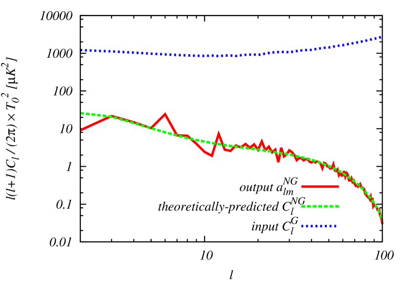
Figure 1: Angular power spectrum of a single non-Gaussian realization $a_{\ell m}^{\rm NG}$ with $A=3.50$ (red solid) generated from the input Gaussian power spectrum $C_{\ell}^{\rm G}$ (blue dotted). The consistency with the theoretically predicted power spectrum of $a_{\ell m}^{\rm NG}$ (green dashed) is confirmed. It is visually apparent that $a_{\ell m}^{\rm NG}$ decays rapidly at around $\ell=100$ due to the end of the ISW enhancement in the tensor bispectrum.

Mean values of $A$ computed from 50 non-Gaussian maps with $A=3.50$ and $1\sigma$ errors estimated from 500 Gaussian maps are summarized in Table 1. In these estimations, we assume two types of surveys: a full-sky noiseless “ideal” survey and a “WMAP-like” survey involving all experimental features of WMAP discussed above. It is verified from Table 1 that as expected, our estimator recovers the input value $A=3.50$ within error bars both in the ideal and WMAP-like surveys. Moreover, the resultant error bars are well consistent with the Fisher matrix values: $\delta A=1/\sqrt{f_{\rm sky}{\cal N}}=1.17$ (ideal) and $1.39$ (WMAP). These results show that our estimator retains optimality and support the validity of our computations.

	Ideal: $f_{\rm sky}=1$	WMAP: $f_{\rm sky}=0.706$
Average	3.54	3.86
$1\sigma$ error	1.13	1.36

Table 1: Mean values of $A$ obtained from 50 simulated non-Gaussian maps with the input value $A=3.50$, together with $1\sigma$ errors estimated from 500 Gaussian maps. We here compute the estimator assuming full-sky noiseless ideal and WMAP-like surveys. It is found that the mean values and the error bars reach the input value $3.50$ and the Fisher matrix values $1.17$ (ideal) and $1.39$ (WMAP), respectively.

III.2 WMAP results

Here we present our constraints from the WMAP7 (raw and foreground-cleaned) data, including experimental features (beam, noise and mask) and inpainted as mentioned above. Prior to estimating the amplitude of the magnetic bispectrum, we estimated $f^{\rm loc}_{\rm NL}$ with $\ell_{\rm max}=100$ from the foreground-cleaned data and found the $1\sigma$ bound: $(-1.0\pm 1.4)\times 10^{2}$, where this value is consistent with the corresponding results found from the figures in the literature Smith et al. (2009) and the error bar is also equal to the Fisher matrix value $1/\sqrt{f_{\rm sky}{\cal N}}$. This is another validation check of our data treatments.

In the PMF case, our final results from the raw and foreground-clean maps are, respectively, $A=-1.8\pm 1.4$ and $-1.5\pm 1.4$ (68% C.L.), indicating consistency with Gaussianity at $2\sigma$ regardless of the presence of foregrounds. Taking into account the foreground-cleaned result and a theoretical prior, $A\geq 0$, we find new upper limit on the PMF strength, namely, $B_{\rm 1~{}Mpc}<3.1$ nG at $95\%$ C.L. As expected, this is tighter than the passive scalar-mode constraint from Planck mentioned in Sec. II ($A=-1.9\pm 13.9$), owing to considering the tensor-mode contribution.

IV Summary and discussion

The origin of the observed large-scale magnetic fields is one of the most important and interesting issues in probe of the early Universe, and some researchers seek answers in the inflationary paradigm. In this paper, we have discussed an observational constraint on the seed magnetic field stretched by the inflationary expansion from the analysis of non-Gaussianities in CMB anisotropies. Signal of the Gaussian field strength of the PMF becomes largest on large scales via the enhancement of non-Gaussian tensor perturbations through the ISW effect.

We have analyzed the WMAP 7-year temperature maps and confirmed no evidence of squeezed-type tensor non-Gaussianity due to PMFs. Our constraint on the amplitude of the tensor non-Gaussianity leads to an upper bound on the PMF strength as $B_{\rm 1~{}Mpc}<3.1~{}{\rm nG}$ (95% C.L.). This result is not sensitive to the foregrounds. This value may be improved by considering impacts of polarizations Shiraishi (2013).

Aside from the issue on PMFs, this is a first challenge to constrain a primordial tensor non-Gaussianity from the CMB bispectrum. The tensor CMB bispectrum has spectral shapes quite distinct from the scalar one and leads to nontrivial constraints that have never seen in the scalar case. Unfortunately, the tensor bispectrum has a tangled multipole dependence, and the bispectrum estimator cannot be efficiently factorized as the KSW approach. In the present paper, we have performed ${\cal O}(\ell_{\rm max}^{5})$ huge amount of summations to compute the estimator in the brute-force way by focusing solely on large-scale signals up to $\ell_{\rm max}=100$. In other words, the brute-force method is not applicable to the data analysis with higher resolution, but it will be possible to access such small scales by means of a model-independent factorizable estimator Fergusson et al. (2010, 2012); Liguori et al. (2010); Fergusson and Shellard (2011); Shiraishi et al. (2014a); Fergusson (2014); Shiraishi et al. (2014b); Liguori et al. (2014). Probing tensor non-Gaussianity beyond $\ell_{\rm max}=100$ remains as a next challenging and exciting issue (although, of course, it is naturally expected that the constraints on the magnetic tensor bispectrum do not vary so much since the signal-to-noise ratio is already saturated at $\ell_{\rm max}=100$).