Calibrating C IV-based Black Hole Mass Estimators

Abstract

We present the single-epoch black hole mass estimators based on the C IV $\lambda$1549 broad emission line, using the updated sample of the reverberation-mapped AGNs and high-quality UV spectra. By performing multi-component spectral fitting analysis, we measure the C IV line widths (FWHM_CIV and line dispersion, $\sigma_{\rm CIV}$) and the continuum luminosity at 1350 Å ($L_{1350}$) to calibrate the C IV-based mass estimators. By comparing with the H$\beta$ reverberation-based masses, we provide new mass estimators with the best-fit relationships, i.e., $M_{\rm BH}\propto L_{1350}^{0.50\pm 0.07}\sigma_{\rm CIV}^{2}$ and $M_{\rm BH}\propto L_{1350}^{0.52\pm 0.09}{\rm FWHM}_{\rm CIV}^{0.56\pm 0.48}$. The new C IV-based mass estimators show significant mass-dependent systematic difference compared to the estimators commonly used in the literature. Using the published Sloan Digital Sky Survey QSO catalog, we show that the black hole mass of high-redshift QSOs decreases on average by $\sim 0.25$ dex if our recipe is adopted.

1. INTRODUCTION

Understanding the growth history of supermassive black holes (SMBHs) is one of the fundamental issues in studies of galaxy formation and evolution. The intimate connection between SMBHs and host galaxies is evidenced through empirical correlations between the masses of SMBHs (M_BH) and the overall properties of the host galaxy spheroids (e.g., Magorrian et al. 1998; Ferraresse & Merritt 2000; Gebhardt et al. 2000). The cosmic evolution of these scaling relationships has been investigated in the literature, where a tentative evolution has been reported utilizing observational approaches (e.g., Peng et al. 2006; Woo et al. 2006, 2008; Treu et al. 2007; Merloni et al. 2010; Bennert et al. 2010, 2011; Hiner et al. 2012; Canalizo et al. 2012). In order to provide better empirical constraints on the cosmic growth of SMBHs and its connection to galaxy evolution, reliable M_BH estimation at low and high redshifts is of paramount importance.

The M_BH can be determined for Type 1 AGN with the reverberation mapping (RM, Peterson 1993) method or the single-epoch (SE, Wandel et al. 1999) method under the virial assumption: $M_{\rm BH}=fR_{\rm BLR}{\varDelta V}^{2}/G$, where $G$ is the gravitational constant. The size of the broad-line region (BLR), $R_{\rm BLR}$, can be directly measured from RM analysis (e.g., Peterson et al 2004; Bentz et al. 2009; Denney et al. 2010; Barth et al. 2011b; Grier et al. 2012) or indirectly estimated from the monochromatic AGN luminosity measured from SE spectra based on the empirical BLR size-luminosity relation (Kaspi et al. 2000, 2005; Bentz et al. 2006, 2009, 2013). The line-of-sight velocity dispersion, $\varDelta V$, of BLR gas can be measured either from the broad emission line width in the rms spectrum (e.g., Peterson et al. 2004) obtained from multi-epoch RM data or in the SE spectra (e.g., Park et al. 2012b), while the virial factor, $f$, is the dimensionless scale factor of order unity that depends on the geometry and kinematics of the BLR. Currently, an ensemble average, $\langle f\rangle$, is determined empirically under the assumption that local active and inactive galaxies have the same $M_{\rm BH}-\sigma_{*}$ relationship (e.g., Onken et al. 2004; Woo et al. 2010; Graham et al. 2011; Park et al. 2012a; Woo et al. 2013) and recalibrated to correct for the systematic difference of line widths in between the SE and rms spectra (e.g., Collin et al. 2006; Park et al. 2012b).

The RM method has been applied to a limited sample ($\sim 50$) to date, due to the practical difficulty of the extensive photometric and spectroscopic monitoring observations and the intrinsic difficulty of tracing the weak variability signal across very long time-lags for high-z, high-luminosity QSOs. In contrast, the SE method can be applied to any AGN if a single spectrum is available, although this method is subject to various random and systematic uncertainties (see, e.g., Vestergaard & Peterson 2006, Collin et al. 2006; McGill et al. 2008; Shen et al. 2008; Denney et al. 2009, 2012; Richards et al. 2011; Park et al. 2012b).

In the local universe, the SE mass estimators based on the H$\beta$ line are well calibrated against the direct H$\beta$ RM results (e.g., McLure & Jarvis 2002; Vestergaard 2002; Vestergaard & Peterson 2006; Collin et al. 2006; Park et al. 2012b). For AGNs at higher redshift ($z\gtrsim 0.7$), rest-frame UV lines, i.e., Mg II or C IV, are frequently used for M_BH estimation since they are visible in the optical wavelength range. Unfortunately the kinds of accurate calibration applied to H$\beta$-based SE BH masses are difficult to achieve for the mass estimators based on the Mg II and C IV lines, since the corresponding direct RM results are very few (see Peterson et al. 2005; Metzroth et al. 2006; Kaspi et al. 2007). Instead, SE M_BH based on these lines can be calibrated indirectly against either the most reliable H$\beta$ RM based masses (e.g., Vestergaard & Peterson 2006; Wang et al. 2009; Rafiee & Hall 2011a) or the best calibrated H$\beta$ SE masses (McGill et al. 2008; Shen & Liu 2012, SL12 hereafter) under the assumption that the inferred M_BH is the same whichever line is used for the estimation.

While several studies demonstrated the consistency between Mg II based and H$\beta$ based masses (e.g., McLure & Dunlop 2004; Salviander et al. 2007; McGill et al. 2008; Shen et al. 2008; Wang et al. 2009; Rafiee & Hall 2011a; SL12), the reliability of utilizing the C IV line is still controversial, since C IV can be severely affected by non-virial motions, i.e., outflows and winds, and strong absorption (e.g, Leighly & Moore 2004; Shen et al. 2008; Richards et al. 2011; Denney 2012). Other related concerns for the C IV line include the Baldwin effect, the strong blueshift or asymmetry of the line profile, broad absorption features, and the possible presence of a narrow line component (see Denney 2012 for discussions and interpretations of the issues). Several studies have reported a poor correlation between C IV and H$\beta$ line widths and a large scatter between C IV and H$\beta$ based masses (e.g., Baskin & Laor 2005; Netzer et al. 2007; Sulentic et al. 2007; SL12; Ho et al. 2012; Trakhtenbrot & Netzer 2012). On the other hand, other studies have shown a consistency between them and/or suggested additional calibrations for bringing C IV and H$\beta$ based masses further into agreement. (e.g., Vestergaard & Peterson 2006; Kelly & Bechtold 2007; Dietrich et al. 2009; Greene et al. 2010; Assef et al. 2011; Denney 2012).

Given the practical importance of the C IV line, which can be observed with optical spectrographs over a wide range of redshifts ($2\lesssim z\lesssim 5$), in studying high-z AGNs, it is important and useful to calibrate the C IV based M_BH estimators. Vestergaard & Peterson 2006 (VP06 hereafter) have previously calibrated C IV mass estimators against H$\beta$ RM masses, providing widely used M_BH recipes. Since then, however, the H$\beta$ RM sample has been expanded and many of RM masses have been updated based on various recent RM campaigns (e.g., Bentz et al. 2009; Denney et al. 2010; Barth 2011a,b; Grier et al. 2012). At the same time, new UV data became available for the RM sample, substantially increasing the quality and quantity of available UV spectra for the RM sample.

In this paper we present the new calibration of the C IV based M_BH estimators utilizing the highest quality UV spectra and the most updated RM sample. In section 2 we describe the sample of H$\beta$ reverberation mapped AGN having available UV spectra. Section 3 describes our detailed spectral analysis of the C IV emission line complex to obtain the relevant luminosity and line width measurements necessary for estimating SE M_BH. We provide the updated SE C IV M_BH calibration in Section 4 and conclude with a discussion and summary in Section 5. We adopt the following cosmological parameters to calculate distances in this work: $H_{0}=70$ km s^-1 Mpc^-1, $\Omega_{\rm m}=0.30$, and $\Omega_{\Lambda}=0.70$.

2. Sample and Data

For our analysis, we start with the reverberation mapped AGN sample, which is considered as a calibration base with reliable mass estimates. To date, there are $47$ AGNs, for which H$\beta$ reverberation based masses are available (Peterson et al. 2004; Denney et al. 2006; Bentz et al. 2009; Denney et al. 2010; Barth et al. 2011a,b; Grier et al. 2012). Of those $47$ objects, we selected $39$ AGNs whose archival UV spectra are available from International Ultraviolet Explorer (IUE) or Hubble Space Telescope (HST) data archives. First, we collected all available UV spectra covering the C IV spectral region from the public archives. If there were multiple spectra for a given individual object, either multiple epochs taken with the same instrument or from multiple instruments, we combined the spectra for each instrument by using a standard weighted average method to get the better signal-to-noise (S/N) ratio. At the same time, we tried to keep contemporaneity as far as possible. Then we selected the best quality spectra for each object based on visual inspection and by setting a limiting S/N ratio of $\sim 10$ per pixel, which was measured in an emission-line free region of the continuum near 1450Å or 1700Å  (see Denney et al. 2013 for the S/N related issues). Among these $39$ objects, we excluded four AGNs (i.e., NGC 3227, NGC 4151, PG 1411+442, PG 1700+518) because they are severely contaminated with absorption features. Other 9 AGNs (i.e., Mrk 79, Mrk 110, Mrk 142, Mrk 1501, NGC 4253, NGC 4748, NGC 6814, PG 0844+349, PG 1617+175) were also excluded due to the low quality and unreliability of UV spectra. Thus, our sample contains $26$ AGNs. Table 1 lists the AGNs in the sample and their properties. Note that we adopt the updated virial factor, $\log f=0.71$ (Park et al. 2012a; Woo et al. 2013).

Compared to the previous sample of VP06, one object, Mrk 290, is newly included and seven objects (i.e., 3C 120, Mrk 335, NGC 3516, NGC 4051, NGC 4593, NGC 5548, PG 2130+099) have updated reverberation M_BH (Denney et al. 2006, Bentz et al. 2009; Denney et al. 2010; Grier et al. 2012). One object, PG 0804+761, that was excluded by VP06, is included since it has a new high-quality UV spectrum from the Cosmic Origins Spectrograph (COS) aboard HST. Contrary to VP06, NGC 4151 is omitted in this work due to the strong absorption features near the line center (see Section 3). In summary, $13$ AGNs have recent high-quality UV spectra from HST COS compared to VP06. For the remaining objects, UV spectra were obtained from the Space Telescope Imaging Spectrograph (STIS) aboard HST for one object, from the Faint Object Spectrograph (FOS) aboard HST for eight objects, and from Short-Wavelength Prime (SWP) camera aboard IUE for four objects as listed in Table 2. We corrected the Galactic extinction using the values of $E(B-V)$ from the recalibration of Schlafly & Finkbeiner (2011) listed in the NASA/IPAC Extragalactic Database (NED) and the reddening curve of Fitzpatrick (1999).

3. Spectral Measurements

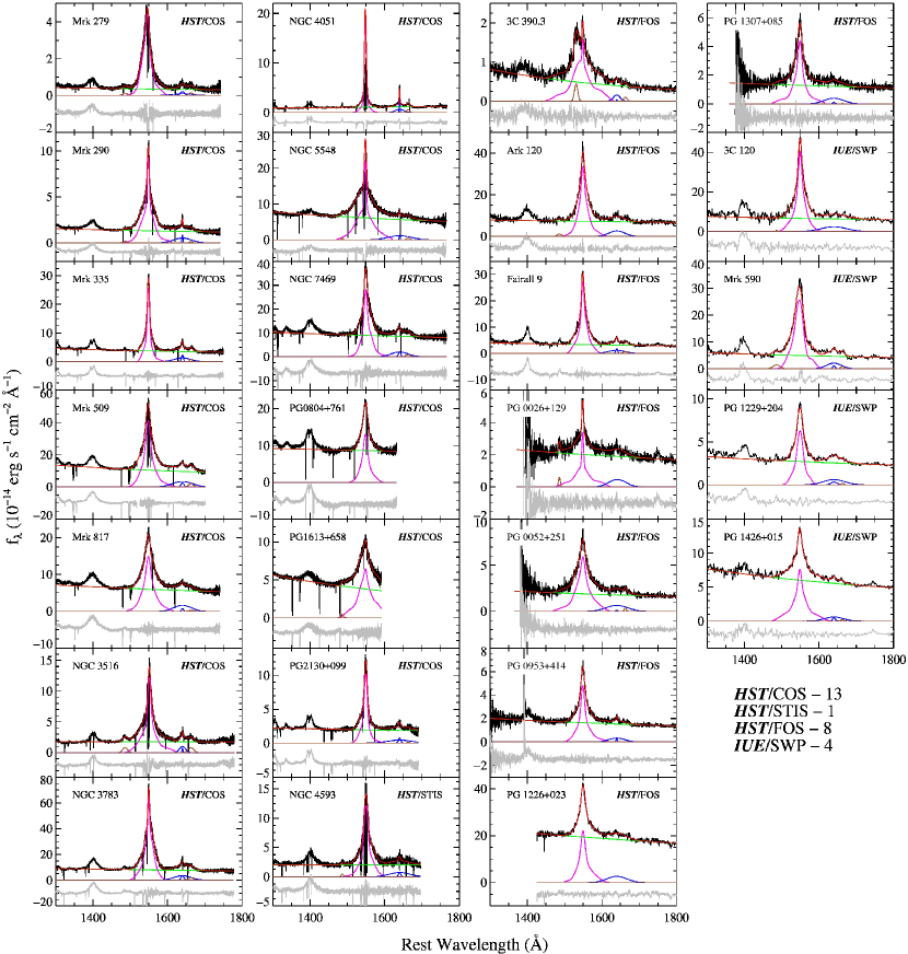
Figure 1.— Multi-component fitting results for the sample of 26 objects. In each panel, the observed UV spectrum (black) is overplotted with the best-fit model (red), which consists of a single power-law continuum (green), C IV $\lambda$1549Å emission line (magenta), He II $\lambda$1640Å emission line (blue), O III] $\lambda$1663Å emission line (brown), and N IV] $\lambda$1486Å emission line (brown). The residual (gray), differences between black and red lines, is presented at the bottom of each panel.

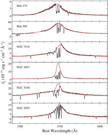
Figure 2.— The zoom-in view of the C IV for 6 objects, for which fitting results are uncertain due to the absorption at the line center. Black and red solid lines represent the observed spectra and the best-fit models, respectively.

In order to calibrate the C IV M_BH estimator, we measured the line width of C IV  and the continuum luminosity at 1350 Å, following the multi-component fitting procedure developed by Park et al. (2012b) with a modification for the C IV region. We first fitted a single power-law continuum using the typical emission-line-free windows in both sides of C IV  (i.e., $\sim 1340-1360$ Å or $\sim 1430-1470$ Å  and $\sim 1700-1730$ Å), which were slightly adjusted for each spectrum to avoid the contaminating absorption and emission features. We did not subtract the iron emission, since it is generally too weak to constrain at least in our data sets, although we indeed tested the pseudocontinuum model by including the UV Fe II template from Vestergaard & Wilkes (2001). After subtracting the best-fit power-law continuum, we simultaneously fitted the C IV complex region with the multi-component model consisting of a Gaussian function for the N IV] $\lambda$1486Å, a Gaussian function for the Si II $\lambda$1531Åwhenever clearly seen, a Gaussian function + a sixth-order Gauss-Hermite series for the C IV $\lambda$1549Å, two Gaussian functions for the He II $\lambda$1640Å, and a Gaussian function for the O III] $\lambda$1663Å. Note that we fitted the 1600 Å feature, which is contaminating the red wing of C IV, with a broad He II component (cf. Appendix A. in Fine et al. 2010; Marziani et al. 2010). In the fitting process, the centers of He II, O III], N IV], and Si II emission line components were fixed to be laboratory wavelengths. We suppressed some components in He II, O III], N IV], and Si II lines based on empirical tests with and without such components. Narrow absorption features were excluded automatically in the calculation of $\chi^{2}$ statistics by masking out the 3 sigma outliers below the smoothed spectrum (cf. Shen et al. 2011). Strong broad absorption features around the C IV line center were also masked out manually by setting exclusion windows from visual inspection.

Although it is still controversial whether or not to remove a narrow emission-line component from C IVbefore measuring the width, we use the full line profile of C IV, i.e., without subtracting a narrow emission-line component, in order to be consistent with other studies (VP06, Shen et al. 2011, Assef et al. 2011; Ho et al. 2012). We measured the continuum luminosities at $1350$ Å and $1450$ Å from the power-law model and measured the C IV line widths (FWHM and $\sigma$) from the best-fit model (i.e., a Gaussian function + a sixth-order Gauss-Hermite series) as shown in Figure 1. The measured line widths were corrected for the instrumental resolution following the standard practice by subtracting the instrumental resolution from the measured velocity in quadrature. In Figure 2, we explicitly show spectra and best-fit models for the objects showing absorption features at the center of C IV. Note that the fitting results are uncertain for these objects, in particular NGC 4051 (see Section 4.1).

To assess measurement uncertainties of the line width and continuum luminosity, we applied the Monte Carlo flux randomization method used by Park et al. (2012b; see also Shen et al. 2011). Using the $1,000$ realizations of resampled spectra made by randomly scattering flux values based on the flux errors, we fitted and measured the line width and continuum flux, and adopted the standard deviation of the distribution as the measurement uncertainties for individual objects as listed in Table 2.

3.1. Continuum Luminosities and Line Widths

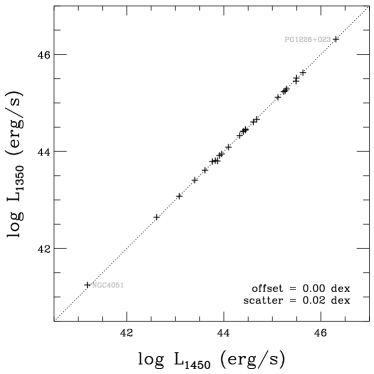
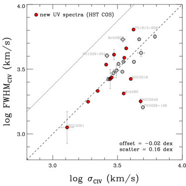
Figure 3.— Comparison of UV measurements. The top panel shows the consistency of luminosities measured at $1350$ Å and $1450$ Å, respectively. The bottom panel compares the C IV FWHM and line dispersion ($\sigma$), where both were measured from the full line profile. The ratio between FWHM and $\sigma$ is close to one (dashed line), indicating the line profile is more peaky than Gaussian (dotted line). Objects with new UV spectra from the HST COS is denoted with red filled circles. Average offset and 1$\sigma$ scatter are given in the lower right corner in each panel.

Figure 3 presents the continuum luminosities measured at $1350$ Å and $1450$ Å, respectively, which are commonly adopted for the C IV M_BH estimator. Since they are almost identical, we choose to use $L_{1350}$ for the mass estimator. The comparison between FWHM and $\sigma$ of C IV is plotted in the bottom panel of Figure 3. It shows on average, a one-to-one relation between FWHM and $\sigma$, indicating that the C IV profile is more peaky than a Gaussian profile, although there is large scatter.

3.2. Comparison to Previous Measurements

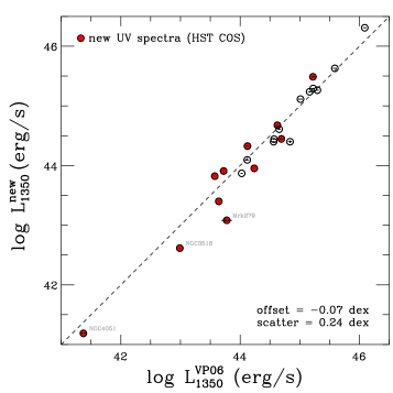
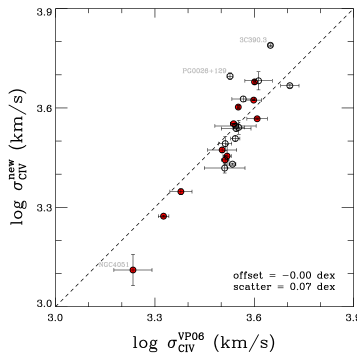
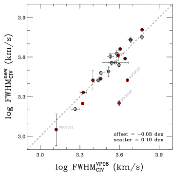
Figure 4.— Comparisons of the luminosity (top) and line width (middle and bottom) measured in this study and those by VP06. For VP06 values, the weighted average is plotted for given objects using the listed values in their Table 2. Average offset and 1$\sigma$ scatter are given in the lower right corner in each panel.

We compare our measurements with those in VP06 in Figure 4, using the common sample (23 out of 27 objects given in their Table 2, except for Mrk 79, Mrk 110, NGC 4151, and PG 1617+175). Since there are multiple measurements in VP06, we here show weighted average values of VP06 measurements for the purpose of comparison.

For the comparison of $L_{1350}$, there is 0.24 dex scatter, which may stem from a combination of the differences, e.g., adopted spectra and the Galactic extinction correction, between our study and VP06. We used the combined single spectra with the best quality while VP06 used all available SE spectra for each object. Especially for the objects with the new HST COS spectra (red filled circles) observed in different epochs, there could be an intrinsic difference due to the variability. In the case of the Galactic extinction correction, we utilized the recent values of $E(B-V)$ listed in the NED taken from the Schlafly & Finkbeiner (2011) recalibration, while VP06 used the original values from Schlegel et al. (1998).

When comparing our $\sigma_{\rm CIV}$ measurements to those of VP06, a slight positive systematic trend seems to be present (middle panel of Figure 4). The most likely origin of this trend is the difference in the adopted line width measurement methods between VP06 and this work. Based on the investigation by Fine et al. (2010), we modeled the C IV complex region with multiple components and measured line dispersion from the de-blended C IV line model profile, whereas VP06 measured line dispersion from the data without functional fits by limiting the C IV line profile range to $\pm 10,000$ km s^-1 of the line center, regardless of the intrinsic line width of each CIV profile. Thus, the line dispersion measured by VP06 will be biased if line wings are extended much further than the fixed line limit (i.e., underestimation) or the wings are smaller than the fixed line limit (i.e., overestimation by including other features). We avoid these biases by de-blending the C IV line from other lines using the multi-component fitting analysis and measuring the line widths from the best-fit models. Since the line dispersion is more sensitive to the line wings than the line core, the decomposition and thus recovery of the line wing profile from contaminating lines is essential.

The bottom panel of Figure 4 compares FWHM${}_{\rm C\ IV}$, indicating on average consistency between VP06 and this work, except for a few outliers. This is because FWHM is less sensitive to the line wings than $\sigma_{\rm C\ IV}$, hence the difference in the measuring method does not generate significant difference in measurements. Note that although FWHM is sensitive to the narrow-line component, both VP06 and our study used the full line profile without decomposing the broad and narrow components. Instead, another source of discrepancy comes from the fact that VP06 measured the line width directly from the data while in this study the best-fit models were used for line width measurements. Thus, there may be object-specific differences depending on how the absorptions above the ”half-maximum” flux level were dealt with by VP06, and how well the functional fits represent the peak of the profile in our study.

4. Updating the Calibration of the C IV SE $M_{\rm BH}$ estimator

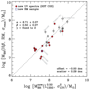
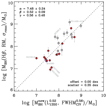
Figure 5.— Calibrations of $\sigma$-based SE BH masses (top) and FWHM-based SE BH masses (bottom) to the H$\beta$ RM-based BH masses. The new sample from the recent RM results is marked with a blue open square. The regressed parameters ($\alpha,\beta,\gamma$) with the uncertainty estimates are given in the upper left part in each panel.

By adopting H$\beta$ RM-based masses as true M_BH (see Table 1), we calibrate the C IV mass estimators by fitting

$$\log\left[\frac{M_{\rm BH}}{M_{\odot}}\right]~{}=~{}\alpha + \beta~{}\log\left(\frac{L_{1350}}{10^{44}~{}\rm erg~{}s^{-1}}\right)$$ (1)

$$~{}+~{} \gamma~{}\log\left[\frac{\varDelta V(\textrm{{C~{}IV}})}{1000~{}\rm km~{}s^{-1}}\right]~{},$$

where $L_{1350}$ is the monochromatic continuum luminosity at 1350 Å and $\varDelta V(\textrm{{C~{}IV}})$ is the line width of C IV, either FWHM_CIV or $\sigma_{\rm CIV}$. We regress Equation 1 to determine the free parameters ($\alpha,\beta,\gamma$) using the FITEXY estimator implemented in Park et al. (2012a). Note that this approach is different from that used by VP06, who adopted the luminosity slope from the size-luminosity relation and fixed the velocity slope to $2$. Instead, this method is consistent with the recent approaches described by Wang et al. (2009), Rafiee & Hall (2011b), and Shen & Liu (2012). Because a non-linear dependence is often observed between the line widths of H$\beta$ and C IV line (especially based on the FWHM; see Denney 2012 for a likely physical interpretation), leaving $\alpha$, $\beta$, and $\gamma$ as free parameters arguably results in a better statistical regression by accommodating the possible covariance between luminosity and line width.

4.1. New Calibrations

In Figure 5, we present the final best-fit calibration results for C IV-based mass estimators by directly comparing the C IV SE masses with the H$\beta$ RM-based masses, using Equation 1. The regression results with various conditions and the previous calibrations from the literature are listed in Table 3. We adopt the regression results without NGC 4051, which is subject to the largest measurement errors among our sample since modeling the C IV line of this object is highly uncertain due to the strong absorption at the center (see Fig. 2). In addition, the variability of NGC 4051 is expected to have a large amplitude since it is the lowest-luminosity object in our sample. Thus, NGC 4051 can add large scatter to the regression and potentially skew the slope because there is only a single object at the low-mass regime. Thus, excluding this object possibly will lead to less biased results in terms of sample selection and measurement uncertainties. We will present the results without NGC 4051 hereafter unless explicitly stated.

The slope of the velocity term, when it is treated as a free parameter, is closer to the virial assumption (i.e., 2) for the $\sigma_{\rm C\ IV}$-based estimator, i.e., $\gamma=1.74\pm 0.55$ ($\gamma=1.45\pm 0.53$ if NGC 4051 is included) than for the FWHM${}_{\rm C\ IV}$-based estimator, i.e., $\gamma=0.56\pm 0.48$ ($\gamma=0.52\pm 0.46$ if NGC 4051 is included). This reinforces the use of $\sigma$ for characterizing the line width of C IV, as suggested by Denney (2012, 2013; see also Peterson et al. 2004 and Park et al. 2012b for the case of H$\beta$). The slope of the luminosity term (i.e., $\beta=0.51\pm 0.08$ for $\sigma$; $\beta=0.52\pm 0.09$ for FWHM) is almost consistent to that of photoionization expectation (i.e., 0.5; Bentz et al. 2006) within the uncertainty. This may indicates that asynchronism between H$\beta$ and C IV measurements does not introduce a significant overall difference for our high-luminosity, high-quality calibration sample.

In this calibration, we treat $\beta$ and $\gamma$ as free parameters in addition to $\alpha$. Letting $\beta$ be a free parameter is required to reduce luminosity dependent systematics since we are dealing with non-contemporaneous H$\beta$ and C IV measurements, which is expected to be not necessarily linear. In addition, it is currently questionable to directly adopt the C IV size-luminosity relation (e.g., Kaspi et al. 2007) for the estimator since it is based on such a small sample. Relaxing the constraint of $\gamma=2$ for FWHM${}_{\rm C\ IV}$ can be corroborated by the investigation by Denney (2012), which shows that there are severe biases in measuring FWHM${}_{\rm C\ IV}$ due to the non-variable component and dependence on the line shape. These systematic uncertainties may be properly calibrated out by taking $\gamma$ as a free parameter. In the case of $\sigma_{\rm C\ IV}$, however, a similar systematic does not seem to be present for $\sigma_{\rm C\ IV}$ (see Denney 2012). Even if we allow $\gamma$ to be free, the regression slope for $\sigma_{\rm C\ IV}$ is consistent to the virial expectation (i.e., 2) within $1\sigma$ uncertainty, thus we opt to fixing $\gamma$ to a value of 2, avoiding systematic uncertainties due to small number statistics or sample-specific systematics. Thus, here we provide the best estimator for the C IV-based M_BH (see also, Fig. 5) as

$$\log\left[\frac{M_{\rm BH}}{M_{\odot}}\right] ~{}=~{} (6.71\pm 0.07)$$ (2)

$$~{}+~{} (0.50\pm 0.07)~{}\log\left(\frac{L_{1350}}{10^{44}~{}\rm erg~{}s^{-1}}\right)$$

$$~{}+~{} 2~{}\log\left[\frac{\sigma(\textrm{{C~{}IV}})}{1000~{}\rm km~{}s^{-1}}\right]$$

with the statistical scatter against RM masses of $0.29$ dex and

$$\log\left[\frac{M_{\rm BH}{\rm(SE)}}{M_{\odot}}\right] ~{}=~{} (7.48\pm 0.24)$$ (3)

$$~{}+~{} (0.52\pm 0.09)~{}\log\left(\frac{L_{1350}}{10^{44}~{}\rm erg~{}s^{-1}}\right)$$

$$~{}+~{} (0.56\pm 0.48)~{}\log\left[\frac{\rm FWHM(\textrm{{C~{}IV}})}{1000~{}\rm km~{}s^{-1}}\right]$$

with the statistical scatter against RM masses of $0.35$ dex. Apart from the interpretation of values of zero point and slopes, it is worth noting that these estimators are the best calibrated ones to reproduce H$\beta$ RM masses as closely as possible for the current sample and data sets.

4.2. Comparison to Previous Recipes

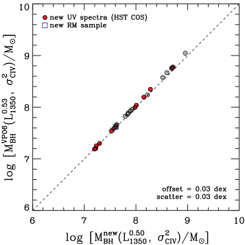
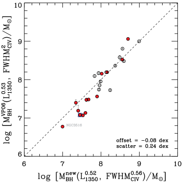
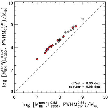
Figure 6.— Comparison of $\sigma$-based (top) and FWHM-based (middle) M_BH  respectively calculated using the estimators in this study and the estimators of VP06. In the bottom panel, M_BH calculated with the FWHM-based estimator from SL12 is compared to our mass estimates. Average offset and 1$\sigma$ scatter are given in the lower right corner in each panel.

In Figure 6, we present the systematic difference of M_BH estimates based on our new estimators (Equations 2 and 3) compared to the previous estimators from VP06 and SL12, respectively, using C IV line width and L₁₃₅₀ measurements. The $\sigma_{\rm C\ IV}$-based M_BH estimates show almost consistent results to VP06 with a slight offset of $\sim 0.03$, which is expected from a difference in the adopted values of the virial factor (i.e., $\log f=0.71$ here versus $\log f=0.74$ in VP06). In contrast, the comparison of FWHM${}_{\rm C\ IV}$-based masses, respectively estimated with our recipe and with that of VP06, shows large scatter and a systematic trend that the VP06 recipe underestimates M_BH in the low-mass regime and overestimates M_BH in the high-mass regime, compared to our recipe. The bottom panel of Figure 6 shows that the SL12 recipe systematically overestimates M_BH over the whole dynamic range of the sample (i.e., $\lesssim 10^{9}$ $M_{\odot}$). This is understandable because SL12 used the FWHM_Hβ-based M_BH in VP06 as a fiducial one and recalibrate the estimator using their high-mass ($>10^{9}$ $M_{\odot}$) QSOs. Thus, the calibration performed by SL12 in their limited dynamical range inherits the overestimation behavior of the VP06 recipe with respect to our recipe, and propagates it into the low mass regime with larger effect. In addition, SL12 subtracted a narrow C IV component before measuring FWHM of C IV, leading to an overestimated FWHM${}_{\rm C\ IV}$, compared to VP06 and our methods. We note that a large dynamic range is necessary for better calibration and investigation of the biases, as pointed out by SL12.

In order to explicitly compare the calibration methods used in here and VP06, we regress Equation 1 by fixing $\beta$ and/or $\gamma$ with the adopted values in VP06 as listed in Table 3. For the $\sigma$-based mass estimator, we obtain almost same calibration result ($\alpha=6.72\pm 0.06$) to that of VP06 ($\alpha=6.73\pm 0.01$) using the sample including NGC 4051. When NGC 4051 is exclude, the zero points reduces slightly ($\alpha=6.69\pm 0.06$) and intrinsic scatter becomes smaller. It is interesting to see the consistency of the $\sigma$-based calibration between our study and VP06, despite the systematic bias in $\sigma_{\rm CIV}$ measurements of VP06 as shown in Section 3.2. We interpret this as follows. Although there is a bias in the VP06 measurement method for $\sigma$, due to their choice of line limits (i.e., $\pm 10,000$ km s^-1), their $\sigma$-based M_BH measurements serendipitously scatter evenly below and above the central point of the mass scale of the sample, consequently resulting in a similar zero point regardless of the bias in $\sigma$ measurements. In the end the calibrations are very similar, however, the intrinsic scatter of our calibration is smaller than that of VP06, which demonstrates a general increase in accuracy of our $\sigma$-based masses over those of VP06, advocating for our $\sigma$ measurement prescription.

4.3. Difference in SMBH Population using the SDSS DR7 Quasar Catalog

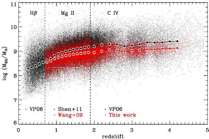
Figure 7.— Comparison of FWHM-based M_BH distributions as a function of redshift between the previous calibrations and the new ones in this study. FWHM${}_{\rm C\ IV}$ and L₁₃₅₀ for $\sim 100,000$ QSOs are taken from the SDSS DR7 quasar catalog (Shen et al. 2011) to calculate M_BH using different estimators. Black dots represent M_BH estimates using previous recipes of VP06 (H$\beta$; $z<0.7$), Shen+11 (Mg II; $0.7\leqslant z<1.9$), and VP06 (C IV; $z\geqslant 1.9$). Corresponding emission lines and M_BH recipes are indicated in upper and bottom parts with redshift separations marked with vertical dashed lines. For new M_BH estimates, red dots at $<1.9$ represent mass estimates using the calibration of Mg II by Wang et al. (2009), while red dots at $z\geqslant 1.9$ denote C IV-based M_BH estimates using our new recipe. Large filled circles indicate the median values in each redshift bin, with $\Delta z=0.1$ for $z\leqslant 1.9$ and $\Delta z=0.2$ for $z>1.9$. Average offset values of red filled circles from black filled circles are 0.17 dex for Mg II and 0.25 dex for C IV.

To demonstrate the effect of our new estimators on M_BH studies, we present in Figure 7 the M_BH distribution of the SDSS QSO sample as a function of redshift, based on various mass estimators. These masses are calculated using the FWHM${}_{\rm C\ IV}$ measurements from Shen et al. (2011), who provides only FWHM measurements using SDSS DR7 spectra. Note that FWHM${}_{\rm C\ IV}$-based M_BH determined with our new estimator is on average smaller by $\sim 0.25$ dex than that calculated with the previous estimator by VP06, since the VP06 recipe tends to overestimate M_BH in the high-mass regime as explained in Section 4.2. In contrast, there is a smooth transition between Mg II-based masses estimated from the recipe of Wang et al. (2009) and C IV-based masses from our new calibration since both estimators are based on the same calibration scheme (see Section 4).

Kelly & Shen (2013) derived a predicted maximum M_BH of broad-line QSOs as a function of redshift (their Figure 7), showing a slight trend that the maximum M_BH was larger at higher redshift. However, this subtle trend may simply be a result of systematic overestimation of C IV masses at high redshift because their mass determination was based on the VP06 recipe. Adopting our new C IV mass estimator may eliminate such a trend.

5. DISCUSSION AND CONCLUSIONS

We investigated the calibration of C IV M_BH estimators based on the updated sample of $26$ AGNs, for which both H$\beta$ reverberation masses and UV archival spectra were available. The sample of AGNs with RM masses as well as the UV spectra including C IV have been expanded and updated since the calibrations performed by VP06; it is therefore useful to revisit the calibration of the C IV-based mass estimators to provide the most consistent virial M_BH estimates using the C IV emission line. Major differences of the calibration method between VP06 and the current study is twofold. First, we derived line widths (i.e., line dispersion and FWHM) from the spectral fits by performing multi-component fitting on the C IV complex region to accurately de-blend C IV from other contaminating lines while VP06 measured the line width of CIV directly from the spectra. When “applying” a SE scaling relationship to calculate M_BH, it is important to use the same fitting and line width measurement prescriptions that were used in “calibrating” the scaling relationship because significant systematic differences can arise in M_BH estimates if different analysis and measurement techniques are utilized (e.g., Assef et al. 2011, Denney 2012, SL12, Park et al. 2012b). Second, we treated the slope parameters (i.e., $\beta$ and $\gamma$) in the virial M_BH equation (i.e., Eq. 1) as free parameters as in Wang et al. (2009), which is particularly important for FWHM.

We provided the best-fit calibrations for both $\sigma_{\rm C\ IV}$- and FWHM${}_{\rm C\ IV}$-based mass estimators. While we presented a consistent estimator for the $\sigma$-based masses to that of VP06, we obtained significantly different M_BH estimator for the FWHM-based masses, presumably due to relaxing the constraint of the virial expectation (i.e., $\gamma=2$) to mitigate the FWHM-dependent biases. We generally recommend to use the $\sigma$-based mass estimator if the $\sigma$ measurement is available, as it shows the better consistency with the virial relation, and $\sigma$-based masses show a smaller scatter than the FWHM-based masses when compared to H$\beta$ RM-based masses. Using $\sigma_{\rm C\ IV}$-based estimator is also preferred by Denney (2012), who showed that the $\sigma_{\rm C\ IV}$ measured from mean spectra is the better tracer of the broad-line velocity field than the FWHM${}_{\rm C\ IV}$ since FWHM of C IV is much more affected by the non-variable C IV core component.

Compared to the previously calibrated FWHM${}_{\rm C\ IV}$ estimator by VP06, our new estimator shows a systematic trend as a function of mass. The VP06 recipe overestimates M_BH in the high-mass regime (i.e., $\gtrsim 10^{8}M_{\odot}$) while it underestimate M_BH in the low-mass regime (i.e., $\lesssim 10^{8}M_{\odot}$), compared to C IV masses based on our new estimator. This systematic discrepancy is due to a combination of effects, including difference in the RM sample and updated RM masses, newly available UV spectra, emission-line fitting method, and calibration method. For the SDSS quasar sample (Shen et al. 2011), we find that M_BH estimates based on our new estimator are systematically smaller by $\sim 0.25$ dex than those based on the previous recipe of VP06.

One of the main differences in calibrating the FWHM${}_{\rm C\ IV}$-based mass estimator is that we fit the exponent of velocity ($\beta=0.56$) as in Eq. 3, instead of adopting $\beta=2$ as in VP06. This provides effectively the same effect as adopting a varying virial factor. If a constant virial factor is used for mass determination, then FWHM-based masses will show systematic difference compared to $\sigma$-based masses, since the FWHM/$\sigma$ ratio has a broad distribution, while the fiducial RM masses are derived with $\sigma$ measurements from rms spectra. To resolve this issue, Collin et al. (2006), for example, introduced varying virial factors for the FWHM_Hβ-based mass estimator depending on the range of the line widths. In our case, relaxing the virial (FWHM²) requirement in calibrating FWHM${}_{\rm C\ IV}$-based masses against $\sigma_{\rm H\beta}$-based RM masses provides virtually the same effect as adopting a varying virial factor, thus resulting in better consistency with $\sigma$-based masses. It also mitigates the bias caused by the contamination of the non-variable C IV emission component, where FWHM${}_{\rm C\ IV}$-based masses in objects with ’peaky’ (’boxy’) profiles are under- (over-) estimated with previous FWHM${}_{\rm C\ IV}$-based mass estimators.

The calibration of mass estimators provided in this study still suffers from a sample bias as in the case of VP06. The incompleteness or lack of low-mass objects (i.e., $\lesssim 10^{7}M_{\odot}$) in the current sample will be resolved when new HST STIS observations become available for six low-mass reverberation-mapped AGNs (GO-12922, PI: Woo). However, the extrapolation of this calibration to high-luminosity, higher-redshift AGNs more similar to the SDSS sample can only be realized with the extension of the RM sample to this regime — an endeavor that we strongly advocate.

Apart from the calibration analysis performed in this and previous studies, several schemes to correct for the C IV-based masses have been suggested in the literature to reduce the large scatter between the C IV-based masses and the H$\beta$-based masses. For example, Assef et al. (2011) suggested a prescription to reduce mass residuals using the ratio of the rest-frame UV to optical continuum luminosities based on a sample of 12 lensed quasars. Shen & Liu (2012) reported a poor correlation with large scatter between FWHM_Hβ and FWHM_CIV using a sample of 60 high-luminosity QSOs, showing that some part of the scatter correlated with the blueshift of C IV with respect to H$\beta$. They suggested a correction for the FWHM of C IV and C III] lines as a function of the C IV blueshift. Recently, Denney (2012) showed that the C IV line profile consists of both non-variable and variable components based on the sample of seven AGNs with C IV reverberation data, and concluded that this non-variable component is a main source of the large scatter of the C IV SE M_BH. They provided an empirical correction for the FWHM-based mass depending on the line shape as parameterized as the ratio of FWHM to the line dispersion. Since the C IV line region is more likely to be affected by non-virial motions such as outflows and winds than the lower ionization line region, such as H$\beta$ (e.g., Shen et al. 2008; Richards et al. 2011), aforementioned corrections are also important and worth investigating further with a larger sample with enlarged dynamic range.

In general, correcting for possible systematic biases and providing accurate M_BH estimates is crucial for studies of the cosmic evolution of BH population, particularly at high-redshifts (e.g., Fine et al. 2006; Shen et al. 2008, 2011, Shen & Kelly 2012; Kelly & Shen 2013). Thus, it is important to ensure a reliable calibration at the high-mass end ($\gtrsim 10^{9}$ $M_{\odot}$) since the C IV mass estimators are most applicable to high-mass AGNs at high-redshift utilizing optical spectroscopic data from large AGN surveys. Note that the current RM sample used for calibrating C IV mass estimators still suffers from the lack of high-luminosity AGNs, suggesting that the RM sample may not best represent the high-luminosity QSOs at high-redshifts, i.e., SDSS QSOs. Thus, obtaining direct C IV reverberation mapping results for high-mass QSOs will be even more useful (see Kaspi et al. 2007 for tentative results), despite the practical observational challenges. Such measurements will be used to better determine a reliable C IV size-luminosity relation and to directly investigate non-varying component of C IV.

Table 1Optical spectral properties from H$\beta$ reverberation mapping

Object	$z$	$\tau_{\rm cent}$	$\sigma_{\rm rms}$	FWHMrms	$\log(M_{\rm BH}$/$M_{\odot}$)	References
		(H$\beta$)	(H$\beta$)	(H$\beta$)	(RM)
		(days)	(km s-1)	(km s-1)
(1)	(2)	(3)	(4)	(5)	(6)	(7)
3C120	$0.03301$	$27.2^{+1.1}_{-1.1}$	$1514\pm 65$	$2539\pm 466$	$7.80\pm 0.04$	6
3C390.3	$0.05610$	$23.60^{+6.45}_{-6.45}$	$3105\pm 81$	$9958\pm 1046$	$8.43\pm 0.10$	1
Ark120	$0.03230$	$39.05^{+4.57}_{-4.57}$	$1896\pm 44$	$5364\pm 168$	$8.14\pm 0.06$	1
Fairall9	$0.04702$	$17.40^{+3.75}_{-3.75}$	$3787\pm 197$	$6901\pm 707$	$8.38\pm 0.10$	1
Mrk279	$0.03045$	$16.70^{+3.90}_{-3.90}$	$1420\pm 96$	$3385\pm 349$	$7.51\pm 0.12$	1
Mrk290	$0.02958$	$8.72^{+1.21}_{-1.02}$	$1609\pm 47$	$4270\pm 157$	$7.36\pm 0.07$	4
Mrk335	$0.02578$	$14.1^{+0.4}_{-0.4}$	$1293\pm 64$	$1025\pm 35$	$7.37\pm 0.05$	6
Mrk509	$0.03440$	$79.60^{+5.75}_{-5.75}$	$1276\pm 28$	$2715\pm 101$	$8.12\pm 0.04$	1
Mrk590	$0.02638$	$24.23^{+2.11}_{-2.11}$	$1653\pm 40$	$2512\pm 101$	$7.65\pm 0.07$	1
Mrk817	$0.03145$	$19.05^{+2.45}_{-2.45}$	$1636\pm 57$	$3992\pm 302$	$7.66\pm 0.07$	1
NGC3516	$0.00884$	$11.68^{+1.02}_{-1.53}$	$1591\pm 10$	$5175\pm 96$	$7.47\pm 0.05$	4
NGC3783	$0.00973$	$10.20^{+2.80}_{-2.80}$	$1753\pm 141$	$3093\pm 529$	$7.44\pm 0.08$	1
NGC4051	$0.00234$	$1.87^{+0.54}_{-0.50}$	$927\pm 64$	$1034\pm 41$	$6.20\pm 0.14$	4
NGC4593	$0.00900$	$3.73^{+0.75}_{-0.75}$	$1561\pm 55$	$4141\pm 416$	$6.96\pm 0.09$	2
NGC5548	$0.01717$	$4.18^{+0.86}_{-1.30}$	$3900\pm 266$	$12539\pm 1927$	$7.80\pm 0.14$	3, 5
NGC7469	$0.01632$	$4.50^{+0.75}_{-0.75}$	$1456\pm 207$	$2169\pm 459$	$7.05\pm 0.05$	1
PG0026+129	$0.14200$	$111.00^{+26.20}_{-26.20}$	$1773\pm 285$	$1719\pm 495$	$8.56\pm 0.11$	1
PG0052+251	$0.15500$	$89.80^{+24.30}_{-24.30}$	$1783\pm 86$	$4165\pm 381$	$8.54\pm 0.09$	1
PG0804+761	$0.10000$	$146.90^{+18.85}_{-18.85}$	$1971\pm 105$	$2012\pm 845$	$8.81\pm 0.05$	1
PG0953+414	$0.23410$	$150.10^{+22.10}_{-22.10}$	$1306\pm 144$	$3002\pm 398$	$8.41\pm 0.09$	1
PG1226+023	$0.15830$	$306.80^{+79.70}_{-79.70}$	$1777\pm 150$	$2598\pm 299$	$8.92\pm 0.09$	1
PG1229+204	$0.06301$	$37.80^{+21.45}_{-21.45}$	$1385\pm 111$	$3415\pm 320$	$7.83\pm 0.23$	1
PG1307+085	$0.15500$	$105.60^{+41.30}_{-41.30}$	$1820\pm 122$	$5058\pm 524$	$8.61\pm 0.12$	1
PG1426+015	$0.08647$	$95.00^{+33.50}_{-33.50}$	$3442\pm 308$	$6323\pm 1295$	$9.08\pm 0.13$	1
PG1613+658	$0.12900$	$40.10^{+15.10}_{-15.10}$	$2547\pm 342$	$7897\pm 1792$	$8.42\pm 0.22$	1
PG2130+099	$0.06298$	$12.8^{+1.2}_{-0.9}$	$1825\pm 65$	$2097\pm 102$	$7.63\pm 0.04$	6

Note. — Col. (1) Name. Col. (2) Redshifts are from the NASA/IPAC Extragalactic Database (NED). Col. (3) Rest-frame H$\beta$ time lag measurements. Col. (4) Line dispersion ($\sigma_{\rm line}$) measured from rms spectra. Col. (5) FWHM measured from rms spectra Col. (6) M_BH estimates from reverberation mapping: $M_{\rm BH}({\rm RM})=fc\tau_{\rm cent}\sigma_{\rm rms}^{2}/G$ where the virial factor $f$ is adopted from Park et al. (2012a) (i.e., $\log f=0.71$). Col. (7) References. 1. Peterson et al. 2004; 2. Denney et al. 2006; 3. Bentz et al. 2009; 4. Denney et al. 2010; 5. Park et al. 2012b; 6. Grier et al. 2012.

Table 2Ultraviolet spectral properties from C IV single-epoch estimates

Object	Telescope/Instrument	Date Observed	S/N	$E(B-V)$	$\log(\lambda L_{\lambda}/$erg s-1$)$	$\sigma_{\rm SE}$	FWHMSE	$\log(M_{\rm BH}$/$M_{\odot}$)	$\log(M_{\rm BH}$/$M_{\odot}$)	Notes
			(1450Å or 1700Å)		(1350Å)	(C IV)	(C IV)	($\sigma$(C IV), SE)	(FWHM(C IV), SE)
			(pix-1)	(mag)		(km s-1)	(km s-1)
(1)	(2)	(3)	(4)	(5)	(6)	(7)	(8)	(9)	(10)	(11)
3C120	IUE/SWP	1994-02-19,27;1994-03-11	$12$	0.263	$44.399\pm 0.021$	$3106\pm 157$	$3093\pm 291$	$7.89\pm 0.05$	$7.96\pm 0.03$	$\cdots$
3C390.3	HST/FOS	1996-03-31	$18$	0.063	$43.869\pm 0.003$	$6154\pm 65$	$5645\pm 202$	$8.22\pm 0.01$	$7.83\pm 0.01$	$\cdots$
Ark120	HST/FOS	1995-07-29	$17$	0.114	$44.400\pm 0.005$	$3219\pm 53$	$3471\pm 108$	$7.93\pm 0.01$	$7.99\pm 0.01$	$\cdots$
Fairall9	HST/FOS	1993-01-22	$24$	0.023	$44.442\pm 0.004$	$2694\pm 20$	$2649\pm 77$	$7.79\pm 0.01$	$7.95\pm 0.01$	$\cdots$
Mrk279	HST/COS	2011-06-27	$9$	0.014	$43.082\pm 0.004$	$2973\pm 53$	$4093\pm 388$	$7.20\pm 0.02$	$7.35\pm 0.02$	$\cdots$
Mrk290	HST/COS	2009-10-28	$24$	0.014	$43.611\pm 0.002$	$3531\pm 32$	$2052\pm 36$	$7.61\pm 0.01$	$7.45\pm 0.01$	$\cdots$
Mrk335	HST/COS	2009-10-31;2010-02-08	$29$	0.032	$43.953\pm 0.001$	$1876\pm 12$	$1772\pm 14$	$7.23\pm 0.01$	$7.59\pm 0.01$	$\cdots$
Mrk509	HST/COS	2009-12-10,11	$107$	0.051	$44.675\pm 0.001$	$3568\pm 9$	$3872\pm 18$	$8.15\pm 0.01$	$8.16\pm 0.01$	$\cdots$
Mrk590	IUE/SWP	1991-01-14	$17$	0.033	$44.094\pm 0.007$	$3479\pm 165$	$5362\pm 266$	$7.84\pm 0.04$	$7.94\pm 0.01$	$\cdots$
Mrk817	HST/COS	2009-08-04;2009-12-28	$38$	0.006	$44.326\pm 0.001$	$3692\pm 23$	$4580\pm 48$	$8.01\pm 0.01$	$8.02\pm 0.01$	$\cdots$
NGC3516	HST/COS	2010-10-04;2011-01-22	$20$	0.038	$42.615\pm 0.002$	$4006\pm 49$	$2658\pm 34$	$7.22\pm 0.01$	$7.00\pm 0.01$	abs
NGC3783	HST/COS	2011-05-26	$29$	0.105	$43.400\pm 0.001$	$2774\pm 91$	$2656\pm 444$	$7.30\pm 0.03$	$7.41\pm 0.04$	$\cdots$
NGC4051	HST/COS	2009-12-11	$23$	0.011	$41.187\pm 0.001$	$1290\pm 139$	$1122\pm 309$	$5.53\pm 0.09$	$6.05\pm 0.07$	abs
NGC4593	HST/STIS	2002-06-23,24	$10$	0.022	$43.761\pm 0.005$	$2946\pm 162$	$2952\pm 166$	$7.53\pm 0.05$	$7.62\pm 0.01$	$\cdots$
NGC5548	HST/COS	2011-06-16,17	$36$	0.018	$43.822\pm 0.001$	$4772\pm 80$	$1785\pm 82$	$7.98\pm 0.01$	$7.53\pm 0.01$	abs
NGC7469	HST/COS	2010-10-16	$32$	0.061	$43.909\pm 0.001$	$2849\pm 237$	$2725\pm 66$	$7.57\pm 0.07$	$7.68\pm 0.01$	$\cdots$
PG0026+129	HST/FOS	1994-11-27	$25$	0.063	$45.236\pm 0.005$	$4965\pm 113$	$1604\pm 50$	$8.72\pm 0.02$	$8.24\pm 0.01$	$\cdots$
PG0052+251	HST/FOS	1993-07-22	$21$	0.042	$45.292\pm 0.004$	$4648\pm 50$	$5380\pm 87$	$8.69\pm 0.01$	$8.56\pm 0.01$	$\cdots$
PG0804+761	HST/COS	2010-06-12	$34$	0.031	$45.493\pm 0.001$	$2585\pm 20$	$3429\pm 23$	$8.28\pm 0.01$	$8.56\pm 0.01$	$\cdots$
PG0953+414	HST/FOS	1991-06-18	$18$	0.012	$45.629\pm 0.005$	$3448\pm 55$	$3021\pm 74$	$8.60\pm 0.01$	$8.60\pm 0.01$	$\cdots$
PG1226+023	HST/FOS	1991-01-14,15	$93$	0.018	$46.309\pm 0.001$	$3513\pm 29$	$3609\pm 29$	$8.96\pm 0.01$	$8.99\pm 0.01$	$\cdots$
PG1229+204	IUE/SWP	1982-05-01,02	$28$	0.024	$44.609\pm 0.009$	$2621\pm 90$	$4023\pm 163$	$7.85\pm 0.03$	$8.14\pm 0.01$	$\cdots$
PG1307+085	HST/FOS	1993-07-21	$14$	0.030	$45.113\pm 0.006$	$4237\pm 80$	$3604\pm 111$	$8.52\pm 0.02$	$8.37\pm 0.01$	$\cdots$
PG1426+015	IUE/SWP	1985-03-01,02	$45$	0.028	$45.263\pm 0.004$	$4808\pm 305$	$4220\pm 258$	$8.71\pm 0.06$	$8.49\pm 0.02$	$\cdots$
PG1613+658	HST/COS	2010-04-08,09,10	$37$	0.023	$45.488\pm 0.001$	$4204\pm 17$	$6398\pm 51$	$8.70\pm 0.01$	$8.71\pm 0.01$	$\cdots$
PG2130+099	HST/COS	2010-10-28	$22$	0.039	$44.447\pm 0.001$	$2225\pm 47$	$2147\pm 18$	$7.63\pm 0.02$	$7.90\pm 0.01$	$\cdots$

Note. — Col. (1) Name. Col. (2) Telescope/Instrument from which archival UV spectra were obtained. Note that the new COS spectra were obtained after 2009. Col. (3) Observation date for combined spectra. Col. (4) Signal-to-noise ratio per pixel at 1450Å or 1700Å in rest-frame. Col. (5) $E(B-V)$ are from the NASA/IPAC Extragalactic Database (NED) based on the recalibration of Schlafly & Finkbeiner (2011). Col. (6) Continuum luminosity measured at 1350Å. Col. (7) Line dispersion ($\sigma_{\rm line}$) measured from SE spectra. Col. (8) FWHM measured from SE spectra. Col. (9) SE mass estimates based on $\sigma_{\rm line}$ from the new estimator. Col. (10) SE mass estimates based on FWHM from the new estimator. Col. (11) abs: The C IV line profile is affected by a strong absorption near the line center. Thus the emission-line modeling could be uncertain although that region was masked out.

Table 3C IV Mass Calibration results
$\log[M_{\rm BH}{\rm(RM)}/M_{\odot}]=~{}\alpha~{}+~{}\beta~{}\log(L_{1350}/10^{44}~{}\rm erg~{}s^{-1})~{}+~{}\gamma~{}\log[\varDelta V(\textrm{{C~{}IV}})/1000~{}\rm km~{}s^{-1}]$

$\varDelta V(\textrm{{C~{}IV}})$	$\alpha$	$\beta$	$\gamma$	$\sigma_{{\mathop{\rm int}}}$	mean offset	1$\sigma$ scatter	Ref.
					(dex)	(dex)
Previous calibrations
$\sigma_{\rm line}$	$6.73\pm 0.01$	$0.53$	$2$	$0.33$	$\cdots$	$\cdots$	VP06
$\sigma_{\rm line}$	$6.73\pm 0.02$	$0.53$	$2$	$0.37$	$\cdots$	$\cdots$	VP06
FWHM	$6.66\pm 0.01$	$0.53$	$2$	$0.36$	$\cdots$	$\cdots$	VP06
FWHM	$6.69\pm 0.01$	$0.53$	$2$	$0.43$	$\cdots$	$\cdots$	VP06
FWHM	$8.021$	$0.471$	$0.242$	$\cdots$	$0.03$	$0.28$	SL12
This work
$\sigma_{\rm line}$	$7.02\pm 0.29$	$0.46\pm 0.07$	$1.45\pm 0.53$	$0.30\pm 0.04$	$0.00$	$0.298$
FWHM	$7.51\pm 0.21$	$0.51\pm 0.08$	$0.52\pm 0.46$	$0.34\pm 0.05$	$0.00$	$0.340$
This work (fixing $\gamma=2$)
$\sigma_{\rm line}$	$6.75\pm 0.07$	$0.43\pm 0.07$	$2$	$0.30\pm 0.05$	$0.00$	$0.308$
FWHM	$6.81\pm 0.09$	$0.40\pm 0.08$	$2$	$0.41\pm 0.05$	$0.00$	$0.421$
This work (fixing $\beta=0.5$)
$\sigma_{\rm line}$	$7.07\pm 0.27$	$0.5$	$1.34\pm 0.48$	$0.29\pm 0.04$	$0.00$	$0.301$
FWHM	$7.50\pm 0.18$	$0.5$	$0.54\pm 0.36$	$0.33\pm 0.04$	$0.00$	$0.340$
This work (fixing $\beta=0.5$ and $\gamma=2$)
$\sigma_{\rm line}$	$6.73\pm 0.06$	$0.5$	$2$	$0.30\pm 0.04$	$0.00$	$0.318$
FWHM	$6.78\pm 0.08$	$0.5$	$2$	$0.41\pm 0.05$	$0.00$	$0.439$
This work (fixing $\beta=0.53$ and $\gamma=2$ for the comparison to VP06)
$\sigma_{\rm line}$	$6.72\pm 0.06$	$0.53$	$2$	$0.31\pm 0.04$	$0.00$	$0.328$
FWHM	$6.77\pm 0.08$	$0.53$	$2$	$0.42\pm 0.05$	$0.00$	$0.449$
This work (w/o NGC 4051)
$\sigma_{\rm line}$	$6.84\pm 0.30$	$0.51\pm 0.08$	$1.74\pm 0.55$	$0.29\pm 0.04$	$0.00$	$0.293$
FWHM	$\bf 7.48\pm 0.24$	$\bf 0.52\pm 0.09$	$\bf 0.56\pm 0.48$	$0.35\pm 0.05$	$0.00$	$0.347$	best-fit
This work (w/o NGC 4051; fixing $\gamma=2$)
$\sigma_{\rm line}$	$\bf 6.71\pm 0.07$	$\bf 0.50\pm 0.07$	$\bf 2$	$0.28\pm 0.04$	$0.00$	$0.295$	best-fit
FWHM	$6.78\pm 0.10$	$0.45\pm 0.10$	$2$	$0.41\pm 0.05$	$0.00$	$0.419$
This work (w/o NGC 4051; fixing $\beta=0.5$)
$\sigma_{\rm line}$	$6.84\pm 0.29$	$0.5$	$1.75\pm 0.51$	$0.28\pm 0.04$	$0.00$	$0.293$
FWHM	$7.47\pm 0.23$	$0.5$	$0.59\pm 0.44$	$0.34\pm 0.04$	$0.00$	$0.347$
This work (w/o NGC 4051; fixing $\beta=0.5$ and $\gamma=2$)
$\sigma_{\rm line}$	$6.71\pm 0.06$	$0.5$	$2$	$0.28\pm 0.04$	$0.00$	$0.295$
FWHM	$6.75\pm 0.08$	$0.5$	$2$	$0.40\pm 0.05$	$0.00$	$0.422$
This work (w/o NGC 4051; fixing $\beta=0.53$ and $\gamma=2$ for the comparison to VP06)
$\sigma_{\rm line}$	$6.69\pm 0.06$	$0.53$	$2$	$0.28\pm 0.04$	$0.00$	$0.296$
FWHM	$6.74\pm 0.08$	$0.53$	$2$	$0.41\pm 0.05$	$0.00$	$0.425$

Note. — The mean offset and $1\sigma$ scatter for our calibrations are measured from the average and standard deviation of mass residuals between RM masses and calibrated SE masses, $\varDelta=\log M_{\rm BH}{\rm(RM)}-\log M_{\rm BH}{\rm(SE)}$.

References

- Assef et al. (2011) Assef, R. J., Denney, K. D., Kochanek, C. S., et al. 2011, ApJ, 742, 93
- Barth et al. (2011a) Barth, A. J., Nguyen, M. L., Malkan, M. A., et al. 2011a, ApJ, 732, 121
- Barth et al. (2011b) Barth, A. J., Pancoast, A., Thorman, S. J., et al. 2011b, ApJ, 743, L4
- Baskin & Laor (2005) Baskin, A., & Laor, A. 2005, MNRAS, 356, 1029
- Bennert et al. (2010) Bennert, V. N., Treu, T., Woo, J.-H., et al. 2010, ApJ, 708, 1507
- Bennert et al. (2011) Bennert, V. N., Auger, M. W., Treu, T., Woo, J.-H., & Malkan, M. A. 2011, ApJ, 742, 107
- Bentz et al. (2006) Bentz, M. C., Peterson, B. M., Pogge, R. W., Vestergaard, M., & Onken, C. A. 2006, ApJ, 644, 133
- Bentz et al. (2009) Bentz, M. C., Peterson, B. M., Netzer, H., Pogge, R. W., & Vestergaard, M. 2009, ApJ, 697, 160
- Bentz et al. (2013) Bentz, M. C., Denney, K. D., Grier, C. J., et al. 2013, ApJ, in press, (arXiv:1303.1742)
- Canalizo et al. (2012) Canalizo, G., Wold, M., Hiner, K. D., et al. 2012, ApJ, 760, 38
- Collin et al. (2006) Collin, S., Kawaguchi, T., Peterson, B. M., & Vestergaard, M. 2006, A&A, 456, 75
- Denney et al. (2006) Denney, K. D., Bentz, M. C., Peterson, B. M., et al. 2006, ApJ, 653, 152
- Denney et al. (2009) Denney, K. D., Peterson, B. M., Dietrich, M., Vestergaard, M., & Bentz, M. C. 2009, ApJ, 692, 246
- Denney et al. (2010) Denney, K. D., Peterson, B. M., Pogge, R. W., et al. 2010, ApJ, 721, 715
- Denney (2012) Denney, K. D. 2012, ApJ, 759, 44
- Denney et al. (2013) Denney, K. D., Pogge, R. W., Assef, R. J., et al. 2013, ApJ, submitted, (arXiv:1303.3889)
- Dietrich et al. (2009) Dietrich, M., Mathur, S., Grupe, D., & Komossa, S. 2009, ApJ, 696, 1998
- Ferrarese & Merritt (2000) Ferrarese, L., & Merritt, D. 2000, ApJ, 539, L9
- Fine et al. (2006) Fine, S., Croom, S. M., Miller, L., et al. 2006, MNRAS, 373, 613
- Fine et al. (2010) Fine, S., Croom, S. M., Bland-Hawthorn, J., et al. 2010, MNRAS, 409, 591
- Fitzpatrick (1999) Fitzpatrick, E. L. 1999, PASP, 111, 63
- Gebhardt et al. (2000) Gebhardt, K., Bender, R., Bower, G., et al. 2000, ApJ, 539, L13
- Graham et al. (2011) Graham, A. W., Onken, C. A., Athanassoula, E., & Combes, F. 2011, MNRAS, 412, 2211
- Greene et al. (2010) Greene, J. E., Peng, C. Y., & Ludwig, R. R. 2010, ApJ, 709, 937
- Grier et al. (2012) Grier, C. J., Peterson, B. M., Pogge, R. W., et al. 2012, ApJ, 755, 60
- Hiner et al. (2012) Hiner, K. D., Canalizo, G., Wold, M., Brotherton, M. S., & Cales, S. L. 2012, ApJ, 756, 162
- Ho et al. (2012) Ho, L. C., Goldoni, P., Dong, X.-B., Greene, J. E., & Ponti, G. 2012, ApJ, 754, 11
- Kaspi et al. (2000) Kaspi, S., Smith, P. S., Netzer, H., et al. 2000, ApJ, 533, 631
- Kaspi et al. (2005) Kaspi, S., Maoz, D., Netzer, H., et al. 2005, ApJ, 629, 61
- Kaspi et al. (2007) Kaspi, S., Brandt, W. N., Maoz, D., et al. 2007, ApJ, 659, 997
- Keeney et al. (2012) Keeney, B. A., Danforth, C. W., Stocke, J. T., France, K., & Green, J. C. 2012, PASP, 124, 830
- Kelly & Bechtold (2007) Kelly, B. C., & Bechtold, J. 2007, ApJS, 168, 1
- Kelly & Shen (2013) Kelly, B. C., & Shen, Y. 2013, ApJ, 764, 45
- Leighly & Moore (2004) Leighly, K. M., & Moore, J. R. 2004, ApJ, 611, 107
- Magorrian et al. (1998) Magorrian, J., Tremaine, S., Richstone, D., et al. 1998, AJ, 115, 2285
- Marziani et al. (2010) Marziani, P., Sulentic, J. W., Negrete, C. A., et al. 2010, MNRAS, 409, 1033
- McGill et al. (2008) McGill, K. L., Woo, J.-H., Treu, T., & Malkan, M. A. 2008, ApJ, 673, 703
- McLure & Dunlop (2004) McLure, R. J., & Dunlop, J. S. 2004, MNRAS, 352, 1390
- McLure & Jarvis (2002) McLure, R. J., & Jarvis, M. J. 2002, MNRAS, 337, 109
- Merloni et al. (2010) Merloni, A., Bongiorno, A., Bolzonella, M., et al. 2010, ApJ, 708, 137
- Metzroth et al. (2006) Metzroth, K. G., Onken, C. A., & Peterson, B. M. 2006, ApJ, 647, 901
- Netzer et al. (2007) Netzer, H., Lira, P., Trakhtenbrot, B., Shemmer, O., & Cury, I. 2007, ApJ, 671, 1256
- Onken et al. (2004) Onken, C. A., Ferrarese, L., Merritt, D., et al. 2004, ApJ, 615, 645
- Park et al. (2012a) Park, D., Kelly, B. C., Woo, J.-H., & Treu, T. 2012a, ApJS, 203, 6
- Park et al. (2012b) Park, D., Woo, J.-H., Treu, T., et al. 2012b, ApJ, 747, 30
- Peng et al. (2006) Peng, C. Y., Impey, C. D., Rix, H.-W., et al. 2006, ApJ, 649, 616
- Peterson (1993) Peterson, B. M. 1993, PASP, 105, 247
- Peterson et al. (2004) Peterson, B. M., Ferrarese, L., Gilbert, K. M., et al. 2004, ApJ, 613, 682
- Peterson et al. (2005) Peterson, B. M., Bentz, M. C., Desroches, L.-B., et al. 2005, ApJ, 632, 799
- Rafiee & Hall (2011) Rafiee, A., & Hall, P. B. 2011a, ApJS, 194, 42
- Rafiee & Hall (2011) Rafiee, A., & Hall, P. B. 2011b, MNRAS, 415, 2932
- Richards et al. (2011) Richards, G. T., Kruczek, N. E., Gallagher, S. C., et al. 2011, AJ, 141, 167
- Salviander et al. (2007) Salviander, S., Shields, G. A., Gebhardt, K., & Bonning, E. W. 2007, ApJ, 662, 131
- Schlafly & Finkbeiner (2011) Schlafly, E. F., & Finkbeiner, D. P. 2011, ApJ, 737, 103
- Schlegel et al. (1998) Schlegel, D. J., Finkbeiner, D. P., & Davis, M. 1998, ApJ, 500, 525
- Shen et al. (2008) Shen, Y., Greene, J. E., Strauss, M. A., Richards, G. T., & Schneider, D. P. 2008, ApJ, 680, 169
- Shen et al. (2011) Shen, Y., Richards, G. T., Strauss, M. A., et al. 2011, ApJS, 194, 45
- Shen & Liu (2012) Shen, Y., & Liu, X. 2012, ApJ, 753, 125
- Shen & Kelly (2012) Shen, Y., & Kelly, B. C. 2012, ApJ, 746, 169
- Sulentic et al. (2007) Sulentic, J. W., Bachev, R., Marziani, P., Negrete, C. A., & Dultzin, D. 2007, ApJ, 666, 757
- Trakhtenbrot & Netzer (2012) Trakhtenbrot, B., & Netzer, H. 2012, MNRAS, 427, 3081
- Treu et al. (2007) Treu, T., Woo, J.-H., Malkan, M. A., & Blandford, R. D. 2007, ApJ, 667, 117
- Vestergaard (2002) Vestergaard, M. 2002, ApJ, 571, 733
- Vestergaard & Peterson (2006) Vestergaard, M., & Peterson, B. M. 2006, ApJ, 641, 689
- Vestergaard & Wilkes (2001) Vestergaard, M., & Wilkes, B. J. 2001, ApJS, 134, 1
- Wandel et al. (1999) Wandel, A., Peterson, B. M., & Malkan, M. A. 1999, ApJ, 526, 579
- Wang et al. (2009) Wang, J.-G., Dong, X.-B., Wang, T.-G., et al. 2009, ApJ, 707, 1334
- Woo et al. (2006) Woo, J.-H., Treu, T., Malkan, M. A., & Blandford, R. D. 2006, ApJ, 645, 900
- Woo et al. (2008) Woo, J.-H., Treu, T., Malkan, M. A., & Blandford, R. D. 2008, ApJ, 681, 925
- Woo et al. (2010) Woo, J.-H., Treu, T., Barth, A. J., et al. 2010, ApJ, 716, 269
- Woo et al. (2013) Woo, J.-H., Schulze, A., Park, D., Kang, W.-R., Kim, S. C., & Riechers, D. 2013, ApJ, submitted